


1. Introduction
The wall-pressure fluctuations induced by a turbulent boundary layer (TBL) constitute an important source of noise and vibration in many applications. Such fluctuations, caused by eddies correlated over limited regions in the boundary layer, result in flow-induced loads that can either radiate noise directly or excite the underlying structure generating vibration and noise, mainly in the low to mid audio frequency range, where human annoyance to noise is particularly important. This topic is also of interest for many engineering problems. A few examples among many are fatigue cracking on panels of an aircraft fuselage induced by high-speed turbulent flow, or cabin noise transmitted by flexible structures loaded by TBLs excitation. In marine transportation, the noise generated by wall-pressure fluctuations has become quite important when considering the need for improved inboard comfort in high-speed ships. In particular, acoustic waves created by the scattering of the wall-pressure fluctuations at a sharp-edged body, such as a wing or a fan blade, are the cause of broadband noise, also known as trailing-edge (TE) noise (Tam & Yu Reference Tam and Yu1975; Brooks & Hodgson Reference Brooks and Hodgson1981; Lee et al. Reference Lee, Ayton, Bertagnolio, Moreau, Chong and Joseph2021). As indicated in most aerofoil TE noise models based on acoustic analogies (Curle Reference Curle1955; Ffowcs-Williams & Hall Reference Ffowcs-Williams and Hall1970; Howe Reference Howe1978), the wall-pressure fluctuations can be an efficient sound source of dipole type that can be dominant at low Mach numbers. Indeed, such a noise mechanism is responsible for part or most of the airframe, propeller, low- and high-speed rotor and wind turbine noise, as well as other noise problems.
In order to predict the disturbance produced by such turbulent flows, it is first necessary to model all the fluctuating properties that characterise the flow field. Indeed, as indicated in Blake (Reference Blake1970, Reference Blake1986) and Bull (Reference Bull1996) for instance, the common modelling approach used to evaluate the structural response to a wall-pressure excitation induced by TBL requires a proper representation of the underlying structural forcing function, which presumes the correct representation of single and two-point turbulent wall-pressure statistics, i.e. power spectral densities (PSDs), spatial and wavenumber spectra, convection or phase velocities. Furthermore, to address TE noise problems, Amiet's model and its extension (Amiet Reference Amiet1976; Roger & Moreau Reference Roger and Moreau2005; Moreau & Roger Reference Moreau and Roger2009; Roger & Moreau Reference Roger and Moreau2012), which relies on Curle's analogy combined with a compressible linearised Euler model for the wall-pressure fluctuations on an infinitely thin flat plate at zero incidence, is one of the most popular methods as it only requires the prescription of PSD spectra near the TE, as well as the spatial cross-spectrum and convection velocities. Indeed, the PSD of the far-field acoustic pressure at any observer located at  $\boldsymbol {X}=(X_1,X_2,X_3)$, for any angular frequency $\omega$, generated by a flat plate of chord length $c$ and span $L$ reads
 \begin{equation} S_{pp}(\boldsymbol{X},\omega) \approx \left(\frac{k c X_2}{4{\rm \pi} S_0^2}\right)^2\frac{L}{2}\left|{\mathcal{I}}\left(\frac{\omega}{U_c},k\frac{X_3}{S_0}\right)\right|\phi_{pp}(\omega)\,L_z\left(\omega,k\frac{X_3}{S_0}\right), \end{equation}
where  $k$ is the acoustic wave number, $S_0$ is the corrected distance to the observer, $I$ is the analytical radiation integral (or acoustic transfer function) given in Roger & Moreau (Reference Roger and Moreau2005), $U_c$ is the streamwise convection velocity, $\phi _{pp}$ is the wall-pressure spectrum and $L_z$ is the spanwise coherence length. It is then clear that a comprehensive study on scaling laws should consider all three parameters.
In such a context, TBL characterisation, both in measurements, simulations and modelling, has received a considerable amount of attention. Several experimental measurements have been carried out over the years on TBL wall-pressure fluctuations in order to estimate the statistical properties of the flow, mostly in zero pressure gradient (ZPG) TBLs on flat plates or inside tubes (Willmarth Reference Willmarth1956; Corcos Reference Corcos1962; Bull Reference Bull1967; Blake Reference Blake1970; Farabee & Casarella Reference Farabee and Casarella1991; Arguillat et al. Reference Arguillat, Ricot, Bailly and Robert2010). Among them, Arguillat et al. (Reference Arguillat, Ricot, Bailly and Robert2010) performed direct measurements of the wavenumber-frequency spectrum of wall-pressure fluctuations beneath a turbulent plane channel flow in an anechoic wind tunnel, using a rotative array of  $63$ remote microphone probes; they analysed the acoustic and the aerodynamic contributions from wall-pressure fluctuations by transforming space-frequency data into wavenumber-frequency spectra, underlining the importance of considering both contributions for an accurate noise prediction. Recently, Van Blitterswyk & Rocha (Reference Van Blitterswyk and Rocha2017) has published a more complete analysis of the physical relationship between wall-pressure and turbulence, combining a high-resolution wall-mounted microphone array and single hot wires to simultaneously measure both wall-pressure and velocity fluctuations induced by low-Reynolds-number ZPG TBLs. By performing simple statistical analysis and using a wavelet transform, Van Blitterswyk & Rocha (Reference Van Blitterswyk and Rocha2017) was able to estimate the contributions from the buffer, logarithmic and outer layers to wall-pressure fluctuations, showing the effect of the hairpin structures contributing to the large-scale motions with increasing Reynolds numbers based on momentum thickness. Fewer authors have focused in depth on adverse pressure gradient (APG) TBL measurements (Bradshaw Reference Bradshaw1967; Schloemer Reference Schloemer1967; Simpson, Ghodbane & McGrath Reference Simpson, Ghodbane and McGrath1987; Salze et al. Reference Salze, Bailly, Marsden, Jondeau and Juvé2014, Reference Salze, Bailly, Marsden, Jondeau and Juvé2015). Among these, Schloemer (Reference Schloemer1967) has studied the effects of different pressure gradients, such as ZPG, mild APG and favourable pressure gradient (FPG), in a low-turbulence subsonic wind tunnel, comparing his findings for the ZPG case with previous published measurements. Schloemer (Reference Schloemer1967) drew several conclusions, such as a lower convection velocity ratio in the APG case with respect to the ZPG case, a more rapid loss of coherence in the streamwise direction for the APG rather than for ZPG, as well as an increase of the dimensionless spectral density in the low-frequency content due to APG. Later, Salze et al. (Reference Salze, Bailly, Marsden, Jondeau and Juvé2014, Reference Salze, Bailly, Marsden, Jondeau and Juvé2015) used a setup similar to Arguillat et al. (Reference Arguillat, Ricot, Bailly and Robert2010) to analyse wall-pressure fluctuations with both ZPG and APG TBLs. In the case of Salze et al. (Reference Salze, Bailly, Marsden, Jondeau and Juvé2014, Reference Salze, Bailly, Marsden, Jondeau and Juvé2015), the mean pressure gradient was achieved by inclining the ceiling of the test section, the wall-pressure fluctuations were measured by using a pinhole microphone together with a high-frequency-calibration procedure and the wavenumber-frequency spectra were obtained using a rotating linear antenna of remote microphones. As discussed in the experimental review of Willmarth (Reference Willmarth1975) and Eckelmann (Reference Eckelmann1988), accurate measurements are difficult due to the pressure transducer size or the wide range of pressure fluctuations or the probes sensitivity. Still today, a complete characterisation of TBL wall-pressure spectral data is lacking, and no consistent experimental measurements are available in literature. From a modelling point of view, Bull (Reference Bull1996), Graham (Reference Graham1996), Graham (Reference Graham1997), Caiazzo, D'Amico & Desmet (Reference Caiazzo, D'Amico and Desmet2016), Caiazzo et al. (Reference Caiazzo, Alujević, Pluymers and Desmet2018) and others have shown that a stochastic source reconstruction is considered as a good alternative to computational fluid dynamics (CFD) simulations to account for TBL excitations in an early design stage. On the other hand, detailed CFD simulations, i.e. large eddy simulations (LES) or direct numerical simulations (DNS), guide engineering in modelling such turbulent statistics very precisely, addressing most of the complicated nonlinear phenomena (Ciappi et al. Reference Ciappi, De Rosa, Franco, Guyader, Hambric, Leung and Hanford2019). Kim (Reference Kim1989) has computed DNS of ZPG turbulent channel flow. Later Choi & Moin (Reference Choi and Moin1990) revisited this work, computing three-dimensional (3D) wavenumber-frequency spectrum of the wall-pressure fluctuations and defined scaling laws for PSD and convection velocities. They have shown that an appropriate scaling for the different spectra is with outer variables at low frequencies and with inner variables at high frequencies; they observed that a discrepancy can be found between convection velocities as a function of the wavenumber and as a function of frequency and that the hypothesis of a constant convection velocity is valid only for large-scale structures, corresponding to low frequencies and low wavenumbers. A standard reference case for ZPG TBL flows is the work of Spalart (Reference Spalart1988), who has analysed flows at three Reynolds numbers based on momentum thickness $\theta$ ( ${Re}_{\theta }\equiv U_e \theta /\nu =300$, 670 and $1410$, with $U_e$ the TBL edge velocity and $\nu$ the kinematic viscosity). Na & Moin (Reference Na and Moin1998) performed DNS of two TBLs, attached and separated, over a flat plate with different pressure gradients, observing that one of the major effects of a pressure gradient is to distort the turbulent velocity profiles. Their results reproduce the experiments of Watmuff (Reference Watmuff1989). More numerical work on TBL wall-pressure fluctuations on flat plate under APG has been carried out by Abe, Matsuo & Kawamura (Reference Abe, Matsuo and Kawamura2005) and Abe (Reference Abe2017), who have investigated the Reynolds-number dependence of the pressure fluctuations. Over the past years, several researchers have discussed the effect of ZPG and APG (Lee & Sung Reference Lee and Sung2008; Schlatter et al. Reference Schlatter, Li, Brethouwer, Johansson and Henningson2009a,Reference Schlatter, Örlü, Li, Brethouwer, Fransson, Johansson, Alfredsson and Henningsonb; Schlatter & Örlü Reference Schlatter and Örlü2010; Monty, Harun & Marusic Reference Monty, Harun and Marusic2011; Kitsios et al. Reference Kitsios, Atkinson, Sillero, Borrell, Gungor, Jiménez and Soria2016; Bobke et al. Reference Bobke, Vinuesa, Örlü and Schlatter2017; Vila et al. Reference Vila, Örlü, Vinuesa, Schlatter, Ianiro and Discetti2017; Volino Reference Volino2020). In general, due to the limitation found in experimental measurements, DNS have become increasingly used to understand the physics of turbulence and to test scaling laws. Recently, Cohen & Gloerfelt (Reference Cohen and Gloerfelt2018) have studied the influence of the pressure gradients on wall-pressure beneath a TBL by carrying out LES for TBL under FPG, ZPG and both strong and weak APG, denoted as ‘APGs’ and ‘APGw’, respectively; they used inclined plates with different slopes to set the pressure gradients and compared their findings with various data available. However, all these studies involve equilibrium TBLs. As recalled by Cohen & Gloerfelt (Reference Cohen and Gloerfelt2018), this mainly involves three main conditions:
(i) a power-law relationship between the TBL edge velocity $U_e$ and the curvilinear abscissa $s$ along the wall;
(ii) a linear variation of the outer length scale with
$s$; and(iii) some mean gradient parameters remaining constant along
$s$.


Moreover, only a few studies on curved surfaces, i.e. on aerofoils, can be found in which turbulence statistics are studied more in depth (Vinuesa et al. Reference Vinuesa, Hosseini, Hanifi, Henningson and Schlatter2017; Tanarro, Vinuesa & Schlatter Reference Tanarro, Vinuesa and Schlatter2020). Furthermore, most of low- and high-speed compressing turbomachinery applications involve cambered, highly loaded aerofoils often operating in strong APG on the verge of separation, characterised by strong variations of Clauser parameter ( $\beta _c$) and acceleration parameter ( $K$) and consequently strongly non-equilibrium TBLs not studied before.
The present study thus focuses on both ZPG and varying APG effects in strongly non-equilibrium TBLs, by comparing turbulent statistics (both wall-pressure and velocity fields) developed over the same curved suction side of a cambered controlled diffusion (CD) aerofoil. A 3D compressible Navier–Stokes (NS-)DNS, described in Wu et al. (Reference Wu, Sanjose, Moreau and Sandberg2018), of the flow over a CD aerofoil at a  $8^{\circ }$ geometrical angle of attack, is used. The considered chord-based Reynolds number is ${Re}_c = 1.5\times 10^{5}$ and the free-stream Mach number is $M = 0.25$. The purpose of this study is to enrich the lack of DNS data in ZPG and APG TBLs on aerofoils by investigating in detail turbulent statistics at four increasing Reynolds numbers based on the momentum thickness. Such a CD profile, used in several previous studies by Roger & Moreau (Reference Roger and Moreau2005), Wang et al. (Reference Wang, Moreau, Iaccarino and Roger2009), Wu et al. (Reference Wu, Sanjose, Moreau and Sandberg2018), Wu, Moreau & Sandberg (Reference Wu, Moreau and Sandberg2019) and others, belongs to a family of thin aerofoils with small relative thickness and mild camber typical of compressing machines. Indeed, it is also representative of many modern industrial applications, i.e. turboengine compressor and fan blades, automotive engine cooling fan and aerospace heat and ventilation air-conditioning systems. It employs specific characteristics to carefully control flow and aerodynamic losses around the aerofoil surface by controlling the growth of the boundary layer (i.e. its diffusion). The CD aerofoil has been studied extensively both experimentally and numerically, and represents a solid database for studies on both aerodynamics and aeroacoustics (Moreau Reference Moreau2016). This aerofoil is characterised by a chord length $c=0.1356$ m, a $4\,\%$ thickness to chord ratio and a camber angle of $12^{\circ }$. The numerical case considered here has been developed in order to reproduce the experimental set-up performed in the anechoic open jet wind-tunnel of the Université de Sherbrooke (UdeS) (Padois et al. Reference Padois, Laffay, Idier and Moreau2015; Jaiswal Reference Jaiswal2020), in which remote microphone probes are distributed over the pressure and suction sides of the CD aerofoil to measure wall-pressure fluctuations. The boundary layer developing over the suction side of the CD aerofoil first encounters a laminar separation bubble (LSB) at the leading edge (LE) that triggers the transition to turbulence. The TBL then encounters a FPG, followed by a ZPG around mid-chord and, finally, an APG growing fast until the TE due to the aerofoil camber. The same sensor locations on the CD aerofoil as in the experimental set-up have been considered for statistical analyses in the compressible NS-DNS (Wu et al. Reference Wu, Sanjose, Moreau and Sandberg2018). In particular, data from four sensors on the suction side of the aerofoil are studied here. Those are representative of TBLs with ZPG or APG. Note that the short FPG region is not directly considered here, but its effect on the ZPG statistics is also assessed.
The paper is organised as follows. Firstly, in § 2, the details of the numerical set-up are recalled, together with a summary of the signal processing methods adopted. In § 3, the TBL characteristics and velocity statistics are presented. A discussion of the higher-order statistics results is given in § 4, compared with wall-pressure measurements taken in the anechoic wind tunnel at UdeS and with previous published DNS data obtained in similar conditions. In particular, the dependence of the convection velocity ratios on wavenumbers, frequency and spatial separations is discussed in detail for the ZPG and APG parts of the aerofoil boundary layer. Finally, some conclusions are drawn for this highly non-equilibrium TBL with curvature effect.
2. Numerical case
This section briefly recalls the numerical set-up used to generate the database analysed in the present study. It corresponds to a 3D compressible NS-DNS performed by Wu et al. (Reference Wu, Moreau and Sandberg2019) of the airflow over the CD aerofoil embedded in the potential core of the jet of the anechoic wind tunnel at UdeS as discussed in Padois et al. (Reference Padois, Laffay, Idier and Moreau2015). A computational six-block H–O–H structured mesh of  $3341\times 279\times 194$ grid points is used in the streamwise ( $x$), wall-normal ( $y$) and spanwise ( $z$) directions, respectively. The total grid size is $345\times 10^{6}$ nodes. The compressible Navier–Stokes equations are solved with the multi-block structured code HiPSTAR (High Performance Solver for Turbulence and Aeroacoustics Research) (Sandberg Reference Sandberg2015). The spatial discretisation involves both a five-point fourth-order central standard-difference scheme with Carpenter boundary stencils in the streamwise and crosswise directions (Carpenter, Nordström & Gottlieb Reference Carpenter, Nordström and Gottlieb1999), and a spectral method using the FFTW3 library in the spanwise direction. The time discretisation is achieved by an ultra-low-storage five-step fourth-order Runge–Kutta scheme (Kennedy, Carpenter & Lewis Reference Kennedy, Carpenter and Lewis1999). Characteristic-based boundary conditions are also used to prevent spurious reflections at the computational domain boundaries (Sandberg & Sandham Reference Sandberg and Sandham2006; Jones, Sandberg & Sandham Reference Jones, Sandberg and Sandham2008). A complete analysis of the numerical set-up that allowed the analysis of both aerodynamics and acoustics is documented in Wu et al. (Reference Wu, Moreau and Sandberg2019) and Wu, Moreau & Sandberg (Reference Wu, Moreau and Sandberg2020).
The volume data around the aerofoil are recorded at a sampling frequency of  $78$ kHz for 7 flow-through times, $T=c/U_{\infty }$, with free-stream velocity $U_{\infty } = 16$ m s $^{-1}$. A constant dimensionless time step of $\Delta t= 7.5 \times 10^{-6}$ is used. The space–time database is extracted at different locations on the aerofoil assuming a spanwise extent of
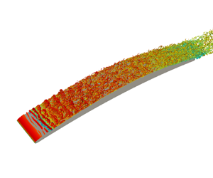
  $12\,\%$ chord; this length is determined to be sufficient to get fully decorrelated turbulence in the span (Moreau & Roger Reference Moreau and Roger2005; Wang et al. Reference Wang, Moreau, Iaccarino and Roger2009; Wu et al. Reference Wu, Moreau and Sandberg2019). The locations of the experimental wall-pressure probes considered over the suction side of the CD aerofoil are along the streamwise direction as shown in figure 1. Sensors $7$ and $9$ are approximately located at mid chord and sensors $21$ and $24$ near the TE.

Figure 1. Remote microphone probes locations on the CD aerofoil. Numbers show sensor indices designated in Wu et al. (Reference Wu, Moreau and Sandberg2019).
The mean pressure distribution over the surface of the CD aerofoil is analysed in figure 2 through the mean wall-pressure coefficient distribution,
 \begin{equation} -C_p =-\frac{\bar{p}-p_{\infty}}{\frac{1}{2}\rho U^{2}_{\infty}}, \end{equation}
where  $p_{\infty }$ and $\rho$ are the reference static pressure and air density taken at the inlet respectively. The mean wall-pressure coefficient calculated from the DNS is also compared with wall-pressure measurements by Jaiswal et al. (Reference Jaiswal, Moreau, Avallone, Ragni and Pröbsting2020) and Jaiswal (Reference Jaiswal2020), taken at several locations over the suction and pressure side of the CD aerofoil. As shown in figure 2, a small plateau between $x/c=-1$ and $x/c=-0.9$ indicates a small laminar recirculation bubble at the aerofoil LE that triggers the transition to turbulence in the bubble shear layer and consequently an attached turbulent flow. After the reattachment point, the pressure gradient increases along the CD aerofoil. The flow is first subjected to a FPG, then to a ZPG around mid-chord and finally to an APG downstream due to the aerofoil camber. On the pressure side, the flow is laminar and attached until the TE where it transitions to turbulence with a small vortex shedding appearing in the near wake, mixing with the turbulent flow on the suction side (Neal Reference Neal2010; Moreau et al. Reference Moreau, Sanjosé, Pérot and Kim2011; Wu et al. Reference Wu, Sanjose, Moreau and Sandberg2018). By comparison with the set of experimental data produced at UdeS (Jaiswal Reference Jaiswal2020; Jaiswal et al. Reference Jaiswal, Moreau, Avallone, Ragni and Pröbsting2020), the DNS distribution gives a good prediction of the pressure coefficient on the aerofoil, except for a slightly higher pressure plateau within the thin LSB at the LE (Wu et al. Reference Wu, Moreau and Sandberg2020), see figure 2.

Figure 2. Pressure coefficient distribution,  $C_p$, on the CD aerofoil: ——, DNS (Wu et al. Reference Wu, Moreau and Sandberg2019); $\bullet$, experiment (Jaiswal Reference Jaiswal2020; Jaiswal et al. Reference Jaiswal, Moreau, Avallone, Ragni and Pröbsting2020).
As shown in figure 1, the four points of the aerofoil suction side analysed correspond to ZPG (sensors  $7$ at $x/c=-0.60$ and $9$ at $x/c=-0.47$) and APG (sensors $21$ at $x/c=-0.14$ and $24$ at $x/c=-0.08$) locations. For each location, a volume of data containing the pressure and velocity distributions is extracted.
2.1. Signal processing
A summary of the signal processing adopted throughout the paper is presented here. The DNS volume data are appropriately scaled to obtain dimensional quantities. In particular, the numerical pressure data are rescaled by  $\rho U^{2}_{\infty }$. The wall-pressure statistics are then computed for the four locations corresponding to sensors $7, 9, 21$ and $24$.
$24$.
For all four sensor locations and even for those close to the TE in the strong APG region, the local pressure field has been found homogeneous in planes parallel to the wall and stationary in time, both numerically (Grasso et al. Reference Grasso, Jaiswal, Wu, Moreau and Roger2019) and experimentally (Jaiswal Reference Jaiswal2020; Jaiswal et al. Reference Jaiswal, Moreau, Avallone, Ragni and Pröbsting2020). In practical applications, only single time histories of the stochastic variable are available, and thus the stationary process is normally assumed to be ergodic. Under such conditions, the space–time cross-correlation function of the wall-pressure fluctuations  $p'=p-\bar {p}$ at two arbitrary space–time points is defined as
 \begin{equation} R_{pp}(\boldsymbol{\xi}; \tau) = \lim_{T \rightarrow \infty} \frac{1}{T} \int^{T}_0 p'(\boldsymbol{x},t) p'(\boldsymbol{x} + \boldsymbol{\xi},t+\tau) \,\mathrm{d}t, \end{equation}
where  $\boldsymbol {\xi }$ is the spatial separation vector between two points located at $\boldsymbol {x}$ and $\boldsymbol {x} + \boldsymbol {\xi }$ with time delay $\tau$. In this way, the random sample in space and time is compressed into a much shorter function of $\boldsymbol {\xi }$ and $\tau$. The cross-spectral density (CSD) is then calculated with a simple fast Fourier transformation using a Welch periodogram technique and Hanning windowing with zero padding (Salze et al. Reference Salze, Bailly, Marsden, Jondeau and Juvé2014),
 \begin{equation} \varPsi_{pp}(\boldsymbol{\xi};\omega) = \frac{1}{2{\rm \pi}} \int^{\infty}_{-\infty} R_{pp}(\boldsymbol{\xi}, \tau) \exp (-\mathrm{i}\omega \tau) \,\mathrm{d}\tau. \end{equation}
The spectra are computed using a Welch periodogram method with  $16$ windows, each containing $512$ points, and with $50\,\%$ overlap. The high-frequency numerical noise is filtered out using a Butterworth filter. By doing a two-dimensional (2D) spatial Fourier transform of $\varPsi _{pp}(\boldsymbol {\xi };\omega )$ with the cross-correlation spectra for each time block averaged together, the CSD function in the wavenumber-frequency domain is then computed by discretising the following Fourier integral
 \begin{equation} \varPsi_{pp}(\boldsymbol{k};\omega) = \frac{1}{(2{\rm \pi})^2} \int\int^{\infty}_{-\infty} \varPsi_{pp}(\boldsymbol{\xi};\omega) \exp (-\mathrm{i}\boldsymbol{k} \boldsymbol{\xi})\, \mathrm{d}\boldsymbol{\xi}, \end{equation}
where  $\boldsymbol {k}=(k_x,k_z)$ is the 2D wavevector (Bull Reference Bull1996), with $k_x$ and $k_z$ the streamwise and spanwise wavenumbers, respectively. The PSD or single-point wall-pressure spectrum (i.e. auto-spectrum), $\phi _{pp}$, at a given angular frequency $\omega$, is related to the space–time correlation function and the wavenumber-frequency spectrum by
 \begin{align} \phi_{pp}(\omega)& = \frac{1}{2{\rm \pi}} \int^{\infty}_{-\infty} R_{pp}(0;\tau) \exp (-\mathrm{i}\omega \tau) \,\mathrm{d}\tau,\nonumber\\ & = \int\int^{\infty}_{-\infty}\varPsi_{pp}(\boldsymbol{k};\omega)\,\mathrm{d}\boldsymbol{k}. \end{align}
The resolved normalised frequency range is  $0\leq \omega \delta ^{*}/U_{\infty }\leq 5.53$ (where $\delta ^*$ is the boundary layer displacement thickness) with a frequency resolution of $\Delta \omega =1.4\times 10^{-3}U_{\infty }/\delta ^{*}$ and a wavenumber resolution of $\Delta k_x=0.12/\delta ^{*}$ in the streamwise direction and $\Delta k_z=0.14/\delta ^{*}$ in the spanwise direction.
3. Boundary layer development
The TBL characteristics calculated from the DNS data on the aerofoil suction side of figure 1 are shown and discussed here. These distributions are compared with results of several available numerical and experimental data sets (Schloemer Reference Schloemer1967; Brooks & Hodgson Reference Brooks and Hodgson1981; Spalart Reference Spalart1988; Watmuff Reference Watmuff1989; Na & Moin Reference Na and Moin1998; Schlatter et al. Reference Schlatter, Li, Brethouwer, Johansson and Henningson2009a,Reference Schlatter, Örlü, Li, Brethouwer, Fransson, Johansson, Alfredsson and Henningsonb; Vinuesa et al. Reference Vinuesa, Hosseini, Hanifi, Henningson and Schlatter2017; Cohen & Gloerfelt Reference Cohen and Gloerfelt2018; Tanarro et al. Reference Tanarro, Vinuesa and Schlatter2020; Hu Reference Hu2021).
In table 1, the properties of the TBL for the current DNS at the four sensors locations are summarised. The flow properties for DNS cases of Choi & Moin (Reference Choi and Moin1990), Spalart (Reference Spalart1988), Tanarro et al. (Reference Tanarro, Vinuesa and Schlatter2020) and Na & Moin (Reference Na and Moin1998) (including both ZPG TBL,  $x=0.50$, attached APG TBL, $x=0.85$, and separated APG TBL at $x/\delta _{in}^{*}=120$) are also reported in table 1. In addition, the ZPG, APGs and APGw cases of Cohen & Gloerfelt (Reference Cohen and Gloerfelt2018) are also included in table 1. These data are also considered later for comparison of PSD and the convection velocities.
Table 1. Properties of the TBL for the current DNS data and for several existing studies in the literature.

Here,  ${Re}_{\tau }=u_{\tau } \delta /\nu \equiv \delta ^+$ is the friction Reynolds number or Kármán number, with $u_{\tau }=\sqrt {\tau _{w}/\rho }$ the friction velocity, $\tau _{w}=\mu ({\partial U}/{\partial y})|_{y=0}$ the wall shear stress ( $U$ is the streamwise mean velocity component and $y$ is the wall-normal distance from the wall) and $\delta$ the boundary layer thickness. The latter is calculated based on the conservation of the stagnation pressure $p_{t}=\rho u^{2}_{t}/2 +p_{\infty }$ outside the boundary layer for the present low-speed flow; $u^{2}_{t}$ is the velocity magnitude squared. The edge of the boundary layer is considered reached when $p_t$ is $95\,\%$ of its maximum value in the wall-normal direction (Sanjosé & Moreau Reference Sanjosé and Moreau2018; Griffin, Fu & Moin Reference Griffin, Fu and Moin2021). This criterion was also used in the boundary-layer data extraction by Christophe et al. (Reference Christophe, Moreau, Hamman, Witteveen and Iaccarino2015); the criterion is necessary as the edge velocity is not constant around the aerofoil in the jet potential core. Here $\beta _c=\delta ^{*}/ \tau _{w}({\rm d}p/{\rm d}s)$ is the Clauser parameter, with ${\rm d}p/{\rm d}s$ the streamwise mean pressure gradient on the wall. The acceleration parameter is $K=\nu / U^{2}_{e}({\rm d}U_{e}/{\rm d}s)$ and $H= \delta ^*/\theta$ is the shape factor. Both $\beta _c$ and $K$ vary strongly along the curvilinear abscissa $s$, which confirms a strongly non-equilibrium TBL on the CD aerofoil suction side according to criterion (iii). To quantify this non-equilibrium state, in figure 3, the evolution of $\beta _c$ as a function of the defect shape factor $G\equiv [(H-1)/H] u_{\tau }/U_e$ or the friction Reynolds number ${Re}_{\tau }$ is shown for the current case and compared with the theoretical equilibrium turbulent boundary-layer data of Mellor & Gibson (Reference Mellor and Gibson1966), the quasi-equilibrium cases corresponding to constant and varying $\beta _c$ simulated by Bobke et al. (Reference Bobke, Vinuesa, Örlü and Schlatter2017) ( $m$ in caption is the power-law exponent of varying streamwise velocity at the top boundary to yield near-equilibrium APG flow conditions, based on definition by Townsend (Reference Townsend1961)), and the non-equilibrium flow data from NACA0012 and NACA4412 aerofoils (Tanarro et al. Reference Tanarro, Vinuesa and Schlatter2020). The present simulation is noticeably further away from the theoretical equilibrium $G$-factor and presents a faster growth of $\beta _c$, yielding a TBL on the verge of separation for Kármán numbers typical of highly loaded low-speed fans.

Figure 3. Clauser pressure-gradient parameter  $\beta _c$ as function of (a) defect shape factor $G$ and (b) friction Reynolds number ${Re}_{\tau }$. $-\,{\cdot }\,-$, present CD aerofoil DNS; — (light blue), theoretical equilibrium data (Mellor & Gibson Reference Mellor and Gibson1966); flat plate DNS for constant and non-constant $\beta _c$-cases (Bobke et al. Reference Bobke, Vinuesa, Örlü and Schlatter2017): — (green), $m=-0.13$ with $\beta _c=[0.86; 1.49]$, — (blue), $m=-0.16$ with $\beta _c=[1.55; 2.55]$, — (purple), $m=-0.18$ with $\beta _c=[2.15; 4.07]$, — (orange), $\beta _c=1$ and —- (olive) $\beta _c=2$; — (red) NACA4412 and — (black) NACA0012 aerofoil DNS (Tanarro et al. Reference Tanarro, Vinuesa and Schlatter2020).
The normalised velocity profiles for the current DNS case are presented in figure 4. The profiles obtained at mid-chord locations are similar. Near the TE, a thicker boundary layer with a lower wall shear stress  $\tau _{w}$ is observed, due to APG.

Figure 4. Dimensionless velocity profiles: ZPG locations  $x/c=-0.60$ (thin grey line) and $x/c=-0.47$ (thick grey line); APG locations $x/c=-0.14$ (thin black line), $x/c=-0.08$ (thick black line).
In figure 5, the skin-friction coefficient,  $C_f=\tau _w/(0.5 \rho U^{2}_{e})$, and the shape factor, $H$, are plotted against Reynolds number based on momentum thickness. The skin-friction coefficient decreases with higher ${Re}_\theta$ as the boundary layer develops. Also shown are the empirical correlation based on the $1/7$ power law of the form $C_f = 0.024 {Re}_{\theta }^{1/4}$ by Smits et al. (Reference Smits, Matheson and Joubert1983), aerofoil data by Vinuesa et al. (Reference Vinuesa, Hosseini, Hanifi, Henningson and Schlatter2017) and Tanarro et al. (Reference Tanarro, Vinuesa and Schlatter2020), and additional reference data (Spalart Reference Spalart1988; Na & Moin Reference Na and Moin1998; Schlatter et al. Reference Schlatter, Li, Brethouwer, Johansson and Henningson2009a,Reference Schlatter, Örlü, Li, Brethouwer, Fransson, Johansson, Alfredsson and Henningsonb; Cohen & Gloerfelt Reference Cohen and Gloerfelt2018). In the ZPG zone around ${Re}_{\theta }=320$, the skin-friction coefficient and the shape factor matches well with the correlation values (Monkewitz et al. Reference Monkewitz, Chauhan and Nagib2007; Schlatter & Örlü Reference Schlatter and Örlü2010). At higher ${Re}_{\theta }$, the trend of $C_f$ and $H$ with ${Re}_{\theta }$ starts to differ: $C_f$ decreases and $H$ increases much faster in comparison to ZPG correlations. This is caused by the strong APG effects of this highly non-equilibrium flow as the TE is approached. Such a variation is qualitatively inline with previous notable studies on aerofoils (Vinuesa et al. Reference Vinuesa, Hosseini, Hanifi, Henningson and Schlatter2017; Tanarro et al. Reference Tanarro, Vinuesa and Schlatter2020), but with a stronger APG on the verge of separation, typical of highly loaded low-speed fans. The $C_f$ corrected with $(1+\beta _c/10)$ as proposed by Volino (Reference Volino2020) is plotted in figure 5(b). This correction with the Clauser pressure gradient parameter improves the $C_f$ correlation, and collapses all aerofoil data. However, a scatter (though reduced) is still present considering both airfoil and ZPG data, as shown by the current DNS results with modified Volino (Reference Volino2020) corrections with different $\beta _c$ multipliers of 0.12 and 0.15. Therefore, the constant of 0.1 used by Volino (Reference Volino2020) is not universal and depends on the mean pressure gradient. Figure 6 shows the streamwise variations of $\delta$, $\delta ^{*}$ and $\theta$ normalised by $c$, compared with laminar and turbulent flat plate ZPG boundary layer solutions, obtained assuming fully laminar or fully TBL from the LE. In figure 6(a), a hump of $\delta /c$ near the LE is shown as the LSB develops; after the hump, the boundary layer thickness over the CD aerofoil increases after the transition to turbulence, noticeably so around $x/c=-0.6$ in the ZPG region, where $\delta /c$ matches the ZPG turbulent flat plate boundary layer solution. The red dotted box in figure 6(a) represents the aerofoil region considered in figure 6(b–d), which starts around mid-chord at sensor 7 ( $x/c=-0.6$).

Figure 5. (a) Skin friction coefficient,  $C_f$, (b) corrected with $(1+\beta _c/10)$ and (c) shape factor, $H$, versus momentum-thickness-based Reynolds number: $-\,{\cdot }\,-$ (black), DNS data on the surface of the CD aerofoil, $-\,{\cdot }\,-$ (blue), $C_f(1+0.12\beta _c)$, $-\,{\cdot }\,-$ (red), $C_f(1+0.15\beta _c)$, APG locations $\triangledown$, $x/c=-0.14$ and $\boldsymbol {\pmb {+}}$, $x/c=-0.08$; $\, {\cdot }\, {\cdot }\, {\cdot }\, $, empirical correlation by Smits, Matheson & Joubert (Reference Smits, Matheson and Joubert1983) for $C_f$ and correlation form by Monkewitz, Chauhan & Nagib (Reference Monkewitz, Chauhan and Nagib2007) for $H$;
$H$;  $\circ$, NACA4412 data by Vinuesa et al. (Reference Vinuesa, Hosseini, Hanifi, Henningson and Schlatter2017); $\blacksquare$, NACA4412 data by Tanarro et al. (Reference Tanarro, Vinuesa and Schlatter2020); $+$, data by Spalart (Reference Spalart1988); and $\bullet$, data by Schlatter et al. (Reference Schlatter, Li, Brethouwer, Johansson and Henningson2009a,Reference Schlatter, Örlü, Li, Brethouwer, Fransson, Johansson, Alfredsson and Henningsonb); $\blacktriangle$, FPG (blue), ZPG (black), APGs (red) and APGw (magenta) data by Cohen & Gloerfelt (Reference Cohen and Gloerfelt2018); $\,{\cdot }\,{\cdot }\,{\cdot }\,$ (red) attached TBL distribution by Na & Moin (Reference Na and Moin1998); $\triangle$, data ( $x=0.5$ m to $x=0.85$ m) for attached TBL (black) and separated TBL (red) ( $x/\delta _{in}^*=120$) by Na & Moin (Reference Na and Moin1998).

Figure 6. Normalised boundary layer parameters distribution on the surface of the CD aerofoil: (a,b) boundary layer thickness based on  $95\,\%$ of total pressure; (c) boundary layer displacement thickness; and (d) boundary layer momentum thickness; $\,{\cdot }\,{\cdot }\,{\cdot }\,$, laminar flat plate; and $-\,{\cdot }\,-$, turbulent flat plate (Schlichting & Gersten Reference Schlichting and Gersten2017).
The boundary layer displacement thickness (figure 6c) and the boundary layer momentum thickness (figure 6d) are obtained by integration of the corresponding velocity profile across the boundary layer,
 \begin{equation} \delta^{*}(x) = \int^{\delta}_{y=0} \left(1-\frac{U}{U_e}\right) \,\mathrm{d} y,\quad \theta(x) = \int^{\delta}_{y=0}\frac{U}{U_e} \left(1-\frac{U}{U_e}\right) \,\mathrm{d} y. \end{equation}
The increasing growth rate of the boundary layer as shown by all three thicknesses is due to the APG experienced by the boundary layer as it develops in the aft portion of the CD aerofoil. The departure from ZPG turbulent solutions is consistent with the fact that the TBL is subjected to strongly non-equilibrium APG. In figure 7, the variations of  $\delta ^{*}/\delta _{in}^{*}$ and $\theta /\theta _{in}$ in the APG region are plotted versus the momentum-thickness-based Reynolds number, together with the turbulent flat plate solution (black dotted-dashed line). Such a normalisation is consistent with that of Na & Moin (Reference Na and Moin1998) and Cohen & Gloerfelt (Reference Cohen and Gloerfelt2018) (also shown in figure 7); the subscript ‘ $in$’ indicates quantities at an upstream ZPG location. For the present DNS, the ‘ $in$’ location is taken at the location $x/c=-0.6$ (i.e. sensor $7$). The present boundary-layer growth on the CD aerofoil is much faster than in the equilibrium cases of Na & Moin (Reference Na and Moin1998) and Cohen & Gloerfelt (Reference Cohen and Gloerfelt2018), and only the separated TBL case in Na & Moin (Reference Na and Moin1998) displays similar rapid increase of boundary layer thicknesses, stressing again the strong non-equilibrium state near the TE close to flow separation. Streamwise mean velocity profiles scaled on inner variables $U^{+}=U/u_{\tau }$ are plotted versus the normalised wall-normal distance $y^{+}=yu_{\tau }/\nu$ in figure 8. The present DNS results are compared with the DNS data by Spalart (Reference Spalart1988) at ${Re}_{\theta }=300$, Na & Moin (Reference Na and Moin1998) for $x=0.5$ m and $x=0.85$ m, Cohen & Gloerfelt (Reference Cohen and Gloerfelt2018), as well as the experimental data of Watmuff (Reference Watmuff1989) for $x=0.5$ and $x=0.85$. Figure 8(a) compares the ZPG data, whereas figure 8(b) considers the APG data. The von Kármán constant $\kappa$ (von Kármán Reference von Kármán1931) and the constant $B$ are prescribed as in Wu et al. (Reference Wu, Moreau and Sandberg2019): $\kappa =0.41$ and $B=4.5$ for the ZPG cases, and $\kappa =0.30$ and $B=-1.38$ for the APG cases. Wu et al. (Reference Wu, Moreau and Sandberg2019) showed that an attached APG flow is characterised by lower $\kappa$ values than in a ZPG flow, as well as a negative intercept ( $B$) value, consistently with what Nickels (Reference Nickels2004), Nagib & Chauhan (Reference Nagib and Chauhan2008) and Monty et al. (Reference Monty, Harun and Marusic2011) found, for instance. The present ZPG profiles compare well with the ZPG data of Spalart (Reference Spalart1988), Na & Moin (Reference Na and Moin1998) and Watmuff (Reference Watmuff1989). Moving towards the TE, a stronger wake region is observed due to APG effect, as also observed in previous studies (Monty et al. Reference Monty, Harun and Marusic2011; Kitsios et al. Reference Kitsios, Atkinson, Sillero, Borrell, Gungor, Jiménez and Soria2016; Bobke et al. Reference Bobke, Vinuesa, Örlü and Schlatter2017; Vila et al. Reference Vila, Örlü, Vinuesa, Schlatter, Ianiro and Discetti2017; Volino Reference Volino2020).

Figure 7. Normalised boundary layer parameters distribution versus momentum-thickness-based Reynolds number. (a) Boundary layer displacement thickness and (b) boundary layer momentum thickness: —, DNS data on the surface of the CD aerofoil;  $\blacktriangle$, FPG (blue), ZPG (black), APGs (red), APGw (magenta) data by Cohen & Gloerfelt (Reference Cohen and Gloerfelt2018); $\,{\cdot }\,{\cdot }\,{\cdot }$ (red) attached TBL distribution by Na & Moin (Reference Na and Moin1998); $\triangle$, data ( $x=0.5$ m to $x=0.85$ m) for attached TBL (black) and separated TBL (red) ( $x/\delta _{in}^{*}=120$) by Na & Moin (Reference Na and Moin1998); $-\,{\cdot }\,-$, turbulent flat plate (Schlichting & Gersten Reference Schlichting and Gersten2017).

Figure 8. Streamwise velocity profiles as a function of the wall-normal distance scaled on inner variables: (a) ZPG profile and (b) APG profile. Present DNS: ZPG locations  $x/c=-0.60$ (thin grey line) and $x/c=-0.47$ (thick grey line); APG locations $x/c=-0.14$ (thin black line), $x/c=-0.08$ (thick black line). Symbols: $+$, ZPG data by Spalart (Reference Spalart1988) with ${Re}_{\theta }=300$; $--$, ZPG data $x=0.5$ m (black) and APG data $x=0.85$ m (red) data by Watmuff (Reference Watmuff1989); $\circ$, ZPG data $x=0.5$, $\square$, APG data $x=0.85$ for attached TBL (black) and separated TBL $x/\delta _{in}^{*}=130$ (grey) by Na & Moin (Reference Na and Moin1998); $\triangle$, ZPG (black), APGs (red) and APGw (magenta) data by Cohen & Gloerfelt (Reference Cohen and Gloerfelt2018); $\,{\cdot }\,{\cdot }\,{\cdot }\, $, dimensionless linear law $U^{+}=y^{+}$ and $-\,{\cdot }\,-$, logarithmic law $U^{+}=({1}/{\kappa })\ln (y^{+})+B$.
In figure 9, wall-normal profiles of root-mean-square (r.m.s.) streamwise and crosswise velocities,  $u_{rms}$ and $v_{rms}$, scaled with inner variables, with $U_e$, and with the Zaragola–Smits scaling $U_{ZS}=U_{e}\delta ^{*}/\delta$ are shown for the four sensor locations, compared with the ZPG data of Spalart (Reference Spalart1988) and both the ZPG and APG data of Na & Moin (Reference Na and Moin1998) and Cohen & Gloerfelt (Reference Cohen and Gloerfelt2018). Figures 9(a,b) show profiles of $u_{rms}$ and $v_{rms}$ normalised by $u_{\tau }$. A slightly higher peak for $u^{+}_{rms}$ in sensors $7$ and $9$ in comparison with Spalart (Reference Spalart1988) can be attributed to the FPG region prior to those streamwise locations. The higher $u^{+}_{rms}$ and $v^{+}_{rms}$ in APG region than in ZPG region is mainly because of the decrease of wall friction (figure 5). The smaller wall friction in the present DNS than in the reference studies (associated with stronger APG herein) also explains the larger $u_{rms}^+$ and $v_{rms}^+$ peaks in the present study. The inner peak elevations remain almost unchanged. Yet, a second peak forms in the outer layer in the $u_{rms}$ profile. The differences between the outer-peak locations (in wall units) in the present case and in the studies of Na & Moin (Reference Na and Moin1998) and Cohen & Gloerfelt (Reference Cohen and Gloerfelt2018) are most likely attributed to a combination of differences in APG, Reynolds number and wall curvature. An effect of Reynolds number on the outer-layer peak location was discussed by Lee & Sung (Reference Lee and Sung2008), for instance. In figure 9(c,d), the outer-layer velocity fluctuations normalised by $U_e$ display large deviation from each other, and only collapse at the boundary-layer edge. However, when the APG cases are normalised by $U_{ZS}$ (figure 9e,f), the outer-layer velocity fluctuations are almost collapsed. This suggests that the Zaragola–Smits scaling applies to the outer portion of the boundary layer even under strong APG as in the present flow. This is consistent with the self-similarity in the outer region of APG TBL found by Maciel, Rossignol & Lemay (Reference Maciel, Rossignol and Lemay2006), Cohen & Gloerfelt (Reference Cohen and Gloerfelt2018) and also verified by Rozenberg, Robert & Moreau (Reference Rozenberg, Robert and Moreau2012) to develop their semi-empirical model of wall-pressure fluctuations.

Figure 9. Comparison of r.m.s. velocities  $u_{rms}$ and $v_{rms}$, in the wall-normal direction: (a,b) $u_{\tau }$ scaling; (c,d) $U_{e}$ scaling; (e,f) $U_{ZS}=U_{e}\delta ^{*}/\delta$ scaling. ZPG locations $x/c=-0.60$ (thin grey line) and $x/c=-0.47$ (thick grey line); APG locations $x/c=-0.14$ (thin black line), $x/c=-0.08$ (thick black line). Symbols: $+$, ZPG data by Spalart (Reference Spalart1988) with ${Re}_{\theta }=300$; $\circ$, ZPG data $x=0.5$ m, $\square$, APG data $x=0.85$ m, for attached TBL (black) by Na & Moin (Reference Na and Moin1998); $\triangle$, ZPG (black), APGs (red) and APGw (magenta) data by Cohen & Gloerfelt (Reference Cohen and Gloerfelt2018).
The wall-normal profiles of Reynolds shear stress in inner scaling at the four streamwise locations are plotted in figure 10. In the ZPG region, the profiles compare well with that of Spalart (Reference Spalart1988); the same is observed for the  $u'$ and $v'$ intensities (figure 9a,b). The peaks of the Reynolds shear stress shift away from the wall in the APG region, moving into the logarithmic layer and even toward the edge of the outer region. This indicates enhanced turbulent mixing at locations farther away from the wall (Monty et al. Reference Monty, Harun and Marusic2011; Vila et al. Reference Vila, Örlü, Vinuesa, Schlatter, Ianiro and Discetti2017; Wu et al. Reference Wu, Moreau and Sandberg2019). As discussed by Lee & Sung (Reference Lee and Sung2008), who analysed the effect of APG with similar ${Re}_{\theta }$, the plateau observed so far for the strongest APG for $y^+$ between 10 and 50 may be due to the hairpin-type vortices developing away from the wall next to the TE region, also shown in the present DNS in figure 11, which shows the swirling strength criterion ( $\varLambda _{ci}$) in the mid-chord (ZPG) region and near the TE (APG region). A forest of large hairpin structures are shown to be lifted by the strong APG (see white dotted lines). Therefore, the APG, characterised by a different momentum distribution mechanisms across the boundary layer, considerably affects the turbulent flow statistics (figure 10).

Figure 10. Reynolds stress component normalised with inner scale along wall-normal direction: ZPG locations  $x/c=-0.60$ (thin grey line) and $x/c=-0.47$ (thick grey line); APG locations $x/c=-0.14$ (thin black line), $x/c=-0.08$ (thick black line); $+$, ZPG data by Spalart (Reference Spalart1988) with ${Re}_{\theta }=300$.

Figure 11. Swirling strength criterion (Zhou et al. Reference Zhou, Adrian, Balachandar and Kendall1999; Wu et al. Reference Wu, Moin, Wallace, Skarda, Lozano-Durán and Hickey2017) isocontours coloured by streamwise velocity component by Wu et al. (Reference Wu, Moreau and Sandberg2019): (a) ZPG portion (mid-chord) and (b) APG (or TE) portion.
The results above show that boundary layer characteristics and single-point velocity statistics at the four sensor locations are consistent with existing results in the literature. The agreements are quantitative at the ZPG locations. Overall, the peak location of the turbulent statistics and the wall-normal profiles are comparing very well with Spalart (Reference Spalart1988) (see grey lines up to  $y^{+}\approx 60$ in figures 9 and 10). The agreement is qualitative at the APG locations because of the different Reynolds numbers, pressure gradients and wall curvature. Interestingly, the self-similarity in the outer region of the boundary layer provided by the Zaragola–Smits scaling is verified in the present strong non-equilibrium TBL, suggesting that the Zaragola–Smits velocity might be a relevant velocity scale for all attached TBL. The discussion on variation of boundary layer parameters serves as a guide on normalising wall-pressure statistics. For instance, turbulence statistics, when made dimensionless by Zaragola–Smits scaling, gives a collapse in outer region and thus may serve as an optimal velocity scale to collapse low-frequency wall-pressure spectra. The development of boundary layer thicknesses discussed in figure 6 can also guide in choosing the correct normalising length scale for wall-pressure spectra in highly non-equilibrium cases. Moreover, the high sensitivity of $C_f$ to APG, more aptly wall shear, suggests that it may not be an optimal parameter to non-dimensionalise pressure fluctuations, even though most semi-empirical models for wall-pressure spectra use it as a pressure scale. This is shown in detail in the next section.
4. Wall-pressure statistics
Statistics of the wall-pressure field on the surface of the CD aerofoil particularly relevant to TE noise modelling are presented here. PSD, two-point correlation, coherence functions, wavenumber-frequency spectra and convection velocity are discussed at the four locations corresponding to sensors  $7, 9, 21$ and $24$. They are compared with available data (Burton Reference Burton1973; Schewe Reference Schewe1983; Simpson et al. Reference Simpson, Ghodbane and McGrath1987; Spalart Reference Spalart1988; Choi & Moin Reference Choi and Moin1990; Na & Moin Reference Na and Moin1998; Skote, Henningson & Henkes Reference Skote, Henningson and Henkes1998; Abe et al. Reference Abe, Matsuo and Kawamura2005; Cohen & Gloerfelt Reference Cohen and Gloerfelt2018).
4.1. PSD distribution
The PSD of the wall-pressure fluctuations at a given frequency,  $\phi _{pp}(\,{f})$, is calculated from the wall-pressure CSD, as defined in § 2.1. The spanwise-averaged wall-pressure spectra in decibels with respect to the reference pressure $2\times 10^{5}$ Pa for a spectral resolution of 1 Hz ( ${\rm dB}\,{\rm Hz}^{-1}$ in short) are shown in figure 12 for the four locations on the aerofoil suction side indicated in figure 1. The PSD calculated from DNS are compared with the available experimental data from UdeS measurements (Jaiswal Reference Jaiswal2020; Jaiswal et al. Reference Jaiswal, Moreau, Avallone, Ragni and Pröbsting2020). Note that the experimental results for sensor $7$ are missing because of a microphone failure. In figures 12(a,b), for the ZPG regions $7$ and $9$, the semi-empirical spectrum defined by Goody (Reference Goody2004) is also represented. Such a model compares well with experimental data over a large range of Reynolds numbers (Hwang, Bonness & Hambric Reference Hwang, Bonness and Hambric2009), and is able to describe the essential properties of the single-point wall-pressure spectrum for ZPG boundary layers based on a limited numbers of variables. Note that at low frequencies, the same $-0.4$ slope is recovered as observed in the APG DNS of Na & Moin (Reference Na and Moin1998). For sensor $24$ (figure 12d) the DNS spectrum shows a small hump around 10 kHz. This hump in the higher-frequency range is also shown in the experimental data (grey line) and corresponds to an extra acoustic source in the wake (Wu et al. Reference Wu, Moreau and Sandberg2020). Going towards the TE, there is an increase in spectral levels of approximately $10\,{\rm dB}\,{\rm Hz}^{-1}$ at the low frequencies, and a faster roll-off decrease towards high frequency. This is an APG effect, also observed in previous studies (Na & Moin Reference Na and Moin1998; Cohen & Gloerfelt Reference Cohen and Gloerfelt2018). In the low-frequency range a plateau below $500$ Hz is observed for sensors $21$ and $24$, whereas sensors $7$ and $9$ show the characteristic ZPG quadratic rise with frequency following Goody's empirical model. Overall, the DNS and experimental results are in good agreement. The difference of PSDs between numerical and experimental results in the low-frequency range, approximately under $500$ Hz, is most likely related to installation effects, either attributed to jet noise (Moreau et al. Reference Moreau, Henner, Iaccarino, Wang and Roger2003) or to the unsteady interaction between the jet shear layer and the aerofoil, as well as the low background turbulence intensity (less than 0.4 %) observed in the experiments (Padois et al. Reference Padois, Laffay, Idier and Moreau2015) and not included in this DNS (Wu et al. Reference Wu, Moreau and Sandberg2020).

Figure 12. Spanwise-averaged wall-pressure spectra at four locations on the aerofoil suction side: ——, DNS-NS;  $-\,{\cdot }\,-$, Goody's model, and —— (grey), UdeS measurements; (a) $x/c=-0.60$, (b) $x/c=-0.47$, (c) $x/c=-0.14$ and (d) $x/c=-0.08$.
In order to deduce the main contributors to the wall-pressure fluctuations in different frequency bands, the PSD and the frequency are then normalised based on several inner, outer and mixed scalings in figure 13. Different normalisations have been proposed over the years (Schloemer Reference Schloemer1967; Choi & Moin Reference Choi and Moin1990; Farabee & Casarella Reference Farabee and Casarella1991; Keith, Hurdis & Abraham Reference Keith, Hurdis and Abraham1992; Bull Reference Bull1996; Na & Moin Reference Na and Moin1998; Cipolla & Keith Reference Cipolla and Keith2000). There is no single universal scaling that leads to an acceptable collapse of data in the entire frequency range due to the multiscale nature of turbulence. However, as observed by Bull (Reference Bull1996) for ZPG flows, the wall-pressure fluctuations at low frequencies originate predominately from the outer layer, whereas those at high frequencies, where the spectrum varies as  $\omega ^{-5}$ (Gravante et al. Reference Gravante, Naguib, Wark and Nagib1998; Na & Moin Reference Na and Moin1998; Moreau & Roger Reference Moreau and Roger2005), originate mostly from the buffer layer. Consequently, the wall-pressure PSD scales on outer variables at lower frequencies and inner variables at high frequencies. In the mid-frequency range, a scale-independent overlap region exists, where the PSD is proportional to $\omega ^{-1}$ (Bradshaw Reference Bradshaw1967; Gravante et al. Reference Gravante, Naguib, Wark and Nagib1998). This range is associated with motions in the logarithmic region.

Figure 13. Dimensionless spanwise-averaged wall-pressure spectra at four locations on the aerofoil suction side: (a) inner variables scaling, (b) mixed inner–outer variables scaling and (c,d) outer variables scaling. ZPG locations  $x/c=-0.60$ (thin grey line) and $x/c=-0.47$ (thick grey line); APG locations $x/c=-0.14$ (thin black line), $x/c=-0.08$ (thick black line); $\bullet$, data by Choi & Moin (Reference Choi and Moin1990); $\circ$, ZPG data $x=0.5$ m, and $\square$, APG data $x=0.85$ m for attached TBL by Na & Moin (Reference Na and Moin1998); $\triangle$, ZPG (black), APGs (red) and APGw (magenta) data by Cohen & Gloerfelt (Reference Cohen and Gloerfelt2018).
The best inner variable scaling for the high-frequency range has been found by plotting  $\phi _{pp}(\omega )u^{2}_{\tau }/\tau ^{2}_{w}\nu$ versus $\omega \nu /u^{2}_{\tau }$ and is used in figure 13(a). For the mid-frequency range, a satisfactory data collapse is usually obtained by scaling $\phi _{pp}(\omega )$ using the mixed inner–outer variables, $U_e$, $\delta ^{*}$ and $\tau _{w}$, with dimensionless frequency $\omega \delta ^{*}/U_e$ (Choi & Moin Reference Choi and Moin1990; Keith et al. Reference Keith, Hurdis and Abraham1992; Na & Moin Reference Na and Moin1998). This is shown in figure 13(b). Finally, in figure 13(c,d), common outer variable scalings for the low-frequency range are used: $\phi _{pp}(\omega ) U_e/p^{2}_{rms}\delta ^{*}$ and $\phi _{pp}(\omega ) U_e/q_{e}^{2}\delta ^{*}$, both versus $\omega \delta ^{*}/U_e$ (Choi & Moin Reference Choi and Moin1990; Na & Moin Reference Na and Moin1998). Here, $q_{e}$ is the dynamic pressure at the edge of the boundary layer.
First, the focus is given to the ZPG data sets. Normalisation with inner variables (figure 13a) collapses the spectra at high frequencies as expected, consistently with the findings of Na & Moin (Reference Na and Moin1998) and Choi & Moin (Reference Choi and Moin1990). Moreover, the present spectra at sensors  $7$ and $9$ collapse well in the whole spectral range with that of Choi & Moin (Reference Choi and Moin1990), as the flow is characterised by a similar range of ${Re}_{\theta }$ (see table 1). In figure 13(b), the scaling with $U_e/\tau _{w}^{2} \delta ^*$ gives an overall collapse at low to mid frequencies, which was also observed by Na & Moin (Reference Na and Moin1998), Choi & Moin (Reference Choi and Moin1990) and Cohen & Gloerfelt (Reference Cohen and Gloerfelt2018). In addition, the effect of Reynolds numbers on the PSD is shown. As observed by Goody (Reference Goody2004), the main effect of Reynolds number on the wall-pressure spectrum is to widen its overlap range and shift the roll-off towards higher frequencies. This is indeed shown in figure 13(c,d), comparing data from Cohen & Gloerfelt (Reference Cohen and Gloerfelt2018) with those from Choi & Moin (Reference Choi and Moin1990) and those from sensor 7 to those from sensor 24 at a higher Reynolds number, for example. This is caused by the widening of the spectrum of turbulent motions and a larger logarithmic region associated with a higher-Reynolds-number boundary layer. Furthermore, a region of the spectra with a $-5$ slope in the high-frequency range, linked to the turbulent motions inside the buffer zone, is also shown in figure 13(c).
As the pressure gradient changes from zero to adverse (from sensor  $9$ to sensor $24$), an overall increase in spectral levels normalised by the inner velocity scale is shown in figure 13, suggesting an augmentation of wall-pressure r.m.s. due to the APG, relative to $u_\tau$. In the presence of an APG the inner variables normalisation does not collapse the spectra at high frequencies, consistently with the observations of Na & Moin (Reference Na and Moin1998) and Cohen & Gloerfelt (Reference Cohen and Gloerfelt2018). This is because of the decrease in wall shear stress under APG. When the spectra are normalised by wall-pressure r.m.s. and $\delta ^*$ (figure 13c), a collapse in the low- to mid-frequency range is observed. This is expected because $p_{rms}^2$ represents the integral of the spectrum. The scaling with local dynamic pressure (figure 13d), on the other hand, does not give a good collapse in the low- to mid-frequency range, which is consistent with what Brooks & Hodgson (Reference Brooks and Hodgson1981) observed on the NACA0012 aerofoil (figure 11 in Brooks & Hodgson Reference Brooks and Hodgson1981). This is because the APG leads to augmentation of wall-pressure fluctuations at low frequencies, whereas it is associated with free-stream deceleration, i.e. a reduction in the edge dynamic pressure. Na & Moin (Reference Na and Moin1998) also observed similar comparison between ZPG and APG wall-pressure spectra for the normalisations analysed herein. Given that all cases plotted here differ in Reynolds numbers, pressure gradients and wall curvature, the spectra do not overlap over the entire frequency range. In addition, both ZPG and APG data of Cohen & Gloerfelt (Reference Cohen and Gloerfelt2018) display a faster roll-off at high frequencies, which is most likely a consequence of the spatial cut-off of the LES. These results also indicate that scalings used in popular semi-empirical models, especially using wall shear stress as the pressure scale, may be inappropriate for strong APG flows.
In figure 14, the pressure spectra are plotted again normalised using  $\delta$ instead of $\delta ^{*}$, which is equivalent to using the Zaragola–Smits scaling instead of $U_{e}$ in figure 13 (because $\omega \,\delta /U_e=\omega \,\delta ^*/U_{ZS}$ and $U_e/\delta =U_{ZS}/\delta ^*$). ZPG and APG data of Cohen & Gloerfelt (Reference Cohen and Gloerfelt2018) for which all parameters are available are also shown. As shown by figure 6(b,c) and also indicated by Keith et al. (Reference Keith, Hurdis and Abraham1992) and Farabee & Casarella (Reference Farabee and Casarella1991), $\delta$ and $\delta ^{*}$ are not equivalent length scales given that their ratio varies with Reynolds number. For the outer scaling, both figure 14(a,b) show a significantly improved collapse compared with figure 13(c,d). This indicates that $\delta$ is a better length scale in the low- to mid-frequency range than $\delta ^*$, or equivalently that $U_{ZS}$ is a better velocity scale than $U_e$. Similarly, for the mixed inner–outer variable scaling, figure 14(c) shows a slightly better merge of the normalised spectra at mid-to-high frequencies for both ZPG and APG regions than in figure 13(b). Finally, the best overall collapse of normalised spectra in the whole frequency range is found in figure 14(a), which stresses that $p_{rms}$ is a better pressure scale than $q_{e}$ for the present highly non-equilibrium TBL. Hence, in development of wall-pressure spectra models, more focus is needed on modelling pressure gradient effects on $p_{rms}$ or on variables that scale with it.

Figure 14. Spanwise-averaged wall-pressure spectra at four locations on the aerofoil suction side scaled with Zaragola–Smits scaling,  $U_{ZS}=U_{e}\delta ^{*}/\delta$: ZPG locations $x/c=-0.60$ (thin grey line) and $x/c=-0.47$ (thick grey line); APG locations $x/c=-0.14$ (thin black line), $x/c=-0.08$ (thick black line); $\triangle$, ZPG (black), APGs (red), APGw (magenta) data by Cohen & Gloerfelt (Reference Cohen and Gloerfelt2018). (a,b) Outer and (c) mixed inner–outer variables scaling.
In figure 15(a), the wall-pressure r.m.s. normalised by  $\rho U^{2}_{in}$ (where $U_{in}$ is taken equal to the edge velocity at sensor $7$) as a function of wall-normal distance is compared with that of Na & Moin (Reference Na and Moin1998), for both attached and separated TBLs. Three different TBL cases by Na & Moin (Reference Na and Moin1998) are also considered, characterised by ZPG at $x/\delta ^*_{in}=80$, a weak APG at $x/\delta _{in}^{*}=120$ and a stronger APG just after the detachment at $x/\delta ^*_{in}=160$ therein. A local maximum of $p_{rms}$ is observed and both its elevation and magnitude increase as the flow moves downstream (with strengthened APG) in accordance with the trend shown by Na & Moin (Reference Na and Moin1998). Close to the TE (sensors 21 and 24) the levels and the hump size are close to those near the onset of separation in the flow studied by Na & Moin (Reference Na and Moin1998) ( $x/\delta ^*_{in}=160$), highlighting the high load of the present case, consistently with the shape factor shown in figure 5(c) and in table 1. The streamwise increase of the pressure fluctuations at the wall is also shown in figure 15(b), which shows the streamwise distribution of the wall-pressure r.m.s. normalised by the local maximum magnitude of Reynolds shear stress or the local dynamic pressure. There is clearly less streamwise variation of the wall-pressure r.m.s. when normalised with local peak Reynolds shear stress, as also shown by Na & Moin (Reference Na and Moin1998). Thus, the peak Reynolds shear stress magnitude could be a better scaling variable for wall-pressure fluctuations than $U_e^2$ for all APG flows including the present strong non-equilibrium TBL case.

Figure 15. Root-mean-square values of (a) pressure fluctuations r.m.s. along wall-normal direction and (b) streamwise distribution of the wall-pressure r.m.s. normalised with local Reynolds shear stress ( $\,{\cdot }\, {\cdot }\, {\cdot }\, $) or dynamic pressure ( $-\,{\cdot }\,-$). ZPG locations $x/c=-0.60$ (thin grey line) and $x/c=-0.47$ (thick grey line); APG locations $x/c=-0.14$ (thin black line), $x/c=-0.08$ (thick black line). Na & Moin (Reference Na and Moin1998) data: $-\,{\cdot }\,-$, ZPG data at $x=0.5$ m, $--$, APG data at $x=0.85$ m for attached TBL (black); ——, $x/\delta ^*_{in}=80$, $--$
$--$  $x/\delta ^*_{in}=120$, $\,{\cdot }\,{\cdot }\,{\cdot }\, $, $x/\delta ^*_{in}=160$ for separated TBL (red).
In figures 16(a,b) the root-mean-square values of the wall-pressure scaled with  $\tau _{w}$ or the dynamic pressure versus the friction Reynolds number, ${Re}_{\tau }=u_{\tau }\delta /\nu$, are shown at the four locations. In figure 16(c), the CD aerofoil distribution of $p^{+}_{rms}$ is also plotted versus the momentum-thickness-based Reynolds number. ZPG data of Choi & Moin (Reference Choi and Moin1990), DNS data of Abe et al. (Reference Abe, Matsuo and Kawamura2005) and ZPG data of Spalart (Reference Spalart1988), Cohen & Gloerfelt (Reference Cohen and Gloerfelt2018), Skote et al. (Reference Skote, Henningson and Henkes1998) and Schewe (Reference Schewe1983) are considered for comparison of ZPG data. The empirical law of $p^{+}_{rms}$ versus ${Re}_{\tau }$ developed for ZPG flows by Farabee & Casarella (Reference Farabee and Casarella1991) is also plotted in figure 16(a), in which $(\,p^{+}_{rms})^{2}= 6.5+1.86\ln ({Re}_{\tau }/333)$ for ${Re}_{\tau }>333$ and $(\,p^{+}_{rms})^{2}= 6.5$ for ${Re}_{\tau }\leq 333$. For APG flows, data of Cohen & Gloerfelt (Reference Cohen and Gloerfelt2018), Simpson et al. (Reference Simpson, Ghodbane and McGrath1987) and Burton (Reference Burton1973) are compared here. The data show that $p^{+}_{rms}$ weakly increases with ${Re}_\tau$ in ZPG flows following the empirical law proposed by Farabee & Casarella (Reference Farabee and Casarella1991). For APG flows, a greater scatter is observed, particularly in figure 16(a) (see APG locations $x/c=-0.14$ and $x/c=-0.08$ in the present flow and strong APG data of Burton (Reference Burton1973) and Simpson et al. (Reference Simpson, Ghodbane and McGrath1987)). APG leads to higher $p_{rms}^+$ than in a ZPG flow at the same Reynolds number. In comparison, less scatter is observed in figure 16(b), indicating a better correlation between the wall-pressure r.m.s. and the edge dynamic pressure than that with $\tau _w$. Finally, the sharp increase in $p_{rms}$ with $x$ shown in figure 16 for the present aerofoil further confirms the strong non-equilibrium state of the boundary layer at the TE, subject to a sharp APG.

Figure 16. Root-mean-square values of the wall-pressure r.m.s.: (a)  $\tau _{w}$ scaling and (b) dynamic pressure scaling vs the friction Reynolds number; (c) $\tau _{w}$ scaling versus the momentum-thickness-based Reynolds number. ZPG locations $\circ$, $x/c=-0.60$ and $\square$, $x/c=-0.47$; APG locations $\triangledown$, $x/c=-0.14$ and $\boldsymbol {\pmb {+}}$, $x/c=-0.08$; $\bullet$, Choi & Moin (Reference Choi and Moin1990)'s data; Abe et al. (Reference Abe, Matsuo and Kawamura2005)'s data ( ${\star }$, grey, ${Re}_{\tau }=180$; $\Diamond$, ${Re}_{\tau }=395$; ${\Diamond }$, grey, ${Re}_{\tau }=640$); $\blacktriangleleft$, Spalart (Reference Spalart1988)'s data; $\bigstar$, ZPG (black), APGs (red) and APGw (magenta) data by Cohen & Gloerfelt (Reference Cohen and Gloerfelt2018); $\triangleleft$, Simpson et al. (Reference Simpson, Ghodbane and McGrath1987) APG's data; $\blacktriangle$, Burton (Reference Burton1973) APG's data; $\dots$, empirical law from Farabee & Casarella (Reference Farabee and Casarella1991); $\bullet$ (green), ZPG data by Skote et al. (Reference Skote, Henningson and Henkes1998) ${Re}_{\theta }=350-525$; $-\,{\cdot }\,-$ CD aerofoil distribution; $\blacktriangleleft$ (blue) data by Schewe (Reference Schewe1983).
In summary, the usual inner or inner–outer variable scalings are observed to work in the ZPG regions of the CD aerofoil (despite the possible history effects of the upstream FPG region), but not in the APG regions, with larger departures for higher  $\beta _c$, as found in previous studies. The best scaling parameters are found to be the outer variables $U_e$, $\delta$ and $p_{rms}$ or equivalently $U_{ZS}$, $\delta ^*$ and $p_{rms}$. This indirectly stresses that the overall wall-pressure fluctuations are dominated by the large turbulent scales, the contribution of which increases with higher $\beta _c$. In turn, $p_{rms}$ is observed to scale more with outer variables such as the dynamic pressure $q_e$ than with inner scales such as $\tau _w$. As found previously by Na & Moin (Reference Na and Moin1998) and Abe (Reference Abe2017), for instance, a quasi invariant is obtained when scaling $p_{rms}$ with the local maximum Reynolds shear stress magnitude for the whole range of Reynolds number considered here in a strong non-equilibrium TBL typical of low-speed rotating machines. This has an important implication in choosing correct scalings in wall-pressure spectra models. For instance, most models use the wall shear stress as the pressure scale. However, our results show that $p_{rms}$ or the peak Reynolds shear stress magnitude are more appropriate low-frequency pressure scales. Another important finding is that, for low-Reynolds-number cases such as the current case, using $\delta$ and $U_e$ as length and velocity scales may give good overall collapse of wall-pressure spectra, as shown in figure 14(a).
4.2. Two-point correlations and coherence functions
The contour plots of the two-point correlation functions of wall-pressure fluctuations, introduced in § 2.1, are shown in figure 17 as a function of streamwise ( $\xi _x$) and temporal ( $\Delta t$) separations and normalised with inlet parameters. The slope ${\rm d}(\xi _x)/{\rm d}(\Delta t)$ gives the propagation speed of the eddies, the signatures of which are reflected in wall-pressure fluctuations. As a reference, these slopes of the cross-correlation at each spatial separation found in Na & Moin (Reference Na and Moin1998) flat-plate case of attached TBL, with ZPG at $x=0.50$ m and with APG at $x=0.85$ m, are also indicated by dotted-dashed and dashed red lines, respectively. As expected, a larger propagation speed is observed in the ZPG region, whereas in the APG region the convection speed of the turbulent structures is reduced and the contour plots are broader. This is associated with a longer correlation time of wall-pressure fluctuations in APG region, and it suggests a lower convection velocity of turbulent structures, which are discussed later. Variations of both the slope and broadness of the contours with APG are in agreement with the observations of Na & Moin (Reference Na and Moin1998), despite different ${Re}_{\theta }$ ranges and a stronger APG reached in the present flow.

Figure 17. Contour plot of two-point correlation of wall-pressure fluctuations versus streamwise spatial and temporal separations: (a)  $x/c=-0.60$; (b) $x/c=-0.47$; (c) $x/c=-0.14$; and (d) $x/c=-0.08$. Contour levels are from 0.15 to 0.9 with increments of 0.15. Red lines are collections of outermost point of each iso-contour line for the attached TBL by Na & Moin (Reference Na and Moin1998) to indicate inclinations of the iso-contours: $-\,{\cdot }\,-$ (red), ZPG data at $x=0.5$ m, and $--$ (red), APG data at $x=0.85$ m.
By Fourier transforming the two-point correlation function, the CSD  $\varPsi _{pp}(\boldsymbol {\xi };\omega )$ is calculated (see § 2.1). The cross-spectrum $\varPsi _{pp}(\boldsymbol {\xi };\omega )$ is useful for studying the wall-pressure spatial coherence as a function of frequency (Moreau & Roger Reference Moreau and Roger2005; Roger & Moreau Reference Roger and Moreau2005). In general, the coherence function between two points on the aerofoil surface can be defined as
 \begin{equation} \gamma^{2}(\boldsymbol{\xi};\omega)=\frac{|\varPsi_{pp}(\boldsymbol{\xi};\omega)|^{2}}{\phi_{pp}(\omega)^{2}}. \end{equation}
The coherence function describes the correlation between two points with a spatial separation of  $\xi _x$ in the longitudinal (or streamwise) direction and $\xi _z$ in the lateral (or spanwise) direction at a given frequency. The contours of the calculated coherence distributions are shown along the streamwise and spanwise directions in figures 18 and 19, respectively. On the one hand, both streamwise and spanwise coherence functions are not observed to vary much in the ZPG regions, with a larger coherence in the streamwise direction. On the other hand, the streamwise coherence is observed to be reduced by APG for the whole frequency range, whereas the spanwise coherence overall increases with APG, especially at low frequencies, as already noted by Wang et al. (Reference Wang, Moreau, Iaccarino and Roger2009) based on the first LES on the present aerofoil. Figure 19 also indicates that the spanwise extent of the computational domain (i.e. 0.12 $C$) is sufficient for proper flow development in both ZPG and APG regions for most frequencies beyond 200 Hz, as already pointed out by Wang et al. (Reference Wang, Moreau, Iaccarino and Roger2009) and confirmed experimentally in several test facilities (Moreau & Roger Reference Moreau and Roger2005; Jaiswal Reference Jaiswal2020; Jaiswal et al. Reference Jaiswal, Moreau, Avallone, Ragni and Pröbsting2020). A slight increase of coherence level in the high-frequency range is found for sensor 24, which is caused by an acoustic contamination by an extra noise source in the wake, as already shown in the wall-pressure PSD in figures 12–14 and as mentioned by Wu et al. (Reference Wu, Moreau and Sandberg2020).

Figure 18. Contours of streamwise coherence of fluctuating pressure for ZPG and APG regions: (a)  $x/c=-0.60$; (b) $x/c=-0.47$; (c) $x/c=-0.14$; and (d) $x/c=-0.08$. Symbols: $\cdots$ (red) spatial separations $\xi _x/c=0.007, 0.013 ,0.016$ used in figures 20 and 21; $-\,{\cdot }\,-$ (blue) frequencies of 1600 and 5000 Hz used in figure 22 and 23.

Figure 19. Contours of spanwise coherence of fluctuating pressure for ZPG and APG regions: (a)  $x/c=-0.60$; (b) $x/c=-0.47$; (c) $x/c=-0.14$; and (d) $x/c=-0.08$. Symbols: $\cdots$ (red), spatial separations $\xi _z/c=0.0019, 0.0025, 0.0049$ used in figures 20 and 21; $-\,{\cdot }\,-$ (blue) frequencies 1600 and 5000 Hz used in figures 22 and 23.
More quantitative estimates are provided by the magnitudes of the normalised longitudinal and lateral CSD,  $\gamma (\xi _x,\omega )= |\varPsi _{pp}(\xi _x, 0, \omega )| / \phi _{pp}(\omega )$ and $\gamma (\xi _z,\omega )=|\varPsi _{pp}( 0,\xi _z, \omega )|/\phi _{pp}(\omega )$, respectively. First, figures 20 and 21 show these normalised CSD versus the normalised frequency $\omega \delta _{in}^{*} / U_{\infty }$ for different spatial separations, indicated with horizontal red dotted lines in figures 18 and 19. In figure 20, the normalised longitudinal CSD in APG is shown to be systematically below that for a ZPG, as already noted by Schloemer (Reference Schloemer1967). The levels are higher at sensor 7 than at sensor 9, most likely a history effect of the upstream FPG flow. The decay of coherence with frequency is also shown to be faster in APG (with a power-law slope of $-0.4$) than in ZPG (with a slope of $-0.32$). In figure 20, $\gamma (\xi _x,\omega )$ is also compared with distributions provided by Hu (Reference Hu2021), who measured wall-pressure fluctuations induced by TBL with different pressure gradients by installing a NACA0012 aerofoil above a flat plate with an adjustable angle of attack. Even though the Reynolds numbers ${Re}_\theta$ are much larger in the latter experiments, good agreement is found in the variation of streamwise coherence with frequencies for both ZPG and APG conditions. Only at high frequencies, a slightly faster decay in ZPG is observed in the distributions of Hu (Reference Hu2021), but the correlations are low and bear the largest experimental uncertainties. Such a good match underlines that the streamwise wall-pressure coherence is quite insensitive to a significant variation in ${Re}_\theta$, similar to what was observed in the velocity correlations by Sillero, Jiménez & Moser (Reference Sillero, Jiménez and Moser2014) in ZPG TBL on flat plates and by Pargal et al. (Reference Pargal, Wu, Yuan and Moreau2022) with the present DNS data of a CD aerofoil and with another DNS of flow on a flat plate with the same external mean pressure gradient. In figure 21, the normalised lateral CSD are shown to vary far less with flow conditions than the longitudinal versions. Only at low to mid frequencies is a systematic increase of spanwise coherence observed with APG, consistently with the observations of Wang et al. (Reference Wang, Moreau, Iaccarino and Roger2009). This coherence increase in a given frequency range is predominantly associated with large turbulent structures formed during APG.

Figure 20. Streamwise  $\gamma (\xi _x,\omega )$ frequency distribution for different spatial separations at four location on the aerofoil suction side: (a) $\xi _x/c = 0.007$ and $\xi _x/\delta _{in}^{*}=2.61$; (b) $\xi _x/c = 0.013$ and $\xi _x/\delta _{in}^{*}=5.19$; (c) $\xi _x/c = 0.016$ and $\xi _x/\delta _{in}^{*}=6.23$. ZPG locations $x/c=-0.60$ (thin grey line) and $x/c=-0.47$ (thick grey line); APG locations $x/c=-0.14$ (thin black line), $x/c=-0.08$ (thick black line). Symbols: $\cdots$ ZPG data by Hu (Reference Hu2021) (blue for $\xi _x/\delta ^{*}=4.3$, red for $\xi _x/\delta ^{*}=6.0$ and turquoise for $\xi _x/\delta ^{*}=6.3$); $-\,{\cdot }\,-$ APG data by Hu (Reference Hu2021) (blue for $\xi _x/\delta ^{*}=2.0$ and red for $\xi _x/\delta ^{*}=2.7$).

Figure 21. Spanwise  $\gamma (\xi _z,\omega )$ frequency distribution for different spatial separations at four location on the aerofoil suction side: (a) $\xi _z/c = 0.0019$; (b) $\xi _z/c = 0.0025$; (c) $\xi _z/c = 0.0049$. ZPG locations $x/c=-0.60$ (thin grey line) and $x/c=-0.47$ (thick grey line); APG locations $x/c=-0.14$ (thin black line), $x/c=-0.08$ (thick black line).
Next, figures 22 and 23 show the coherence,  $\gamma ^2$, versus various streamwise and spanwise separations at two increasing frequencies, indicated with vertical blue dashed-dotted lines in figures 18 and 19, for the four locations on the aerofoil. A faster decay of coherence with distance (in both $x$ and $z$) is observed for higher frequencies, regardless of the mean pressure gradient. The streamwise coherence in figure 22(a) decays rapidly with longitudinal distance when moving downstream, indicating shorter coherence in the APG region than in the ZPG region. However, the spanwise coherence decay with lateral distance in figure 23(b) does not show significant difference between the four chordwise locations. As also observed in Schloemer (Reference Schloemer1967), the spanwise coherence decays faster with distance than the streamwise coherence in both ZPG and APG regions for both frequencies. A similar trend was also found by Brooks & Hodgson (Reference Brooks and Hodgson1981) on the NACA0012 aerofoil (figure 16 in Brooks & Hodgson Reference Brooks and Hodgson1981).

Figure 22. Coherence functions,  $\gamma ^{2}$, at various streamwise separations on the aerofoil suction side: (a) $1600$ Hz and (b) $5000$ Hz. ZPG locations $x/c=-0.60$ (thin grey line) and $x/c=-0.47$ (thick grey line); APG locations $x/c=-0.14$ (thin black line) and $x/c=-0.08$ (thick black line).

Figure 23. Coherence functions,  $\gamma ^{2}$, at various spanwise separations on the aerofoil suction side: (a) $1600$ Hz and (b) $5000$ Hz. ZPG locations $x/c=-0.60$ (thin grey line) and $x/c=-0.47$ (thick grey line); APG locations $x/c=-0.14$ (thin black line) and $x/c=-0.08$ (thick black line).
All of this is also consistent with what has been observed previously for the main contributors to wall-pressure fluctuations in a TBL: on the one hand, the wall-pressure behaviour at high frequencies is predominantly controlled by smaller structures in the inner layer, with short delay times and steep coherence decay rates with distance (Schloemer Reference Schloemer1967; Van Blitterswyk & Rocha Reference Van Blitterswyk and Rocha2017); on the other hand, the bigger outer-layer structures, characterised by longer decay lengths, dominate the wall-pressure coherence at low to mid frequencies (Bull Reference Bull1996; Palumbo Reference Palumbo2012). The observed increase of spanwise coherence with APG in the low- to mid-frequency range can be related to the larger lifted turbulent structures shown in figure 11(b).
In figures 24 and 25, the magnitude of the normalised longitudinal and lateral CSD are plotted vs the phase  $\omega \xi _{x,z}/U_c$, with $U_c$ the convective velocity, for several spatial separations for ZPG and APG cases. The streamwise $\gamma (\xi _x,\omega )$ and spanwise $\gamma (\xi _z,\omega )$ measure the loss of coherence of the eddies as they move downstream and, similarly, the decrease of coherence of the eddies in the spanwise direction, respectively (Schloemer Reference Schloemer1967). In figures 24 and 25, the dashed-dotted lines represent the curves found to fit the data of Corcos (Reference Corcos1964) for ZPG TBL on a flat plate, $\exp (-\alpha _x\omega \xi _x/U_c)$ with $\alpha _x=0.11$ and $\exp (-\alpha _z\omega \xi _z/U_c)$ with $\alpha _z=0.8$ and $0.714$. The convection velocities considered here correspond to about $U_c\approx 0.8U_{\infty }$ for ZPG flow and $U_c\approx 0.5U_{\infty }$ for APG flow, similarly to what was found by Na & Moin (Reference Na and Moin1998), who observed a mean convection velocity of $U_c\approx 0.79U_{\infty }$ in ZPG flow and $U_c\approx 0.56U_{\infty }$ in APG flow, or by Schloemer (Reference Schloemer1967) who found a mean convection velocity of $U_c\approx 0.75U_{\infty }$ in ZPG flow and $U_c\approx 0.54U_{\infty }$ in APG flow. The decay rates $\alpha _{x}$ and $\alpha _{z}$ at the four locations analysed here are obtained by fitting the data at different streamwise spatial separations and are plotted in the figures for each location using black solid lines. As shown in figure 24, the APG results display lower values of $\gamma (\xi _x,\omega )$ for a fixed $\omega \xi _{x}/U_c$ compared with the ZPG results, which corresponds to an increase of $\alpha _x$ in the APG region. Indeed, a good fit to the data is found for the exponential decay of $\alpha _x=0.11$ and $\alpha _x=0.14$ for the ZPG locations and $\alpha _x=0.23$ and $\alpha _x=0.29$ for the APG locations. For the present CD aerofoil, the ZPG coherence decays with the phase similarly (sensor 7) or more rapidly (sensor 9) than what was found by Corcos (Reference Corcos1964). These trends in both ZPG and APG are consistent with the findings of Hu (Reference Hu2021), Brooks & Hodgson (Reference Brooks and Hodgson1981) and Schloemer (Reference Schloemer1967). For instance, Hu (Reference Hu2021) reported $\alpha _x=0.14$ in ZPG flow and $\alpha _x=0.2$ in APG flow. In a flow with milder APG, Brooks & Hodgson (Reference Brooks and Hodgson1981) observed an $\alpha _x=0.19$. Given the difference in flow condition, this again suggests that the streamwise decay coefficient $\alpha _x$ hardly depends on the Reynolds number, consistently with the results of Sillero et al. (Reference Sillero, Jiménez and Moser2014) and Pargal et al. (Reference Pargal, Wu, Yuan and Moreau2022) on velocity correlations. In turn, this suggests that the empirical correlation of $\alpha _x$ with friction velocity or Reynolds number based on momentum thickness (equations (2) and (4) in Hu Reference Hu2021) may not apply at lower ${Re}_\theta$. In figure 24, the curves for different streamwise separations tend to collapse for frequencies higher than a characteristic value, which varies with sensor location, decreasing as it moves downstream. The collapse implies a constant decay rate of the wall-pressure fluctuations for the high-frequency range. These results are consistent with the comparisons shown in figures 18–22.

Figure 24. Streamwise  $\gamma (\xi _x,\omega )$ vs the phase $\omega \xi _x/U_c$ for ZPG and APG positions: (a) $x/c=-0.60$; (b) $x/c=-0.47$; (c) $x/c=-0.14$; and (d) $x/c=-0.08$. Symbols — (blue), $\xi _x/c=0.013$; — (purple), $\xi _x/c=0.016$; – – (turquoise), $\xi _x/c=0.021$; $\cdots$ (red), $\xi _x/c=0.026$; $\cdots$ (green), $\xi _x/c=0.037$; $\cdots$ (olive), $\xi _x/c=0.061$; $-\,{\cdot }\,-$ (red), $\exp (-0.11\omega \xi _x/U_c)$; $-$,
$-$,  $\exp (-\alpha _x\omega \xi _x/U_c)$ with $\alpha _x=0.11$ for (a), $\alpha _x=0.14$ for (b), $\alpha _x=0.23$ for (c) and $\alpha _x=0.29$ for (d).

Figure 25. Spanwise  $\gamma (\xi _z,\omega )$ versus the phase $\omega \xi _z/U_c$: (a) $x/c=-0.60$; (b) $x/c=-0.47$; (c) $x/c=-0.14$; and (d) $x/c=-0.08$. Symbols: — (blue), $\xi _z/c=0.0019$; — (purple), $\xi _z/c=0.0025$; – – (turquoise), $\xi _z/c=0.0031$; $\cdots$ (red), $\xi _z/c=0.0037$; $\cdots$ (green), $\xi _z/c=0.0043$; $\cdots$ (olive), $\xi _z/c=0.0056$; $-\,{\cdot }\,-$ $\exp (-0.714\omega \xi _z/U_c)$ and (red) $\exp (-0.8\omega \xi _z/U_c)$; —, $\exp (-\alpha _z\omega \xi _z/U_c)$ with $\alpha _z=0.76$ for (a), $\alpha _z=0.70$ for (b), $\alpha _z=0.48$ for (c) and $\alpha _z=0.55$ for (d).
On the other hand, in figure 25, similar smaller changes in  $\gamma$ in the spanwise direction between ZPG and APG flows are found as observed by Schloemer (Reference Schloemer1967), Brooks & Hodgson (Reference Brooks and Hodgson1981) and Hu (Reference Hu2021). In figure 25, a good fit to the data is found for the exponential decay with $\alpha _z=0.76$ and $\alpha _z=0.70$ for the two locations in the ZPG region, respectively, and $\alpha _z=0.48$ and $\alpha _z=0.55$ for the APG regions, which yields a 36 % variation in the spanwise direction compared with about a factor of two in the streamwise direction. For instance, Hu (Reference Hu2021) reported $\alpha _z=0.75$ in ZPG and $\alpha _z=0.5$ for the APG TBL in table 1, which yields a similar 33 % variation in the spanwise direction. This, in turn, suggests that the spanwise decay coefficient $\alpha _z$ is weakly dependent on the Reynolds number, consistently with the results of Sillero et al. (Reference Sillero, Jiménez and Moser2014) and Pargal et al. (Reference Pargal, Wu, Yuan and Moreau2022) on velocity correlations. The variations of $\alpha _z$ in ZPG and APG flows are also consistent with the data shown in figures 19–23. The observed similarity in the decay coefficient variations across a wide range of Reynolds numbers can help modelling the spatial coherence of wall-pressure fluctuations, as an essential part of TE noise prediction.
In the present compressible DNS case, the range of frequency considered is  $0.069\leq \omega \delta ^{*}/U_{\infty } \leq 1.12$ to neglect the high-frequency acoustic contribution (i.e. additional noise source in the wake), which produces an increase of the spanwise $\gamma (\xi _z,\omega )$ and streamwise $\gamma (\xi _x,\omega )$ distributions as indicated in figure 25(c) for $\xi _z/c=0.0043$ (green dotted line). In addition, for a given pressure gradient, the decay rates are quite sensitive to a change in the convection velocity. Specifically, a lower $U_c$ shifts $\gamma (\xi _{x,z},\omega )$ towards higher $\omega \xi _{x,z}/U_c$, which gives a smaller decay rate.
A coherence length of wall-pressure fluctuations at each frequency can then be defined by the following expression in both streamwise and spanwise directions:
 \begin{equation} L_{x,z} (\,{f}) = \int^{\infty}_{0}\gamma(\xi_{x,z},f) \,\mathrm{d}\xi_{x,z}. \end{equation}
The coherence length distributions in the same frequency range as previously are plotted in figure 26 for the four positions on the CD aerofoil. The measurements of Hu (Reference Hu2021) over a more limited frequency range for the ZPG and APG flow conditions in table 1 are also shown. Despite the different  ${Re}_\theta$, the two sets of data show very similar results in the ZPG region for both coherence lengths. In the APG the trends are similar with smaller streamwise coherence length and larger spanwise length than in ZPG, but their roll-off occurs at a higher reduced frequency $\omega \,\delta ^*/U_e$ closer to 1 (Reynolds number effect similar to what is observed for the PSD of the wall-pressure fluctuations). Consequently both $L_z$ for ZPG and APG merge almost a decade later in frequency in the data of Hu (Reference Hu2021). The effect of APG on the coherence lengths is, in fact, consistent with what was found in Hu (Reference Hu2021) and Van Blitterswyk & Rocha (Reference Van Blitterswyk and Rocha2017). The difference in the roll-off between APG and ZPG profiles, for both $L_{x}(\,{f})$ and $L_{z}(\,{f})$, reflects the effect of APG on the PSD spectra (see figure 12). At low frequencies, both coherence lengths $L_{x,z}(\,{f})$ increase with APG significantly. At middle to high frequencies, lower levels are found for the APG profiles compared with the ZPG profiles, with a drop in the streamwise coherence length $L_x$ much more marked than in the spanwise length $L_z$ that stays almost similar at all locations. Indeed, as also observed by Van Blitterswyk & Rocha (Reference Van Blitterswyk and Rocha2017) at a higher ${Re}_{\theta }$, the intensity of smaller-scale structures with faster decay increases, as well as the size of large-scale structures.

Figure 26. Normalised coherence lengths for ZPG locations ( $\circ$, $x/c=-0.60$, and $\square$, $x/c=-0.47$) and APG locations ( $\triangledown$, $x/c=-0.14$, and $\boldsymbol {\pmb {+}}$, $x/c=-0.08$) in (a) streamwise and (b) spanwise directions: $\bullet$ (blue), ZPG data by Hu (Reference Hu2021) at ${Re}_{\theta }=4889$; $\blacktriangle$ (red), APG data by Hu (Reference Hu2021) at ${Re}_{\theta }=8670$.
Comparison between the streamwise correlation lengths normalised using inner (figure 27a) and outer (figure 27b) variables shows that a better collapse at all four locations is obtained with an inner scaling. However, for the spanwise correlation length, a better collapse is obtained using the outer variables (figure 28b compared with figure 28a).

Figure 27. Normalised streamwise coherence lengths for ZPG locations ( $\circ$, $x/c=-0.60$, and $\square$, $x/c=-0.47$) and APG locations ( $\triangledown$, $x/c=-0.14$, and $\boldsymbol {\pmb {+}}$, $x/c=-0.08$) in (a) inner and (b) outer variable scalings.

Figure 28. Normalised spanwise coherence lengths for ZPG locations ( $\circ$, $x/c=-0.60$, and $\square$, $x/c=-0.47$) and APG locations ( $\triangledown$, $x/c=-0.14$, and $\boldsymbol {\pmb {+}}$, $x/c=-0.08$) in (a) inner and (b) outer variable scalings.
4.3. Wavenumber-frequency spectra
The wavenumber-frequency spectral density of the wall-pressure fluctuations,  $\varPsi _{pp}(\boldsymbol {k};\omega )$, is related to the CSD $\varPsi _{pp}(\boldsymbol {\xi };\omega )$ by a 2D spatial Fourier transform (see § 2.1). In figures 29 and 30, the normalised 2D wavenumber-frequency spectra, $\overline {\varPsi }_{pp}(\boldsymbol {k};\omega )= \varPsi _{pp}(\boldsymbol {k};\omega )(U_{\infty }/\tau _{w}^2\delta _{in}^{*3})$, is plotted in the normalised wavenumber domain $(k_x \delta _{in}^{*}, k_z\delta _{in}^{*})$ at three dimensionless frequency values, with $k_x$ and $k_z$ the streamwise and spanwise wavenumbers, respectively. Note that the same dimensionless frequencies are used for the four locations: a low frequency $\omega \delta _{in}^{*}/U_{\infty }=0.34$, a middle frequency $\omega \delta _{in}^{*}/U_{\infty }=0.76$ and a high frequency $\omega \delta _{in}^{*}/U_{\infty }=1.73$. At the low frequency, the convective contribution centred around the convective wavenumber $k_x=k_c$ (with $k_c=\omega /U_c$) is predominant. On the other hand, the acoustic contribution centred around the acoustic wavenumber $k_x=k_0$ is not visible. At the high frequency $\omega \delta _{in}^{*}/U_{\infty }=1.73$, however, the acoustic contribution appears and separates from the convective contribution, as shown in figure 30. The trace of the acoustic domain matches an ellipse with its centre at $(k_0 M/\beta ^{2},0)$, a major radius of $k_0/\beta ^{2}$ and a minor radius of $k_0/\beta$ with the Prandtl–Glauert factor given by $\beta =\sqrt {1-M^{2}}$ (see dashed red lines in figures 29 and 30), as also found in the compressible LES of Cohen & Gloerfelt (Reference Cohen and Gloerfelt2018). At the low frequency, the red ellipse merges with the convective domain, whereas at the higher frequencies it is clearly visible. As noted by Cohen & Gloerfelt (Reference Cohen and Gloerfelt2018), it is rare to capture the acoustic contribution and this is a first case in such a non-equilibrium TBL with high APG. At higher frequencies ( ${\approx }10$ kHz for APG locations as shown in figure 30), the acoustic contribution to the fluctuations becomes significant. Indeed, for higher frequencies, darker contours around the acoustic wavenumber and lighter contours in the convective region are shown in figures 29 and 30. The convective contribution shown in the figures has an antisymmetric distribution along $k_x$ and an elongated elliptical shape with a major axis in the $k_z$ direction. The convective ridge in $k_x$ in the ZPG spectra in figure 29 is slightly smaller (with higher $U_c$) than in the APG spectra in figure 30. This behaviour is consistent with what was found by Cohen & Gloerfelt (Reference Cohen and Gloerfelt2018), Salze et al. (Reference Salze, Bailly, Marsden, Jondeau and Juvé2015) and Bull (Reference Bull1996). Thus, as shown previously, the wall-pressure field is more coherent in the streamwise direction for the ZPG region than for the APG region (see § 4.2).

Figure 29. Normalised 2D wavenumber-frequency spectra  $\overline {\varPsi }_{pp}(\boldsymbol {k};\omega )= \varPsi _{pp}(\boldsymbol {k};\omega )(U_{\infty }/\tau _{w}^2\delta _{in}^{*3})$ measured at three dimensionless frequencies: (a,d) $\omega \delta _{in}^{*}/U_{\infty }=0.34$; (b,e) $\omega \delta _{in}^{*}/U_{\infty }=0.76$; (c,f) $\omega \delta _{in}^{*}/U_{\infty }=1.73$. ZPG locations: (a–c) $x/c=-0.60$; (d–f) $x/c=-0.47$. Trace of the acoustic domain (red dashed line) (Cohen & Gloerfelt Reference Cohen and Gloerfelt2018) and centre of the convective ridge (red dotted line).

Figure 30. Normalised 2D wavenumber-frequency spectra  $\overline {\varPsi }_{pp}(\boldsymbol {k};\omega )=\varPsi _{pp}(\boldsymbol {k};\omega )(U_{\infty }/\tau _{w}^2\delta _{in}^{*3})$ measured at three dimensionless frequencies: (a,d) $\omega \delta _{in}^{*}/U_{\infty }=0.34$; (b,e) $\omega \delta _{in}^{*}/U_{\infty }=0.76$; (c,f) $\omega \delta _{in}^{*}/U_{\infty }=1.73$. APG locations: (a–c) $x/c=-0.14$; (d–f) $x/c=-0.08$. Trace of the acoustic domain (red dashed line) (Cohen & Gloerfelt Reference Cohen and Gloerfelt2018).
In figure 31, the normalised wavenumber-frequency spectra for the four locations are also plotted as functions of frequency for increasing  $k_x\delta _{in}^{*}$ in the range $0.36\leq k_x\delta _{in}^{*} \leq 2.11$, with increments of $0.25$ going from top (solid black line) to the bottom (solid thick grey line) of the plot. The maximum of each spectrum in figure 31 corresponds to the primary convective peak. For higher $k_x\delta _{in}^{*}$ (i.e. solid thick grey line with $k_x\delta _{in}^{*}=2.11$ in figure 31), the primary convective peak moves to higher frequencies (Choi & Moin Reference Choi and Moin1990; Bull Reference Bull1996). In the same way, as indicated in the contour plots of figures 29 and 30, as the frequency increases the convective ridge moves to higher wavenumbers. This behaviour can be analysed in more detail if considering, for example, figure 29(a) for $x/c=-0.60$; in this case, the convective ridge is centred around $k_x\delta _{in}^{*}= 0.36$ for $\omega \delta _{in}^{*}/U_{\infty }=0.34$. Thus, at this normalised frequency, in figure 31(a), a maximum is shown for the solid black curve which corresponds to $k_x\delta _{in}^{*}= 0.36$ (see the red dotted line in figures 29a and 31a). For APG, the acoustic peak is also observed at higher frequencies. If considering, for example, figure 29(f), for $x/c=-0.08$, the acoustic domain is centred around $k_x\delta _{in}^{*}= 0.40$ for $\omega \delta _{in}^{*}/U_{\infty }=1.73$. Thus, around this frequency in figure 31(d), a maximum is shown for the solid black curve which corresponds to a closer $k_x\delta _{in}^{*}$ of $0.36$. The result shows that the high-frequency humps observed in wall-pressure PSD in a non-equilibrium flow such as the present case are due to acoustic contribution. Therefore, it may not be appropriate to model high-frequency humps of this kind directly based on aerodynamic boundary layer parameters (e.g. by Dominique et al. Reference Dominique, Van den Berghe, Schram and Mendez2022).

Figure 31. Normalised 2D wavenumber-frequency spectra as function of frequency at increasing  $k_x\delta _{in}^{*}$. $k_x\delta _{in}^{*}=0.36$ (solid black line) to $k_x\delta _{in}^{*}=2.11$ (solid thick grey line), with increments of $0.25$: (a) $x/c=-0.60$; (b) $x/c=-0.47$; (c) $x/c=-0.14$; and (d) $x/c=-0.08$.
4.4. Convection velocity
In this section, the convection velocity  $U_c$ is calculated from the DNS database for the four locations under analysis. Generally speaking, the convection velocity of a Fourier mode is expressed as $U_c = \omega /k_x=f\lambda _x$. However, for a given frequency a spectrum of wavenumber is found, and vice versa, as shown in figures 29, 30 and 31 (Del Álamo & Jiménez Reference Del Álamo and Jiménez2009). In general, Taylor's frozen turbulent approximation (Taylor Reference Taylor1938) that assumes a uniform $U_c$ equal to the local mean velocity is commonly used. Such an approximation, acceptable for low frequencies and low wavenumbers, neglects the dependence of $U_c$ on eddy size leading to errors in the interpretation of large-scale structures in jets for instance (Del Álamo & Jiménez Reference Del Álamo and Jiménez2009). To overcome this limitation, different definitions of $U_c$ have been proposed, which consider its dependence on wavenumber, frequency and spatial separation (Wills Reference Wills1964; Goldschmidt, Young & Ott Reference Goldschmidt, Young and Ott1981; Hussain & Clark Reference Hussain and Clark1981).
In the following section, the convection velocities as functions of frequency, wavenumber or spatial separation are calculated for ZPG and APG TBLs on the CD aerofoil and compared with available data by Choi & Moin (Reference Choi and Moin1990), Na & Moin (Reference Na and Moin1998), Cohen & Gloerfelt (Reference Cohen and Gloerfelt2018) and Burton (Reference Burton1973).
4.4.1. Convection velocity as a function of frequency
The convection velocity  $U_c(\omega )$ is extracted from a linear interpolation of the phase $\omega \xi _x/ U_c$ in the cross-spectrum, $\varPsi _{pp}(\boldsymbol {\xi };\omega )$, and scaled with inner and outer boundary layer variables, as shown in figure 32. The range of spatial separations $\xi _x$ for which the phase is linear within approximately $10\,\%$ is considered for the extraction of $U_c(\omega )$.

Figure 32. Normalised convection velocities as function of dimensionless frequency at four locations on the aerofoil suction side: ZPG locations  $x/c=-0.60$ (thin grey line) and $x/c=-0.47$ (thick grey line); APG locations $x/c=-0.14$ (thin black line) and $x/c=-0.08$ (thick black line); $\bullet$, data by Choi & Moin (Reference Choi and Moin1990); (a) inner variables scaling; (b) outer variables scaling.
The inner variables scaling shown in figure 32(a) shows a good collapse of the spectra. In general, the convection velocity increases with frequency, reaching a maximum and then slightly decreases with frequency, as the size of structures in the boundary layer, proportional to the wavelength, decreases (Schloemer Reference Schloemer1967). For a given value of  $\omega \delta /u_{\tau }$, the ratio $U_c(\omega )/U_{\infty }$ is lower for APG than for ZPG, because the smallest turbulent structures located near the wall are subjected to a slower flow, and the largest turbulent structures lifted from the wall mostly convect with the bulk velocity that is also lower (see figure 11). Therefore, smaller mean convection velocities of the turbulent eddies are found. In figure 32, as the frequency increases, $U_c(\omega )/U_{\infty }$ reaches approximately $0.8$ for the ZPG cases and $0.5$ for the APG cases, as previously found by Bull (Reference Bull1996) and used in § 4.2. Moreover, in APG the high-frequency limit slightly decreases. On the other hand, for ZPG the ratio $U_c(\omega )/U_{\infty }$ increases to a maximum asymptotic value. The ratio found for the ZPG regions, at sensor 9 noticeably, is in good agreement with Choi's ZPG data (Choi & Moin Reference Choi and Moin1990). At lower frequencies, the ratio decreases. This behaviour, also observed in Choi's ZPG data, is linked to the loss of coherence of the turbulent structures described in § 4.2 (figure 24). The convection velocity is slightly higher at sensor 7 most likely because of the history effect of the upstream FPG region (figure 15c in Schloemer Reference Schloemer1967). The mean convection velocities calculated from these distributions are $U_c\approx 0.87\,U_{\infty }$ for sensor $7$,
$7$,  $U_c\approx 0.80\,U_{\infty }$ for sensor $9$,
$9$,  $U_c\approx 0.50\,U_{\infty }$ for sensor $21$ and $U_c\approx 0.44\,U_{\infty }$ for sensor $24$. In turn, these ratios correspond to coherence decay rates $\alpha _x=0.13$ and $\alpha _z=0.82$ at sensor $7$, and $\alpha _x=0.25$ and $\alpha _z=0.49$ at sensor $24$, whereas at sensors $9$ and $21$ the coherence decay rates are as indicated in figures 24 and 25.
Overall, figure 32 shows uniform distributions for  $U_c(\omega )$, consistent with previous measurements in both ZPG (see, for instance, figure 15a in Schloemer (Reference Schloemer1967)) and APG flows (see, for instance, figure 15b in Schloemer (Reference Schloemer1967) and figure 19 in Brooks & Hodgson (Reference Brooks and Hodgson1981)). The results also indicate that the convection velocity scales well with friction velocity for the majority of the frequency range, even in highly non-equilibrium flows. The differences observed at sensor 24 at low frequencies could be due to the vicinity of this location to the TE (Messiter Reference Messiter1970; Wu et al. Reference Wu, Moreau and Sandberg2020). Note also that the data presented do not extend to lower frequencies where the ratio may be sensitive to the sampling period.
4.4.2. Convection velocity as a function of streamwise wavenumber
The convection velocity can be defined from the wavenumber-frequency spectra,  $\varPsi _{pp}(k_x,\omega )$, as function of the streamwise wavenumber by considering the maximum of the frequency spectrum at a given wavenumber $[\partial \varPsi _{pp}(k_x,\omega )/\partial \omega ]_{\omega =\omega _{c}(k_x)}=0$. Such a maximum corresponds to the convective frequency that gives $U_c(k_x)=-\omega _c(k_x)/k_x$. This scheme was proposed by Wills (Reference Wills1964) to consider the dependence of $U_c$ on both wavenumber and frequency, overcoming the artifact of Taylor's approximation that is most likely not verified in the present highly sheared strongly non-equilibrium TBL (Moin Reference Moin2009). Similarly, $U_c(k_x)$ can be defined considering the maximum of the wavenumber spectrum at a given frequency (Comte-Bellot & Corrsin Reference Comte-Bellot and Corrsin1971). The normalised convection velocities as functions of dimensionless streamwise wavenumber at the four locations on the aerofoil suction side are plotted in figure 33.

Figure 33. Normalised convection velocities as function of dimensionless streamwise wavenumber at four locations on the aerofoil suction side: ZPG locations  $x/c=-0.60$ (thin grey line) and $x/c=-0.47$ (thick grey line); APG locations $x/c=-0.14$ (thin black line), $x/c=-0.08$ (thick black line); $\bullet$, data by Choi & Moin (Reference Choi and Moin1990) and $-\,{\cdot }\,-$, the model of Panton & Linebarger (Reference Panton and Linebarger1974) for ${Re}_{\tau }=178$ and ${Re}_{\tau }=185$, corresponding to sensors 7 (thin grey line) and 9 (thick grey line), respectively; (a) inner variables scaling; (b) outer variables scaling.
Inner and outer variable scaling are obtained using  $u_\tau$ and $U_\infty$, respectively. The results are then compared with data by Choi & Moin (Reference Choi and Moin1990) and the model of Panton & Linebarger (Reference Panton and Linebarger1974). In figures 33(a,b), a good agreement is found for the ZPG distributions with Choi & Moin (Reference Choi and Moin1990), and in the low- to mid-wavenumber range ( $k_x\delta$ below 20) with the model of Panton & Linebarger (Reference Panton and Linebarger1974) (see both dashed dotted lines). Indeed, according to Panton & Linebarger (Reference Panton and Linebarger1974), a convective velocity overlap law, similar to the friction mean velocity log-law, can be defined in the mid-wavenumber range, in which large and small structures are both important. This overlap law depending upon the friction Reynolds number is plotted here for ${Re}_{\tau }=178$ and ${Re}_{\tau }=185$ corresponding to sensors 7 and 9, respectively (see table 1). The inner variable scaling of figure 33(a) shows a good collapse of the spectra upon $k_x\approx 15/\delta$, with APG levels of the same order as the ZPG levels. In figure 33(b), for small-scale structures (or high $k_x$), the ratio $U_c/U_{\infty }$ is around $0.6$ for ZPG. It decreases in the APG region to $0.2$ and $0.1$ at sensors 21 and 24, respectively. For large-scale structures (or low $k_x$), the ratio $U_c/U_{\infty }$ is higher around $0.8$ for ZPG. It again decreases in the APG region to $0.7$ and $0.5$ at sensors 21 and 24, respectively. Due to the difficulty in extracting the maxima of the wavenumber-frequency spectra in a discrete frequency range, the distributions of convective velocities in figure 33 are quite scattered particularly at low wavenumbers (or at the lowest frequencies), which corresponds to the noisiest part of the spectra. Nevertheless, at lower $k_x$, the convection velocities can be seen to slightly decrease, probably because for those wavenumbers the contribution of the outer region of the boundary layer is lower and the middle region contribution picks up.
As already observed by Choi & Moin (Reference Choi and Moin1990), at high frequencies and wavenumbers, a discrepancy between  $U_c(\omega )$ and $U_c(k_x)$ is observed: $U_c(\omega )\approx 0.8U_{\infty }$ and $U_c(k_x)\approx 0.6U_{\infty }$ for ZPG; and $U_c(\omega )\approx 0.5U_{\infty }$ and $U_c(k_x)\approx 0.2U_{\infty }$ for APG. This is probably due to the $\varPsi _{pp}(\boldsymbol {k};\omega )$ characterised by a higher aspect ratio at high frequencies and wavenumbers, as also shown in figure 9 in Choi & Moin (Reference Choi and Moin1990) (see § 4.3 and Wu et al. (Reference Wu, Moreau and Sandberg2019)). Overall, as discussed for $U_c(\omega )$, as $k_x$ increases, the decrease of $U_c(k_x)$ is more evident for APG than for ZPG, probably due to the smaller (Lee & Sung Reference Lee and Sung2008) and slower-moving eddies near the wall in an APG flow.
4.4.3. Convection velocity as a function of longitudinal separation
The convection velocity is also commonly defined from the cross-correlation  $R_{pp}(\xi _x, \tau )$ as function of the streamwise separation as $U_c(\xi _x) =\xi _x/\tau _{max}(\xi _x)$ where the time delay $\tau _{max}$ is given by the maximum $[\partial R(\xi _x,\tau )/\partial \tau ]_{\tau =\tau _{max}(\xi _x)}=0$. In figure 34, the normalised convection velocities as function of longitudinal separation $\xi _x/\delta ^{*}$ are shown, together with the peaks of the longitudinal space–time correlation at the four locations on the aerofoil suction side.

Figure 34. (a) Normalised convection velocities as function of longitudinal separation and (b) peaks of the longitudinal space–time correlation at four locations on the aerofoil suction side: ZPG locations  $x/c=-0.60$ (thin grey line) and $x/c=-0.47$ (thick grey line); APG locations $x/c=-0.14$ (thin black line), $x/c=-0.08$ (thick black line); $\bullet$, data by Choi & Moin (Reference Choi and Moin1990); $\circ$, ZPG data $x=0.5$, and $\square$, APG data $x=0.85$ for attached TBL and separated TBL (grey) at $x/\delta _{in}^{*}=120$ by Na & Moin (Reference Na and Moin1998); $\triangle$, ZPG (black), APGs (red) and APGw (magenta) data by Cohen & Gloerfelt (Reference Cohen and Gloerfelt2018); $\blacktriangle$, APG data by Burton (Reference Burton1973).
In figure 34(a), the ratio  $U_c(\xi _x)/U_{e}$ is shown to increase almost monotonously for all data sets as the longitudinal separation increases. In fact, as a group of turbulent eddies travel downstream, the smaller eddies die out more rapidly and the larger eddies (with higher $U_c$ and a longer life time) dominate the wall-pressure correlation, as evidenced in figure 34(b). Indeed, as shown in figure 17, the time delay corresponding to the peaks of the longitudinal space–time correlation for a particular eddy is shorter in ZPG than in APG, so lower values of correlation and longer delay times are found in the APG flow. The relationship between APG and ZPG flows is similar to what it is found for $U_c(\omega )$ and $U_c(\xi _x)$. For a given value of $\xi _x/\delta ^{*}$ the convective velocity is lower for APG than for ZPG (Schloemer Reference Schloemer1967; Na & Moin Reference Na and Moin1998). In figure 34(a), the convection velocities at large separations $\xi _x$ are close to what is found at low $k_x$: approximately $0.7\,U_e$ at $\xi _x=11\delta ^{*}$ (or $0.85\,U_{\infty }$) for ZPG and approximately $0.5\,U_e$ at $\xi _x=5\delta ^{*}$ (or approximately $0.55\,U_{\infty }$) for APG. On the other side, the convection velocities at small $\xi _x$ separations are close to what is found at high $k_x$ (see figure 33b). A good agreement with the reference data is found for both APG and ZPG (Burton Reference Burton1973; Choi & Moin Reference Choi and Moin1990; Na & Moin Reference Na and Moin1998; Cohen & Gloerfelt Reference Cohen and Gloerfelt2018). This is also consistent with the APG region on the NACA0012 aerofoil as shown in figure 21 in Brooks & Hodgson (Reference Brooks and Hodgson1981). Figure 34 shows how an increase of Reynolds number is characterised by a faster decay in $\xi _x$ with the low-frequency wall-pressure fluctuations retained for extended streamwise distances. This is a characteristic of hairpin structures (Van Blitterswyk & Rocha Reference Van Blitterswyk and Rocha2017), or long coherent motions containing a large number of smaller events.
In summary, for all three definitions of the convection velocity in the present highly non-equilibrium turbulent flow, the APG is shown to significantly reduce the convection velocity (by a factor 2–3), consistently with previously measured ZPG and APG TBL. In terms of scaling, good collapse is found when all defined convection velocity are normalised by the friction velocity  $u_\tau$.
5. Conclusions and discussion
In the present study, recent DNS results have been used to examine statistics of flows under mean ZPG and APG at low free-stream Mach number on a curved surface on which grows a highly non-equilibrium TBL. The DNS database has been obtained previously from a 3D compressible DNS of the flow over a CD aerofoil by Wu et al. (Reference Wu, Sanjose, Moreau and Sandberg2018), which has been developed in order to reproduce the experimental set-up performed in the anechoic open jet wind-tunnel of the Université de Sherbrooke (Padois et al. Reference Padois, Laffay, Idier and Moreau2015; Jaiswal Reference Jaiswal2020). Single-point turbulent statistics and higher-order statistics for wall-pressure fluctuations are investigated at four locations on the aerofoil corresponding to increasing  ${Re}_{\theta }=319$, 390, 877 and $1036$, as well as ${Re}_{\tau }=178$, 185, 210 and $203$. Those locations correspond to ZPG (sensors 7 and 9) and APG (sensors 21 and 24) locations on the suction side of the CD aerofoil, respectively.
The turbulence statistics show that the strong APG has a significant effect on the mean velocity profiles and velocity fluctuations, as well as on wall-pressure statistics (PSD distributions, two-point correlations, coherence and wavenumber-frequency spectral density of wall-pressure fluctuations). This effect is more prominent on the outer region of the boundary layer. Single-point turbulent velocity statistics and mean-flow distributions are in agreement with data available in the literature by Spalart (Reference Spalart1988), Abe et al. (Reference Abe, Matsuo and Kawamura2005), Schlatter & Örlü (Reference Schlatter and Örlü2010), Vinuesa et al. (Reference Vinuesa, Hosseini, Hanifi, Henningson and Schlatter2017), Watmuff (Reference Watmuff1989) and Smits et al. (Reference Smits, Matheson and Joubert1983) for instance. On the one hand, the boundary layer thicknesses ( $\delta$, $\delta ^*$ and $\theta$), as well as the shape factor ( $H$), increase moving downstream from ZPG to APG. Even though the transition to turbulence is triggered by a LSB at the LE, the boundary-layer state at mid-chord for sensors 7 and 9 are close to a fully turbulent flat-plate boundary layer. Further downstream, the airfoil camber triggers a strong variation of mean pressure gradients shown by the Clauser parameter $\beta _c$, indicating the non-equilibrium state of the TBL near the TE. On the other hand, the skin friction coefficient $C_f$ decreases slowly in the ZPG region and much faster towards the TE at increasing Reynolds numbers based on momentum thickness because of the strong APG. The scaling of $C_f$ proposed by Volino (Reference Volino2020) partially holds but with a larger correction factor most likely caused by the present stronger APG. Moreover, the self-similarity of velocity fluctuations in the outer region of the boundary layer provided by the Zaragola–Smits scaling is also verified in the present strong non-equilibrium TBL. Particular attention has then been given for the first time to the effect of APG and of increasing Reynolds numbers on all higher-order wall-pressure statistics that are necessary parameters in a physical-based TE noise model as proposed by Amiet (Reference Amiet1976) and Roger & Moreau (Reference Roger and Moreau2005). The present wall-pressure data compare well with both measurements of Jaiswal (Reference Jaiswal2020) and numerical results of Choi & Moin (Reference Choi and Moin1990), Na & Moin (Reference Na and Moin1998), Spalart (Reference Spalart1988), Abe et al. (Reference Abe, Matsuo and Kawamura2005) and Cohen & Gloerfelt (Reference Cohen and Gloerfelt2018) for instance. All wall-pressure spectra exhibit a high-frequency range with a $-5$ slope attributed to the buffer layer. The mid-frequency range shows a $-1$ slope, the width of which slightly increases with the Reynolds number. It indicates more prominent contribution from the logarithmic layer to wall-pressure fluctuations. The spectra in the APG region exhibit higher levels at low to mid frequency and a faster roll-off at high frequencies, a sign of transfer of energy from high to low frequencies consistent with the change of near-wall eddies in the TBL. As observed previously, the scalings of wall-pressure spectrum with outer and inner variables to collapse the low- and high-frequency range, respectively, applies in the ZPG region only, and not in the APG region. For the current strong APG flow, the best scaling variables are found to be $U_e$, $\delta$ and the wall-pressure r.m.s. ( $p_{rms}$), or equivalently $U_{ZS}$, $\delta ^*$ and $p_{rms}$. This suggests that the Zaragola–Smits velocity might be a relevant velocity scale for all attached TBLs. Moreover, this also stresses that, in a strong non-equilibrium TBL typical of low-speed rotating machines as shown here, the overall wall-pressure fluctuations are dominated by the large turbulent scales, the contribution of which increases with APG. This also shows that the usual friction velocity considered in all previous analytical models of wall-pressure spectra is not the proper velocity scale in a flow with strong APG. An alternative pressure scale is also found to be the local maximum Reynolds shear stress magnitude, the ratio of which with $p_{rms}$ remains almost constant for the whole range of Reynolds number considered here, as also found previously by Na & Moin (Reference Na and Moin1998) and Abe (Reference Abe2017) for instance. Considering second-order statistics, normalised longitudinal and lateral CSD of wall-pressure fluctuations yield consistent results with previous measurements from Schloemer (Reference Schloemer1967), Brooks & Hodgson (Reference Brooks and Hodgson1981) and Hu (Reference Hu2021). Streamwise cross-correlations are observed to decay rapidly with increasing longitudinal separation when moving downstream, indicating shorter coherence in the APG region than in the ZPG region. On the other hand, the decay of spanwise coherence with lateral separation is much slower. Moreover, the spanwise coherence decays faster with distance than the streamwise one in both ZPG and APG regions for all considered frequencies. Both streamwise and spanwise decay coefficients are also found to be quite insensitive to Reynolds numbers based on momentum thickness (at least over a decade), consistently with the results of Sillero et al. (Reference Sillero, Jiménez and Moser2014) and Pargal et al. (Reference Pargal, Wu, Yuan and Moreau2022) on velocity correlations. Streamwise and spanwise correlation lengths can then be defined and compared: in APG, smaller streamwise coherence length and larger spanwise length are obtained than in ZPG. Consistently with the trend observed on wall-pressure spectra, APG coherence lengths are larger at low frequencies and decay faster at high frequencies. When scaled with the outer variables (boundary-layer displacement thickness and Zaragola–Smits velocity) the spanwise coherence lengths, the second key parameter to TE noise predictions, are observed to better collapse at low and mid frequencies for all positions (both ZPG and APG). On the other hand, the streamwise coherence lengths are found to better scale with inner variables at all locations on the aerofoil suction side.
Finally, three different ways of defining the convection velocity in the present highly non-equilibrium turbulent flow have been studied to investigate its dependence on frequency, wavenumber and spatial separation. The results compare favourably with the numerical data of Choi & Moin (Reference Choi and Moin1990), Na & Moin (Reference Na and Moin1998) and Cohen & Gloerfelt (Reference Cohen and Gloerfelt2018), and the measurements of Burton (Reference Burton1973). In the APG region, the convection velocities increase with longitudinal separation and decrease with increasing frequency and wavenumber, whereas in the ZPG region an asymptotic value is found for large separations and frequencies in agreement with previous observation of ZPG TBLs. Moreover, compared with the free-stream velocity, the APG convection velocity is much lower ( ${\approx }0.5U_{\infty }$) than the ZPG convection velocity ( ${\approx }0.8U_{\infty }$), and its value decreases with increasing Clauser parameter. Both trends on coherence lengths and convection velocity with APG can, in turn, be related to a change in the TBL structure as the flow moves downstream next to the TE, with larger lifted hairpin-type vortices developing away from the wall. When scaled with the friction velocity $u_\tau$ (inner variables), the convection velocity, the third key parameter to TE noise predictions, is observed to collapse over a large range of frequencies or streamwise wavenumbers for all four positions (both ZPG and APG). This is consistent with the observed scaling of the streamwise correlation length. This study details non-equilibrium APG effects on a boundary layer and provides significant implications for TE noise modelling.
Acknowledgements
The authors gratefully acknowledge Dr P. Jaiswal for the experimental data.
Funding
The research work of A.C. has been supported by Mitacs through the Mitacs Accelerate project IT16104 in collaboration with Mecanum Inc.
Declaration of interests
The authors report no conflict of interest.


