


1. Introduction
The plane turbulent wall jet (henceforth, wall jet) is an important type of complex wall-bounded flow that finds numerous engineering applications such as automobile windscreen defrosters, separation control on airfoils and aircraft wings, film cooling of combustion chambers and turbine blades etc. (Launder & Rodi Reference Launder and Rodi1983). Recently, it has been pointed out (Gupta et al. Reference Gupta, Choudhary, Singh, Prabhakaran and Dixit2020) that studying wall jets could benefit atmospheric scientists and meteorologists by providing insights into the behaviour of turbulence in atmospheric low level jets (LLJs, Smedman, Bergström & Högström Reference Smedman, Bergström and Högström1995). Low level jets are inherently very high-Reynolds-number (high- $Re$) flows and have been attracting significant attention recently due to implications for power output from wind farms (Gadde & Stevens Reference Gadde and Stevens2021).
1.1. Terminology
Wall-jet flow occurs when a plane jet exits a nozzle (a rectangular slot having height much smaller than its spanwise width) at high velocity and flows over a wall that is typically flush with one edge of the nozzle. A fully developed wall jet has a non-monotonic mean-velocity profile, as shown in figure 1(a). Starting from the wall, the mean velocity first increases up to  ${U_{max}}$ at height ${z_{max}}$ and then decreases further up. Far from the wall, there could in general be a uniform velocity ${U_{\infty }}$ of the co-flowing free stream; if ${U_{\infty }}=0$, then it is a wall jet in quiescent ambience, as seen in figure 1(a). Thus, ${U_{max}}$ is a natural choice for the jet velocity scale. The wall velocity scale ${U_{\tau }}$ is the surface friction velocity defined by ${U_{\tau }}:=\sqrt {\tau _w/\rho }$, where $\tau _w$ is the wall shear stress and $\rho$ is the fluid density. Throughout this paper, we shall use $:=$ to denote a definition. The wall length scale $\nu /{U_{\tau }}$ is set by the friction velocity and fluid kinematic viscosity $\nu$. For the jet length scale, the height ${z_{T}}$ of the outer half-velocity location (where $U={U_{max}}/2$) is used. This is similar to the half-width in free jets (Tennekes & Lumley Reference Tennekes and Lumley1972), which is used as the measure of overall thickness of the flow. This choice is preferred over ${z_{max}}$ for two reasons. First, the exact location of ${z_{max}}$ is prone to errors as the mean-velocity profile is flat in the region around ${U_{max}}$ (Narasimha, Narayan & Parthasarathy Reference Narasimha, Narayan and Parthasarathy1973). Secondly, ${z_{max}}$ does not characterize the overall thickness of the wall-jet flow. The ratio of the jet and wall length scales is the local friction Reynolds number ${Re_{\tau }}:={z_{T}}{U_{\tau }}/\nu$. Other important nozzle parameters for wall jets include the nozzle exit velocity ${U_{j}}$ (in the potential core), nozzle height $b$ and nozzle Reynolds number ${Re_{j}}:={U_{j}} b/\nu$.

Figure 1. (a) Wall-jet nomenclature – length and velocity scales. (b) Traditional view – turbulent boundary layer (TBL) topped by a half-free jet. (c) Proposal of Gupta et al. (Reference Gupta, Choudhary, Singh, Prabhakaran and Dixit2020) – wall and full free-jet scaling regions producing a mesolayer overlap. Note that, scaling regions are referred to as ‘wall’ and ‘jet’ scaling regions whereas ‘inner’ and ‘outer’ pertain to regions of flow below and above velocity maximum, respectively. (d) Proposal of Wei, Wang & Yang (Reference Wei, Wang and Yang2021) – a minor modification of the traditional view seen in (b) above. Here, HJR is the half-jet region, BLR is the boundary layer region and PFR is the plug flow region that coincides with the counter-gradient momentum flux region.
The spatial coordinates used in this work are  $x$,
$x$,  $y$ and $z$ for the streamwise, spanwise and wall-normal directions, respectively. Mean-velocity values (time averaged for hot-wire (HW) data and ensemble averaged for particle image velocimetry (PIV) data) in the streamwise and wall-normal directions are denoted by the uppercase letters $U$ and $W$, respectively. The corresponding fluctuating velocity components are denoted by the lowercase letters $u$ and $w$, and the instantaneous velocities are denoted by ${\tilde {u}}$ and ${\tilde {w}}$. Thus ${\tilde {u}}:=U+u$ and ${\tilde {w}}:=W+w$. Subscripts $+$ and $m$ shall be used to denote wall and jet scalings, respectively. Wall scaling uses $U_{\tau }$ as the velocity scale ( ${U_+}:=U/{U_{\tau }}$, ${\overline {u_+^{2}}}:={\overline {u^{2}}}/{U_{\tau }}^2$, ${(-\overline {uw})_+}:={(-\overline {uw})}/{U_{\tau }}^2$ etc.) and $\nu /U_{\tau }$ as the length scale ( ${z_+}:=z{U_{\tau }}/\nu$ etc.). For jet scaling, $U_{max}$ is the velocity scale ( $U/{U_{max}}$, ${\overline {u_{m}^2}}:={\overline {u^{2}}}/{U_{max}}^2$, ${(-\overline {uw})_m}:={(-\overline {uw})}/{U_{max}}^2$ etc.) and $z_{T}$ is the length scale ( $\eta :=z/{z_{T}}$ etc.). To maintain consistency with our previous paper (Gupta et al. Reference Gupta, Choudhary, Singh, Prabhakaran and Dixit2020), flows at three different nozzle Reynolds numbers are referred to as WJ1, WJ2 and WJ3. Finally, the qualifying adjective ‘inner’ (‘outer’) in this work is reserved for descriptions related to the region below (above) velocity maximum. Thus, the ‘inner’ (‘outer’) region is not to be confused with the ‘wall’ (‘jet’) scaling region.
1.2. Recap of recent literature on the structure and theory of wall jets
It is prevalently customary to consider a wall-jet flow to share characteristics of a turbulent plane free jet (in the region away from the wall) and a TBL (in the region closer to the wall). In fact, Launder & Rodi (Reference Launder and Rodi1983) describe the wall jet as a two-layer structure where the near-wall region (region below velocity maximum) is similar to a TBL, and the free-shear layer (region above the velocity maximum) is a half-free jet (figure 1b). By far, this view is shared by most researchers, except for a few (see Narasimha (Reference Narasimha1990), where the counter-gradient diffusion of momentum below velocity maximum – very much untypical of TBL flows – is attributed to the so-called ‘long arm’ effect of the jet). Much of this prevalent thinking stems from studies that have primarily focused on the scaling of mean velocity and skin friction using theory, experiments and numerical simulations (Glauert Reference Glauert1956; Schwarz & Cosart Reference Schwarz and Cosart1961; Bradshaw & Gee Reference Bradshaw and Gee1962; Myers, Schauer & Eustis Reference Myers, Schauer and Eustis1963; Tailland Reference Tailland1967; Narasimha et al. Reference Narasimha, Narayan and Parthasarathy1973; Hammond Reference Hammond1982; Wygnanski, Katz & Horev Reference Wygnanski, Katz and Horev1992; Schneider & Goldstein Reference Schneider and Goldstein1994; Scibilia & Lain Reference Scibilia and Lain1996; Eriksson, Karlsson & Persson Reference Eriksson, Karlsson and Persson1998; George et al. Reference George, Abrahamsson, Eriksson, Karlsson, Löfdahl and Wosnik2000; Tachie, Balachandar & Bergstrom Reference Tachie, Balachandar and Bergstrom2002; Afzal Reference Afzal2005; Dejoan & Leschziner Reference Dejoan and Leschziner2005; Ahlman, Brethouwer & Johansson Reference Ahlman, Brethouwer and Johansson2007; Rostamy et al. Reference Rostamy, Bergstrom, Sumner and Bugg2011; Banyassady & Piomelli Reference Banyassady and Piomelli2015; Gersten Reference Gersten2015).
Two recent theoretical frameworks (Gupta et al. Reference Gupta, Choudhary, Singh, Prabhakaran and Dixit2020; Wei et al. Reference Wei, Wang and Yang2021) markedly deviate from the traditional TBL+half-free-jet framework. The proposal by Gupta et al. (Reference Gupta, Choudhary, Singh, Prabhakaran and Dixit2020) is somewhat unique and differs from all previous proposals in the literature as well as the proposal of Wei et al. that will be discussed shortly. Gupta et al. note that a wall jet is basically formed by blowing a jet along a solid wall. Therefore, the flow would have been a free jet had there been no solid wall present. As such, Gupta et al. propose that the mean velocity in wall jets comprises two principal scaling layers – a layer away from the wall, that follows the full free-jet scaling and a layer close to the wall, that follows wall scaling (figure 1c). It is argued that the overlap of these two layers is not inertial but a mesolayer-type overlap. The mesolayer exhibits Reynolds-number dependence since both the wall and jet length scales are relevant there. This two-layer scaling approach of Gupta et al. is unique due to the full free-jet scaling overlapping with the wall scaling. This is different from all earlier approaches that have a TBL topped by a half-free jet. Gupta et al. provide compelling experimental evidence in support of their scaling and mesolayer overlap.
The proposal of Wei et al. (Reference Wei, Wang and Yang2021) is actually a minor modification of the traditional TBL+half-free-jet view. They consider the mean momentum equation for dividing the mean-velocity flow field into three regions – a turbulent boundary layer region (BLR) from the wall to the height of zero Reynolds shear stress, a plug flow region (PFR) from that height up to the height of maximum velocity and a half-jet region (HJR) beyond the velocity maximum (figure 1d). The BLR region further contains its own wall, wake and overlap (inertial) layers similar to a TBL. Whilst these might be plausible descriptions of the layers indicated by the momentum balancing terms, they need not necessarily represent the structure of turbulence in the flow that creates these layers. In addition, such a layered structure faces some conceptual difficulties. For instance, the Reynolds shear stress and its wall-normal gradient (i.e. turbulent shear force) both go to zero at the edge of a conventional TBL. However, this is not true at the edge of the BLR region in wall jets where only the Reynolds shear stress is zero but its gradient is not. Similarly, the strong transport of turbulence kinetic energy (TKE) noted by Naqavi, Tyacke & Tucker (Reference Naqavi, Tyacke and Tucker2018) in the region of velocity maximum is at variance with the idea of the BLR region being similar to a TBL. Moreover, the governing momentum equation is essentially identical for HJR, PFR and part of the BLR below the PFR, except for the fact that the wall-normal gradient of streamwise velocity is negligible in the region around the velocity maximum i.e. not just in the PFR but also above it. This in fact hints at a possibility that a single flow structure actually gives rise to these three regions. This possibility is in favour of the proposal of Gupta et al., who have shown that the full free-jet scaling in the experimental data extends down, not only up to, but also below the velocity maximum, and wall scaling holds close to the surface.
With time, the focus has gradually shifted from just the mean-velocity scaling, with the recent investigations aimed at studying structural aspects of wall jets. To this end, Naqavi et al. (Reference Naqavi, Tyacke and Tucker2018) have performed a direct numerical simulation (DNS) of a plane wall jet for a nozzle Reynolds number of  $7500$. The simulation captures the complete transitional regime and the beginning of the fully turbulent flow regime. Detailed budgets are presented for TKE, Reynolds shear stress etc. in wall jets and are compared with those in DNS of the TBL. Most striking differences are found in the turbulent transport terms which are linked to the occurrence of the counter-gradient diffusion region below the velocity maximum. The study suggests significant interaction between the near-wall and outer jet regions. Gnanamanickam et al. (Reference Gnanamanickam, Bhatt, Artham and Zhang2019) have presented HW and two-dimensional (2-D) PIV measurements of a wall jet at a nozzle Reynolds number of $5940$. Their study has focused on large-scale structures. Two-point correlations reveal that the most energetic structures are vortical motions in the streamwise–wall-normal plane, similar to free-shear layers. Their instantaneous PIV realizations show that forward-leaning vortex packet structures populate the very near-wall region similar to TBLs or channels. The outer region is populated by jet-type structures which modulate the finer scales in the near-wall region. There is significant interaction observed between the inner and outer layers. Bhatt & Gnanamanickam (Reference Bhatt and Gnanamanickam2020) have furthered these studies (at the same nozzle Reynolds number of $5940$) by introducing large-amplitude forcing in the wall-jet flow to study the inner–outer interaction mechanisms. They present experimental evidence of forward as well as reverse energy transfer cascades with respect to the forcing frequency. The forcing is hypothesized to amplify the energy transfer mechanisms already existing in unforced wall jets. Artham, Zhang & Gnanamanickam (Reference Artham, Zhang and Gnanamanickam2021) study the amplitude and frequency modulation with and without large-scale forcing in the same flow as Gnanamanickam et al. and Bhatt & Gnanamanickam. Their results indicate that the large-scale energy in the wall region increases significantly as a result of excitation.
1.3. Gap areas and layout of the present work
Despite the fact that almost all of the studies in the literature agree on a strong interaction between the inner and outer regions of a wall jet, the region below velocity maximum (or below the zero crossing of the Reynolds shear stress in the proposal of Wei et al.) is still believed to behave like a TBL. Amongst all the proposals of mean-velocity scaling in wall jets, the one put forth by Gupta et al. is a minimal description with the least number of assumptions. Further, this proposal is particularly attractive since direct correspondence may be established between the mean-velocity scaling and the structure of turbulence, as will be illustrated in this study.
A major shortcoming of earlier studies on the structure of wall jets is that a single nozzle Reynolds number is investigated. Therefore, variations with Reynolds number have not been studied. Further, the DNS and large eddy simulation (LES) studies are limited to low Reynolds numbers and short spatial domains. The recent experimental studies of Gnanamanickam et al. have provided important insights into the structure of wall jets. However, their study also reports measurements at a single nozzle Reynolds number. In addition, their PIV spatial domain has a streamwise extent of  $1.8{z_{T}}$ that is insufficient to capture longer energetic wavelengths (of the order of $5{z_{T}}$) in wall jets seen in their HW measurements.
In this work, we try to overcome these shortcomings of the earlier studies. Single-component HW and 2-D PIV are employed to extensively investigate large-scale structures in wall jets. These measurements are performed at three different nozzle Reynolds numbers. Four PIV cameras are placed side by side so as to capture a long field of view (FOV) having streamwise extent longer than  $5{z_{T}}$. This enables direct computation of spatial spectra without having to resort to Taylor's hypothesis of frozen turbulence.
The present paper (Part 1) is organized in the following fashion. Section 2 describes the experimental facility and procedures whereas § 3 describes the mesolayer and counter-gradient regions in a wall jet using a sample PIV data set from the present measurements. Section 4 first introduces the hypothesis of the wall and jet structural modes (§ 4.1) and an outline of the spectral analysis (§ 4.2). This is followed by detailed spectral analyses of variances of the streamwise and wall-normal velocity fluctuations (§§ 4.3, 4.4 and 4.5), Reynolds shear stress (§ 4.6), Reynolds shear force (§ 4.7), turbulence production (§ 4.8), velocity fluctuation triple products (§ 4.9) and turbulent transport (§ 4.10). Section 5 presents a discussion of the main results.
2. Experimental details
2.1. Wall-jet facility
Figure 2 shows the wall-jet facility constructed at the Fluid Dynamics Laboratory (FDL), Indian Institute of Tropical Meteorology (IITM), Pune, India. Main components of the facility include a high-speed blower, settling chamber (having honeycomb, screens, 2-D contraction with contraction ratio  ${\approx }12$ and 2-D nozzle with aspect ratio ${\approx }30$) and a polished aluminium test surface levelled flush with the lower lip of the nozzle; the upper lip of the nozzle is made sharp. Extensive mean-velocity ( $U$) measurements by Pitot tube and HW, and wall shear stress ( $\tau _w$) measurements by oil film interferometry (OFI) are available from the study reported by Gupta et al. (Reference Gupta, Choudhary, Singh, Prabhakaran and Dixit2020) at three nozzle Reynolds numbers ${Re_{j}}=10\,244$, 15 742 and 21 228 (denoted by WJ1, WJ2 and WJ3, respectively, in tables 1 through 3). Details of the OFI measurements and further details of the facility can be found in Gupta et al. The present HW and PIV measurements are performed by operating the blower at three different speeds so that the present Reynolds numbers closely match with those studied and documented by Gupta et al. (Reference Gupta, Choudhary, Singh, Prabhakaran and Dixit2020) earlier.

Figure 2. Schematic of experimental wall-jet facility at the FDL, IITM, Pune. (a) Three-dimensional view of the four-camera arrangement along with the complete long FOV. The PIV measurement plane coincides with the centreline of the test surface. (b) Two-dimensional side view of the facility. The self-similar region of mean flow development extends from streamwise location S10 ( $x/b=49.5$) to S19 ( $x/b=107$). The long-FOV PIV domain covers stations S13 through S17. The nomenclature of the streamwise measurement stations can be found in Gupta et al. (Reference Gupta, Choudhary, Singh, Prabhakaran and Dixit2020).
Table 1. The HW measurement and flow parameters for the present experiments. Three nozzle Reynolds numbers are indicated by WJ1, WJ2 and WJ3. The  ${Re_{\tau }}$ values are based on the ${z_{T}}$ values from the HW mean-velocity profiles. Here, $l_+=l{U_{\tau }}/\nu$ is the HW sensor length in wall scaling units, $T{U_{max}}/{z_{T}}$ is the duration of the HW signal in jet scaling and $\Delta t_+=\Delta t {U_{\tau }}^2/\nu$ is the sampling interval of the HW signal in wall scaling; $\Delta t=1/f_s$, where $f_s$ is the sampling frequency for the HW signal. The estimate of the largest Kolmogorov frequency $f_k$ in a given velocity profile is computed from the 1-D spectrum (Ligrani & Bradshaw Reference Ligrani and Bradshaw1987; Dixit & Ramesh Reference Dixit and Ramesh2010).

2.2. Single HW measurements
Although Gupta et al. have reported single HW measurements earlier, new measurements are performed with a custom single-wire probe with a silver-clad Pt–Rh Wollaston wire sensor having a core diameter of  $d = 5\ \mathrm {\mu }{\rm m}$ and sensor length of $l \approx 0.9$ mm ( $l/d \approx 180$). The sensor is operated at an overheat ratio of $1.8$ using a StreamLine Pro constant temperature anemometer (CTA) and StreamWare Pro software, both from Dantec Dynamics, Denmark. The HW signals are low-pass filtered at $10$ kHz using an analogue filter built into the CTA unit before sampling the signals at $f_s=25$ kHz (sampling interval $\Delta t=1/f_s=4\times 10^{-5}$ s). The duration of acquisition is set to $T=120$, $90$ and $60$ seconds, respectively, for WJ1, WJ2 and WJ3 to account for differences in the advection speeds of the flow structures sampled by the HW probe. The HW data reported by Gupta et al. use the same durations but a lower sampling rate of $10$ kHz. Calibration of the HW sensor is carried out at the height of maximum velocity using King's law and the mean velocity measured there by the Pitot tube. Details of the calibration procedure may be found in Gupta et al. To ensure consistency, the mean velocity ${U}$ and variance of velocity fluctuation ${\overline {u^{2}}}$ from the present $25$ kHz data are compared with those from the prior $10$ kHz measurements. It is found that the two data sets agree well with each other (not shown). Important parameters for the present HW measurements are listed in table 1.
2.3. Long-FOV 2-D PIV measurements
A low-speed PIV system supplied by LaVision, GmbH is used in the present work. The system comprises a dual-pulsed PIV laser, laser guiding arm, optics, low-speed cameras, timing unit, calibration plate and PIV workstation computer with LaVision DaVis software (version  $10.0.5$). The dual-pulsed Litron PIV laser (Nano PIV Nd:YAG) has a rated pulse energy of $200$ mJ at $15$ Hz repetition rate. A laser guiding arm ( $1.8$ m long) is used to manoeuvre the beam conveniently and safely. Towards the end of guiding arm, a light sheet optics having a focal length of $-10$ mm is connected to diverge the laser beam into a sheet of thickness ${\approx }1$ mm. The entire room is seeded with a fog machine to ensure uniform seeding in our open set-up. The PIV images are acquired using four Imager Pro SX 5M cameras ( $2448\times 2050$ pixels) arranged side by side in the streamwise direction to obtain a long FOV. All cameras use identical AF Nikkor $35$ mm f/2D prime lenses. The arrangement of laser and cameras is illustrated in figure 2(a). LaVision DaVis software version $10.0.5$ is used to calibrate the cameras, acquire the PIV images and process them to generate velocity fields from individual cameras. All four cameras are calibrated simultaneously using a single calibration plate of size $300\times 300$ mm (LaVision Model no. $309$- $15$). During image acquisition, cameras are operated in dual-frame or PIV mode. Synchronization of laser pulses and camera shutter opening is effected by a LaVision timing unit PTU X. The inter-frame time delay ( $\textrm {d}t$) for cameras is determined by visually checking the movement of particles in the captured frames. The final interrogation window size is chosen to be $24\times 24$ pixels with $50\,\%$ overlap. In physical units, this translates to $\Delta x \times \Delta z=0.4416 \times 0.4416$ mm. The movement of particles between consecutive frames is kept to approximately $6$ pixels i.e. $1/4{\textrm {th}}$ of the interrogation window size. To achieve this, $\textrm {d}t=40$, $30$ and $20\ \mathrm {\mu }{\rm s}$ are found to be suitable, respectively, for flows WJ1, WJ2 and WJ3 (tables 1 through 3). For each flow, five sets of data are acquired at $6$ Hz, each set consisting of $1800$ frames (each frame contains a pair of images taken $\textrm {d}t$ apart i.e. double-frame mode) for each camera. This yields $9000$ frames per camera, yielding $9000$ instantaneous velocity vector fields for each camera after off-line analysis of the images using the DaVis software (preprocessing, processing and post-processing). Custom MATLAB codes are used to stitch these individual instantaneous velocity fields of adjacent cameras to obtain the long-FOV instantaneous velocity vector fields. These long-FOV fields are then used to construct spatial fields of ensemble-averaged turbulent statistics. Salient parameters of the present PIV measurements are listed in table 2 whereas flow parameters derived from the PIV data are listed in table 3. Extensive details of PIV calibration, image acquisition, flow seeding, image pre-processing, processing and post-processing, velocity field stitching etc. are given in Appendix A.
Table 2. The PIV measurement parameters for the present experiments. Here, the  ${Re_{\tau }}$ and $\nu /{U_{\tau }}$ values are given at location S15, which approximately marks the streamwise centre of the long FOV; OM is optical magnification, indicating the distance in the measurement plane corresponding to one pixel on the camera sensor; $l_+=l(\mbox {in pixels})\times {\rm OM}/(\nu /{U_{\tau }})$ denotes the spatial resolution of the PIV measurements in viscous units. Velocity vector fields are obtained in $05$ bursts of $1800$ frames (one frame has two images taken $\textrm {d}t$ apart) obtained simultaneously for all four cameras at $6$ Hz; the number $1800$ (with four cameras) is dictated by the RAM (128 GB) of the PIV workstation.

Table 3. Flow parameters from the present PIV measurements. Three nozzle Reynolds numbers are indicated by WJ1, WJ2 and WJ3. The  ${Re_{\tau }}$ values are based on the ${z_{T}}$ values from the PIV mean velocity profiles; EKP1 is the experimental plane wall-jet data set from the literature (Eriksson et al. Reference Eriksson, Karlsson and Persson1998) used for benchmarking the present HW and long-FOV PIV measurements, as shown in Appendix B.

The final long FOV has size  $L_x\times L_z=313.09\times 74.63$ mm ( ${\approx }313\times 75$ mm, as shown by a rectangle in figure 2a) with $710\times 170$ grid points equispaced at $\Delta x=\Delta z=0.4416$ mm in the streamwise and wall-normal directions. Figure 2(b) shows a side view of the wall-jet facility and a sample velocity field captured in the long-FOV PIV. Note that the total length (height) of this long FOV, in terms of the nozzle height $b$, is $L_x /b\approx 31.3 (L_z /b\approx 7.5)$, which is unprecedented in the literature on wall jets. Also note that, the jet length scale at reference location S15, situated close to centre of the long FOV, is ${z_{T}}\approx 60$ mm for all wall-jet flows studied here (table 3). This value is also very close to the average value of ${z_{T}}$ in the complete FOV. Therefore, dimensions of the FOV in terms of the average value of ${z_{T}}$ are $L_x /{z_{T}} \times L_z/{z_{T}} \approx 5.2 \times 1.25$. Figure 3 presents a sample of the long field of instantaneous streamwise velocity ${\tilde {u}}(x,z)$ captured for flow WJ3.

Figure 3. Sample spatial field of the instantaneous streamwise velocity  ${\tilde {u}}(x,z)$ ( $\textrm {m}\ \textrm{s}^{-1}$) for flow WJ3 from the present long-FOV 2-D PIV measurements. Velocity fields from four side-by-side cameras are stitched as per the procedure detailed in Appendix A. The FOV for each camera is marked by dashed lines. Three overlap regions are visible where stitching has been employed. Streamwise distance is expressed as $x/b$ and wall-normal distance is expressed in jet scaling $\eta$.
The complete FOV comfortably covers a streamwise extent of  $64.5\leq x/b\leq 92$, which includes stations S13 through S17 on the test plate (see Gupta et al. (Reference Gupta, Choudhary, Singh, Prabhakaran and Dixit2020), for more details on the nomenclature of measurement stations). Pitot tube and HW measurements at these locations are available from the study of Gupta et al. and these are used to benchmark the present HW and PIV results. Appendix B provides a detailed account of this benchmarking for profiles of the streamwise mean velocity ${U}$, streamwise velocity variance ${\overline {u^{2}}}$ and Reynolds shear stress ${(-\overline {uw})}$. This benchmarking shows that there is excellent overall agreement between Pitot tube, HW and PIV data, and also with the EKP profiles at matched ${Re_{\tau }}$.
3. Mesolayer and counter-gradient (momentum) diffusion regions
Our proposal for the layered structure of plane wall jets has been discussed in Gupta et al. (Reference Gupta, Choudhary, Singh, Prabhakaran and Dixit2020) from the viewpoint of the scaling of the mean velocity that is observed after compiling several flows from the literature. According to this proposal, the flow contains two layers. In the wall layer, the mean velocity obeys a viscous scaling with  ${U_{\tau }}$ and $\nu /{U_{\tau }}$ as the relevant velocity and length scales. The wall layer is therefore unaware of the length scale ${z_{T}}$ of the jet flow i.e. there is no dependence on Reynolds number ${Re_{\tau }}$. The jet layer follows free-jet scaling with ${U_{max}}$ and ${z_{T}}$ as the velocity and length scales, and is independent of fluid kinematic viscosity $\nu$ and hence Reynolds number ${Re_{\tau }}$. Thus, both wall and jet layers obey Reynolds-number similarity. Gupta et al. have shown that the overlap of these two layers occurs in the form of a mesolayer where both $\nu$ and ${z_{T}}$ are relevant i.e. the mesolayer exhibits a Reynolds-number dependence. The wall-normal location and extent of the mesolayer are therefore expressed and fixed in terms of an intermediate coordinate ${\eta \sqrt {{Re_{\tau }}}}$ (or ${{z_+}/\sqrt {{Re_{\tau }}}}$). Experimental data show that the mesolayer approximately extends over $0.7\leq {\eta \sqrt {{Re_{\tau }}}}\leq 3$ in wall jets. In this work, we shall use the same limits to mark the extent of the mesolayer in PIV fields and profile data. Figure 4 shows the typical profiles of
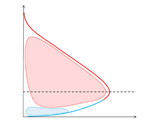
  ${U_+}$, ${\overline {u_+^{2}}}$ and ${(-\overline {uw})_+}$ plotted against ${z_+}$. These profiles are extracted at the S15 location ( $x/b=77$) from the complete set of 9000 PIV fields of WJ1 flow (case WJ1-6 in table 3). Vertical dotted lines in all plots mark the extent of the mesolayer $0.7\leq {\eta \sqrt {{Re_{\tau }}}}\leq 3$.

Figure 4. Profiles of (a)  ${U_+}$, (b) ${\overline {u_+^{2}}}$ and (c) ${(-\overline {uw})_+}$ plotted against ${z_+}$, at location S15 ( $x/b=77$) for flow WJ1. In this and all subsequent plots, the meso-overlap layer is the region between vertical dotted lines, and the region of counter-gradient momentum diffusion resides between vertical dashed lines. Note that the meso-overlap layer extent $0.7\leq {\eta \sqrt {{Re_{\tau }}}}\leq 3$ is marked according to the empirical limits found by Gupta et al. (Reference Gupta, Choudhary, Singh, Prabhakaran and Dixit2020).
Another peculiar feature of plane wall jets is evident from the profile of the Reynolds shear stress  ${(-\overline {uw})_+}$ shown in figure 4(c). Starting from positive values in the mesolayer region, the profile crosses the zero line at a wall-normal location which is marked by a dashed vertical line at ${z_+} \approx 220$. Another dashed vertical line around ${z_+} \approx 460$ marks the location ${z_{max}}$ where the mean velocity reaches the maximum value ${U_{max}}$. The region between these vertical dashed lines is characterized by $\partial U/\partial z>0$ and ${(-\overline {uw})} <0$ i.e. the wall-normal flux of streamwise mean momentum has a direction opposite to that of the gradient of mean velocity. This region is thus known as the region of ‘counter-gradient’ (momentum) diffusion and is a hallmark of plane wall-jet flows (Narasimha Reference Narasimha1990).
We shall frequently refer to the mesolayer and counter-gradient diffusion regions throughout the paper and mark their extents on various plots with dotted and dashed lines, respectively. We shall present PIV results (in this paper and Part 2) that shed important light on the dynamics and properties of these regions.
4. Spectral analysis
4.1. Hypothesis of wall and jet structural modes
We hypothesize that the structure of plane wall-jet flows consists of two distinct structural modes – the wall mode and the jet mode. The wall mode is expected to be characterized by motions that scale on the wall scales ( $\nu$ and ${U_{\tau }}$) akin to those in the near-wall region of TBLs, pipes and channels. The jet mode, on the other hand, is expected to feature motions that are governed by the jet scales ( ${z_{T}}$ and ${U_{max}}$). Gupta et al. (Reference Gupta, Choudhary, Singh, Prabhakaran and Dixit2020) have demonstrated that the mean velocity in wall jets indeed displays wall and jet scaling regimes that overlap in a region below the velocity maximum. This overlap, however, is not inertial but in fact a mesolayer that displays Reynolds-number dependence. The present hypothesis contends that this scaling of mean velocity is a manifestation of the underlying wall and jet structural modes. Although the idea of wall- and jet-scaled regions of the mean-velocity profile is not new to the literature on wall jets (Katz, Horev & Wygnanski Reference Katz, Horev and Wygnanski1992; Banyassady & Piomelli Reference Banyassady and Piomelli2015), explicit connection of these regions to structural components is largely missing except for a very few studies that are limited to a low and single Reynolds number (Banyassady & Piomelli Reference Banyassady and Piomelli2014; Gnanamanickam et al. Reference Gnanamanickam, Bhatt, Artham and Zhang2019). Our approach hypothesises that the turbulent eddies have these scaling behaviours which are reflected in the scaling of mean velocity. We aim to extensively investigate these structures from experiments over a range of Reynolds numbers. Further, we contend that the jet mode is a full free-jet mode with jet scaled motions residing in the inner as well as the outer regions of the flow; the wall mode resides only in the wall region. This proposal is unique compared with any other proposal in the literature.
4.2. Outline of the spectral analysis
Spectral analysis is a tool commonly used to examine the dominant energetic wavelengths that contribute to the energy and fluxes of turbulent motions (Balakumar & Adrian Reference Balakumar and Adrian2007). Further, such dominant wavelengths have been recognized as distinguishing spectral signatures of the structural modes such as very-large-scale motions in pipe flows (Balakumar & Adrian Reference Balakumar and Adrian2007) or superstructures in TBLs (Hutchins & Marusic Reference Hutchins and Marusic2007a; Monty et al. Reference Monty, Hutchins, Ng, Marusic and Chong2009). In the same spirit, we undertake spectral analysis of our HW and PIV data with the aim of uncovering the signatures (if any) of the wall and jet structural modes. To this end, we first present spectral energy maps of the  $u$ time series data from our HW measurements. This is followed by similar maps of the $u$ and $w$ spatial fields from our long-FOV PIV measurements. These give information about spectral contributions to ${\overline {u^{2}}}$ and ${\overline {w^{2}}}$. Next, we analyse the co-spectra of the $u$ and $w$ PIV fields to examine contributions of different wavelengths to the Reynolds shear stress ${(-\overline {uw})}$. The wall-normal gradients of these co-spectra yield the so-called force spectra that shed light on the spectral structure of ${\partial {(-\overline {uw})}/\partial z}$. We present these force spectra also. Since ${\partial {(-\overline {uw})}/\partial z}$ features in the mean streamwise momentum equation, the information from the co-spectra and force spectra reflects the dynamics. Further, multiplying the co-spectra of $u$ and $w$ by the mean-velocity gradient ${\partial U /\partial z}$ yields spectral structure of TKE production term ${{(-\overline {uw})}{\partial U /\partial z}}$, which is a dynamically important term in the TKE budget equation. In the present 2-D PIV measurements, the accessible part of the TKE is ${\overline {q^{2}}}$ where ${{\overline {q^{2}}}={\overline {u^{2}}}+{\overline {w^{2}}}}$. The TKE budget also involves turbulent transport term ${\partial {(-\overline {q^{2}w})}/\partial z}$ – wall-normal gradient of the triple product ${(-\overline {q^{2}w})}$. Since the focus of this study is to capture large-scale structures, our FOV extent is larger, which compromises the spatial resolution somewhat, precluding accurate estimation of the spatial derivatives of the instantaneous or fluctuating velocity fields. Therefore, the spectral analyses of quantities such as the fluctuating enstrophy, fluctuating velocity–vorticity products and TKE dissipation rate are not presented.
In the following, we shall examine spectral contributions to  ${\overline {u^{2}}}$, ${\overline {w^{2}}}$, ${(-\overline {uw})}$, ${\partial {(-\overline {uw})}/\partial z}$, ${(-\overline {q^{2}w})}$, ${{(-\overline {uw})}{\partial U /\partial z}}$ and ${\partial {(-\overline {q^{2}w})}/\partial z}$ in the wall-jet flow. For analysis of our long-FOV PIV data, direct computation of spatial spectra is used without invoking Taylor's hypothesis. For ${\overline {u^{2}}}$, we also present HW spectra where Taylor's hypothesis is used for converting frequencies to wavelengths. For each quantity, we shall present results in the sequence – (i) spectral maps, (ii) line spectra at salient wall-normal locations and (iii) wall-normal profiles of the total quantity and its scale-decomposed (large- and small-scale) contributions. We note that, in wall jets, spectra are not as well studied as for channels, pipes and TBLs. Moreover, for wall jets, we shall be plotting many quantities for the first time, such as co-spectra, force spectra, triple product spectra and transport spectra. Therefore, it is important to plot spectral maps first, in order to decide which salient wall-normal locations need to be chosen to plot the line spectra and what consensus wavelength should be used to spectrally decompose the statistics into large- and small-scale contributions. It is important to note that the streamwise location S15 ( $x/b=77$ in table 3) approximately marks the $x$-wise centre of our long FOV. Therefore, unless otherwise stated explicitly, we shall use the values of scales ( ${U_{\tau }}$, ${U_{max}}$, ${z_{T}}$, ${z_{max}}$ etc.) at the S15 location to normalize instantaneous, average and fluctuating values of various PIV fields.
4.3. Spectral contributions to  ${\overline {u^{2}}}$: HW data

4.3.1. The $u$ spectral maps: HW data

We first analyse the streamwise velocity fluctuation time series  $u(t)$ from HW measurements. We show the spectral analysis results for location S17 ( $x/b=92$) and compare them across all three Reynolds numbers (flows WJ1-8, WJ2-8 and WJ3-8 in table 3).
Figure 5 shows contours of the jet-scaled, pre-multiplied power spectral density (PSD) of  $u$, denoted by ${\varPhi _{uu}^{m}}$, plotted in the ${\lambda _{x}}$– $z$ plane, computed at the S17 location, for three flows WJ1, WJ2 and WJ3. Details of the computation of ${\varPhi _{uu}^{m}}$ may be found in Appendix C.1. Left and right vertical axes, respectively, plot wavelength in jet ( ${{\lambda _{x}}/{z_{T}}}$) and wall ( ${\lambda _{x}^+}={{\lambda _{x}} {U_{\tau }} /\nu }$) scalings whereas, the bottom and top horizontal axes, respectively, plot distance from the wall in jet ( $\eta =z/{z_{T}}$) and wall ( ${z_+}=z{U_{\tau }} / \nu$) scalings. Note that the horizontal extent of each plot is fixed in $\eta$ coordinates to enable comparison of the jet-mode features. It is clear that all flows have a strong outer energy site, marked by a cross $\times $ in figures 5(a)–5(c). This site is anchored at $\eta \approx 0.7$ and ${{\lambda _{x}}/{z_{T}}}\approx 5$ irrespective of Reynolds number, and thus corresponds to the jet mode of the structure of wall-jet flows. Note that significantly energetic wavelengths in this jet mode (at $\eta \approx 0.7$) range from $0.7{z_{T}}$ to $20{z_{T}}$ with the most energetic wavelength being $5{z_{T}}$. An inner energy site of wall-scaled motions, anchored at ${z_+}\approx 15$ and ${\lambda _{x}^+}\approx 1000$, is expected to be a universal feature of all wall-bounded flows, including TBLs (Mathis, Hutchins & Marusic Reference Mathis, Hutchins and Marusic2009), channels and pipes (Monty et al. Reference Monty, Hutchins, Ng, Marusic and Chong2009) and wall jets (Gnanamanickam et al. Reference Gnanamanickam, Bhatt, Artham and Zhang2019). This inner site is marked by a plus sign $+$ in figures 5(a)–5(c) and we shall associate it with the wall mode of the structure of wall jets. Figure 5 shows that the presence of the inner site is not very clear due to overwhelmingly strong outer site, but may still be discerned from the deflection of contours in the near-wall region (see also figure 11 of Gnanamanickam et al. Reference Gnanamanickam, Bhatt, Artham and Zhang2019).

Figure 5. Contours of jet-scaled pre-multiplied PSD  $\varPhi ^{m}_{uu}$ of the $u$ signal from HW data measured at the S17 location ( $x/b=92$) for flows (a) WJ1, (b) WJ2 and (c) WJ3. Contours are plotted on a plane with wall-normal distance on the horizontal axis and wavelength on the vertical axis. The extent of each plot is fixed in outer coordinates $\eta$ and $\lambda _x/z_T$. The meso-overlap layer $0.7\leq \eta \sqrt {{Re_{\tau }}}\leq 3$ proposed by Gupta et al. (Reference Gupta, Choudhary, Singh, Prabhakaran and Dixit2020) is marked by vertical dotted lines. Vertical dashed line shows location of velocity maximum. Wall or inner ( ${z_+}\approx 15$ and ${\lambda _{x}^+}\approx 1000$) and jet or outer ( $\eta \approx 0.7$ and ${{\lambda _{x}}/{z_{T}}}\approx 5$) energetic sites are marked, respectively, by black ‘ $+$’ and ‘ $\times$’ symbols. Horizontal dotted line at ${{\lambda _{x}}/{z_{T}}}=1$ marks the empirical cutoff used for scale decompositions.
The shape of the spectral map shows no dependence on Reynolds number. At low Reynolds number, the inner and outer sites appear spatially isolated, with the location of  ${U_{max}}$ (dashed line in figure 5a) acting as the demarcation between the two. Despite this, there is non-negligible energy present at ${z_+}\approx 15$ at long wavelengths $1\lessapprox {{\lambda _{x}}/{z_{T}}} \lessapprox 5$. All Reynolds numbers show significant influence of this long-wavelength jet mode in the regions of ${U_{max}}$, the mesolayer (region between vertical dotted lines) and all the way down up to the inner site location of ${z_+}\approx 15$ (figure 5b,c). Earlier studies in the literature (Launder & Rodi Reference Launder and Rodi1979, Reference Launder and Rodi1983; George et al. Reference George, Abrahamsson, Eriksson, Karlsson, Löfdahl and Wosnik2000; Barenblatt, Chorin & Prostokishin Reference Barenblatt, Chorin and Prostokishin2005; Gnanamanickam et al. Reference Gnanamanickam, Bhatt, Artham and Zhang2019) consider the part of the wall jet below ${U_{max}}$ to be akin to a regular TBL. If this were true, then the thickness of this TBL would be ${z_{max}}$ and the longest wavelengths associated with the superstructures ( ${\lambda _{x}^{ss}}$) in this TBL would be ${\lambda _{x}^{ss}}\approx 6{z_{max}}$ (Hutchins & Marusic Reference Hutchins and Marusic2007a; Monty et al. Reference Monty, Hutchins, Ng, Marusic and Chong2009). Since, ${z_{T}}/{z_{max}}\approx 6$ in our wall-jet experiments (see table 3), this longest wavelength turns out to be ${\lambda _{x}^{ss}}\approx {z_{T}}$. However, figure 5 provides evidence that significant energy, even at ${z_+} \approx 15$, resides in wavelengths much longer than ${z_{T}}$. Clearly, these long wavelengths may not be simply attributed to superstructures of the (supposed) TBL that extends from the wall up to ${z_{max}}$. Therefore, these long wavelengths ought to be associated with the presence of jet-mode motions even below ${z_{max}}$.
4.3.2. The $u$ line spectra: HW data

Spectral maps of figure 5 from § 4.3.1 suggest at least three salient wall-normal locations where line spectra may be plotted to get a quantitative estimate of the spectral energy content. These locations are the inner energy site ( ${z_+}\approx 15$), mesolayer ( ${z_+}\approx 1.8\sqrt {{Re_{\tau }}}$ approximate midpoint of the mesolayer) and outer energy site ( $\eta \approx 0.7$ or ${z_+}\approx 0.7{Re_{\tau }}$). Figure 6 shows line spectra of ${\varPhi _{uu}^{m}}$, taken out from the spectral maps of figure 5 and plotted at these wall-normal locations for all three Reynolds numbers. At the inner site (figure 6a), spectra show some Reynolds-number dependence, as expected, due to possible influence of viscous effects. For the remaining two locations (figure 6b,c), spectra collapse, indicating Reynolds-number similarity. At the inner site, the dominant wavelength seems to be ranging from ${\lambda _{x}}\approx {z_{T}}$ to $2.5{z_{T}}$, with lesser energy density at ${\lambda _{x}}\approx 5{z_{T}}$. As one moves out from the wall, a clear shift of the spectral peak to longer wavelengths is evident. In the mesolayer itself, the dominant wavelength ranges from $2.5{z_{T}}$ to $5{z_{T}}$, indicating jet-mode activity below ${z_{max}}$. In the outer layer, ${\lambda _{x}}\approx 5{z_{T}}$ becomes the most energetic wavelength at the outer energy site.

Figure 6. The HW line spectra  ${\varPhi _{uu}^{m}}$ plotted against the jet-scaled streamwise wavelength $\lambda /z_{T}$ at three different wall-normal locations; (a) inner site $z_+ \approx 15$, (b) midpoint of the mesolayer $z_+ \approx 1.8 \sqrt {{Re_{\tau }}}$ and (c) outer site $z_+\approx 0.7 {Re_{\tau }}$. Flows WJ1, WJ2 and WJ3 are shown. Vertical dotted, dashed-dotted and dashed lines, respectively, show streamwise wavelengths ${\lambda _{x}}={z_{T}}$, ${\lambda _{x}}=2.5{z_{T}}$ and ${\lambda _{x}}=5{z_{T}}$.
4.3.3. Profiles of total and scale-decomposed ${\overline {u^{2}}}$: HW data

Figure 5 also suggests an empirical demarcation between long- and short-wavelength motions to ascertain the relative contributions of these spectral ranges to the total variance  ${\overline {u^{2}}}$; such scale decompositions are common in TBL studies (Hutchins & Marusic Reference Hutchins and Marusic2007b; Mathis et al. Reference Mathis, Hutchins and Marusic2009; Smits, McKeon & Marusic Reference Smits, McKeon and Marusic2011; Ganapathisubramani et al. Reference Ganapathisubramani, Hutchins, Monty, Chung and Marusic2012). For wall jets, Gnanamanickam et al. (Reference Gnanamanickam, Bhatt, Artham and Zhang2019) have used ${\lambda _{x}}=2{z_{T}}$ as the cutoff wavelength for their HW experimental data at a single Reynolds number. Their choice is based on reasonable (yet empirical) separation between outer and inner sites with a cutoff wavelength sufficiently away from the inner site wavelength of ${\lambda _{x}^+}\approx 1000$. Our arguments in the preceding paragraph provide a heuristic basis for considering ${\lambda _{x}}={z_{T}}$ as an appropriate cutoff for scale decomposition in wall jets. Indeed, figure 5 shows that the ${\lambda _{x}}={z_{T}}$ cutoff (horizontal dotted line) separates the inner and outer sites reasonably well at all Reynolds numbers in our experiments. Therefore, we shall use ${\lambda _{x}}={z_{T}}$ as the cutoff for spectral decomposition of all statistics. It may be noted that this cutoff decomposes a statistic into contributions from long jet-mode wavelengths ( ${\lambda _{x}}\geq {z_{T}}$) and contributions from shorter wavelengths ( ${\lambda _{x}}<{z_{T}}$) comprising the wall mode and as well as the residual shorter wavelengths from the jet mode. The procedure adopted for spectral decomposition of HW data is outlined in Appendix C.1.
Figure 7(a) shows the viscous-scaled profiles of total  ${\overline {u^{2}}}$ (solid lines) and its long-wavelength component (dashed lines) for the HW data of figure 5 at all Reynolds numbers; here, ${\overline {u_+^{2}}}={\overline {u^{2}}}/{U_{\tau }}^2$ and ${z_+}=z{U_{\tau }}/\nu$. Shaded vertical bands indicate the range of upper and lower limits of the mesolayer over the range of Reynolds numbers studied here. Profiles of total ${\overline {u_+^{2}}}$ collapse below ${z_+}=15$ but not anywhere else. Profiles of the long-wavelength contribution do not show any collapse; in fact, the profiles cross-over at ${z_+}=15$ with opposite Reynolds-number trends on its either side. The near-wall peak of total ${\overline {u_+^{2}}}$, although not clearly discernible due to the large outer peak, remains located around ${z_+}=15$ (dashed-dotted vertical line) and its magnitude appears to scale for the two larger Reynolds numbers. This is interesting because the HW spatial resolution deteriorates from ${l_+}=21$(WJ1-8) to $40$(WJ3-8), as seen in table 1, which suggests that the peak value should reduce. Therefore, there appears to be a Reynolds-number-dependent increasing contribution that counterbalances the ${l_+}$ effect. This contribution comes from the short-wavelength component (dashed-dotted lines) as seen in figure 7(b). Below ${z_+}=15$, the long- and short-wavelength contributions have opposite Reynolds-number trends so that the total ${\overline {u_+^{2}}}$ profiles show collapse in that region.

Figure 7. Scale decomposition of  ${\overline {u^{2}}}$ profiles from HW data at location S17 (see table 1) for flows WJ1-8, WJ2-8 and WJ3-8. Solid lines in each plot show profiles of the total value of ${\overline {u^{2}}}$. Panels (a,b) respectively show long- and short-wavelength contributions to total ${\overline {u^{2}}}$ in viscous scaling i.e. ${\overline {u_+^{2}}}$ vs ${z_+}$. Panels (c,d) respectively show long- and short-wavelength contributions to total ${\overline {u^{2}}}$ in jet scaling i.e. ${\overline {u_{m}^2}}$ vs $\eta$. Dashed-dotted vertical line shows wall-normal locations ${z_+}=15$ in panels (a,b), and $\eta =0.7$ in panels (c,d). In each plot, the left (right) shaded vertical band indicates the range of lower (upper) limits of the mesolayer over the present range of Reynolds numbers.
Figures 7(c) and 7(d) show the same set of profiles as in figures 7(a) and 7(b), respectively, but now plotted in the outer or jet scaling; here,  ${\overline {u_{m}^2}}={\overline {u^{2}}}/{U_{max}}^2$ and $\eta ={z/z_{T}}$. For the two higher Reynolds numbers, the profiles of total ${\overline {u_{m}^2}}$ and the long-wavelength contribution to it, scale very well from within the mesolayer all the way across the entire outer layer (figure 7c). The same is true for the short-wavelength contribution (figure 7d). The outer peak value and location ( $\eta =0.7$) in both cases scale on the jet variables. This demonstrates Reynolds-number similarity of energetic motions (with respect to jet scaling) at these Reynolds numbers. The lowest Reynold-number data appears to display a low-Reynolds-number effect which is consistently observed in these as well as subsequent plots of PIV analysis.
4.4. Spectral contributions to ${\overline {u^{2}}}$: PIV data

4.4.1. The $u$ spectral maps: PIV data

Figure 8 plots contours of the jet-scaled, pre-multiplied PSD of  $u$, denoted by ${\varPhi _{uu}^{m}}$, plotted in the ${\lambda _{x}}$– $z$ plane for all three Reynolds numbers WJ1, WJ2 and WJ3. These are maps of direct spatial spectra computed from the long-FOV PIV data without making use of Taylor's hypothesis of frozen turbulence. Details of the computation of ${\varPhi _{uu}^{m}}$ may be found in Appendix C.2. The extents of the mesolayer (vertical dotted lines) and counter-gradient diffusion region (vertical dashed lines), corresponding to the S15 location, are also marked. Contour colour scale and levels are same for all plots so that fair comparison is possible; contour levels help to elucidate Reynolds-number effects. The location of the inner energy site is marked only for reference since the present PIV measurements do not extend close enough to the wall to capture the inner site. The streamwise extent $L_x\approx 5.2{z_{T}}$ ( ${z_{T}}$ for S15 location) of the long FOV of PIV is sufficient to capture the outer site peak seen at ${\lambda _{x}}\approx 5{z_{T}}$ in the HW spectra (figure 5); wavelengths longer than $5.2{z_{T}}$ are, however, not captured.

Figure 8. Contours of jet-scaled pre-multiplied PSD  $\varPhi ^{m}_{uu}$ of $u$ signal from spatial 2-D PIV data for flows (a) WJ1, (b) WJ2 and (c) WJ3. Contours are plotted on a plane with wall-normal distance on the horizontal axis and wavelength on the vertical axis. The extent of each plot is fixed in outer coordinates $\eta$ and $\lambda _x/z_T$. The meso-overlap layer $0.7\leq \eta \sqrt {{Re_{\tau }}}\leq 3$ proposed by Gupta et al. (Reference Gupta, Choudhary, Singh, Prabhakaran and Dixit2020) is marked by vertical dotted lines; these limits correspond to location S15 ( $x/b=77$). Vertical dashed lines mark the limits of the counter-gradient momentum diffusion region corresponding to location S15 ( $x/b=77$). Horizontal dotted line at ${{\lambda _{x}}/{z_{T}}}=1$ marks the empirical cutoff used for scale decompositions. Similar to figure 5, wall or inner ( ${z_+}\approx 15$ and ${\lambda _{x}^+}\approx 1000$) and jet or outer ( $\eta \approx 0.7$ and ${{\lambda _{x}}/{z_{T}}}\approx 5$) energetic sites are marked, respectively, by black ‘ $+$’ and ‘ $\times$’ symbols.
Figure 8 shows that the shape of PIV spatial spectral maps shows no dependence on Reynolds number, which is consistent with the HW spectral maps of figure 5. The outer site located at  ${\lambda _{x}}\approx 5{z_{T}}$ is well captured and is marked by a $+$ sign. Note that the spectral resolution is somewhat coarse at longer wavelengths; the first three long wavelengths are $5.2{z_{T}}$, $2.5{z_{T}}$ and $1.7{z_{T}}$. On the whole, the PIV spatial spectral maps of figure 8 are in excellent agreement with the HW spectral maps of figure 5. Specifically, we observe that the wall-ward expanse of the outer site broadens with Reynolds number and the PSD of long wavelengths progressively increases in the counter-gradient and mesolayer regions i.e. the jet mode grows stronger in the region below ${z_{max}}$. This is evident from the fact that contour levels in the inner and outer regions (corresponding to reddish–yellow colour) are well separated for flow WJ1, but expand and merge across the velocity maximum for flows WJ2 and WJ3. It is interesting to note that, although the band of long wavelengths carrying significant energy in these regions is $1\leq {{\lambda _{x}}/{z_{T}}} \leq 5$, the most energetic wavelength appears to be ${\approx }2.5{z_{T}}$. This indicates that, while the outer site is dominated by $5{z_{T}}$ motions, the influence of the jet mode in the regions below ${z_{max}}$ features dominance of $2.5{z_{T}}$ motions. Also, the scale-separation cutoff ${\lambda _{x}}={z_{T}}$, shown by a dotted horizontal line in each plot of figure 8, appears to be reasonable in separating inner and outer energy sites.
4.4.2. The $u$ line spectra: PIV data

Spectral maps of figure 8 from § 4.4.1 suggest three salient wall-normal locations for which line spectra may be plotted for a quantitative estimate of the spectral energy content. These locations are the mesolayer ( ${z_+}\approx 1.8\sqrt {{Re_{\tau }}}$ approximate midpoint of the mesolayer), the counter-gradient region ( ${z_+}\approx 0.12{Re_{\tau }}$ is within the counter-gradient region for the range of Reynolds number studied here) and the outer energy site ( $\eta \approx 0.7$ or ${z_+}\approx 0.7{Re_{\tau }}$). Figure 9 shows line spectra of ${\varPhi _{uu}^{m}}$, taken from the spectral maps of figure 8 and plotted at these wall-normal locations for all three Reynolds numbers. For all locations in figure 8, spectra for the two larger Reynolds numbers collapse, indicating Reynolds-number similarity consistent with figures 5(b) and 5(c). In the mesolayer, the dominant wavelength is ${\lambda _{x}}=2.5{z_{T}}$ (figure 8a and figure 5b). In the counter-gradient region, ${\lambda _{x}}=2.5{z_{T}}$ and $5{z_{T}}$ both become equally energetic, whereas at the outer site ${\lambda _{x}}=5{z_{T}}$ dominates the spectrum. Also, note that, from the counter-gradient region to the outer site, the most dramatic increase in PSD values occurs for long-wavelength jet-mode motions ${\lambda _{x}}\geq {z_{T}}$.

Figure 9. The PIV line spectra  ${\varPhi _{uu}^{m}}$ plotted against the jet-scaled streamwise wavelength ${\lambda _{x}}/{z_{T}}$ at three different wall-normal locations; (a) midpoint of mesolayer $z_+ \approx 1.8 \sqrt {{Re_{\tau }}}$, (b) counter-gradient region $z_+ \approx 0.12 {Re_{\tau }}$ and (c) outer site $z_+\approx 0.7 {Re_{\tau }}$. Flows WJ1, WJ2 and WJ3 are shown. Vertical dotted, dashed-dotted and dashed lines, respectively, show streamwise wavelengths ${\lambda _{x}}={z_{T}}$, ${\lambda _{x}}=2.5{z_{T}}$ and ${\lambda _{x}}=5{z_{T}}$.
4.4.3. Profiles of total and scale-decomposed ${\overline {u^{2}}}$: PIV data

Figure 10 shows the profiles of  ${\overline {u_{m}^2}}={\overline {u^{2}}}/{U_{max}}^2$ and their scale decomposition, plotted against $\eta ={z/z_{T}}$. Details of the scale decomposition calculations are given in Appendix C.2. Since profiles from all Reynolds numbers are shown, the extents of the mesolayer and counter-gradient diffusion region (measured at the S15 location) for each flow are different. As such, in this as well as all subsequent plots of scale-decomposed profiles, shaded areas are used to denote the range of wall-normal locations that covers the beginning and end of these regions over the present range of Reynolds numbers. The plot shows that all three groups of curves, namely total, ${\lambda _{x}}\geq {z_{T}}$ and ${\lambda _{x}}<{z_{T}}$, scale well (except very near the wall) for the two higher- $Re$ flows WJ2 and WJ3 displaying Reynolds-number similarity. The low- $Re$ case WJ1 shows a lack of scaling, implying a low- $Re$ effect present in the data. Moreover, this low- $Re$ effect is severe for ${\lambda _{x}}\geq {z_{T}}$ motions, with ${\lambda _{x}}<{z_{T}}$ motions virtually unaffected. That is, the low- $Re$ effect in the total curves is almost entirely contributed by ${\lambda _{x}}\geq {z_{T}}$ motions. Within each group, the curves fan out very close to the wall, indicating the increasing importance of viscous scaling in the mesolayer. For ${\overline {u_{m}^2}}$ in WJ2 and WJ3 (figure 10a), ${\lambda _{x}}\geq {z_{T}}$ motions contribute $79\,\%$ and $64\,\%$ of the total variance, respectively, at the outer peak and in the mesolayer. The corresponding values for ${\lambda _{x}}<{z_{T}}$ motions are $21\,\%$ and $36\,\%$, respectively. Note that the ${\lambda _{x}}\geq {z_{T}}$ contributions are always larger than the ${\lambda _{x}}<{z_{T}}$ contributions, with the latter showing practically no variation in the wall-normal direction.

Figure 10. Total and scale-decomposed profiles of  ${\overline {u_{m}^2}}$ from PIV data plotted against the jet-scaled wall-normal distance $\eta$. Plot shows comparison of flows WJ1, WJ2 and WJ3. Cutoff wavelength used is ${\lambda _{x}}={z_{T}}$. Shaded vertical bands denote the range of wall-normal locations that covers the beginning and end of the mesolayer (bands between dotted lines) and the counter-gradient region (bands between dashed lines) over the present range of Reynolds numbers.
4.5. Spectral contributions to ${\overline {w^{2}}}$: PIV data

4.5.1. The $w$ spectral maps: PIV data

Figure 11 plots contours of the jet-scaled, pre-multiplied PSD of  $w$, denoted by ${\varPhi _{ww}^{m}}$, plotted in a fashion similar to the contours of ${\varPhi _{uu}^{m}}$ of figure 8. Details of the computation of ${\varPhi _{ww}^{m}}$ may be found in Appendix C.2. Spectra of figure 11 show interesting features. First, as in the case of $u$ spectra, the shape of the $w$ spectra also shows no dependence on Reynolds number. Secondly, the shape of the $w$ spectra is clearly different from that of $u$ spectra; the inner site is completely absent in ${\varPhi _{ww}^{m}}$. This is due to impermeability constraint or blocking effect of the wall which strongly influences $w$ fluctuations. Third, a clear outer site (marked by a circle) for energy of $w$ fluctuations is located at $\eta \approx 0.7$ and ${{\lambda _{x}}/{z_{T}}}\approx 2.5$. Note that, the wall-normal locations of the outer sites of $u$ and $w$ are identical ( $\eta \approx 0.7$) but their wavelengths are clearly different, ${\lambda _{x}}\approx 5{z_{T}}$ for the $u$ spectra and ${\lambda _{x}}\approx 2.5{z_{T}}$ for the $w$ spectra. Thus, one may conclude that the (structural) jet mode comprises at least two dominant, distinct, energetic submodes viz. submode 1 ( ${\lambda _{x}}\approx 5{z_{T}}$) and submode 2 ( ${\lambda _{x}}\approx 2.5{z_{T}}$). The scale-separation cutoff ${\lambda _{x}}={z_{T}}$ does not seem to have a major role here since the inner site for $w$ is non-existent.

Figure 11. Contours of jet-scaled pre-multiplied PSD  $\varPhi ^{m}_{ww}$ of $w$ signal from spatial 2-D PIV data for flows (a) WJ1, (b) WJ2 and (c) WJ3. Contours are plotted on a plane with wall-normal distance on the horizontal axis and wavelength on the vertical axis. The extent of each plot is fixed in outer coordinates $\eta$ and ${{\lambda _{x}}/{z_{T}}}$. The meso-overlap layer $0.7\leq \eta \sqrt {{Re_{\tau }}}\leq 3$ proposed by Gupta et al. (Reference Gupta, Choudhary, Singh, Prabhakaran and Dixit2020) is marked by vertical dotted lines; these limits correspond to location S15 ( $x/b=77$). Vertical dashed lines mark the limits of the counter-gradient momentum diffusion region corresponding to location S15 ( $x/b=77$). Horizontal dotted line at ${{\lambda _{x}}/{z_{T}}}=1$ marks the empirical cutoff used for scale decompositions. The jet or outer energetic site for $w$ fluctuations is located at $\eta \approx 0.7$ and ${{\lambda _{x}}/{z_{T}}}\approx 2.5$, and is marked by a black circle; there is no wall or inner site for $w$ fluctuations. Energy sites for $u$ fluctuation ( $+$ and $\times$) are also shown reference.
4.5.2. The $w$ line spectra: PIV data

Since the spectral contours of figure 11 from § 4.5.1 do not suggest any specific locations other than the outer energy site, line spectra of  $w$ fluctuation are plotted in figure 12 at the same three wall-normal locations that are used in figure 9 for the line spectra of $u$ fluctuation. Figure 12 shows that the $w$ spectra show Reynolds-number similarity for the two higher Reynolds numbers only at the outer site (panel c) but not in the mesolayer and counter-gradient regions (panels a,b, respectively). In fact, except for a small portion at shorter wavelengths, the spectral density is seen to decrease with Reynolds number in the mesolayer and increase in the counter-gradient region. This is to be contrasted with the Reynolds-number-similar behaviour of the $u$ spectra at all heights (figure 9). Further, while long wavelengths are almost absent in the mesolayer (panel a), a clear and progressive shift to longer wavelengths (panels b,c) is evident and a spectral peak of submode 2 ( ${\lambda _{x}}=2.5{z_{T}}$) emerges at the outer site (panel c).

Figure 12. The PIV line spectra  ${\varPhi _{ww}^{m}}$ plotted against the jet-scaled streamwise wavelength ${\lambda _{x}}/{z_{T}}$ at three different wall-normal locations; (a) midpoint of mesolayer ${z_+} \approx 1.8 \sqrt {{Re_{\tau }}}$, (b) counter-gradient region ${z_+} \approx 0.12 {Re_{\tau }}$ and (c) outer site ${z_+}\approx 0.7 {Re_{\tau }}$. Flows WJ1, WJ2 and WJ3 are shown. Vertical dotted, dashed-dotted and dashed lines, respectively, show streamwise wavelengths ${\lambda _{x}}={z_{T}}$, ${\lambda _{x}}=2.5{z_{T}}$ and ${\lambda _{x}}=5{z_{T}}$.
4.5.3. Profiles of total and scale-decomposed ${\overline {w^{2}}}$: PIV data

Figure 13 plots the profiles of total and scale-decomposed  ${\overline {w_{m}^2}}={\overline {w^{2}}}/{U_{max}}^2$ against $\eta ={z/z_{T}}$. Details of the scale decomposition calculations may be found in Appendix C.2. Similar to figure 10, shaded areas are used to denote the range of wall-normal locations that covers the beginning and end of the mesolayer and counter-gradient regions over the present range of Reynolds numbers. It may be seen that all three groups of curves, namely total, ${\lambda _{x}}\geq {z_{T}}$ and ${\lambda _{x}}<{z_{T}}$, scale quite well throughout (even in the mesolayer, implying lack of a viscous influence on $w$ fluctuation) for the two higher- $Re$ flows WJ2 and WJ3 displaying Reynolds-number similarity; WJ1 suffers from low- $Re$ effects. This low- $Re$ effect in ${\overline {w_{m}^2}}$ is observed to be equally severe for ${\lambda _{x}}\geq {z_{T}}$ motions and ${\lambda _{x}}<{z_{T}}$ motions; for ${\overline {u_{m}^2}}$ it is severe only for ${\lambda _{x}}\geq {z_{T}}$ motions (figure 10). Thus, for ${\overline {w_{m}^2}}$, the low- $Re$ effect in the total curves is contributed by both types of scale-decomposed motions (figure 13). As to the relative contributions to the total ${\overline {w_{m}^2}}$, figure 13 shows that, at the outer peak, $58\,\%$ of the total variance is contributed by ${\lambda _{x}}\geq {z_{T}}$ and $42\,\%$ by ${\lambda _{x}}<{z_{T}}$ motions i.e. both spectral ranges contribute significantly there. Interestingly, as one moves closer to the wall from the outer region, scale-decomposed curves cross each other around $\eta \approx 0.4$ with ${\lambda _{x}}\geq {z_{T}}$ contributions rapidly going to smaller values than the ${\lambda _{x}}<{z_{T}}$ contributions below this location (figure 13). At the wall-ward end of the mesolayer, virtually all ${\overline {w_{m}^2}}$ is contributed by ${\lambda _{x}}<{z_{T}}$ motions. This is consistent with the blocking effect or the impermeability boundary condition imposed by the solid wall, which does not allow large-scale motions to produce wall-normal velocities of the same order as the wall-parallel velocities. These observations also highlight the highly unisotropic character of near-wall turbulence in wall jets.

Figure 13. Total and scale-decomposed profiles of  ${\overline {w_{m}^2}}$ plotted against the jet-scaled wall-normal distance $\eta$. Plot shows comparison of flows WJ1, WJ2 and WJ3. Cutoff wavelength used is ${\lambda _{x}}={z_{T}}$. Shaded vertical bands denote the range of wall-normal locations that covers the beginning and end of the mesolayer (bands between dotted lines) and counter-gradient region (bands between dashed lines) over the present range of Reynolds numbers.
4.6. Spectral contributions to ${(-\overline {uw})}$: PIV data

4.6.1. The $-u$ and $w$ co-spectral maps: PIV data


The use of co-spectra is quite common in the study of atmospheric flows (Stull Reference Stull1988) but not so common in laboratory flows until recently. In pipe flows, Guala, Hommema & Adrian (Reference Guala, Hommema and Adrian2006) have found that the co-spectra and force spectra of  $-u$ and $w$ in the near-wall region receive significant contributions from the large- and very-large-scale motions; their study has used HW anemometry for turbulence measurements. Balakumar & Adrian (Reference Balakumar and Adrian2007) have extended this work to channel flows and zero-pressure-gradient TBLs. Recently, Chin et al. (Reference Chin, Philip, Klewicki, Ooi and Marusic2014) have investigated force spectra in pipe-flow DNS data in terms of velocity–vorticity correlations. The present work stands out compared with these earlier laboratory studies in two respects. First, we report co-spectra and force spectra of $-u$ and $w$ from PIV measurements; we are not aware of any prior work that reports these spectra using PIV measurements. Secondly, the behaviour of the co-spectra and force spectra of $-u$ and $w$ in wall jets has never been reported so far in the literature. Our study therefore makes these two important contributions.
Figure 14 plots the contours of jet-scaled, premultiplied, power co-spectral density (PCSD)  ${\varPhi _{(-uw)}^{m}}$ of the $-u$ and $w$ fluctuations constructed from PIV data for flows WJ1, WJ2 and WJ3. Details of the procedure for computing ${\varPhi _{(-uw)}^{m}}$ from spatial PIV data are given in Appendix C.3. Several new interesting features may be observed. First, we consider the outer part of the flow beyond the velocity maximum i.e. $\eta >0.15$. Here, the PCSD values are negative so that ${(-\overline {uw})}<0$, which is consistent with diffusion of mean momentum down the mean-velocity gradient in this region of ${\partial U /\partial z}<0$. A strong outer site for PCSD is observed at $\eta \approx 0.7$ and ${{\lambda _{x}}/{z_{T}}}\approx 5$ (marked by a $\times$). This site matches well with the corresponding outer site for the PSD of $u$ fluctuation (figure 8). At any height $\eta >0.15$, the PCSD is unimodal, with wavelengths carrying significant Reynolds shear stress in the range $0.1\leq {{\lambda _{x}}/{z_{T}}}\leq 5$ irrespective of Reynolds number (upper limit is fixed due the FOV constraint). This indicates that the contribution to ${(-\overline {uw})}$ in this region of the flow comes purely from the jet-mode wavelengths that scale on ${z_{T}}$. Next, we consider the mesolayer marked as the near-wall region between vertical dotted lines. In the mesolayer, PCSD values are positive so that ${(-\overline {uw})}>0$, which is consistent with diffusion of mean momentum down the mean-velocity gradient in this region of ${\partial U /\partial z}>0$. Towards the wall end of the mesolayer, the PCSD curves appear unimodal with a broad plateau-like region around ${\lambda _{x}}\approx 0.7{z_{T}}$. Also, the wavelengths carrying significant Reynolds shear stress here range from ${\lambda _{x}^+}\geq 100$ to ${{\lambda _{x}}/{z_{T}}}\leq 5$ at all Reynolds numbers. This indicates that both wall and jet modes produce significant Reynolds shear stress in this region. It is known that the wall mode is located at ${z_+}\approx 30$ and ${\lambda _{x}^+}\approx 700$ in channel flows (see figure 8 from Chin et al. Reference Chin, Philip, Klewicki, Ooi and Marusic2014). Assuming that the wall mode is universal, its location is marked in figure 14 with a five-pointed star. As one moves away from the wall, this bimodal character of the PCSD becomes readily evident at the outer edge of the mesolayer. At this height, a clear separation between wall and jet modes may be seen with ${{\lambda _{x}}/{z_{T}}}\approx 1$ as a reasonable demarcation between the two. The wall mode is seen to peak around ${\lambda _{x}^+}\approx 500$ while the jet mode peaks at ${{\lambda _{x}}/{z_{T}}}\approx 2.5$ (submode 2). Gupta et al. (Reference Gupta, Choudhary, Singh, Prabhakaran and Dixit2020) have envisioned the mean-velocity scaling in wall jets to consist of wall and jet scaling regions that overlap in the mesolayer, which retains a Reynolds-number dependence. Results of figure 14 emphatically confirm that the dynamical aspects also follow this structure, with the wall and jet structural modes overlapping in the mesolayer.

Figure 14. Contours of jet-scaled pre-multiplied PCSD  $\varPhi ^{m}_{(-uw)}$ of $u$ and $w$ signals from spatial 2-D PIV data for flows (a) WJ1, (b) WJ2 and (c) WJ3. Contours are plotted on a plane with wall-normal distance on the horizontal axis and wavelength on the vertical axis. The extent of each plot is fixed in outer coordinates $\eta$ and ${{\lambda _{x}}/{z_{T}}}$. The meso-overlap layer $0.7\leq \eta \sqrt {{Re_{\tau }}}\leq 3$ proposed by Gupta et al. (Reference Gupta, Choudhary, Singh, Prabhakaran and Dixit2020) is marked by vertical dotted lines; these limits correspond to location S15 ( $x/b=77$). Vertical dashed lines mark the limits of the counter-gradient momentum diffusion region corresponding to location S15 ( $x/b=77$). Horizontal dotted line at ${{\lambda _{x}}/{z_{T}}}=1$ marks the empirical cutoff used for scale decompositions. Horizontal dashed dotted line marks submode 2 of the jet mode. The wall or inner site for the co-spectra of $u$ and $w$ is shown by a five-pointed star at ${z_+}\approx 30$ and ${\lambda _{x}^+}\approx 700$. The jet or outer energy site for $u$ fluctuation is also shown for reference, which coincides well with the location of the outer co-spectral peak.
Results presented until now indicate that the jet-mode activity apparently resides on both sides of the velocity maximum. Therefore, it might be apt to classify it as the inner and outer parts of the jet mode (inner jet mode and outer jet mode for brevity). As one moves out further from the mesolayer into the counter-gradient diffusion region (region between vertical dashed lines), it is seen that a large negative contribution is received from the outer jet mode ( ${{\lambda _{x}}/{z_{T}}}\geq 0.3$) whereas the positive contribution from the wall mode remains rather limited. The spectral character changes from bimodal in the mesolayer to weakly trimodal in the counter-gradient region. For all Reynolds numbers, contours of negative PCSD appear to cross the velocity maximum ( $\eta \approx 0.15$) line at ${{\lambda _{x}}/{z_{T}}}\approx 0.3$ (scaling on ${z_{T}}$) demonstrating intrusion of the outer jet mode into the counter-gradient diffusion region, consistent with the suggestions in the earlier wall-jet studies (Gnanamanickam et al. Reference Gnanamanickam, Bhatt, Artham and Zhang2019; Bhatt & Gnanamanickam Reference Bhatt and Gnanamanickam2020). Moreover, within this region, the dominant wavelengths of the outer jet mode are ${{\lambda _{x}}/{z_{T}}}\approx 1$ and ${{\lambda _{x}}/{z_{T}}}\approx 5$ (submode 1). In fact, the bimodality of the mesolayer PCSD ( ${\lambda _{x}^+}\approx 500$ and ${{\lambda _{x}}/{z_{T}}}\approx 2.5$ or submode 2 of the inner jet mode) seems to split the outer jet mode in the counter-gradient region into two dominant wavelengths ${{\lambda _{x}}/{z_{T}}}\approx 1$ and ${{\lambda _{x}}/{z_{T}}}\approx 5$ (submode 1). These observations, for the first time, lend strong quantitative support to the influence of ‘long arm of the jet’ in the counter-gradient region of wall jets anticipated by Narasimha (Reference Narasimha1990).
Finally, if one focuses on jet-mode wavelengths  ${{\lambda _{x}}/{z_{T}}}\geq 1$ in the contour map, then the structure of the jet mode is a dipole extending across the height of the flow. This dipole has positive PCSD values in the near-wall (inner jet mode) region up to the beginning of the counter-gradient region and negative values from the counter-gradient region all the way into the outer region (outer jet mode). This dipole structure is typical of free jets (Deo, Mi & Nathan Reference Deo, Mi and Nathan2008) but in the case of wall jets, the pole in the near-wall region appears to be somewhat crammed and sandwiched between the wall and the beginning of counter-gradient region. With increasing Reynolds number, the outer jet mode appears to encroach deeper down below the velocity maximum, consistent with what has been suggested in the literature Gnanamanickam et al. (Reference Gnanamanickam, Bhatt, Artham and Zhang2019) and Bhatt & Gnanamanickam (Reference Bhatt and Gnanamanickam2020). This suggests that the asymptotic state of a wall jet in the limit of infinite Reynolds number may well be a half-free jet, as proposed by Gersten (Reference Gersten2015). However, more data at higher Reynolds numbers are needed to confirm this trend conclusively.
4.6.2. The $-u$ and $w$ line co-spectra: PIV data


Co-spectral contours of figure 14 from § 4.6.1 suggest specific locations where line co-spectra may be plotted to gain quantitative information about the spectral density of wall and jet-mode motions that contribute to the wall-normal turbulent flux of streamwise mean momentum. Figure 15 shows these line spectra. It may be observed that, at the outer end of the mesolayer (panel a), line spectra show clear bimodal character with equally strong, positive wall mode ( ${\lambda _{x}^+}\approx 500$) and inner jet mode (submode 2, ${\lambda _{x}}=2.5{z_{T}}$) spectral peaks. Both modes transport momentum down the mean velocity gradient. As one moves out into the counter-gradient region (panel b), the character changes to weakly trimodal; the positive wall-mode is vanishing to very low values (gradient transport) and negative outer jet mode seems to be splitting into ${\lambda _{x}}={z_{T}}$ and ${\lambda _{x}}=5{z_{T}}$ (counter-gradient transport). This splitting is due to the positive inner jet mode (gradient transport) located at ${\lambda _{x}}=2.5{z_{T}}$ as seen in contour plots of figure 14. Finally, at the outer site (panel c), only negative outer jet mode (gradient transport) persists.

Figure 15. The PIV line co-spectra  ${\varPhi _{(-uw)}^{m}}$ plotted against the jet-scaled streamwise wavelength ${\lambda _{x}}/{z_{T}}$ at three different wall-normal locations; (a) outer end of the mesolayer ${z_+} \approx 3 \sqrt {{Re_{\tau }}}$, (b) counter-gradient region ${z_+} \approx 0.12 {Re_{\tau }}$ and (c) outer site ${z_+}\approx 0.7 {Re_{\tau }}$. Flows WJ1, WJ2 and WJ3 are shown. Vertical dotted, dashed-dotted and dashed lines, respectively, show streamwise wavelengths ${\lambda _{x}}={z_{T}}$, ${\lambda _{x}}=2.5{z_{T}}$ and ${\lambda _{x}}=5{z_{T}}$.
4.6.3. Profiles of total and scale-decomposed ${(-\overline {uw})}$: PIV data

Figure 16 shows the total and scale-decomposed profiles of  ${(-\overline {uw})_m}={(-\overline {uw})}/{U_{max}}^2$ plotted against $\eta$ (see Appendix C.3 for scale decomposition procedure). The low- $Re$ effect in flow WJ1 and Reynolds-number similarity of flows WJ2 and WJ3 discussed before are evident in this plot too. For ${(-\overline {uw})_m}$ in WJ2 and WJ3 (figure 16), ${\lambda _{x}}\geq {z_{T}}$ contributions amount to ${\approx }84\,\%$ and ${\approx }33\,\%$ of the total momentum flux, respectively, at the outer peak and in the mesolayer (see zoomed inset in the plot). The corresponding contributions from ${\lambda _{x}}<{z_{T}}$ motions are ${\approx }16\,\%$ and ${\approx }66\,\%$, respectively. Thus, the ${\lambda _{x}}\geq {z_{T}}$ contribution to the mesolayer momentum flux is not negligible. This may seem counter-intuitive in view of the results of figure 13, where the ${\lambda _{x}}\geq {z_{T}}$ contributions to ${\overline {w_{m}^2}}$ go to zero rapidly in the mesolayer as the wall is approached. However, the large-scale ${\lambda _{x}}\geq {z_{T}}$ motions could amplitude modulate the near-wall $w$ signals, generating a significant fraction of the large-scale momentum flux which would otherwise be absent in the case of a linear superposition of scales without a nonlinear interaction. Although a detailed account of amplitude modulation in our wall-jet experiments is out of the scope of this work, this could potentially explain the generation of $33\,\%$ of the total momentum flux in the mesolayer by the large-scale ${\lambda _{x}}\geq {z_{T}}$ motions. It may further be noted that both the scale-decomposed contributions ( ${\lambda _{x}}\geq {z_{T}}$ and ${\lambda _{x}}<{z_{T}}$) are positive in the mesolayer and negative in the outer layer, with the changeover taking place somewhere close to the wall-ward end of the counter-gradient region. It is interesting that most of the counter-gradient momentum flux is contributed by ${\lambda _{x}}\geq {z_{T}}$ motions with very little contribution coming from ${\lambda _{x}}<{z_{T}}$ motions. This clearly supports the present finding that the outer jet mode plays a crucial role in reversing the gradient transport of momentum in the region below the velocity maximum.

Figure 16. Total and scale-decomposed profiles of  ${(-\overline {uw})_m}$ plotted against the jet-scaled wall-normal distance $\eta$. Each plot shows comparison of flows WJ1, WJ2 and WJ3. The cutoff wavelength used is ${\lambda _{x}}={z_{T}}$. Inset in plot shows zoomed view of the mesolayer region. Shaded vertical bands denote the range of wall-normal locations that covers the beginning and end of the mesolayer (bands between dotted lines) and counter-gradient region (bands between dashed lines) over the present range of Reynolds numbers.
4.7. Spectral contributions to turbulent shear force ${\partial {(-\overline {uw})}/\partial z}$: PIV data

4.7.1. Force spectral maps: PIV data
Wall-normal gradient of the PCSD of  $-u$ and $w$ highlights spectral contributions to ${\partial {(-\overline {uw})}/\partial z}$ at various heights from the wall. Thus, ${\partial \varPhi _{(-uw)}^{m}/\partial \eta }$ represents the so-called force spectrum (Chin et al. Reference Chin, Philip, Klewicki, Ooi and Marusic2014) or turbulent shear force PSD, and is plotted in figure 17 in the form of a contour map; note that the wall-normal gradient is with respect to the jet or outer coordinate $\eta$. Further, it may be noted that ${\partial \varPhi _{(-uw)}^{m}/\partial \eta }$ must satisfy ${\partial {(-\overline {uw})_m} /\partial \eta }=\int _{0}^{\infty }[{\partial \varPhi _{(-uw)}^{m}/\partial \eta }]\,\textrm {d}(\ln {k_{x}})$. Similar to Chin et al., contours of ${\partial \varPhi _{(-uw)}^{m}/\partial \eta }$ have been thresholded in the range $\pm 0.008$ to bring out salient features of various accelerating and decelerating regions. Blue regions correspond to decelerations (momentum sink) while red regions correspond to accelerations (momentum source).

Figure 17. Contours of jet-scaled, turbulent shear force PSD  ${\partial \varPhi _{(-uw)}^{m}/\partial \eta }$ from spatial 2-D PIV data for flows (a) WJ1, (b) WJ2 and (c) WJ3. Contours are plotted on a plane with wall-normal distance on the horizontal axis and wavelength on the vertical axis. The extent of each plot is fixed in outer coordinates $\eta$ and ${{\lambda _{x}}/{z_{T}}}$. The meso-overlap layer $0.7\leq \eta \sqrt {{Re_{\tau }}}\leq 3$ proposed by Gupta et al. (Reference Gupta, Choudhary, Singh, Prabhakaran and Dixit2020) is marked by vertical dotted lines; these limits correspond to location S15 ( $x/b=77$). Vertical dashed lines mark the limits of the counter-gradient momentum diffusion region corresponding to location S15 ( $x/b=77$). Horizontal dotted line at ${{\lambda _{x}}/{z_{T}}}=1$ marks the empirical cutoff used for scale decompositions. Horizontal dashed dotted line marks submode 2 of the jet mode. The wall or inner site for the co-spectra of $u$ and $w$ is shown by a five-pointed star at ${z_+}\approx 30$ and ${\lambda _{x}^+}\approx 700$. The jet or outer energy site for $u$ fluctuation is also shown for reference.
In each plot of figure 17 various important regions in the force spectral map of a wall jet are marked by letters B through G. Out of these, regions B through F have been identified earlier by Chin et al. in the force spectra of pipe flows (DNS data). Although wall jets and pipe flows are quite different types of flows, it is useful to compare these regions of force spectra to understand their similarities and differences. There is also a near-wall deceleration region A identified by Chin et al. at  ${z_+}\approx 10$. Since our FOV does not extend down to ${z_+}<10$, this region A in wall jets is not captured in our experiments. Further, it may be noted that regions B through E are essentially near-wall regions seen to occur below ${z_+}\approx 200$ in pipe flows (Chin et al. Reference Chin, Philip, Klewicki, Ooi and Marusic2014). For wall jets also, we note that these regions occur below ${z_+}\approx 200$, as seen in figure 17. Regions F and G are in the outer region, and region G is specific to wall jets with no counterpart for it in pipe flows. It may be noted that Chin et al. further investigate these regions in pipe flows using velocity–vorticity correlations. In our planar PIV measurements, the wall-normal vorticity component $\omega _z$ is not accessible. Also, as mentioned before, the limited spatial resolution of our measurements does not allow accurate estimation of the spanwise fluctuating vorticity component $\omega _y$. Therefore, velocity–vorticity correlations cannot be used to further study these regions in our measurements. Nonetheless, we discuss below the similarities and differences of these accelerating and decelerating regions in wall jets with respect to those observed in pipes.
Region B in wall jets (figure 17) is quite similar to that in pipe flows (figure 8 of Chin et al.) and occurs at  ${z_+}\approx 40$ and ${\lambda _{x}^+}\approx 200$. This region corresponds to acceleration i.e. momentum source. In pipe flows, regions C and D appear detached from each other, and respectively appear on the right side and above region B. In wall jets, however, regions C and D cannot be clearly distinguished but in fact belong to a larger region of deceleration. The deepest wall-ward end of this region seems to be anchored around ${z_+}\approx 40$ in wall jets; the corresponding location for region D in pipe flows is ${z_+}\approx 30$. Similarly, the smallest wavelength in this large decelerating region in wall jets is ${\lambda _{x}^+}\approx 100$, which is identical to the lower-bound wavelength for region C in pipes. This confirms that regions C and D, which are distinct in pipes, coalesce in wall jets to form a single region of deceleration; in fact, Chin et al. have suggested that deceleration regions A, C and D could actually be a single deceleration region with an island of acceleration region B. Since the extents of regions B, C and D scale on the wall variables, these regions may be considered to be dominated by the wall mode. Region E in wall jets represents near-wall acceleration caused by long-wavelength motions (submodes 1 and 2) with a clear submode 2 peak of the inner jet mode. This region extends from the wall up to $\eta \approx 0.025$ independent of Reynolds number, indicating that these motions belong to the inner jet mode. In pipe flows, region E is very widespread and does not show any distinct peak. The location of co-spectral inner site (marked by a pentacle taken from figure 14) appears to separate regions B and E. Region F represents broadband deceleration in the outer layer that extends across the velocity maximum and counter-gradient region to amalgamate with regions C and D. At velocity maximum, the lower bound of this broadband decelerating region appears to be fixed at ${\lambda _{x}}\approx 0.1{z_{T}}$ irrespective of Reynolds number i.e. scaling on the jet variables. Region G is new to wall jets and is not seen in pipes. This region represents outer jet-mode accelerations in the region $\eta \approx 1$ and beyond. This possibly relates to the entrainment and acceleration of ambient fluid by the outer jet-mode eddies. Finally, we note that the contour colours fade with increasing Reynolds number, implying weakening of acceleration and deceleration spectral densities in the outer scaling; the same is true for wall scaling (not shown).
4.7.2. Force line spectra: PIV data
Figure 18 plots the line spectra of  ${\partial \varPhi _{(-uw)}^{m}/\partial \eta }$ at locations suggested by the force spectral contours of figure 17. In the mesolayer (panel (a), ${z_+}\approx \sqrt {{Re_{\tau }}}$), wall mode ( ${\lambda _{x}^+}\approx 200$) and inner jet mode (submode 2, ${\lambda _{x}}=2.5{z_{T}}$) are both observed to accelerate the mean flow (see regions B and E of figure 17). Wavelengths in between these modes, however, contribute to mean flow deceleration (region D of figure 17). Except for the short-wavelength motions, line spectra show no collapse in the mesolayer. Interestingly, the zero crossings of the force line spectra in the mesolayer occur at ${\lambda _{x}}\approx 0.2{z_{T}}$ and ${\lambda _{x}}\approx {z_{T}}$ for all Reynolds numbers, implying that these wavelengths neither accelerate nor decelerate the mean flow; this observation provides additional support for the scale decomposition cutoff ${\lambda _{x}}={z_{T}}$. In the counter-gradient region (panel (b), ${z_+}\approx 0.12{Re_{\tau }}$), line spectra show Reynolds-number similarity for WJ2 and WJ3 flows. All wavelengths are seen to decelerate mean flow in this region with the outer jet submode 2 ( ${\lambda _{x}}=2.5{z_{T}}$) being dominant here. Beyond the location of outer co-spectral peak (panel (c), ${z_+}\approx {Re_{\tau }}$), line spectra show mean flow acceleration by outer jet-mode wavelengths ( ${\lambda _{x}}>{z_{T}}$). This acceleration appears to be related to the entrainment of the quiescent ambient fluid by the outer jet eddies.

Figure 18. The PIV line spectra of turbulent shear force PSD  ${\partial \varPhi _{(-uw)}^{m}/\partial \eta }$ plotted against the jet-scaled streamwise wavelength ${\lambda _{x}}/{z_{T}}$ at three different wall-normal locations; (a) inside the mesolayer ${z_+} \approx \sqrt {{Re_{\tau }}}$, (b) counter-gradient region ${z_+} \approx 0.12 {Re_{\tau }}$ and (c) beyond the outer site at ${z_+}\approx {Re_{\tau }}$. Flows WJ1, WJ2 and WJ3 are shown. Vertical dotted, dashed-dotted and dashed lines, respectively, show streamwise wavelengths ${\lambda _{x}}={z_{T}}$, ${\lambda _{x}}=2.5{z_{T}}$ and ${\lambda _{x}}=5{z_{T}}$.
4.7.3. Profiles of total and scale-decomposed ${\partial {(-\overline {uw})}/\partial z}$: PIV data

Spectral decomposition of the jet-scaled Reynolds shear force  ${\partial {(-\overline {uw})_m} /\partial \eta }$ is plotted in figure 19 and shows several interesting features. Towards the wall-ward end of the mesolayer, the force ${\partial {(-\overline {uw})_m} /\partial \eta }$ switches sign from positive to negative i.e. ${(-\overline {uw})}$ reaches maximum value there. This implies that the meso-overlap layer proposed by Gupta et al., whose empirical limits are obtained from mean-velocity scaling, matches well with the momentum balance mesolayer (this is also shown by Gupta et al. (Reference Gupta, Choudhary, Singh, Prabhakaran and Dixit2020), using wall-jet DNS data from the literature). Most of the wall jet experiences a broadband retarding force due to turbulence i.e. ${\partial {(-\overline {uw})_m} /\partial \eta }<0$, except for a small region at the beginning of the mesolayer and a region near the outer edge of the wall-jet flow ( $\eta >0.8$), where accelerations are experienced i.e. ${\partial {(-\overline {uw})_m} /\partial \eta }>0$. Within the mesolayer, the retardation force due to ${\lambda _{x}} < {z_{T}}$ motions is more than that due to ${\lambda _{x}}\geq {z_{T}}$ motions. Beyond the mesolayer, however, the opposite is true. Scale-decomposed force profiles show interesting variations in the wall-normal direction. At a given Reynolds number, the retardation force due to ${\lambda _{x}}<{z_{T}}$ motions reaches a maximum value within the mesolayer and starts reducing further outward. Curves for different Reynolds numbers (especially WJ2 and WJ3) show similarity beyond the location of maximum retardation in the mesolayer. Below this location, the curves fan out, implying a dominant influence of the viscous effects close to the wall. The retardation force at a given Reynolds number due to ${\lambda _{x}}\geq {z_{T}}$ motions, on the other hand, steadily increases until it peaks farther from the wall near the velocity maximum. Reynolds-number similarity is seen to hold to a larger degree with the curves fanning out less at the wall-ward end than for the shorter wavelengths. The outer edge of the mesolayer corresponds well to the cross-over between the two sets of curves. The counter-gradient region is marked by maximum retardation of mean flow with the ${\lambda _{x}}\geq {z_{T}}$ contribution dominating there. Beyond velocity maximum, the outer part of the flow experiences dominantly large-scale ${\lambda _{x}}\geq {z_{T}}$ retardation with the ${\lambda _{x}}<{z_{T}}$ contribution becoming negligibly small beyond $\eta \approx 0.5$. It is interesting to note that, at $\eta \approx 0.8$, there is a cross-over from negative to positive values of ${\partial {(-\overline {uw})_m} /\partial \eta }$ (figure 19), consistent with the maximum negative value of ${(-\overline {uw})_m}$ at that location (figure 16). This location agrees very well with that reported by Gnanamanickam et al. (Reference Gnanamanickam, Bhatt, Artham and Zhang2019) in figure 9(a) of their paper. As mentioned before, this large-scale acceleration may be attributed to the entrainment of quiescent ambient fluid by the outer jet eddies.

Figure 19. Total and scale-decomposed profiles of  ${\partial {(-\overline {uw})_m} /\partial \eta }$ plotted against the jet-scaled wall-normal distance $\eta$. Each plot shows comparison of flows WJ1, WJ2 and WJ3. The cutoff wavelength used is ${\lambda _{x}}={z_{T}}$. Shaded vertical bands denote the range of wall-normal locations that covers the beginning and end of the mesolayer (bands between dotted lines) and counter-gradient region (bands between dashed lines) over the present range of Reynolds numbers.
4.8. Spectral contributions to turbulence production ${(-\overline {uw})}{\partial U /\partial z}$: PIV data

4.8.1. Turbulence production spectral maps: PIV data
Figure 20 shows jet-scaled, pre-multiplied production spectra  ${\varPhi _{prod}^{m}}$ for all three Reynolds numbers (panels a–c). Procedure adopted to compute these spectra from PIV data is given in Appendix C.4. Two positive production sites are seen, one in the outer region and the other close to the wall. Both these sites correspond very well respectively to the inner and outer energy sites (marked by $+$ and $\times$) of $u$ fluctuation seen in figures 5 and 8. The outer production site is dominated by long wavelengths typical of the outer jet mode. Inner production site occupies the mesolayer and possesses a bimodal character with contributions ranging from shorter wavelengths typical of the wall mode to longer wavelengths typical of the inner jet mode. The short-wavelength end of the inner site ${\lambda _{x}^+}\approx 50$ scales on the wall variables whereas the long-wavelength end ${{\lambda _{x}}/{z_{T}}}\approx 5$ scales on the jet variables. This supports the present contention that the structure of the mesolayer comprises structural contributions from the wall as well as (inner) jet modes. In the counter-gradient diffusion region (between vertical dotted lines), turbulence production is negative and the patch of negative contours appears only at long wavelengths ( ${\lambda _{x}}$ of the order of ${z_{T}}$). An appeal to figure 14 reveals that this negative production patch is due to intrusion of the outer jet mode into the region below velocity maximum. It may be seen that the negative production patch becomes stronger with increasing Reynolds number. We shall revisit the counter-gradient region in some detail in Part 2 of this study.

Figure 20. Contours of jet-scaled turbulence production PSD  ${\varPhi _{prod}^{m}}$ from spatial 2-D PIV data for flows (a) WJ1, (b) WJ2 and (c) WJ3. Contours are plotted on a plane with wall-normal distance on the horizontal axis and wavelength on the vertical axis. The extent of each plot is fixed in outer coordinates $\eta$ and ${{\lambda _{x}}/{z_{T}}}$. The meso-overlap layer $0.7\leq \eta \sqrt {{Re_{\tau }}}\leq 3$ proposed by Gupta et al. (Reference Gupta, Choudhary, Singh, Prabhakaran and Dixit2020) is marked by vertical dotted lines; these limits correspond to location S15 ( $x/b=77$). Vertical dashed lines mark the limits of the counter-gradient momentum diffusion region corresponding to location S15 ( $x/b=77$). Horizontal dotted line at ${{\lambda _{x}}/{z_{T}}}=1$ marks the empirical cutoff used for scale decompositions. Horizontal dashed dotted line marks submode 2 of the jet mode. Wall (inner) and jet (outer) energy sites for $u$ fluctuation are also shown for reference.
4.8.2. Turbulence production line spectra: PIV data
Figure 21 plots the line spectra of  ${\varPhi _{prod}^{m}}$ at locations suggested by the spectral contours of turbulence production of figure 20. In the mesolayer (panel (a), ${z_+}\approx 1.8\sqrt {{Re_{\tau }}}$), production is broadband with contributions from the wall mode as well as the inner jet mode. No scaling is observed in jet coordinates, implying the importance of wall-scaled processes in the mesolayer. In the counter-gradient region (panel (b), ${z_+}\approx 0.12{Re_{\tau }}$), overall PSD values are significantly lower. However, the outer jet mode is seen to contribute significantly to negative production, which extends over wavelengths $0.2{z_{T}}\leq {\lambda _{x}} \leq 5{z_{T}}$. Curves for WJ2 and WJ3 show Reynolds-number similarity at longer wavelengths, as expected. Finally, at the outer spectral peak (panel (c), ${z_+}\approx 0.7 {Re_{\tau }}$), the outer jet mode contributes the strongest positive PSD in the entire flow with WJ2 and WJ3 showing reasonable Reynolds-number similarity.

Figure 21. The PIV line spectra of turbulence production PSD  ${\varPhi _{prod}^{m}}$ plotted against the jet-scaled streamwise wavelength ${\lambda _{x}}/{z_{T}}$ at three different wall-normal locations; (a) inside the mesolayer ${z_+} \approx 1.8 \sqrt {{Re_{\tau }}}$, (b) counter-gradient region ${z_+} \approx 0.12 {Re_{\tau }}$ and (c) outer site ${z_+}\approx 0.7 {Re_{\tau }}$. Flows WJ1, WJ2 and WJ3 are shown. Vertical dotted, dashed-dotted and dashed lines, respectively, show streamwise wavelengths ${\lambda _{x}}={z_{T}}$, ${\lambda _{x}}=2.5{z_{T}}$ and ${\lambda _{x}}=5{z_{T}}$. Note the change in ordinate scale for the plots.
4.8.3. Profiles of total and scale-decomposed ${(-\overline {uw})}{\partial U /\partial z}$: PIV data

Figure 22 plots the profiles of total and scale-decomposed jet-scaled turbulence production term  ${(-\overline {uw})_m}{\partial U_m /\partial \eta }$ at all Reynolds numbers (see Appendix C.4 for scale decomposition procedure). At the beginning of the mesolayer, ${\lambda _{x}}<{z_{T}}$ motions (dashed-dotted lines) contribute approximately $60\,\%$ of the total production while ${\lambda _{x}}\geq {z_{T}}$ motions (dashed lines) contribute the remaining $40\,\%$. The production term and its decompositions rapidly drop with height from the wall and reach negative values in the counter-gradient region, as seen in the zoomed inset. Specifically, we note that the negative production is mainly contributed by ${\lambda _{x}}\geq {z_{T}}$ motions consistent with their major contribution to the counter-gradient momentum flux seen in figure 16; ${\lambda _{x}}<{z_{T}}$ motions contribute only little negative production. Beyond the velocity maximum, the production term profile displays Reynolds-number similarity and is almost entirely contributed by ${\lambda _{x}}\geq {z_{T}}$ motions of the jet mode. The maximum value of these terms occurs at $\eta \approx 0.8$, the location where ${(-\overline {uw})_m}$ (figure 16 reaches its maximum in the outer region. This implies that the inflection point in the outer-region mean velocity profile, characterized by the maximum value of ${\partial U_m /\partial \eta }$, is also located close to $\eta \approx 0.8$.

Figure 22. Total and scale-decomposed profiles of  ${(-\overline {uw})_m}{\partial U_m /\partial \eta }$ plotted against the jet-scaled wall-normal distance $\eta$. Each plot shows comparison of flows WJ1, WJ2 and WJ3. The cutoff wavelength used is ${\lambda _{x}}={z_{T}}$. Inset shows zoomed view of the counter-gradient region. Shaded vertical bands denote the range of wall-normal locations that covers the beginning and end of the mesolayer (bands between dotted lines) and counter-gradient region (bands between dashed lines) over the present range of Reynolds numbers.
4.9. Spectral contributions to ${(-\overline {q^{2}w})}$: PIV data

4.9.1. The ${(-\overline {q^{2}w})}$ spectral maps: PIV data

The present PIV measurements in the streamwise–wall-normal plane enable computation of triple products of velocity fluctuations  $u$ and $w$. Of particular interest is the quantity ${(-\overline {q^{2}w})}$, where ${{\overline {q^{2}}}={\overline {u^{2}}}+{\overline {w^{2}}}}$. This is because ${\partial {(-\overline {q^{2}w})}/\partial z}$ signifies the turbulent transport term occurring on the right side of the TKE equation (Tennekes & Lumley Reference Tennekes and Lumley1972). Therefore, it is of interest to see how jet and wall modes contribute to the spectral structure of ${(-\overline {q^{2}w})}$ and ${\partial {(-\overline {q^{2}w})}/\partial z}$. We shall call these, respectively, the triple-product spectra and transport spectra. Further, we are not aware of any work in the literature that presents these spectra from DNS or experiments in any type of flow. This aspect, therefore, makes the present study unique.
Figure 23 shows the spectral contributions to  ${(-\overline {q^{2}w})}$ in flows WJ1, WJ2 and WJ3. The procedure adopted to compute these spectra from PIV data is given in Appendix C.5. Inner ( $+$ sign) and outer ( $\times$ sign) energy sites for $u$ fluctuation are marked for reference since the triple product ${(-\overline {q^{2}w})}$ features in the TKE budget equation, as mentioned before. A clear dipole structure is evident in the outer region of the flow and appears to exhibit Reynolds-number similarity. The positive pole is marked by a six-pointed star in each plot and its location is fixed in jet scaling at $\eta \approx 0.35$ and ${{\lambda _{x}}/{z_{T}}}\approx 2.5$. This indicates dominant submode 2 contributions to the triple product at and around the positive pole. The negative pole, although not captured well by the limited height of the FOV, appears to be located at $\eta \approx 1.2$ and ${{\lambda _{x}}/{z_{T}}}\approx 5$, suggesting (albeit inconclusive at the moment) dominant submode 1 contributions in the region of negative pole. The shortest significantly contributing wavelength for both poles appears to scale on ${z_{T}}$ ( ${\lambda _{x}} \approx 0.04{z_{T}}$). This indicates that the dipole is a characteristic feature of the outer jet mode. The positive pole region becomes unsymmetric (in logarithmic axes) near the velocity maximum and continues to occupy the extent of the counter-gradient region at all Reynolds numbers. At the wall-ward end of the counter-gradient region, the positive pole structure develops a kink at ${{\lambda _{x}}/{z_{T}}}\approx 1$, forming two lobes on either side that extend down into the mesolayer. The short-wavelength lobe is located at ${\lambda _{x}^+}\approx 300\unicode{x2013}400$ and seems to remain close to the upper edge of the mesolayer at all Reynolds numbers. The long-wavelength lobe, on the other hand, seems to encroach progressively deeper into the mesolayer with increasing Reynolds number.

Figure 23. Contours of jet-scaled triple-product PSD  ${\varPhi _{(-q^{2}w)}^{m}}$ from spatial 2-D PIV data for flows (a) WJ1, (b) WJ2 and (c) WJ3. Contours are plotted on a plane with wall-normal distance on the horizontal axis and wavelength on the vertical axis. The extent of each plot is fixed in outer coordinates $\eta$ and ${{\lambda _{x}}/{z_{T}}}$. The meso-overlap layer $0.7\leq \eta \sqrt {{Re_{\tau }}}\leq 3$ proposed by Gupta et al. (Reference Gupta, Choudhary, Singh, Prabhakaran and Dixit2020) is marked by vertical dotted lines; these limits correspond to location S15 ( $x/b=77$). Vertical dashed lines mark the limits of the counter-gradient momentum diffusion region corresponding to location S15 ( $x/b=77$). Horizontal dotted line at ${{\lambda _{x}}/{z_{T}}}=1$ marks the empirical cutoff used for scale decompositions. Horizontal dashed dotted line marks submode 2 of the jet mode. Positive pole of the jet or outer site of triple-product spectra is shown by a six-pointed star located at $\eta \approx 0.35$ and ${{\lambda _{x}}/{z_{T}}}\approx 2.5$. Wall (inner) and jet (outer) energy sites for $u$ fluctuation are also shown for reference.
4.9.2. The ${(-\overline {q^{2}w})}$ line spectra: PIV data

Figure 24 shows the line spectra of  ${\varPhi _{(-q^{2}w)}^{m}}$ plotted at locations suggested by the triple-product PSD contours of figure 23. In the mesolayer (panel (a), ${z_+}\approx 1.8\sqrt {{Re_{\tau }}}$), the triple product is mainly contributed by wavelengths intermediate to the wall and inner jet modes. Absence of scaling in jet coordinates underscores importance of wall-scaled processes in the mesolayer. In the counter-gradient region (panel (b), ${z_+}\approx 0.12{Re_{\tau }}$), a weakly bimodal PSD is observed with peaks corresponding to the intermediate scales and the jet-mode scales. Curves for WJ2 and WJ3 exhibit Reynolds-number similarity at longer wavelengths. At the triple-product outer spectral peak (panel (c), ${z_+}\approx 0.35 {Re_{\tau }}$), the outer jet mode contributes an overwhelming PSD with WJ2 and WJ3 showing Reynolds-number similarity.

Figure 24. The PIV line spectra of triple-product PSD  ${\varPhi _{(-q^{2}w)}^{m}}$ plotted against the jet-scaled streamwise wavelength ${\lambda _{x}}/{z_{T}}$ at three different wall-normal locations; (a) inside the mesolayer ${z_+} \approx 1.8 \sqrt {{Re_{\tau }}}$, (b) counter-gradient region ${z_+} \approx 0.12 {Re_{\tau }}$ and (c) triple-product outer site ${z_+}\approx 0.35 {Re_{\tau }}$. Flows WJ1, WJ2 and WJ3 are shown. Vertical dotted, dashed-dotted and dashed lines, respectively, show streamwise wavelengths ${\lambda _{x}}={z_{T}}$, ${\lambda _{x}}=2.5{z_{T}}$ and ${\lambda _{x}}=5{z_{T}}$. Note the change in ordinate scale for the plots.
4.9.3. Profiles of total and scale-decomposed ${(-\overline {q^{2}w})}$: PIV data

Figure 25 plots the profiles of jet-scaled total and scale-decomposed triple product  ${(-\overline {q^{2}w})_m}$ (see Appendix C.5 for scale decomposition procedure). Reynolds-number similarity of flows WJ2 and WJ3, noted earlier, is evident in figure 25 as well. It is seen that ${\lambda _{x}}\geq {z_{T}}$ motions contribute almost $75\,\%$ of the triple product at the outer peak location $\eta \approx 0.35$; the remaining $25\,\%$ comes from ${\lambda _{x}}<{z_{T}}$ motions. All three groups of curves show Reynolds-number similarity in the outer layer for flows WJ2 and WJ3. Also, all of these groups cross the zero line at the location of the outer energy site of $u$ fluctuation. In the mesolayer, the total curves attain negative values and most contribution there comes from ${\lambda _{x}}<{z_{T}}$ motions since the ${\lambda _{x}}\geq {z_{T}}$ contribution almost goes to zero (see zoomed inset in figure 25). Some Reynolds-number effect is also observed there, which is consistent with the fact that the mesolayer dynamics is indeed Reynolds-number dependent.

Figure 25. Total and scale-decomposed profiles of  ${(-\overline {q^{2}w})_m}$ plotted against the jet-scaled wall-normal distance $\eta$. Each plot shows comparison of flows WJ1, WJ2 and WJ3. The cutoff wavelength used is ${\lambda _{x}}={z_{T}}$. Inset shows zoomed view of the meso-overlap region. Shaded vertical bands denote the range of wall-normal locations that covers the beginning and end of the mesolayer (bands between dotted lines) and counter-gradient region (bands between dashed lines) over the present range of Reynolds numbers.
4.10. Spectral contributions to ${\partial {(-\overline {q^{2}w})}/\partial z}$: PIV data

4.10.1. The ${\partial {(-\overline {q^{2}w})}/\partial z}$ spectral maps: PIV data

Transport spectral PSDs in jet variables are defined as  $\partial {\varPhi _{(-q^{2}w)}^{m}} / \partial \eta$ based on the wall-normal gradient of the triple-product spectra. This PSD obeys $\partial {(-\overline {q^{2}w})_m} / \partial \eta =\int _0^{\infty } [\partial {\varPhi _{(-q^{2}w)}^{m}} / \partial \eta ]\, \textrm {d}(\ln k_x)$. Transport spectra enable examination of spectral contributions to the transport of TKE by turbulent fluctuations. Figure 26 shows transport spectra for all three Reynolds numbers. Positive values (red colour) of $\partial {\varPhi _{(-q^{2}w)}^{m}} / \partial \eta$ indicate gain for TKE along a mean streamline while negative values (blue colour) indicate loss. In the outer region, transport spectra scale on jet variables, indicating strong loss of TKE at the location of the outer $u$ energy site ( $\times$ sign). This transport takes place at long wavelengths and away from the location of the positive pole of ${\varPhi _{(-q^{2}w)}^{m}}$ (marked by the six-pointed star) towards the outer edge of the wall jet. Similarly, long-wavelength transport towards the wall takes place from this positive pole, leading to a strong gain of TKE in the regions of velocity maximum, counter-gradient region and even the mesolayer. The TKE gain in the mesolayer at long wavelengths (specifically submode 2 wavelength ${\lambda _{x}}\approx 2.5{z_{T}}$) steadily increases with Reynolds number. The lobe of the positive pole in figure 23 that extends to shorter wavelengths in the mesolayer drives transport towards the wall at shorter wavelengths, which is seen as a gain of TKE in figure 26. The shortest wavelength of significant gain in the mesolayer remains fixed at ${\lambda _{x}^+}\approx 300$ scaling on the wall variables. The near-wall end of the mesolayer region shows two loss regions flanking this gain region on either side. Of these, the short-wavelength loss region is very weakly captured by the present measurements due to limited access to low values of ${z_+}$. The long-wavelength ( ${\lambda _{x}}$ of the order of ${z_{T}}$) loss region is reasonably captured for the lowest Reynolds number but it progressively moves out of the FOV and closer to the wall in $\eta$ units with increasing Reynolds numbers.

Figure 26. Contours of jet-scaled turbulent transport PSD  $\partial {\varPhi _{(-q^{2}w)}^{m}} / \partial \eta$ from spatial 2-D PIV data for flows (a) WJ1, (b) WJ2 and (c) WJ3. Contours are plotted on a plane with wall-normal distance on the horizontal axis and wavelength on the vertical axis. The extent of each plot is fixed in outer coordinates $\eta$ and ${{\lambda _{x}}/{z_{T}}}$. The meso-overlap layer $0.7\leq \eta \sqrt {{Re_{\tau }}}\leq 3$ proposed by Gupta et al. (Reference Gupta, Choudhary, Singh, Prabhakaran and Dixit2020) is marked by vertical dotted lines; these limits correspond to location S15 ( $x/b=77$). Vertical dashed lines mark the limits of counter-gradient momentum diffusion region corresponding to location S15 ( $x/b=77$). Horizontal dotted line at ${{\lambda _{x}}/{z_{T}}}=1$ marks the empirical cutoff used for scale decompositions. Horizontal dashed dotted line marks submode 2 of the jet mode. Positive pole of the jet or outer site of triple-product spectra is shown for reference by a six-pointed star located at $\eta \approx 0.35$ and ${{\lambda _{x}}/{z_{T}}}\approx 2.5$. Wall (inner) and jet (outer) energy sites for $u$ fluctuation are also shown reference.
4.10.2. The ${\partial {(-\overline {q^{2}w})}/\partial z}$ line spectra: PIV data

Figure 27 shows the transport line spectra  $\partial {\varPhi _{(-q^{2}w)}^{m}} / \partial \eta$ plotted at locations suggested by the contours of figure 26. These spectra are somewhat noisy to enable robust conclusions. However, some broad interesting features may be noted. In the mesolayer (panel (a), ${z_+}\approx 1.8\sqrt {{Re_{\tau }}}$), alternate TKE loss and gain patches are seen. Very short wavelengths show loss of TKE whereas ${\lambda _{x}}$ of the order of $0.1{z_{T}}$ show gain. With increasing Reynolds number a loss region seems to appear around ${\lambda _{x}}={z_{T}}$ whereas gain is seen at further longer wavelengths. Absence of scaling in jet coordinates underscores the importance of wall-scaled processes in the mesolayer. In the counter-gradient region (panel (b), ${z_+}\approx 0.12{Re_{\tau }}$), gain in TKE is rather broadband, with jet-mode scales ( ${\lambda _{x}}\geq {z_{T}}$) contributing equal densities. The opposite is true at the outer energy site (panel (c), ${z_+}\approx 0.7 {Re_{\tau }}$) where these outer jet-mode scales contribute strong loss of TKE. Flows WJ2 and WJ3 show that Reynolds-number similarity may prevail in this region.

Figure 27. The PIV line spectra of turbulent transport  $\partial {\varPhi _{(-q^{2}w)}^{m}} / \partial \eta$ plotted against the jet-scaled streamwise wavelength ${\lambda _{x}}/{z_{T}}$ at three different wall-normal locations; (a) inside the mesolayer ${z_+} \approx 1.8 \sqrt {{Re_{\tau }}}$, (b) counter-gradient region ${z_+} \approx 0.12 {Re_{\tau }}$ and (c) outer energy site ${z_+}\approx 0.7 {Re_{\tau }}$. Flows WJ1, WJ2 and WJ3 are shown. Vertical dotted, dashed-dotted and dashed lines, respectively, show streamwise wavelengths ${\lambda _{x}}={z_{T}}$, ${\lambda _{x}}=2.5{z_{T}}$ and ${\lambda _{x}}=5{z_{T}}$.
4.10.3. Profiles of total and scale-decomposed ${\partial {(-\overline {q^{2}w})}/\partial z}$: PIV data

Figure 28 plots the total and scale-decomposed profiles of the jet-scaled turbulent transport  ${\partial {(-\overline {q^{2}w})_m} /\partial \eta }$. The procedure of scale decomposition is outlined in Appendix C.5. Total turbulence transport peaks in the region of counter-gradient momentum diffusion. The broadband contribution of turbulent transport in this region serves as a gain for the TKE there. This explains the non-negligible values of ${\overline {u^{2}}}$ near the velocity maximum in figures 7 and 10, even though the turbulence production is close to zero (or in fact negative in the counter-gradient region) in that region, as seen in figure 22. Interestingly, the transport by ${\lambda _{x}}<{z_{T}}$ motions peaks at the wall-ward end of the counter-gradient region or the outer end of the mesolayer. The transport by ${\lambda _{x}}\geq {z_{T}}$ motions, on the other hand, peaks at the velocity maximum. Towards the outer edge of the mesolayer, transport by ${\lambda _{x}}<{z_{T}}$ motions is $66\,\%$ while that by ${\lambda _{x}}\geq {z_{T}}$ motions is approximately $33\,\%$ of the total. In the outer layer for $\eta >0.35$, transport becomes negative, implying loss for TKE at those locations. It may be noted that, unlike force spectra (figure 19) and production spectra (figure 22), transport spectra in the outer layer contain a non-negligible contribution from ${\lambda _{x}}<{z_{T}}$ motions although ${\lambda _{x}}\geq {z_{T}}$ motions dominate there. Profiles of flows WJ2 and WJ3 show Reynolds-number similarity.

Figure 28. Total and scale-decomposed profiles of  ${\partial {(-\overline {q^{2}w})_m} /\partial \eta }$ plotted against the jet-scaled wall-normal distance $\eta$. Each plot shows comparison of flows WJ1, WJ2 and WJ3. The cutoff wavelength used is ${\lambda _{x}}={z_{T}}$. Shaded vertical bands denote the range of wall-normal locations that covers the beginning and end of the mesolayer (bands between dotted lines) and counter-gradient region (bands between dashed lines) over the present range of Reynolds numbers.
5. Discussion
In this work, we have reported and analysed experimental data on plane, turbulent wall jets. Single HW and long-FOV, 2-D PIV measurements are performed at three different nozzle Reynolds numbers. For each flow, these measurements are performed in the self-similar development region. Following preliminary consistency checks ascertaining the high quality of the present data (Appendix B), detailed spectral analyses are presented. We put forth the hypothesis that the structure of wall jets consists of two distinct structural modes, the wall mode and the jet mode. In the same spirit as the wall-wake formulation for TBL flows, these structural modes in wall jets directly correspond to the mean-velocity scaling regions (wall and full free-jet) reported by Gupta et al. (Reference Gupta, Choudhary, Singh, Prabhakaran and Dixit2020). The wall mode is characterized by the wall scales –  ${U_{\tau }}$ and $\nu /{U_{\tau }}$ – while the jet mode is characterised by the jet scales – ${U_{max}}$ and ${z_{T}}$.
The experimental data presented have the following unique features compared with wall-jet PIV data sets available so far in the literature.
(i) Our experiments cover the longest FOV in wall jets, enabling insights into long-wavelength motions in the wall and jet regions of the flow through a direct spatial spectral analysis that is free from Taylor's hypothesis of frozen turbulence.
(ii) A range of Reynolds numbers is covered which enables ascertaining of the Reynolds-number effects on the structure and statistics of turbulence in wall jets.
(iii) To the best of our knowledge, spatial spectral maps of Reynolds shear stress
${(-\overline {uw})}$, turbulent shear force ${\partial {(-\overline {uw})}/\partial z}$, turbulence production ${{(-\overline {uw})}{\partial U /\partial z}}$, velocity fluctuation triple product ${(-\overline {q^{2}w})}$ and turbulent transport ${\partial {(-\overline {q^{2}w})}/\partial z}$ and scale decompositions of all these quantities have been obtained from 2-D PIV experiments for the first time, not only in wall jets but also in turbulent wall-bounded flows in general.


5.1. Main outcomes
Main outcomes from this Part 1 of our study may be summarized as follows.
(i) The PSD maps and line spectra of
$u$ fluctuations from HW data (figure 5), and $u$ and $w$ fluctuations from PIV data (figures 8 and 11), reveal spectral contributions to TKE components ${\overline {u^{2}}}$ and ${\overline {w^{2}}}$. Long wavelengths, scaling on ${z_{T}}$, are expected to characterize the jet mode. Further, the jet mode may be present below the velocity maximum (inner jet mode) as well as above it (outer jet mode). The jet mode is seen to have two submodes corresponding to dominant wavelengths of $5{z_{T}}$ (submode 1) and $2.5{z_{T}}$ (submode 2), respectively. Specifically, $w$ spectra show dominant outer jet submode 2 and $u$ spectra show dominant outer jet submode 1. The regions of flow below ${U_{max}}$ (mesolayer and counter-gradient momentum diffusion regions) show dominant inner jet submode 2 in the $u$ spectra; other longer wavelengths are also present and carry significant PSD. If the region from the wall up to ${U_{max}}$ were to be considered as TBL, these dominant inner jet submode 2 wavelengths are much longer than the wavelengths at which signatures of TBL superstructures are known to show up (Mathis et al. Reference Mathis, Hutchins and Marusic2009). This finding suggests that the jet mode could be contributing significantly to the energetics of the region below ${U_{max}}$.(ii) The PCSD maps and line spectra of
$u$ and $w$ fluctuations from PIV data (figure 14) reveal spectral contributions to Reynolds shear stress or momentum flux ${(-\overline {uw})}$. Reynolds shear stress in the outer region is contributed only by the outer jet mode with the PCSD peak observed at submode 1. In the counter-gradient region, the PCSD is bimodal, with the wall mode contributing positive (down-the-gradient) flux and the outer jet mode contributing negative (counter-gradient) flux; the latter dominates the former, making the overall flux counter-gradient. In the mesolayer region, the PCSD is bimodal with significant, positive wall mode and inner jet submode 2 contributions to the total flux. The PCSD at ${\lambda _{x}}\geq {z_{T}}$ resembles a dipole pattern which is typical of free jets. This suggests that the jet-mode structure could indeed be similar to a free jet, albeit with the pole below ${U_{max}}$ crammed into a thinner region of the flow between the wall and ${U_{max}}$.The wall-normal gradient of the above PCSD yields the PSD of Reynolds shear force
${\partial {(-\overline {uw})}/\partial z}$ (figure 17). These maps and line spectra show wall-mode regions that are similar to those reported by Chin et al. (Reference Chin, Philip, Klewicki, Ooi and Marusic2014) in pipe-flow DNS data. In the mesolayer, the PSD of the Reynolds shear force is seen to peak at the inner jet submode 2 wavelength. These findings support the contention that the jet mode contributes significantly to the dynamics of the region below ${U_{max}}$.(iii) The PSD maps and line spectra of turbulence production term
${{(-\overline {uw})}{\partial U /\partial z}}$ (figure 20) show that, in the region beyond velocity maximum, the outer jet mode contributes to production whereas, in the mesolayer, both wall and inner jet modes contribute. Negative production in the counter-gradient region is contributed by the outer jet mode.(iv) The PSD maps and line spectra of velocity fluctuation triple product
${(-\overline {q^{2}w})}$ show a strong outer jet mode with peak located at the submode 2 wavelength (figure 23). The mesolayer PSD shows the inner jet mode growing stronger with Reynolds number. The wall-normal gradient of the PSD of ${(-\overline {q^{2}w})}$ gives transport spectra (figure 26) that show spectral contributions to the turbulent transport term ${\partial {(-\overline {q^{2}w})}/\partial z}$. These maps and line spectra show a gain of TKE in the counter-gradient and mesolayer regions due to jet-mode turbulent transport across the velocity maximum.(v) Scale decompositions are performed on the HW and PIV data using spectral cutoff wavelength
${\lambda _{x}}={z_{T}}$. Scale-decomposed profiles are presented for all quantities for which spectral analysis is carried out. Motions with ${\lambda _{x}}\geq {z_{T}}$ primarily come from the jet mode whereas ${\lambda _{x}}<{z_{T}}$ possibly contains a mix of wall mode and some small-scale jet-mode motions. Scale-decomposed profiles with ${\lambda _{x}}\geq {z_{T}}$ show Reynolds-number similarity for two higher-Reynolds-number cases while the lowest-Reynolds-number case shows a significant low-$Re$ effect in all statistics. Scale-decomposed statistics show that the (inner) jet-mode motions with ${\lambda _{x}}\geq {z_{T}}$ contribute significantly in the region below ${U_{max}}$. It may be noted that different velocity scales are proposed in the literature for scaling of the Reynolds stresses in a turbulent jet. For instance, George (Reference George1989) proposes use of ${U_{max}}^2\,\textrm {d}{z_{T}}/\textrm {d}\kern0.06em x$ whereas Wei & Livescu (Reference Wei and Livescu2021) suggest ${U_{max}}(-{z_{T}}\,\textrm {d}{U_{max}}/\textrm {d}\kern0.06em x)$. With our PIV data it would be interesting to evaluate these scalings in wall jets. However, this would be a separate exercise in itself and out of the scope of the present work.


5.2. Summary cartoon and outlook on scale interactions
Figure 29 outlines the summary of the structure of wall-jet flows that has begun to emerge from this study based on the results presented so far. Overall, it is apparent that the region of wall-jet flow below  ${U_{max}}$ is much more complex than previously considered, with the wall and jet modes of structure contributing significantly to the dynamics of this region and possibly interacting as well.

Figure 29. Summary cartoon of the proposed structure of wall jets. (a) Mean-velocity profile scaling regions according to Gupta et al. (Reference Gupta, Choudhary, Singh, Prabhakaran and Dixit2020). (b) Wall and jet structural modes suggested by the present HW and PIV measurements. Dashed lines are shown to schematically encapsulate the extents of these modes. The jet mode is seen to populate the outer as well as inner regions whereas the wall mode resides only in the inner region. Structural modes of (b) correspond very well to the mean-velocity scaling regions of (a).
Interestingly, one might wonder if the jet-mode wavelengths observed in the inner region are an outcome of the forcing of the inner region by the outer jet-mode motions. There appears to be no conclusive answer to this question as of now. There are several studies in the literature on conventional TBLs that report footprinting and amplitude modulation of near-wall (buffer layer) structures by the superstructures in the log region (Hutchins & Marusic Reference Hutchins and Marusic2007a). With Reynolds number, this leads to an increase in the low wavenumber energy content of the buffer layer velocity spectra. Along similar lines, one may expect the outer jet-mode motions in wall jets to impose their effects on motions in the inner region. However, the strong near-wall mean shear in wall jets is expected to ‘shear shelter’ the near-wall region by preventing outer layer eddies penetrating there and exerting their influence on motions close to the wall. Although there appears to be no study on this in laboratory wall jets, the phenomenon of shear sheltering is well known in atmospheric LLJs (Hunt & Durbin Reference Hunt and Durbin1999; Smedman, Högström & Hunt Reference Smedman, Högström and Hunt2004). Since wall jets and LLJs are known to share many commonalities (Smedman et al. Reference Smedman, Bergström and Högström1995; Gupta et al. Reference Gupta, Choudhary, Singh, Prabhakaran and Dixit2020), as mentioned in § 1, one may expect shear sheltering to play a significant role in decoupling the outer jet mode from the deeper inner region (below the counter-gradient region) in laboratory wall jets. The study of forced wall jets by Bhatt & Gnanamanickam (Reference Bhatt and Gnanamanickam2020) provides some important insights in this context. In their remarkable experiments, Bhatt & Gnanamanickam investigated energy transfer pathways in a wall-jet flow using external forcing of the form of an approximate delta function in the frequency domain. They observed that, irrespective of the wavelength of the forcing, energy is preferentially transferred to certain wavelengths that correspond to already existing coherent motions in the wall jet. In other words, forcing does not create a sustained coherent structure of its own wavelength, but serves to mark already existing pathways between naturally occurring structures by energizing them. Similar to ours, the results of Bhatt & Gnanamanickam (Reference Bhatt and Gnanamanickam2020) also show the presence of already-existing long wavelengths in the near-wall region which are energized by the forcing (figure 12 in their paper). This suggests that the outer jet-mode motions (broadband) are unlikely to create jet-mode wavelengths in the inner region. Given these observations, clearly more work is needed in this direction to analyse the effect of shear sheltering in wall jets.
In view of this, the structure depicted in the summary cartoon of figure 29 appears to be more plausible where the inner jet mode is crammed between the wall and the velocity maximum and resides there along with the wall mode. The long wavelengths observed in the inner region could be considered to be reminiscent of the part of full jet structure that would have blossomed had the wall been absent.
Funding
All authors gratefully acknowledge the support of the Director, IITM, Pune.
Declaration of interests
The authors report no conflict of interest.
Data availability
All the data reported in this work were generated in the Fluid Dynamics Laboratory (FDL), IITM, Pune, and are available upon request.
Appendix A. Details of PIV measurements
For calibrating a typical two-camera set-up, reference calibration points are chosen in a region which is common to the FOVs of both cameras. However, our arrangement contains four cameras arranged side by side, due to which there is no region across the complete FOV which is seen by all four cameras at the same time. Due to this, a calibration plate is positioned in such a manner that at least a part of it appears in the FOV of every camera. DaVis software then allows us to choose three reference dots manually, approximately at the same location in the coordinates of each camera sensor. With these, the software ensures equal-sized, dewarped and aligned images. Next,  $(x,z)$ coordinate values are assigned from physical space to one reference dot in each camera; the $x$ position of the reference dot varies from one camera to the other, but its $z$ position with respect to the wall remains identical since all these dots lie on the same horizontal line of the calibration plate.
To mitigate reflection from the aluminium test surface, simple blackboard paint is found to be the most suitable. This paint does not get removed easily by the laser, maintains a smooth surface finish, significantly reduces reflection and gives minimal scattering near the wall. Further, the cameras are positioned in such a manner that the lowest edge of the FOV is as close to the wall as possible while largely avoiding residual reflections coming from the blackboard paint.
For flow seeding, a fog machine (similar to those from the entertainment industry) of local make is used. The machine produces seeding particles with diameters of the order of  $1\ \mathrm {\mu }{\rm m}$. Since our facility is open, the complete room is seeded before starting the blower to ensure uniform seeding everywhere. The fog machine is kept in the corner of the room facing the wall so that larger diameter fog droplets settle there and only finer droplets are suspended. Also, this setting ensures that the flow produced by the fog machine does not influence the wall-jet flow under investigation. Before starting measurements, a laser sheet is shined and cameras are touched only to adjust the lenses to bring seeding particles into focus. Once the particles are in focus, measurements are carried out and final calibration is performed after measurements without touching the lenses.
After the image acquisition is complete, LaVision DaVis  $10.0.5$ software is used to analyse and process the images offline in three steps, namely pre-processing, processing and post-processing, as described below. The pre-processing step involves background subtraction and a correction for the tap readout from camera sensors (tap-shift correction). Background subtraction is used to eliminate features that are present in all images as a time-invariant background. Tap-shift correction relates to the sensor architecture of the cameras. While a detailed account of this correction is beyond the scope of this paper, we wish to describe it in some detail since it is not commonly reported in the literature. During our initial experiments, it is observed that the mean-velocity contours from each camera show a discernible, small but abrupt jump across a vertical line located systematically at the centre of the FOV. There are abrupt jumps at other random places as well. These jumps are not seen in the instantaneous fields but rather they grow stronger with the amount of averaging applied. Sobel filter and edge detection options in the DaVis software also identify these jumps in a robust manner. These jumps pose serious issues while constructing fields of turbulence quantities that involve computations of gradients in the streamwise direction. The jumps at random places are found to be due to dust particles on the camera sensor and they disappear after careful cleaning of each camera sensor. The systematic jump in every camera along the central vertical line is, however, found to be persistent and appears to be related to the hardware architecture of the camera sensors. Discussions with the LaVision technical team have revealed that this is indeed the case. The entire sensor area of each camera is divided into two taps, left and right; taps allow for higher frame rates in the case of large high-resolution sensors. The jump in each camera is located at the demarcation line of the two taps. The LaVision technical team has then devised a correction macro which has been ingested into the preprocessing step of the DaVis software. The macro allows for different settings of the correction and, for each Reynolds number, an appropriate amount of correction is determined by trial and error. The images processed with appropriate tap-shift correction do not show any systematic abrupt jump in the mean fields. The processing step involves a sequential cross-correlation algorithm with an initial interrogation window size of $96\times 96$ pixels and a final pass of $24\times 24$ pixels, both with $50\,\%$ overlap between the adjacent windows. In post-processing, the vector fill up option is employed to interpolate missing vectors in a field using neighbouring vector values. However, it is found that almost all interpolation occurs close to the edges of each camera FOV and these edges are discarded in the analysis, as will be discussed shortly. Therefore, the final data have virtually no vectors that are filled up using interpolation in PIV post-processing.
After post-processing, instantaneous velocity vector fields from each camera are exported to another computer for further processing in MATLAB. Each camera FOV yields a planar field grid of  $206\times 173$ velocity vectors (206 along the $x$ direction and 173 along the $z$ direction). The spacing between the grid points is equal in both directions $\Delta x=\Delta z=0.4416$ mm. First, grid points on the edges of the FOV are discarded since velocity vectors there could be erroneous due to edge effects and vector interpolation during PIV image post-processing. After this, one more row at the bottom is removed from each field due to the presence of intermittent data gaps; these gaps are due to residual reflections and scattering from the blackboard paint leading to missing vectors. This leaves each camera grid to be $204\times 170$ vectors covering a physical FOV extent of $89.64\times 74.63$ mm. Next, we note that the grids of all cameras are aligned vertically due to identical $z$ values for all reference dots. However, the grids are not aligned in the $x$ direction i.e. in the overlap zone of any two adjacent cameras, the columns of the two grids do not coincide. To overcome this, we choose the lower left corner grid point of camera 1 as the origin and create a large 2-D grid of uniform spacing $\Delta x=\Delta z=0.4416$ mm. We then interpolate (spline interpolation in MATLAB) the velocity fields of all cameras onto this grid. Note that the interpolation for camera 1 is almost negligible since the new and old grids match up to the round off error in $\Delta x$ and $\Delta z$. For other cameras, interpolation distances are of the order of $0.2$ mm or less, which are minimal since the cameras have reasonably high resolution and are initially aligned carefully.
After interpolation, each camera grid consists of  $203\times 170$ grid points covering a physical FOV extent of $89.20\times 74.63$ mm and the grid points from adjacent cameras coincide in the respective overlap zone. Each overlap zone consists of $33$ columns leading to $16.3\,\%$ overlap in the $x$ direction. At this stage, fields from adjacent cameras are stitched in the overlap zones using custom written MATLAB codes. Note that stitching is done on instantaneous ${\tilde {u}}$ and ${\tilde {w}}$ fields. It is observed that simple averaging in an overlap zone introduces seams in the instantaneous as well as mean flow fields. To overcome this, a weighted sum of velocity values in the overlap zone is used. Simple weighting functions, constant near the edges of the overlap zone and varying linearly (with respect to the $x$ direction) within, are sufficient for obtaining seamless stitching of velocity fields; weighting functions vary with $x$ but not with $z$. Considering integer column index $j$ varying in the $x$ direction from $1$ to $33$ in an overlap zone and row index $i$ varying in the $z$ direction from $1$ to $170$, the weighting functions $\alpha _L(i,j)$ and $\alpha _R(i,j)$ respectively used for the left and right cameras (within the overlap zone) are
 \begin{equation} \alpha_L(i,j),\alpha_R(i,j) = \begin{cases} 1,0 & j=1,2 \\ (31-j)/28,(\,j-3)/28 & j\geq 3 \text{ and } j\leq 31\\ 0,1 & j=32,33. \end{cases}\end{equation}
Note that  $\alpha _L(i,j)$ and $\alpha _R(i,j)$ do not depend on $i$ and are valid for $1\leq i\leq 170$. With these, instantaneous streamwise velocities ${\tilde {u}}$ at any grid point $(i,j)$ in the overlap zone ( $1\leq i\leq 170$ and $1\leq j\leq 33$) become
 \begin{equation} {\tilde{u}}(i,j)=\alpha_L(i,j){\tilde{u}}_L(i,j)+\alpha_R(i,j){\tilde{u}}_R(i,j),\end{equation}
where  ${\tilde {u}}_L(i,j)$ and ${\tilde {u}}_R(i,j)$ are instantaneous streamwise velocity fields in the overlap zone from the left and right cameras, respectively. The same procedure is used to stitch the fields of ${\tilde {w}}$. The long FOV (figure 30) created after stitching fields from all cameras contains $713\times 170$ grid points. From this field, the last 3 columns are discarded since the data there are found to suffer from the end effects of the grid interpolation process mentioned earlier.

Figure 30. Sample spatial field of the instantaneous streamwise velocity  ${\tilde {u}}(x,z)$ ( $\textrm {m}\ \textrm{s}^{-1}$) from the present long-FOV 2-D PIV measurements reproduced from figure 3. Velocity fields from four cameras placed side by side are stitched as per (A1) and (A2). The FOV for each camera is marked by dashed lines. Three overlap regions are visible between four cameras where stitching has been employed. Streamwise distance is expressed as $x/b$ and wall-normal distance is expressed in outer jet scaling $\eta$.
Finally, uncertainty in our PIV results is estimated in the following manner. Percentage uncertainty around the maximum values of streamwise mean velocity, streamwise turbulent intensity, Reynolds shear stress and triple-product components of the turbulent transport are computed for  $x/b=77$ for WJ1, WJ2 and WJ3 flows. These values are representative of the typical uncertainty across the complete long FOV. The PIV uncertainty propagation technique proposed by Sciacchitano & Wieneke (Reference Sciacchitano and Wieneke2016) is used to compute uncertainty in ${U}$, ${\overline {u^{2}}}$ and $\overline {uw}$ using uncertainty $\Delta U_{\tilde {u}}$ in the instantaneous fields; uncertainty in an instantaneous field is exported from the LaVision DaVis 10 software. To compute uncertainty in $\overline {u^{2}w}$ and $\overline {w^{3}}$, the normal distribution proposed by Benedict & Gould (Reference Benedict and Gould1996) is utilized. The total number of fields used for uncertainty analysis is $N=9000$. For mixed moments, the cross-correlation coefficient $\rho _{uw}$ between $u$ and $w$ fluctuation is used. Uncertainty values obtained by this method are also compared with those obtained from the resampling bootstrap algorithm which is independent of the normal distribution. It is seen that these values compare very well with each other. Uncertainty estimates of the quantities derived from the PIV fields are listed in table 4.
Table 4. Uncertainty estimates for the experimental PIV data.

Appendix B. Benchmarking of mean velocity and turbulence data from HW and long-FOV PIV
B.1. Mean-velocity profiles
For PIV data, the mean streamwise velocity field  $U(x,z)$ is first computed by averaging all 9000 instantaneous streamwise velocity fields $\tilde {u}(x,z)$. Mean-velocity profile $U(z)$ is then extracted at $x$ locations where HW and previous Pitot tube measurements (Gupta et al. Reference Gupta, Choudhary, Singh, Prabhakaran and Dixit2020) are available within the self-similar development region. The long FOV of our PIV measurements captures five such locations (S13 to S17 in figure 2b). For comparison, we choose the lowest (WJ1) and highest (WJ3) Reynolds numbers at locations S13 ( $x/b=64.5$) and S17 ( $x/b=92$), covering extremes of both Reynolds number and spatial extent in the present experiments. These combinations correspond to flows WJ1-4 and WJ3-8 as per table 3. Profiles of $U(z)$ for these flows obtained from PIV, HW and Pitot tube are shown in figure 31. The overall agreement between three measurement techniques is very good. Some discrepancy is observed in near-wall points where PIV and Pitot tube measurements overestimate the velocities compared with the HW; the degree of overestimation is more for Pitot tube measurements. This happens because there is a sharp gradient of mean velocity in the near-wall region which leads to velocity averaging over the interrogation window of the PIV ( $0.4416$ mm) or diameter of the Pitot tube ( $1.2$ mm). Comparatively, the HW sensor has much smaller wall-normal extent equal to its diameter ${\sim }5\ \mathrm {\mu }{\rm m}$. Notwithstanding these known issues, mean-velocity profiles from PIV measurements are in very good overall agreement with the HW and Pitot tube data.

Figure 31. Comparison of dimensional mean streamwise velocity profiles  $U(z)$ measured with PIV, HW and Pitot tube for flow WJ1 at S13 location (i.e. WJ1-4) and flow WJ3 at S17 location (i.e. WJ3-8). For data set codes, see table 3. In this and all subsequent plots, profiles from PIV are shown by continuous curves due to several closely spaced points in the wall-normal direction.
B.2. Turbulence statistics
To compute Reynolds stress fields  ${\overline {u^{2}}}(x,z)$ and ${(-\overline {uw})}(x,y)$ for a given flow (WJ1 or WJ2 or WJ3), the mean field ${U}(x,z)$ is subtracted from each of the instantaneous fields ${\tilde {u}}(x,z)$ to obtain $9000$ fields of fluctuation $u(x,z)$. Similarly, $9000$ wall-normal velocity fluctuation fields $w(x,z)$ are constructed from instantaneous fields ${\tilde {w}}(x,z)$ and the mean wall-normal velocity field ${W}(x,z)$. Squaring each element of $u(x,z)$ field and averaging over all $9000$ such fields yields the field of ${\overline {u^{2}}}(x,z)$. Similarly, element-by-element multiplication of the $u(x,z)$ and $w(x,z)$ fields (along with an attached minus sign), corresponding to the same instant of time, yields the field of instantaneous Reynolds shear stress ${(-uw)}(x,z)$. Averaging over all $9000$ such fields gives the field of ${(-\overline {uw})}(x,z)$. Profiles of ${\overline {u^{2}}}(z)$, ${(-\overline {uw})}(z)$ etc. are extracted from this field at the streamwise locations $x$ of interest where HW profiles or other reference profiles are available for comparison.
Figure 32(a) compares PIV and HW profiles of  ${\overline {u^{2}}}$ for flow WJ1-4 with the laser Doppler velocimetry (LDV) data of the EKP1-2 flow of Eriksson et al. (Reference Eriksson, Karlsson and Persson1998). Details of these flows may be seen in table 3. These two flows are chosen based on the closeness of the values of $Re_{\tau }$ ( $\approx 1400$) to enable fair comparison; also note that the nozzle Reynolds number $Re_j=U_j b/\nu$ values are also quite close for these two flows i.e. 10244 and 9600, respectively. The profiles of ${\overline {u^{2}}}$ are plotted in inner or wall coordinates i.e. ${\overline {u_+^{2}}}:={\overline {u^{2}}}/{U_{\tau }}^2$ vs ${z_+}:=z{U_{\tau }}/\nu$. A not-so-pronounced inner peak of ${\overline {u_+^{2}}}$, located at $z_+\approx 16$, is captured by both the present HW as well as the LDV data of EKP. The HW underestimates the magnitude of the peak somewhat, which could be due to minor spatial resolution issues; for this flow, the dimensionless sensor length ${l_+}=l{U_{\tau }}/\nu \approx 25$ with $l\approx 0.9$ mm and $l/d\approx 190$ (Gupta et al. Reference Gupta, Choudhary, Singh, Prabhakaran and Dixit2020). For PIV data, the closest reliable wall-normal location is ${z_+}\approx 26$ and therefore the inner peak is not captured. Overall, PIV and LDV data compare very well, showing collapse almost throughout, including the strong outer peak of ${\overline {u_+^{2}}}$. The HW data underestimate this outer peak, which is a well-known issue attributed to reversals of instantaneous velocity ${\tilde {u}}$ in the outer region of wall jets (Gnanamanickam et al. Reference Gnanamanickam, Bhatt, Artham and Zhang2019). Since the HW works on heat transfer from the sensor element, it can only detect the magnitude of ${\tilde {u}}$ but not its direction (positive or negative $x$ direction). On the other hand, PIV and LDV both can detect the magnitude as well as direction of ${\tilde {u}}$. Therefore, when ${\tilde {u}}$ reversals are more frequent, such as in the outer region of wall jets, ${\overline {u_+^{2}}}$ is captured more faithfully by PIV and LDV while HW inherently underestimates its value.

Figure 32. Comparison of profiles of (a)  ${\overline {u_+^{2}}}$ measured using HW and PIV at WJ1-4, (b) ${\overline {u_{m}^2}}$ measured using HW and PIV at WJ1-7 and (c) ${(-\overline {uw})_m}$ measured using PIV at WJ1-7, with the EKP data at matched $x/b$ and ${Re_{\tau }}$. For data codes, see table 3.
Figures 32(b) and 32(c), respectively, compare  ${\overline {u^{2}}}$ and ${(-\overline {uw})}$ profiles for flows WJ1-7 and EKP1-3 using the outer or jet scaling variables; $Re_{\tau }\approx 1640$ for these flows. For flow WJ1-7, ${\overline {u^{2}}}$ data come from HW as well as PIV whereas ${(-\overline {uw})}$ data come only from PIV; for EKP1-3 flow, all data are available from LDV. Note that ${\overline {u_{m}^2}}:={\overline {u^{2}}}/{U_{max}}^2$, ${(-\overline {uw})_m}:={(-\overline {uw})}/{U_{max}}^2$ and $\eta :=z/z_T$ i.e. quantities are scaled with the jet variables. Again, it is evident that the present PIV data match very well with LDV data from the literature for ${\overline {u_{m}^2}}$ and ${(-\overline {uw})_m}$ both. Also, the present HW data underestimate the outer peak value of ${\overline {u_{m}^2}}$ due to flow reversals, which is a known issue. Thus, figures 32(a)–32(c) demonstrate the good quality of the turbulence data from the present PIV and HW measurements.
Appendix C. Procedures for spectral processing of HW and PIV data
C.1. Spectral maps, line spectra of $u$ and scale decomposition of ${\overline {u^{2}}}$: HW data


For each flow, the  $u(t)$ time series signal at a given height $z$ from the wall is subdivided into $20$ equal parts and the PSD (i.e. signal power per unit frequency) values, denoted by ${\phi _{uu}}(\,f)$, are computed for each part. This is done by performing fast Fourier transform (FFT), squaring the amplitudes of the Fourier coefficients and dividing by the product of the total number of samples in each part and the sampling rate. This yields values of the two-sided PSD which is converted to a one-sided PSD ${\phi _{uu}}(\,f)$ by considering the PSD values corresponding to only positive frequencies (ignoring the conjugates) and multiplying them by a factor of $2$ to conserve the signal energy. The ${\phi _{uu}}(\,f)$ values are then averaged over all 20 parts and subjected to a fourth-order Savitzky–Golay filter to form a reasonably smooth final PSD distribution. With sampling frequency $f_s=25$ kHz and duration of each part $T/20$ s ( $T=120$, $90$ and $60$ s respectively for WJ1, WJ2 and WJ3), the highest and lowest frequencies captured are respectively $12.5$ kHz and $20/T$ Hz ( $0.1667,0.2222$ and $0.3333$ Hz for WJ1, WJ2 and WJ3). Note that the one-sided ${\phi _{uu}}(\,f)$ must satisfy $\int _0^{\infty } {\phi _{uu}}(\,f) \,\textrm {d}f = {\overline {u^{2}}}$. Next, the temporal basis of the time series is converted to spatial basis via Taylor's frozen turbulence hypothesis $\Delta x=-{U} (z)\Delta t$ (Dixit & Ramesh Reference Dixit and Ramesh2010) using the local mean velocity at that height as the convection velocity (Gnanamanickam et al. Reference Gnanamanickam, Bhatt, Artham and Zhang2019). This amounts to converting frequency $f$ to streamwise wavenumber ${k_{x}}$ according to ${k_{x}} = 2 {\rm \pi}f/{U} (z)$. Correspondingly, ${\phi _{uu}}({k_{x}})={U}(z){\phi _{uu}}(\,f)/2{\rm \pi}$ becomes the energy per unit streamwise wavenumber so that $\int _0^{\infty } {\phi _{uu}}({k_{x}})\,\textrm {d}{k_{x}} = {\overline {u^{2}}}$. A widely used dimensionless form of ${\phi _{uu}}({k_{x}})$ is called the premultiplied PSD which, in the jet scaling, is given by ${\varPhi _{uu}^{m}}({k_{x}})={k_{x}}{\phi _{uu}}({k_{x}})/{U_{max}}^2$; for brevity, we shall henceforth simply use ${\varPhi _{uu}^{m}}$. It is easy to see that ${\varPhi _{uu}^{m}}$ must satisfy $\int _0^{\infty } {\varPhi _{uu}^{m}}\,\textrm {d}(\ln {k_{x}}) = {\overline {u_{m}^2}}$, where ${\overline {u_{m}^2}}:={\overline {u^{2}}}/{U_{max}}^2$. In this study, streamwise wavelength ${\lambda _{x}}$ is used instead of streamwise wavenumber ${k_{x}}$ for plotting the spectral maps ( ${\lambda _{x}}:=2{\rm \pi} /{k_{x}}$). This choice is because ${\lambda _{x}}$ is easier to relate to the physical size of structures than ${k_{x}}$.
For scale-decomposed statistics, we use  ${\lambda _{x}} = {z_{T}}$ as the cutoff wavelength. The procedure involves finding the area under the corresponding PSD $({\phi _{uu}})$ curve on either side of the cutoff wavenumber (obtained from the cutoff wavelength) at every wall-normal location.
C.2. Spectral maps, line spectra of $u$ and $w$ and scale decompositions of ${\overline {u^{2}}}$ and ${\overline {w^{2}}}$: PIV data


Availability of long-FOV PIV data enables direct computation of spatial spectra without resorting to Taylor's hypothesis. First, a space series  $u(x)$ is selected at a certain height $z$ from a fluctuation field $u(x,z)$. Next, FFT is performed on $u(x)$, amplitudes of the Fourier coefficients are squared and divided by the product of number of samples in $u(x)$ and the spatial sampling rate $2{\rm \pi} /\Delta x$; here $\Delta x=0.4416$ mm is the $x$-wise spacing between consecutive data points in a PIV field. This yields the values of the two-sided PSD which is converted to a one-sided PSD ${\phi _{uu}}({k_{x}})$ by considering PSD values corresponding to only positive wavenumbers (ignoring the conjugates) and multiplying them by a factor of $2$ to conserve the signal energy. To construct wavenumbers ${k_{x}}$ corresponding to these Fourier modes, a spatial sampling rate $2{\rm \pi} /\Delta x$ is used; wavelengths are related to wavenumbers according to ${\lambda _{x}}=2{\rm \pi} /{k_{x}}$. Note that $\int _0^{\infty } {\phi _{uu}} \,\textrm {d}k_x = {\overline {u^{2}}}$ and $\int _0^{\infty } {\varPhi _{uu}^{m}} \,\textrm {d}(\ln {k_{x}}) = {\overline {u_{m}^2}}$. For verifying the correctness of the PIV spatial spectra, the above definitions are employed, where ${\overline {u^{2}}}$ is computed at every height by averaging all $u^2$ values at that height from a $u(x,z)$ field and then averaging further across all such fields. A standard technique to improve spectral resolution is zero padding the signal before subjecting it to FFT. However, this not only reduces the PSD values (due to the increased length of the signal without an increase in its energy) at resolved wavelengths, but also introduces spurious (and unphysical) energetic wavelengths longer than the extent of the FOV. Therefore, we have chosen not to zero pad the data for spectral analysis.
For the wall-normal component of fluctuating velocity  $w$,
$w$,  ${\varPhi _{ww}^{m}}:={k_{x}}{\phi _{ww}}/{U_{max}}^2$ is the jet-scaled, pre-multiplied PSD of $w(x)$ space series wherein ${\phi _{ww}}({k_{x}})$ is the energy of $w$ fluctuations per unit streamwise wavenumber ${k_{x}}$. The relation between PSD and variance is again given by $\int _0^{\infty } {\phi _{ww}}\, \textrm {d}{k_{x}} = {\overline {w^{2}}}$ and $\int _0^{\infty } {\varPhi _{ww}^{m}} \,\textrm {d}(\ln {k_{x}}) = {\overline {w_{m}^2}}$. The procedure to compute ${\varPhi _{ww}^{m}}$ is identical to that for ${\varPhi _{uu}^{m}}$ mentioned above.
For scale-decomposed statistics, we use  ${\lambda _{x}} = {z_{T}}$ as the cutoff wavelength. The procedure involves finding the area under the corresponding PSD ( ${\phi _{uu}}$ or ${\phi _{ww}}$) curve on either side of the cutoff wavenumber (obtained from the cutoff wavelength) at every wall-normal location.
C.3. Co-spectral maps, line co-spectra of $-u$ and $w$ and scale decomposition of ${(-\overline {uw})}$: PIV data


Co-spectra of  $u$ and $w$ are computed directly from the long-FOV spatial fields. Space series $u(x)$ and $w(x)$ at a certain height $z$ are extracted from fluctuation fields $u(x,z)$ and $w(x,y)$ corresponding to the same instant of time. This is followed by computing the FFT of $u(x)$ and $w(x)$. The cross-spectrum of $u$ and $w$ is given by the product of the FFT of $u(x)$ and the complex conjugate of the FFT of $w(x)$. The real part of the cross-spectrum is known as the co-spectrum. The co-spectrum of $u$ and $w$, after multiplication with $-1$, details the scale-wise breakup of contributions to Reynolds shear stress ${(-\overline {uw})}$. The co-spectrum is divided by the product of the number of samples in $u(x)$ (or $w(x)$) and the spatial sampling rate $2{\rm \pi} /\Delta x$; here, $\Delta x=0.4416$ mm is the $x$-wise spacing between consecutive data points in a PIV field. This yields the two-sided PCSD of $u$ and $w$ which is converted to a one-sided PCSD ${\phi _{(-uw)}}({k_{x}})$ by considering PCSD values corresponding to only positive wavenumbers (ignoring the conjugates) and multiplying them by a factor of $2$ to conserve the covariance. Wavenumbers ${k_{x}}$ and wavelengths ${\lambda _{x}}$ are constructed in the same manner as for the energy spectra. Note that $\int _0^{\infty } {\phi _{(-uw)}} \,\textrm {d}{k_{x}} = {(-\overline {uw})}$ and $\int _0^{\infty } {\varPhi _{(-uw)}^{m}} \,\textrm {d}(\ln {k_{x}}) = {(-\overline {uw})_m}$, where ${(-\overline {uw})_m}:={(-\overline {uw})}/{U_{max}}^2$ and ${\varPhi _{(-uw)}^{m}}:={k_{x}}{\phi _{(-uw)}}/{U_{max}}^2$ is the jet-scaled, premultiplied PCSD of $-u$ and $w$. For verifying the correctness of the co-spectra, the above definitions are employed, where ${(-\overline {uw})}$ is computed at every height by averaging all $(-uw)$ values at that height in a given $-uw(x,z)$ field (computed by element-by-element multiplication of $-u(x,z)$ and $w(x,z)$ fields) and then averaging further across all such fields. Note that, ${(-\overline {uw})_m}$ and ${\varPhi _{(-uw)}^{m}}$ use the value of ${U_{max}}$ at S15 for normalization.
For scale-decomposed statistics, we use  ${\lambda _{x}} = {z_{T}}$ as the cutoff wavelength. The procedure involves finding the area under the corresponding PCSD ( ${\phi _{(-uw)}}$) curve on either side of the cutoff wavenumber (obtained from the cutoff wavelength) at every wall-normal location.
C.4. Spectral maps, line spectra and scale decomposition of ${(-\overline {uw})}{\partial U /\partial z}$: PIV data

To estimate the spectral contributions to turbulence production  ${(-\overline {uw})}{\partial U /\partial z}$, one just needs to multiply the PCSD of $-u$ and $w$ with ${\partial U /\partial z}$. In jet variables, this translates to ${(-\overline {uw})_m}{\partial U_m /\partial \eta }=\int _0^{\infty } {\varPhi _{prod}^{m}} \,\textrm {d}(\ln {k_{x}})$, where ${\varPhi _{prod}^{m}}:={\varPhi _{(-uw)}^{m}}{\partial U_m /\partial \eta }$ is the jet-normalized PSD of turbulence production and $U_m:=U/{U_{max}}$. It may be noted that ${\partial U_m /\partial \eta }$ at S15 has been used to construct these spectra.
For scale-decomposed production, scale-decomposed values of  ${(-\overline {uw})}$ are multiplied by the mean velocity gradient.
C.5. Spectral maps, line spectra and scale decomposition of ${(-\overline {q^{2}w})}$: PIV data

For computing the spectral contributions to  ${(-\overline {q^{2}w})}$, we compute the co-spectra of $-q^2$ and $w$ from the long-FOV spatial fields. We select space series $u(x)$ and $w(x)$ at a certain height $z$ from fluctuation fields $u(x,z)$ and $w(x,y)$, respectively. Since the physical interpretation of the transport term is the transport of TKE by $w$ velocity fluctuations, we construct the space series of $-q^2=-(u^2+w^2)$ at that height and process co-spectra of $-q^2(x)$ and $w(x)$ in the same fashion as described earlier for ${(-\overline {uw})}$. These co-spectra obey $\int _0^{\infty } {\phi _{(-q^{2}w)}} \,\textrm {d}{k_{x}} = {(-\overline {q^{2}w})}$ and $\int _0^{\infty } {\varPhi _{(-q^{2}w)}^{m}} \,\textrm {d}(\ln {k_{x}}) = {(-\overline {q^{2}w})_m}$. Here, ${\varPhi _{(-q^{2}w)}^{m}}:={k_{x}}{\phi _{(-q^{2}w)}}/{U_{max}}^2$ is the premultiplied PSD of ${(-\overline {q^{2}w})}$ in jet scaling and ${(-\overline {q^{2}w})_m}:={(-\overline {q^{2}w})}/{U_{max}}^3$. Correctness of the triple-product spectra is verified by computing ${(-\overline {q^{2}w})}$ at every height by averaging all ${(-q^{2}w)}$ values at that height and across all fields, and comparing against the integrals given above. Note that ${(-\overline {q^{2}w})_m}$ and ${\varPhi _{(-q^{2}w)}^{m}}$ use the value of ${U_{max}}$ at S15 location.
For scale-decomposed statistics, we use  ${\lambda _{x}} = {z_{T}}$ as the cutoff wavelength. The procedure involves finding the area under the corresponding PSD ( ${\phi _{(-q^{2}w)}}$) curve on either side of the cutoff wavenumber (obtained from the cutoff wavelength) at every wall-normal location.


