


1. Introduction
The present work is devoted to the investigation of the harmonic translational vibration effect on a two-phase fluid system (liquid in coexistence with its vapour), when gravity effects are not present. In addition to the obvious interest of investigating the behaviour of fluids under new conditions, the study is also motivated by the need to manage fluids in space conditions. Under such conditions, gravity is often absent and vibrations often present, making the vapour and liquid phase localization uncertain. Vibrations can help to know where the vapour phase is localized, in particular when it is pressed onto a wall, as outlined in this work.
It is possible to obtain experimentally two-phase systems with different values of the gas volume fraction
 \begin{equation} \varphi = \frac{{{V_v}}}{{{V_v} + {V_l}}}, \end{equation}
by adjusting the temperature and carefully controlling its deviation from the critical density and temperature conditions. Note that  $\varphi$ also controls the bubble size. Here, ${V_v}\,({V_l})$ is the vapour (liquid) volume and subscript $v\ (l)$ stands for vapour (liquid).
When a bubble surrounded by a liquid of different density is subjected to vibrations, it responds in different ways. Since the bubble is an oscillatory system, eigen and forced oscillations are expected. In addition, mean effects should occur such as average shape deformation and average displacement of the bubble. Some of these phenomena were observed with drops under acoustic fields (Marston Reference Marston1980; Trinh & Hsu Reference Trinh and Hsu1986; Lee, Anilkumar & Wang Reference Lee, Anilkumar and Wang1994). The present paper deals with the investigation of the behaviour of a bubble surrounded by a liquid of different density in a finite-size container which undergoes sinusoidal translational vibrations of non-acoustic frequency when both the host liquid and the bubble can be considered as incompressible.
In many situations a hydrodynamic system in the absence of vibrations is capable of performing periodic motions and exhibits a spectrum of natural frequencies. Examples of this kind are capillary–gravity waves on a free surface of a fluid or on a fluid interface. Another example of a hydrodynamic system with a spectrum of natural oscillations is a liquid drop or a gas bubble suspended in a fluid of different density. The natural frequency spectrum of a non-viscous spherical liquid drop was calculated by Rayleigh (Reference Rayleigh1879). Lamb (Reference Lamb1881) extended the results obtained by Rayleigh, taking into account low viscosity. The damping of the viscous drop oscillations was considered by Chandrasekar (Reference Chandrasekar1959) and Reid (Reference Reid1960).
In the presence of periodical forcing the drop (bubble) undergoes forced oscillations with an imposed vibration frequency whose amplitude depends on the bubble–liquid density difference. It is known (Faraday Reference Faraday1831) that vibrations of a container filled with a fluid or a system of fluids can lead to parametrically excited waves (Faraday ripple) at a free surface of the fluid or at a fluid interface. Similar phenomena can take place for a drop (bubble) suspended in a fluid of different density when such a system is subjected to vibrations. Since this system shows eigenfrequencies, at certain ratios between them and the imposed vibration frequency one should expect a resonant phenomenon. In the literature, resonant oscillations of a liquid drop (or gas bubble) suspended in a fluid of different density have been intensively studied for the vibrations of acoustic frequencies (see, for e.g. Marston Reference Marston1980; Marston & Apfel Reference Marston and Apfel1980; Miles & Henderson Reference Miles and Henderson1990; Mei & Zhou Reference Mei and Zhou1991).
Resonance oscillations of a spherical drop (bubble) in a vibrational field of non-acoustic frequency were considered in Lyubimov, Lyubimova & Cherepanov (Reference Lyubimov, Lyubimova and Cherepanov2021). As the authors note, although in the considered problem one cannot derive directly the Mathieu-type equation for the perturbations, the stability map obtained, which is typical for parametric resonance, indicates that a kind of parametric resonance is observed. The external forcing frequency splits into two natural frequencies, as is the case of the Mathieu equation, but, differ from this equation, these frequencies are different. They correspond to the neighbouring modes of natural oscillations. This situation is typical for parametric oscillations of coupled systems (Schmidt Reference Schmidt1975). Accounting for viscous dissipation, as carried out in Lyubimov et al. (Reference Lyubimov, Lyubimova and Cherepanov2021) within a phenomenological approach, leads to two effects. First, the excitation of parametric resonance acquires a threshold character and oscillations occur (for the minimum of the neutral curve) at values of the vibration amplitude exceeding the critical value. Second, there is a viscous frequency shift. The threshold value of the vibration amplitude required to excite the resonance is determined by the viscous dissipation and increases with the number of resonant modes. Thus, the easiest way to excite is the resonance in which the second and third eigenmodes interact.
The threshold for the excitation of the resonant oscillations of the drop (bubble) increases with increasing frequency of the vibrations. Therefore, for high-frequency vibrations, the average vibrational mechanisms should play the major role. A fluid of uniform density that completely fills a closed container subjected to high-frequency translational vibrations can remain motionless relative to the container. In this case, the fluid performs a translational pulsational motion as a whole together with the container, and average flow does not arise. In the case of a non-uniform fluid (this non-uniformity can be associated with the presence of a solute, non-uniform heating, the presence of solid, liquid or gas inclusions, a free surface or fluid interface) subjected to high-frequency translational vibrations, the absence of average flow is, generally speaking, impossible. In those situations where it is nevertheless possible, it may be unstable. Average effects in fluids subjected to monochromatic sinusoidal translational vibrations arises from nonlinear effects, the nonlinear interaction of the pulsational flow non-uniformities with the density non-uniformities.
The effect of vibrations on the average shape of a spherical drop (bubble) suspended in a fluid of different density was studied in Lyubimov, Cherepanov & Lyubimova (Reference Lyubimov, Cherepanov and Lyubimova1996). The case of non-acoustic but high-frequency vibrations (vibration period much smaller than the viscous time scale) with small amplitudes (vibration amplitude much smaller than the drop size) was considered. These restrictions allow an averaging method to be applied by separating the processes into fast and slow ones. The governing equations for the average and pulsational components in this approximation are obtained in Lyubimov et al. (Reference Lyubimov, Lyubimova and Cherepanov2003). In Lyubimov et al. (Reference Lyubimov, Cherepanov and Lyubimova1996) it was assumed that the size of the container is large compared with the size of the drop, located far from the container walls. This allowed us to accept that the average velocities of the fluids are equal to zero (the so-called quasi-equilibrium state Lyubimov et al. Reference Lyubimov, Lyubimova and Cherepanov2003). For low vibration intensities, when the drop shape is just slightly non-spherical, the problem of determining the quasi-equilibrium shape was solved by the perturbation method. It is found that, at the first order, the average shape of the drop is described by a formula which, up to the terms of the second order with respect to the vibrational parameter  $B=a^2 {\omega }^2 R(\rho _l +\rho _v)/\sigma$ (ratio of vibrational and surface energies, where $a$ and $\omega$ are the vibration amplitude and frequency, $R$ is the bubble radius, $\rho_l$ and $\rho_v$ are the liquid and vapour densities, $\sigma$ is the surface tension coefficient), corresponds to an ellipsoid of revolution oblate in the direction of the vibration axis (the parameters in $B$ are defined below in § 2). Thus, the vibrations tend to change the drop shape in such a way that the larger part of its surface becomes perpendicular to the vibration axis. With an increase in the vibration intensity, the eccentricity grows linearly with an increase in the vibration velocity amplitude $a\omega$. For the vibrations of finite intensity, the variational method proposed in Lyubimov et al. (Reference Lyubimov, Cherepanov and Lyubimova1996) (see also Lyubimov et al. Reference Lyubimov, Lyubimova and Cherepanov2003) was used. According to Lyubimov et al. (Reference Lyubimov, Cherepanov and Lyubimova1996, Reference Lyubimov, Lyubimova and Cherepanov2003), the quasi-equilibrium state corresponds to the minimum of the functional $F$, which has the meaning of the average energy of the two-phase system in the reference frame of the inclusion. As the comparison of the analytical results obtained by the perturbation method and the numerical results obtained by the variational method shows, the analytical formula adequately describes the deviation of the average drop shape from spherical for $B < 100$. At larger values, overestimated values are obtained.
In experiments (Chelomey Reference Chelomey1985) a paradoxical behaviour of bodies placed in a container with a liquid subjected to vertical vibrations was observed. In some cases, the floating of bodies was observed despite the fact that the density of the bodies was greater than the density of the liquid. Conversely, bodies less dense than the liquid in which they were suspended could sink under certain conditions.
A theoretical explanation of the above effects was suggested in Lugovtsov & Sennitskiy (Reference Lugovtsov and Sennitskiy1987), Lyubimov, Lyubimova & Cherepanov (Reference Lyubimov, Lyubimova and Cherepanov1987) and Lyubimov et al. (Reference Lyubimov, Cherepanov, Lyubimova and Roux2001a). In these papers the behaviour of a solid inclusion in a container filled with a liquid and subjected to high-frequency translational vibrations was considered within the framework of the high-frequency approach (neglecting viscosity). It was shown that an average vibrational force arises, which acts on the inclusion from the oscillating liquid. As a result, the inclusion is attracted to the nearest wall. It follows from the analytical expressions obtained in Lyubimov et al. (Reference Lyubimov, Lyubimova and Cherepanov1987, Reference Lyubimov, Cherepanov, Lyubimova and Roux2001a) that the vibrational attraction force rapidly decreases with the increasing distance between the inclusion and the wall. As shown in Lyubimov et al. (Reference Lyubimov, Cherepanov, Lyubimova and Roux2001a), both in the cases of vibrations parallel to the wall (tangential vibrations) and perpendicular to the wall (normal vibrations), the force of interaction between the inclusion and the wall in a non-viscous liquid is attractive. The only difference is in the numerical factors, which are different in the expressions for the forces. The origin of the average vibrational force is related to the Bernoulli effect: the increase of the pulsational flow velocity between the wall and the inclusion results in the lowering of the pressure in this area, which leads to the attraction of the inclusion to the wall. The existence of an average vibrational attraction force acting on the inclusion from the oscillating fluid was experimentally confirmed in Hassan et al. (Reference Hassan, Lyubimova, Lyubimov and Kawaji2006).
The interaction of two solid cylinders in a pulsational flow was studied in Lyubimov, Cherepanov & Lyubimova (Reference Lyubimov, Cherepanov, Lyubimova and Avduevsky1992) and Lyubimov et al. (Reference Lyubimov, Cherepanov, Lyubimova and Roux2001a) by using the same approach as in Lyubimov et al. (Reference Lyubimov, Lyubimova and Cherepanov1987). Explicit formulas are obtained for the average vibrational force of interaction between the cylinders. It follows from these formulas that the cylinders attract each other if the pulsational flow is induced by the vibrations normal to the line connecting the cylinder centres and repel if the vibrations are parallel to that line.
In Lugovtsov & Sennitskiy (Reference Lugovtsov and Sennitskiy1987), Lyubimov et al. (Reference Lyubimov, Lyubimova and Cherepanov1987), Lyubimov et al. (Reference Lyubimov, Cherepanov, Lyubimova and Avduevsky1992, Reference Lyubimov, Cherepanov, Lyubimova and Roux2001a) and Hassan et al. (Reference Hassan, Lyubimova, Lyubimov and Kawaji2006), the forces acting on an inclusion in an oscillating fluid were studied within the framework of an inviscid approach. When the inclusion is located in the vicinity of wall, this inviscid approach becomes invalid since the viscosity plays an important role inside the Stokes boundary layer. In Sennitskii (Reference Sennitskii1988) the motion of a gas bubble in a container filled with an incompressible liquid was studied taking into account the viscosity. It was assumed that the walls of the container are deformed according to a prescribed law (compress and expand). It is found that the oscillations of a liquid can cause a non-zero average displacement of the bubble. According to the authors, the reason for this displacement is in the different conditions for the up and down motions of the bubble along the axis of the container vibrations.
The effect of viscosity on the behaviour of a gas bubble in an oscillating viscous liquid under zero gravity conditions was first studied in Lyubimova & Cherepanova (Reference Lyubimova and Cherepanova2008). It was found that the attraction of a bubble to the nearest wall, typical for low-viscosity fluids, is replaced by a repulsion when viscosity increases. This phenomenon was studied experimentally by Saadatmand & Kawaji (Reference Saadatmand and Kawaji2010), who investigated the interaction of a solid spherical particle suspended on a wire with the wall of a rectangular container filled with liquid and subjected to horizontal vibrations.
In Klotsa et al. (Reference Klotsa, Swift, Bowley and King2007) and Lyubimova, Lyubimov & Shardin (Reference Lyubimova, Lyubimov and Shardin2011) the interaction of two solid inclusions in an oscillating liquid was studied taking into account viscosity. In Klotsa et al. (Reference Klotsa, Swift, Bowley and King2007), experiments were performed in which a pair of stainless-steel spheres were placed in glycerol mixtures with different viscosities and subjected to horizontal vibrations of different frequencies and amplitudes. An equilibrium distance between the particles is found at which a transition from an attractive force at large distances between the particle surfaces to a repulsive force at small distances takes place. It is found that this equilibrium distance depends on the liquid viscosity and the vibration parameters. A direct numerical simulation of the system behaviour was carried out. The force of interaction between the spheres caused by vibrations was determined.
In Lyubimova et al. (Reference Lyubimova, Lyubimov and Shardin2011) the interaction of two solid cylinders with parallel axes in a pulsational flow of a viscous fluid perpendicular to the plane passing through the cylinder axes was theoretically studied. Gravity was not considered. It is found that, at large distances, when the viscosity effect is small, the interaction force tends to bring the cylinders close to each other. With an increase in the relative role of viscosity, i.e. when the cylinders approach each other or the frequency of vibrations decreases, the decelerating effect of viscosity reduces the attraction force. At some critical distance, the decelerating effect of viscosity becomes so strong that the interaction force changes its sign. Repulsion is observed instead of an attraction. This critical distance is of the order of the Stokes layer thickness and increases with increasing viscosity and/or decreasing frequency.
The experimental work by Ivanova & Kozlov (Reference Ivanova and Kozlov2014) investigated the average force acting on a solid cylinder or sphere located near the boundary of a cylindrical cavity filled with a liquid and subjected to rotational vibrations. The repulsive force acting on the solid body and generated by the viscous interaction with the oscillating boundary was measured by the solid body suspension in the Earth's gravity field. It is shown that the repulsive force resulted in a steady state where the body remained near the upper boundary at a distance comparable to the thickness of the Stokes layer. The dependence of the average force on the amplitude and frequency of vibrations and on the distance between the body and the boundary was explored. Schipitsyn & Kozlov (Reference Schipitsyn and Kozlov2020) also studied experimentally the behaviour of a cylindrical solid inclusion in a horizontal annulus with longitudinal partition filled with a viscous fluid and subjected to high-frequency rotational oscillations. The appearance of the repulsion of inclusion from the boundary is found with an increase in the vibration intensity independently of the inclusion density. It is shown that the repulsion effect is determined by the shear oscillations of the liquid itself and the viscous interaction of the solid with the cavity boundary.
The present paper is devoted to the theoretical and numerical investigation of the behaviour of a bubble surrounded by a liquid of different density in a finite-size container which undergoes sinusoidal translational vibrations of non-acoustic frequency. Analysis focuses on the vibrational conditions used in experiments with the two-phase system SF $_6$ near its critical point in microgravity conditions in the MIR space station and with the two-phase system para-Hydrogen (p-H $_2$) near its critical point under magnetic compensation of Earth's gravity. In the Navier–Stokes equations, written in the reference frame of the container, the acceleration term is written as ${\boldsymbol {\gamma }} (t) = a{\omega ^2}{\boldsymbol {k}}\sin (\omega t + \phi )$. Here, $\omega = 2{\rm \pi} f$ is the angular frequency, $f$ is the frequency, $a$ is the amplitude, $\phi$ is the phase and the vector $\boldsymbol {k}$ is the unit vector of the vibration direction. In the previous paper (Lyubimov et al. Reference Lyubimov, Lyubimova, Cherepanov, Meradji, Roux, Beysens, Garrabos and Chatain2001b), some preliminary results were presented for the case $\phi = 0$ concerning SF $_6$. This condition, however, corresponds to unrealistic initial conditions where the initial fluid velocity is non-zero (and acceleration is zero). In the present paper, two values of $\phi$ are systematically considered: (a) the condition $\phi = 0$ already considered above, for sake of comparison with Lyubimov et al. (Reference Lyubimov, Lyubimova, Cherepanov, Meradji, Roux, Beysens, Garrabos and Chatain2001b) and (b) the condition $\phi = {\rm \pi}/2$, corresponding to a maximum acceleration and zero velocity at $t = 0$, a more realistic case.
The paper is organized as follows. Section 2 is devoted to the analytical investigation of the behaviour of a drop (bubble) in a fluid subjected to vibrations under the assumption of small-amplitude high-frequency vibrations (neglecting the viscosity). The next section deals with the presentation of the numerical model and approach. The case of weak vibrations (in fluid SF $_6$) is studied in the § 4. The last § 5 is dedicated to the case of strong vibrations (in fluid p-H $_2$).
2. The behaviour of a drop (bubble) in a fluid subjected to vibrations
Let us consider the behaviour of a cylindrical bubble (drop) of radius  $R$, in a fluid of different density filling a cylindrical container of radius ${R_c}$ (figure 1). The container performs monochromatic translational vibrations of linear polarization in the direction perpendicular to the cylinder axis according to the law ${\boldsymbol {r}} = {}{\boldsymbol {k}}\,a\cos \omega {} t$ ( ${\boldsymbol {k}}$ is the unit vector in the direction of vibrations).

Figure 1. Geometry of the container with the vapour bubble. For notations, see text. (a) General view showing the bubble (interrupted line) and its two-dimensional simulation (full line). (b) Half-section of (a) perpendicularly to the z axis at equilibrium. (c) Full section of (a) perpendicularly to the z axis under vibrations.
We first neglect the viscous effects, assuming that the vibration frequency is large enough such that the dimensionless thickness of the Stokes boundary layer remains small  ${\delta _v} = \sqrt {2\nu /\omega } /R \ll 1$. Here, $\nu$ is the kinematic viscosity. The Womersley number is large ${{Wo}} = R\sqrt {\omega /\nu } \gg 1$, meaning that the viscous force is much smaller than the inertial transient force. At the same time, the vibration frequency is assumed to be not too high, such that the sound wavelength at the vibration frequency is large compared with the inclusion radius $R \ll c/\omega$, where $c$ is the sound velocity. It is thus possible to neglect the effects of compressibility.
Let us first analyse the behaviour of an inclusion in a large container  ${R_c}/R \gg 1$. Let the velocity of the inclusion centroid in the laboratory reference frame be equal to ${\boldsymbol {V}} = - {\boldsymbol {k}}\xi {} a\omega \sin \omega {} t$, where the coefficient $\xi$ is to be determined from the solution of the problem. Then, the equations of momentum and continuity of fluids in the frame of reference of the inclusion centroid have the form
 \begin{equation} \frac{{\partial {{\boldsymbol{v}}_j}}}{{\partial t}} + {{\boldsymbol{v}}_j} \boldsymbol{\cdot}\boldsymbol{\nabla} {{\boldsymbol v}_j} ={-} \frac{1}{{{\rho _j}}}\boldsymbol{\nabla} {p_j} + {\boldsymbol{k}}\xi a{\omega ^2}\cos \omega t,\quad {\rm{div}}{} \,{{\boldsymbol{v}}_j} = 0. \end{equation}
At large distance from the inclusion, we have
 \begin{equation} {{\boldsymbol{v}}_l} ={-} {\boldsymbol{k}}(1 - \xi )a\omega \sin \omega t . \end{equation}
 Let the surface of the inclusion be described by the equation  $r = R\,(1 + f(\theta,t))$ , where $\theta$ is the azimuthal angle measured from the direction of the vector ${\boldsymbol {k}}$; $f(\theta,t)$ is the deviation of the inclusion shape from the cylindrical one normalized by $R$. On this surface, the continuity condition for the normal velocity component, the condition of the balance of normal stresses and the kinematic condition should be satisfied
 \begin{equation} [{v_n}] = 0,\quad\left[ p \right] ={-} \sigma K,\quad\frac{{\partial (Rf)}}{{\partial t}} + {{\boldsymbol{v}}_l} \boldsymbol{\cdot}\boldsymbol{\nabla} (R\,f) = {v_{lr}} , \end{equation}
where
 \begin{equation} K = \frac{1}{R}\left[ {1 - f + {f^2} + \cdots- \frac{{{\partial ^2}f}}{{\partial {\theta ^2}}}(1 - 2f) - \frac{1}{2}{{\left( {\frac{{\partial f}}{{\partial \theta }}} \right)}^2} + \dots} \right], \end{equation}
is the interface curvature.
We introduce the following scales: length:  $R$; time: $1/\omega$; velocity: $a\omega$; density: ${\rho _l} + {\rho _v}$; pressure: $({\rho _l} + {\rho _v})\,{a^2}{\omega ^2}$. Additionally, we introduce the velocity potentials ${{\boldsymbol {v}}_j} = \boldsymbol {\nabla } {\varPhi _j},$ $j = 1,2$ and use a cylindrical coordinate system. Then the problem takes the form
 $$\begin{gather} \Delta \varPhi_j = 0,\quad p_j ={-} \frac{1}{A} {\tilde{\rho}_j} \left ( \frac{\partial \varPhi _j}{\partial t} +\frac{1}{2} A (\boldsymbol{\nabla}\varPhi_j)^2 - \xi r \cos \theta \cos t \right ) + C_j (t), \end{gather}$$
 $$\begin{gather}r \to \infty :\quad \boldsymbol{\nabla} {\varPhi_l} ={-} {\boldsymbol{k}}(1 - \xi )\sin t, \end{gather}$$
 $$\begin{gather}r = 1 + f:\quad \left[ p \right] ={-} \frac{1}{{{A^2}}}\frac{1}{{We}}K,\quad\frac{{\partial f}}{{\partial t}} + A\frac{1}{{{r^2}}}\frac{{\partial {\varPhi_l}}}{{\partial \theta }}\frac{{\partial f}}{{\partial \theta }} = A\frac{{\partial {\varPhi_l}}}{{\partial r}},\quad\left[ {\frac{{\partial \varPhi }}{{\partial r}}} \right] = 0 . \end{gather}$$
 The problem contains the following dimensionless parameters: the dimensionless vibration amplitude  $A = a/R$, the Weber number $We = ({\rho _l} + {\rho _v}){\omega ^2}{R^3}/\sigma$, which measures the relative importance of the fluid's inertia compared with its surface tension, and the dimensionless densities ${\tilde \rho _l}$ and ${\tilde {\rho }_v}$, for which the following relation is satisfied ${\tilde {\rho }_l} + {\tilde {\rho }_v} = 1$. The same notations are kept for the dimensionless coordinates, time, velocity, pressure and velocity potential.
We assume that the dimensionless amplitude of the imposed vibrations is small  $A \ll 1$ and search for the solution in the form of series of $A$
$A$
 \begin{equation} \left.\begin{gathered} {p_j} = {A^{ - 2}}p_j^{( - 2)} + {A^{ - 1}}p_j^{( - 1)} + p_j^{(0)} + \dots,\\ {\varPhi_j} = \varPhi_j^{(0)} + A\varPhi_j^{(1)} + {A^2}\varPhi_j^{(2)} + \dots,\\ f = A\,{f^{(1)}} + {A^2}{f^{(2)}} + \dots. \end{gathered}\right\} \end{equation}
Substituting these expansions into equations one obtains for  ${p_j^{(-2)}}$ one obtains
 \begin{equation} p_v^{( - 2)} = C_v^{( - 2)} \equiv {C^{( - 2)}},\quad p_l^{( - 2)} = {C^{( - 2)}} - \frac{1}{{We}}, \end{equation}
and from the next orders
 $$\begin{gather} p_j^{( - 1)} ={-} {\tilde{\rho}_j}\left( {\frac{{\partial \varPhi_j^{(0)}}}{{\partial t}} - \xi r\cos \theta \cos t} \right) + C_j^{( - 1)}(t), \end{gather}$$
 $$\begin{gather}\Delta \varPhi_j^{(0)} = 0, \end{gather}$$
 $$\begin{gather}r \to \infty :\quad\frac{{\partial \varPhi_l^{(0)}}}{{\partial r}} ={-} (1 - \xi )\cos \theta \sin t, \end{gather}$$
 $$\begin{gather}r = 1:\quad\left[ {\frac{{\partial {\varPhi ^{(0)}}}}{{\partial r}}} \right] = 0,\quad\left[ {{p^{( - 1)}}} \right] ={-} \frac{1}{{We}}\left( {{f^{(1)}} + \frac{{{\partial ^2}{f^{(1)}}}}{{\partial {\theta ^2}}}} \right),\quad\frac{{\partial {f^{(1)}}}}{{\partial t}} = \frac{{\partial \varPhi_l^{(0)}}}{{\partial r}}. \end{gather}$$
The solution has the form
 $$\begin{gather} \varPhi_l^{(0)} = \left( {{A_1}r + {B_1}\frac{1}{r}} \right)\cos \theta \sin t,\quad \varPhi_v^{(0)} = {A_2}r\cos \theta \sin t,\quad {f^{(1)}} = {F^{(1)}}\cos \theta \cos t, \end{gather}$$
 $$\begin{gather}p_j^{( - 1)} ={-} {\tilde{\rho}_j}r(1 - \xi )\cos \theta \cos t + C_j^{( - 1)}. \end{gather}$$
The boundary conditions give the following values for the constants:
 \begin{equation} {A_2} ={-} {F^{(1)}} = \xi - 1 - ({\tilde{\rho}_l} - {\tilde{\rho}_v}),\quad {A_1} = \xi - 1,\quad {B_1} = ({\tilde{\rho}_l} - {\tilde{\rho}_v}). \end{equation}
 Since we consider the problem in the reference frame of the inclusion centroid, we have to set  ${A_2} = 0$. From this it follows that
 \begin{equation} \xi = 1 + ({\tilde{\rho}_l} - {\tilde{\rho}_v}),\quad {F^{(1)}} = 0,\quad {A_1} = {B_1} = ({\tilde{\rho}_l} - {\tilde{\rho}_v}), \end{equation}
therefore
 \begin{equation} \left.\begin{gathered} \varPhi_l^{(0)} = ({\tilde{\rho}_l} - {\tilde{\rho}_v})\left( {r + \frac{1}{r}} \right)\cos \theta \cos t,\quad\varPhi_v^{(0)} = 0,\quad {f^{(1)}} = 0, \\ p_j^{( - 1)} = {\tilde{\rho}_j}({\tilde{\rho}_l} - {\tilde{\rho}_v})\,r\cos \theta \cos t + C_j^{( - 1)}. \end{gathered}\right\}\end{equation}
 The obtained solution corresponds to the forced oscillations of inclusion with respect to the laboratory reference frame with frequency equal to that of the container and the dimensionless amplitude equal to  $A\xi = A( {1 + ({{\tilde {\rho } }_l} - {{\tilde {\rho } }_v})} )$ without shape change. The oscillation amplitude tends to zero for an inclusion much denser than the host fluid, coincides with the host fluid oscillation amplitude for ${\tilde {\rho }_l} = {\tilde {\rho }_v}$ since in this case the inertia force is uniform and is larger than the host fluid oscillation amplitude in the case of light inclusion. The amplitude of the forced oscillations of the inclusion in the reference frame of the vibrating container is equal to $A\,(\xi - 1) = A\,({\tilde {\rho }_l} - {\tilde {\rho }_v})$.
The influence of the vibration on the inclusion shape is defined from the problem of the next order of the expansion
 $$\begin{gather} p_j^{(0)} ={-} {\tilde{\rho}_j}\left( {\frac{{\partial \varPhi_j^{(1)}}}{{\partial t}} + \frac{{{{(\boldsymbol{\nabla}\varPhi_j^{(0)})}^2}}}{2}} \right) + C_j^{(0)},\quad \Delta \varPhi_j^{(1)} = 0, \end{gather}$$
 $$\begin{gather}r \to \infty :\quad\frac{{\partial \varPhi_l^{(1)}}}{{\partial r}} = 0, \end{gather}$$
 $$\begin{gather}r = 1:\quad\left[ {\frac{{\partial {\varPhi ^{(1)}}}}{{\partial r}}} \right] = 0,\quad\left[ {{p^{(0)}}} \right] ={-} \frac{1}{{We}}\left( {{f^{(2)}} + \frac{{{\partial ^2}{f^{(2)}}}}{{\partial {\theta ^2}}}} \right),\quad\frac{{\partial {f^{(2)}}}}{{\partial t}} = \frac{{\partial \varPhi_l^{(1)}}}{{\partial r}}. \end{gather}$$
The solution of this problem gives the following expressions for the velocity potentials and the deviation of the inclusion shape from a cylindrical one:
 $$\begin{gather} \varPhi_l^{(1)} = \left( {{D_1}{r^2} + \frac{{{E_1}}}{{{r^2}}}} \right)\cos 2\theta \sin 2t,\quad\varPhi_v^{(1)} = {D_2}{r^2}\cos 2\theta \sin 2t, \end{gather}$$
 $$\begin{gather}{f^{(2)}} = F_s^{(2)}\cos 2\theta + F_a^{(2)}\cos 2\theta \cos 2t, \end{gather}$$
where
 \begin{equation} \left.\begin{gathered} F_s^{(2)} ={-} \frac{1}{6}{\tilde{\rho}_l}{\left( {{{\tilde{\rho} }_l} - {{\tilde{\rho} }_v}} \right)^2}We, \quad F_a^{(2)} = \frac{{{{\tilde{\rho} }_l}{{\left( {{{\tilde{\rho} }_l} - {{\tilde{\rho} }_v}} \right)}^2}}}{{3/We - 2\left( {{{\tilde{\rho} }_l} + {{\tilde{\rho} }_v}} \right)}}, \\ {D_1} = 0,\quad{E_1} = F_a^{(2)},\quad{D_2} ={-} F_a^{(2)}. \end{gathered}\right\}\end{equation}
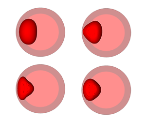
 The term in  ${f^{(2)}}$, which does not depend on time, describes the effect of average shape deformation. As one can see, independently of the density ratio, a compression of the inclusion in the direction of imposed vibrations takes place. The shape of the inclusion can be characterized by its smaller dimension ${b_x} = | {{x_C} - {x_A}} |$ and larger dimension ${b_y} = | {{y_B} - {y_D}} |$, where $A$ and $C$ denote the equatorial nodes, $B$ and $D$ the polar nodes (figure 1c). The ratio ${b_y}/{b_x}$ can thus be expressed as
 \begin{equation} \frac{b_y}{b_x} = \frac{{1 + {A^2}{{\tilde{\rho} }_l}{{\left( {{{\tilde{\rho} }_l} - {{\tilde{\rho} }_v}} \right)}^2}We/6}}{{1 - {A^2}{{\tilde{\rho} }_l}{{\left( {{{\tilde{\rho} }_l} - {{\tilde{\rho} }_v}} \right)}^2}We/6}}. \end{equation}
 The term in  ${f^{(2)}}$ depending on time is of resonance type: the oscillation amplitude unboundedly grows when the frequency approaches the resonance value. The eigen-frequencies of the inclusion oscillations are given by the formula (in our scaled units)
 \begin{equation} \varOmega_n^2 = \frac{1}{{We}}n({n^2} - 1),\quad n \geqslant 2, \end{equation}
a relation obtained by Lamb (Reference Lamb1881).
From similar but more cumbersome calculations for the cylindrical container of finite radius we obtain
 \begin{equation} \left.\begin{gathered} \varPhi_l^{(0)} = \frac{{\left( {{{\tilde{\rho} }_l} - {{\tilde{\rho} }_v}} \right)}}{{1 + {{(R/{R_c})}^2}\left( {{{\tilde{\rho} }_l} - {{\tilde{\rho} }_v}} \right)}}\left( {r + \frac{1}{r}} \right)\cos \theta \cos t,\quad\varPhi_v^{(0)} = 0,\quad {f^{(1)}} = 0, \\ F_s^{(2)} ={-} \frac{{{{\tilde{\rho} }_l}{{\left( {{{\tilde{\rho} }_l} - {{\tilde{\rho} }_v}} \right)}^2}}}{{6{{\left[ {1 + {{(R/{R_c})}^2}\left( {{{\tilde{\rho} }_l} - {{\tilde{\rho} }_v}} \right)} \right]}^2}}}We. \end{gathered}\right\}\end{equation}
It thus appears that, in the case of finite-size container, the dimensionless amplitude of the forced oscillations of the inclusion with respect to the laboratory reference frame is equal to
 \begin{equation} {A_{Lf}} = A\left( {1 + \frac{{\left( {{{\tilde{\rho} }_l} - {{\tilde{\rho} }_v}} \right)\left( {1 - {{(R/{R_c})}^2}} \right)}}{{1 + {{(R/{R_c})}^2}\left( {{{\tilde{\rho} }_l} - {{\tilde{\rho} }_v}} \right)}}} \right), \end{equation}
and with respect to the reference frame of the vibrating container it equals to
 \begin{equation} {A_{cf}} = A\frac{{\left( {{{\tilde{\rho} }_l} - {{\tilde{\rho} }_v}} \right)\left( {1 - {{(R/{R_c})}^2}} \right)}}{{1 + {{(R/{R_c})}^2}\left( {{{\tilde{\rho} }_l} - {{\tilde{\rho} }_v}} \right)}} = A\frac{{\left( {{{\tilde{\rho} }_l} - {{\tilde{\rho} }_v}} \right)}}{{{{\tilde{\rho} }_l}\dfrac{{1 + {{(R/{R_c})}^2}}}{{1 - {{(R/{R_c})}^2}}} + {{\tilde{\rho} }_v}}}. \end{equation}
The average shape deformation of the inclusion is written as
 \begin{equation} \frac{{{b_y}}}{{{b_x}}} = \frac{{1 + \delta }}{{1 - \delta }},\quad \delta = {A^2}\frac{{{{\tilde{\rho} }_l}{{\left( {{{\tilde{\rho} }_l} - {{\tilde{\rho} }_v}} \right)}^2}}}{{6{{\left[ {1 + {{(R/{R_c})}^2}\left( {{{\tilde{\rho} }_l} - {{\tilde{\rho} }_v}} \right)} \right]}^2}}}We. \end{equation}
 Thus, the average bubble shape deformation is determined by the dimensionless parameter  ${A^2}We$. Note that it can be also related to the Weber number as usually defined in the context of bubble dynamics if we choose $a = AR$ as the length scale in order to define the actual kinetic energy causing the bubble deformation.
The frequencies of eigen-oscillations of a cylindrical inclusion suspended in an inviscid liquid confined in a vibrating cylinder of finite radius are defined (in our scaled units) by the formula (Myshkis et al. Reference Myshkis, Babskii, Kopachevskii, Slobozhanin and Tyoptsov1987)
 \begin{equation} {\left( {\varOmega_n^ \pm } \right)^2} = \frac{1}{{We}}\frac{{n({n^2} - 1)}}{{\left( {{{\tilde{\rho} }_l}\kappa_n^2 + {{\tilde{\rho} }_v}} \right)}}, \end{equation}
where  $\kappa _n^2 = \coth ( {n\ln (q)} )$, $q = {R_c}/R$.
In Myshkis et al. (Reference Myshkis, Babskii, Kopachevskii, Slobozhanin and Tyoptsov1987) the damping rate of eigen-oscillations of a cylindrical inclusion suspended in a low-viscosity fluid of different density in a rotating cylindrical container of finite radius was calculated taking into account the effect of the viscous boundary layer. Based on the formulas obtained in Myshkis et al. (Reference Myshkis, Babskii, Kopachevskii, Slobozhanin and Tyoptsov1987), the following expression can be obtained for the damping rate of eigen-oscillations in the limit case of zero angular velocity of rotation:
 \begin{equation} {{\rm Re}} (\lambda_n^ \pm ) = n{\left( {1 - {q^{ - 2n}}} \right)^{ - 1}}\frac{{{{\tilde{\rho} }_l}\sqrt {{{\tilde{\nu} }_l}} }}{{\left( {{{\tilde{\rho} }_l}\kappa_n^2 + {{\tilde{\rho} }_v}} \right)}}\sqrt {\left| {\varOmega_n^ \pm } \right|} \left( {\frac{{{{\tilde{\rho} }_v}\sqrt {{{\tilde{\nu} }_v}} }}{{\left( {{{\tilde{\rho} }_v}\sqrt {{{\tilde{\nu} }_v}} + {{\tilde{\rho} }_l}\sqrt {{{\tilde{\nu} }_l}} }\, \right)}} + {q^{ - 2n - 1}}} \right)\delta_v^*, \end{equation}
where  $\delta _v^* = \sqrt {2({\nu _l} + {\nu _v})/\omega } /R$.
The formulas for infinitely large container are obtained from (2.31), (2.32) at  $q \to \infty$, ${\kappa _n} \to 1$
 \begin{align} {\left( {\varOmega_n^ \pm } \right)^2} = \frac{1}{{We}}n({n^2} - 1),\quad {{\rm Re}} (\lambda_n^ \pm ) = n\frac{{{{\tilde{\rho} }_l}\sqrt {{{\tilde{\nu} }_l}} }}{{\left( {{{\tilde{\rho} }_l} + {{\tilde{\rho} }_v}} \right)}}\sqrt {\left| {\varOmega_n^ \pm } \right|} \frac{{{{\tilde{\rho} }_v}\sqrt {{{\tilde{\nu} }_v}} }}{{\left( {{{\tilde{\rho} }_v}\sqrt {{{\tilde{\nu} }_v}} + {{\tilde{\rho} }_l}\sqrt {{{\tilde{\nu} }_l}} } \right)}}\delta_v^*. \end{align}
 Note that these formulas are valid for the parameter range satisfying the conditions  ${\delta _v} \ll 1$, $A \ll 1$, $R \ll c/\omega$. In the present work we study the behaviour of two different two-phase systems of liquid and its saturated vapour under isothermal conditions (SF $_6$ and parahydrogen p-H $_2$). The phase changes are not considered. The temperature for each of the systems is close to the critical point, such that the difference in the kinematic viscosities of phases can be neglected. At the same time, the distance from the critical point is not too small, such that both phases can be considered as incompressible. For both systems, experiments were carried out in microgravity conditions, for SF $_6$ in the Mir space station and for p-H $_2$ on Earth under gravity compensation by an inhomogeneous magnetic field.
3. Modelling and numerical approach
3.1. General
We consider a cylindrical cell filled with an isothermal two-phase system, liquid–vapour, without phase change, under the weightlessness condition  $g = 0$. The cell is submitted to a sinusoidal acceleration $\boldsymbol {\gamma }(t)$ of linear polarization in the plane perpendicular to the cylinder axis (figure 1)
 \begin{equation} {\boldsymbol{\gamma}} (t) = a{\omega ^2} {\boldsymbol{k}} \sin (\omega t + \varphi ). \end{equation}
The bubble motion and the deformation of its liquid–vapour interface is studied. In the numerical simulation it is assumed that the bubble is initially at the centre of symmetry of the container. Situations of high confinement are considered, i.e. the inclusion size is comparable to the container size. In the zero-gravity condition, without vibrational excitation, the vapour phase is a bubble of spherical shape. The temperature of the system is taken not too close to the critical temperature, such that both phases can be considered as incompressible; in addition, the densities of the phases are assumed to be comparable.
The case of an inclusion near a planar vibrating wall without the confinement effect has been previously investigated neglecting the viscosity by Lyubimov et al. (Reference Lyubimov, Lyubimova and Cherepanov1987), Lugovtsov & Sennitskiy (Reference Lugovtsov and Sennitskiy1987) and Lyubimov et al. (Reference Lyubimov, Cherepanov, Lyubimova and Avduevsky1992). It was shown that the wall attracts the inclusion, with a force that increases when the distance between the wall and inclusion decreases. For the two-phase configuration assumed in the present study (figure 1), one thus could expect that the bubble, initially located at the symmetry centre of the system, would be attracted preferably by the closest wall when vibration starts. For the vibrational velocity amplitudes exceeding some threshold, one can also expect parametric resonance oscillations of the L-V interface (Lyubimov et al. Reference Lyubimov, Lyubimova and Cherepanov2021).
3.2. Basic equations
One considers the isothermal flow of two immiscible fluids assumed to be viscous and Newtonian. The fluids are also assumed to be incompressible and homogeneous. Densities and viscosities are then constant within each fluid. A numerical investigation of the problem is carried out in the framework of a single fluid continuum model (Lyubimov & Lyubimova Reference Lyubimov and Lyubimova1990). In this case the governing equations of mass and momentum conservation of the fluid system written in the reference frame of the oscillating container can be written in dimensionless form as
 $$\begin{gather} \rho \left( {\frac{{\partial \boldsymbol{u}}}{{\partial t}} + \boldsymbol{u} \boldsymbol{\cdot} \boldsymbol{\nabla} \boldsymbol{u}} \right) ={-} \boldsymbol{\nabla} p + \boldsymbol{\nabla} \boldsymbol{\cdot} \left[ {\mu \left( {\boldsymbol{\nabla}\boldsymbol{u} + {\boldsymbol{\nabla}^T} \boldsymbol{u}} \right)} \right] + \rho {A_c}{\varOmega ^2} \boldsymbol{k} \sin (\varOmega t + \phi ) + La\,{\boldsymbol{F}_{\boldsymbol{\sigma}}}, \end{gather}$$
 $$\begin{gather}\boldsymbol{\nabla}\boldsymbol{\cdot}\boldsymbol{u} = 0 . \end{gather}$$
Here,  ${\boldsymbol {u}}$ denotes the velocity vector, $p$ is pressure, $\rho$ is the variable density, $\mu$ is the variable dynamic viscosity and $\boldsymbol {F_\sigma }$ is the surface tension force. The container radius, ${R_c}$, is chosen as the length scale, the viscous time, ${\tau _v} \approx R_c^2/\nu$ as the time scale, $\nu /{R_c}$ as the velocity scale and the quantities $({\rho _v} + {\rho _l})$ and $({\mu _v} + {\mu _l})$ respectively as the scales for the density and the dynamic viscosity of each fluid phase.
The equations contain the following dimensionless parameters: dimensionless vibration amplitude  ${A_c} = a/{R_c}$, dimensionless vibration frequency $\varOmega = 2{\rm \pi} fR_c^2/\nu$, the Laplace number $La = {\sigma {R_c}}/[{({\rho _v} + {\rho _l}){}{\nu ^2}}]$ representing the ratio of surface tension to the momentum transport and the dimensionless densities and viscosities. The ranges of these parameters for the problem under consideration are indicated in table 2 (SF $_6$ case) and table 5 (p-H $_2$ case).
Assuming that the surface tension is constant along the interface and adopting the continuum surface force (CSF) model (Brackbill, Koth & Zemach Reference Brackbill, Koth and Zemach1992), the interface is represented through the volume fraction field  $C$. In our discrete numerical implementation, $C$ is approximated by $\tilde {C}$, which represents a smooth transition across three to four grid elements (Popinet Reference Popinet2018). The surface tension force ${{\boldsymbol F}_\sigma }$ in the dimensionless form can then be written as follows:
 \begin{equation} {{\boldsymbol{F}}_\sigma } = K {\delta_S}\boldsymbol n\quad \text{with} \ K ={-} \boldsymbol{\nabla} \boldsymbol{\cdot} \boldsymbol n\quad \text{and} \quad \boldsymbol n = \frac{\boldsymbol{\nabla}\tilde{C}}{\left| {\boldsymbol{\nabla} \tilde{C}} \right|} . \end{equation}
Here,  $K$ is the local interface curvature, $\delta _S$ is the Dirac delta function localized on the interface and $\boldsymbol {n}$ is the unit vector normal to the interface. As in Kothe & Mjolsness (Reference Kothe and Mjolsness1992) and Popinet (Reference Popinet2018), we reformulate the CSF model by simply replacing the product of the delta function and the unit normal with the gradient of the smoothed volume fraction, ${\delta _S}{\boldsymbol {n}} \approx \boldsymbol {\nabla }\tilde {C}$. Steep gradients in the marker concentration $C$ represent the interface location. In a way equivalent to solving the advection of the phase-dependent density, one considers the advection of the $C$ function by the fluid velocity ${\boldsymbol {u}}$, governed by the relation
 \begin{equation} \frac{{\partial C}}{{\partial t}} + \boldsymbol{u} \boldsymbol{\cdot} \boldsymbol{\nabla} C = 0. \end{equation}
Here,  $0 \leqslant C \leqslant 1$, $C$ = 1 corresponds to the vapour phase, $C = 0$ is the liquid phase and $C = 0.5$ is the interface.
In the reference frame of the container, a no-slip boundary condition is imposed for the velocity field at the container walls. Along the symmetry axis  $(\kern0.7pt y = 0)$, classical symmetry boundary conditions are applied. A homogeneous Dirichlet boundary condition, $C = 0$, is applied along the container walls for the $C$ function. At initial time $(t = 0)$, the fluid is at rest and the vapour bubble is placed at the centre of the cylinder. The liquid–vapour interface is a coaxial cylinder.
In a single fluid continuum model context, the variable physical properties ( $\rho$ and $\mu$) are expressed by the following linear combinations (where subscript $v$ stands for vapour and $l$ for liquid):
 \begin{equation} \rho = C\frac{{{\rho_v}}}{{{\rho_v} + {\rho_l}}} + \left( {1 - C} \right)\frac{{{\rho_l}}}{{{\rho_v} + {\rho_l}}},\quad\mu = C\frac{{{\mu_v}}}{{{\mu_v} + {\mu_l}}} + \left( {1 - C} \right)\frac{{{\mu_l}}}{{{\mu_v} + {\mu_l}}} . \end{equation}
 The direct numerical simulation of our problem is restricted to a two-dimensional approach where the inclusion is assimilated to a vapour cylindrical column (figure 1a). In addition, one assumes that the fluid motion remains symmetrical with respect to the plane  $(\boldsymbol {z},\boldsymbol {k})$. The computational domain is thus restricted to the half-plane of the container section (see figure 1b), where $\boldsymbol {k}$ is parallel to $\boldsymbol {x}$.
3.3. Numerical approach
The governing equations are solved using a Galerkin finite-element method based on iso-parametric elements of Lagrange type. Space discretization relies on two-dimensional quadrilateral elements satisfying the Brezzi–Babuska stability condition (4-node linear element using bilinear interpolation functions for velocity components and a piecewise constant discontinuous pressure approximation with the pressure degree of freedom located at the centroid element) (Datt & Touzot Reference Datt and Touzot1984; Zienkiewicz, Taylor & Zhu Reference Zienkiewicz, Taylor and Zhu2013). The Eulerian description of the fluid motion is used in this work: structured conformal fixed mesh and symmetry with respect to the Oy axis.
The L-V interface is characterized by a volume of fluid type representation on the mesh (Hirt & Nichols Reference Hirt and Nichols1981; Liang Reference Liang1991). Advection and reconstruction of the fluid volume is performed by a volume tracking method (Rider & Kothe Reference Rider and Kothe1998; François et al. Reference François, Cummins, Dendy, Kothe, Sicilian and Williams2006). Starting from a given velocity field, the volume tracking method determines a new fluid interface (fluid volume advection and reconstruction steps). From the new fluid volume, the decoupled finite-element equations are then resolved sequentially in terms of primary variables to predict the kinematics. The reconstruction of the fluid volume within an element depends only upon its fill state and the fill of its neighbours (real and imaginary elements sharing a common side). During the advection step, a method referred to as advection adjustment (an alternative to flux limiting) is used in this work. The idea behind this method is to iteratively adjust the  $C$ marker to maintain it between 0 and 1 (with a cutoff value equal to $10^{-8}$, thus addressing a very small error to the overall mass balance. For the purpose of determining the behaviour of fluid at the mesh boundaries, imaginary neighbours are created along the exterior of the computational mesh and their influence is important. When they are full, a tracked fluid is reconstructed so that it contacts the mesh boundary. When they are empty, the corresponding construction leaves a small gap between the fluid and the boundary. Since it is assumed in the numerical model that the liquid completely wets the wall, there is no triple line.
Equations (3.3), (3.4) and (3.5) are solved using a temporal integration based on the first-order accurate implicit backward Euler scheme. A variable time increment is determined by the control of the local time truncation error  $\Delta t_u^{n + 1} / \Delta t_u^n = \sqrt { \varepsilon / {\| d^{n + 1} \|} }$ where the superscripts $n$ and $(n + 1)$ denote values from two consecutive time steps, $\Delta t_{u}$ is the hydrodynamic time step, $\varepsilon$ is a tolerance ( $\varepsilon = 10^{-3}$) and ${\| d ^{n + 1} \|}$ is the local time truncation error based on the predictor (forward Euler)/corrector (backward Euler) step (Gresho, Lee & Sani Reference Gresho, Lee, Sani, Taylor and Morgan1980). In (3.2), the surface tension in La is explicitly discretized in time, which introduces a capillary time step restriction (Galusinski & Vigneaux Reference Galusinski and Vigneaux2008; Popinet Reference Popinet2018; Ebo-Adou et al. Reference Ebo-Adou, Tuckerman, Shin, Chergui and Juric2019). In our relatively small-scale flow situation, this numerical stability condition can be slightly relaxed by the viscosity (Galusinski & Vigneaux Reference Galusinski and Vigneaux2008). Equation (33) is solved using an explicit first-order accurate forward Euler scheme.
A standard Courant–Friedrichs–Lewy condition is then used to limit the interface advection  $\Delta t_f= \textrm {CFL}\, h/|u|$, where CFL denotes the Courant number, $\Delta t_{f}$ stands for the kinematic equation time step and $h$ is an element size. A CFL value of the order of ${10^{-1}}$ or less is then chosen to satisfy the most restrictive capillary time step value. Our choice is motivated by the fact that the magnitude of the velocities generated by the capillarity is of the same order of magnitude as the magnitude of the induced translational vibrations velocities. They even remain somewhat lower throughout the study.
The time step taken for the full set of governing equations is simply chosen equal to the smallest time scales  $\Delta t = \min (\Delta {t_u},\Delta {t_f})$ satisfying thus the aforementioned numerical stability requirements. A sub-cycling strategy can also be used in the overall time stepping scheme, where multiple fluid advection steps are taken for a single velocity time step (Gresho et al. Reference Gresho, Lee, Sani, Taylor and Morgan1980).
Each conservation equation is solved separately in a sequential manner (segregated approach) (Haroutunian, Engelman & Hasbani Reference Haroutunian, Engelman and Hasbani1993). Each nonlinear flow equation is linearized using the fixed-point Picard method (also known as the successive substitution method) and a hybrid relaxation scheme (implicit and explicit factors) is employed to increase its asymptotically linear convergence rate. Combining the two components of the momentum equation with the continuity equation leads to an explicit equation for the pressure. The velocity–pressure coupling is then performed at discrete level using a simplified form for the pressure equation (less expensive in terms of computer memory). The efficient pressure projection (PP) algorithm (a finite-element counterpart of the SIMPLER algorithm) is used (Haroutunian et al. Reference Haroutunian, Engelman and Hasbani1993).
Linear iterative solvers are employed for solving each linearized sub-system (Saad Reference Saad2000). In addition to the conventional preconditioning, an implicit preconditioning is used to accelerate the convergence (Haroutunian et al. Reference Haroutunian, Engelman and Hasbani1993). The implicit preconditioning, performed before the conventional preconditioning, is achieved by using implicit relaxation of the non-symmetric advection-diffusion type linear equation systems and explicit relaxation of the pressure in the PP algorithm. A conjugate gradient (CG) solver with symmetric successive over-relaxation preconditioning is used for solving symmetric equation systems (pressure equation), and the conjugate gradient squared (CGS) solver with diagonal preconditioning is used for solving non-symmetric equation subsystems (advection-diffusion equations).
Since iterative solvers are used in the inner loop (instead of the direct Gaussian solver), the segregated approach requires an iterative process at two different levels and appropriate convergence criteria are required for each of these levels. For the outer loop, the convergence criterion used to stop the iterations is based on the relative variations of the primary variables  $\| \gamma _i - \gamma _{i-1} \| / \| \gamma _i \| \leqslant \varepsilon _u$ where the norm $\| \gamma \|$ is a root mean square norm summed over all the elements and computed separately for each degree of freedom $\gamma$, with i denoting the iteration index, and where $\varepsilon _u$ is a specified tolerance ${\varepsilon _u} = 10^{-4}$. The iterative solvers, CG and CGS, in the inner loop also require convergence criteria to terminate the iterative procedure before attempting convergence of the nonlinear iterations in the outer loop. Hence, a suitable convergence criterion, based on the normalized residual vector, is $\| \boldsymbol {R} ( u_i ) \|/ \| \boldsymbol {R} ( u_0 ) \| \leqslant \varepsilon _R$, where $\boldsymbol {R}(u_{0})$ is a reference vector and $\varepsilon _R = 10^{-4}$ is a specified tolerance.
An appropriate density and repartition of nodes is selected to deal with the presence of the vibrating wall and with the fact that the inclusion may exhibit relatively large displacements. A symmetrical structured conformal mesh with good orthogonality properties based on quadrilaterals is used. The maximal aspect ratio for a given cell is taken equal to  $2.5$ and the ratio between the smallest and the largest cell is taken equal to 5. For the entire set of simulations related to the SF $_6$ fluid, a mesh with 11 776 cells was employed and for the p-H $_2$ fluid, mesh sizes varying between 11 776 and 47 104 cells were used. Even less sensitivity of the results in the ortho-radial direction is observed (Lundgren & Mansour Reference Lundgren and Mansour1988; Basaran Reference Basaran1992), a maximal aspect ratio value equal to $5$ is maintained. The results were tested at different mesh sizes to verify mesh independency. An acceptable tolerance value representing $0.1\,\%$ relative variation of bubble deformation and length of periods of excited eigen-oscillations whenever possible was used (Basaran Reference Basaran1992; Meradji et al. Reference Meradji, Lyubimova, Lyubimov and Roux2001). In addition, according to the dimensionless Stokes boundary layers thicknesses mentioned in table 2 (for SF $_6$) and table 5 (for p-H $_2$), and to the grid cell sizes used in radial direction ( ${\sim }1\,\%$ of container radius for SF $_6$ and from ${\sim }0.05\,\%$ of container radius for higher vibration frequencies to $1\,\%$ for moderate ones in the case of p-H $_2$), 3–4 cells were used in the case of SF $_6$ (weak vibrations) and 4–6 cells in the case of p-H $_2$ (strong vibrations) to capture the viscous boundary layers. The simulation process requires between a few tens and a few hundred of time steps to describe every period of forcing oscillations. Several tens of forcing periods are necessary on average to reach a quasi-stationary position. In the context of a variable time stepping strategy, a maximal allowed value of the time step equal to 5 ms is imposed for a good compromise between accuracy requirement and computing cost. In practice, the time step can be lower than 1 ms, satisfying thus the numerical stability conditions. The usual CPU time using the sequential version of the implemented model is approximately 20 h for $5000$ time steps.
3.4. Parameters of the study
For a given vibrational excitation  $({A_c},\varOmega )$, the dimensionless inclusion radius $R/{R_c}$ is varied in the range 0.33–0.9. In the present two-dimensional (2-D) approach, the rate of volumic occupation of the vapour phase $\varphi = {\varphi _{V,3D}}$ is replaced by the rate of surfacic occupation ${\varphi _{S,2D}}$ in the median plane $(x,y)$. Let us compare this configuration with the experimental conditions where the bubble is a 3-D spherical bubble. According to the following (3.7a,b), with the same bubble radius $R/{R_c}$ the value ${\varphi _{V,3D}}$ would be smaller by the factor $(2/3)( {{R_c}/H} )( {R/{R_c}} )$, where $H$ represents the half-height of the cylindrical container
 \begin{equation} {\varphi_{S,2D}} = \frac{{{S_v}}}{{{S_v} + {S_l}}} = {\left( {\frac{R}{{{R_c}}}} \right)^2},\quad {\varphi_{V,3D}} = \frac{{{V_v}}}{{{V_v} + {V_l}}} = \frac{2}{3}\left( {\frac{{{R_c}}}{H}} \right){\left( {\frac{R}{{{R_c}}}} \right)^3} . \end{equation}
Here,  $S$ and $V$ denote the surface area in the median plane and the volume of the bubble, respectively. The 2-D inclusion, initially circular at the centre of the container, is subjected to a flattening in the vibration direction and becomes anisotropic. The shape of the vapour inclusion is characterized by its smaller dimension $b_{x}$ and larger dimension $b_{y}$ $(b_{x}=|x_{C}-x_{A}|, b_{y}=|y_{B}-y_{D}|$ in figure 1c). We will thus consider in the following the evolution of the ratio:
 \begin{equation} \frac{{{b_y}}}{{{b_x}}} = \frac{{\left| {{y_B} - {y_D}} \right|}}{{\left| {{x_C} - {x_A}} \right|}} . \end{equation}
 Two kinds of experimental conditions are considered, corresponding to fluids SF $_6$ and p-H $_2$, in different set-ups with different container sizes and for different vibrational conditions. The different bubble sizes investigated, corresponding to various surfacic fraction ${\varphi _{S,2D}}$ and volumic fraction $\varphi _{V,3D}$, are reported in tables 2 and 5.
4. Weak vibrations (SF $_6$)
$_6$)

The data on the physical properties of SF $_6$ used in the simulation are given in table 1. Temperature is assumed uniform at $T = T_{c} -100$ mK with $T_{c} = 318.69$ K. The experimental set-up (ALICE-2) is described in detail in Marcout et al. (Reference Marcout, Zwilling, Laherrere, Garrabos and Beysesn1995), Polezhaev et al. (Reference Polezhaev, Emelianov, Ivanov, Kalmykov, Beysesn and Garrabos2001) and Garrabos et al. (Reference Garrabos, Beysens, Lecoutre, Dejoan, Polezhaev and Emelianov2007).
Table 1. Physical properties of SF $_6$ (Zappoli, Beysens & Garrabos Reference Zappoli, Beysens and Garrabos2015).

In table 2 the geometrical and vibrational parameters of the experiments with SF $_6$ are presented in dimensional and non-dimensional forms. The values of non-dimensional parameters are calculated taking the scales as the ones used in the direct numerical simulations (DNS); such scales are chosen in the numerical modelling since ${R_c}$ and $\nu$ remain constant for each system (SF $_6$ and p-H $_2$), whereas the inclusion radius and the vibration frequency are varied.
Table 2. Geometrical and vibrational conditions for the simulation of SF $_6$ experiment. N.D. stands for non-dimensional (see text).

For comparison with the analytical formulas obtained under the assumptions of small-amplitude high-frequency vibrations one needs to have  ${A_c} \ll 1$, $\varOmega \gg 1\ ({\delta _v} \ll 1)$. As we will see, these restrictions are satisfied in these experiments. Thus, their results can be successfully described by the theory developed in the small-amplitude and high-frequency (low-viscosity) approach.
The dimensionless average vibrational force (per unit of cylinder length), which is responsible for the average displacement of the bubble to the nearest wall, is small enough for SF $_6$ experiment. One thus could expect small average bubble displacement due to this force. Because of that we call the vibrational conditions in the SF $_6$ experiment weak vibrations.
4.1. Bubble displacement
The displacement of the bubble is characterized by the evolution of the position of its centre of mass (centroid),  $x_g$. The numerical results on the temporal evolution of the bubble centroid position for two different initial phases $\phi = 0$, $\phi = {\rm \pi}/2$ are shown in figures 2(a) and 2(b), respectively. As one can see, in both cases the bubble undergoes forced translational oscillations with the frequency equal to the frequency of the imposed vibrations.

Figure 2. Evolution of the bubble centre of mass  $(x_g)$ for different dimensionless bubble radii $R/{R_c}$ in SF $_6$ at ${A_c} = 0.0667$, $\varOmega = 3.6 \times {10^3}$: (a) $\phi = 0$, (b) $\phi = {\rm \pi}/2$.
Numerical data on the amplitude of these oscillations are well described by (2.29) obtained for the dimensionless amplitude of bubble oscillations in the reference frame of an oscillating container. Indeed, substituting the values of the dimensionless amplitude of the imposed vibrations and the dimensionless densities of the two-phase system under consideration, one obtains for the case  $R/{R_c} = 1/2$ the value ${A_{cf}} \approx 0.0057$ (in the container radius units). Analysis of the results of direct numerical simulation gives ${A_{cf}} \approx 0.0062$.
Additionally to the translational forced oscillations, the bubble is subjected to an average displacement. In the case  $\phi = 0$, a considerable average displacement of the bubble centroid from the container centre is observed. This displacement continues until the bubble reaches the vicinity of a wall. In the case $\phi = {\rm \pi}/2$, the initial impulse leads to some average displacement of the bubble centroid from the container centre. However, in the course of further oscillations, a gradual return to the container centre is observed. At large time scales, stationary oscillations occur around the average position at the symmetry centre.
The system therefore demonstrates quite different behaviours in the cases  $\phi = {\rm \pi}/2$ and $\phi = 0$. This difference concerns not only the behaviour at small time scales but also the asymptotic limit behaviour at large time scales.
4.2. Discussion and explanation by a simple mechanical model
Some features of the bubble behaviour observed in the DNS can be understood by using a simple mechanical model. If one neglects the bubble deformation and the wall influence, one can write an equation for motion in the following form:
 \begin{equation} m\ddot{x} + \alpha \dot{x} ={-} \chi ma{\omega ^2}\sin (\omega t + \phi ) . \end{equation}
Here,  $m$ is the sum of the inclusion mass and added mass, $\alpha$ is an effective friction coefficient, $V$ is the volume of inclusion and $\chi = ( {{\rho _l} - {\rho _v}} )V/m$. The phase $\phi$ has the same meaning as in the DNS case.
By choosing  ${\omega ^{ - 1}}$ as the time scale and the product $(a \chi )$ as the length scale, the equation of the inclusion motion can be written in the dimensionless form as
 \begin{equation} \ddot{x} + \bar{\alpha}\dot{x} ={-} \sin \left( {t + \phi } \right). \end{equation}
Here, the same notations are kept for the dimensionless time and coordinate and  $\bar {\alpha } = \alpha /(m\omega )$ is the dimensionless friction coefficient. Equation (4.2) is written in the reference frame of the container such that $x$ represents the bubble displacement from the container centre.
The initial conditions at  $t = 0:\,x = 0$, $\dot {x} = 0$.
The solution to the problem is
 \begin{equation} x = \frac{{{{\bar{\alpha} }^2}\cos \left( {t + \phi } \right) - {{\bar{\alpha} }^2}\cos \left( \phi \right) - {{\rm e}^{ - \bar{\alpha} t}}\sin \left( \phi \right)\bar{\alpha} + \bar{\alpha} \sin \left( {t + \phi } \right) - \cos \left( \phi \right) + {{\rm e}^{ - \bar{\alpha} t}}\cos \left( \phi \right)}}{{\left( {{{\bar{\alpha} }^2} + 1} \right)\bar{\alpha} }} . \end{equation}
4.2.1. Inviscid regime
In the limit case  $\bar {\alpha } \to 0$ (4.3) gives
 \begin{equation} x = \sin \left( {t + \phi } \right) - t\cos \left( \phi \right) - \sin \left( \phi \right) . \end{equation}
 According to (4.4), a continuous motion of the bubble from the container centre is thus observed for  $\phi = 0$ (figure 3a) while, for $\phi = {\rm \pi}/2$ the bubble oscillates around a non-zero value (figure 3b).

Figure 3. Evolution of the bubble position in the absence of friction (4.4). Panels show (a)  $\phi = 0$, (b) $\phi = {\rm \pi}/2$. Here, $x$ and $t$ are dimensionless (see text).
4.2.2. Influence of friction
The presence of friction substantially modifies the behaviour. For  $\bar {\alpha } \to \infty$ the bubble does not move. This is due to the fact that, when the viscosity tends to infinity, the properties of the fluid tend to the properties of an absolutely solid body. If the initial bubble velocity were non-zero, the bubble velocity would decrease instantaneously to zero, due to an infinite friction force. For very large but finite viscosity one obtains an asymptotic behaviour in the form of damped exponential without oscillations. Indeed, when the viscosity is very high, the inclusion does not have enough time to make even one oscillation, the time decay being very fast. The evolution of the bubble position described by (4.3) was directly compared with the results of DNS. Figure 4 shows the superposed graphs obtained from (4.3) with $\bar {\alpha } = 0.125$ and by DNS at $R/{R_c} = 1/2$ for $\phi = 0$ and $\phi = {\rm \pi}/2$. Both graphs are presented in the dimensionless form using the scales introduced in the § 4.2. As one can see, the results are in a quite good agreement. For $\phi = 0$, the bubble quickly moves away from the centre of the container at the beginning of the process, as in the case without friction, but reaches a final equilibrium position around which oscillations can be seen. For $\phi = {\rm \pi}/2$, one observes the bubble moving back to the centre, its position at late times being ${x_g} = 0$.

Figure 4. Evolution of the bubble centre of mass for (a)  $\phi = 0$ and (b) $\phi = {\rm \pi}/2$ in the presence of friction. The DNS results for SF $_6$ fluid at $(T-T_c)=-100$ mK, $R/{R_c} = 1/2$, ${A_c} = 0.0667$, $\varOmega = 3.6 \times {10^3}$ vs the mechanical model predictions (theory) for $\bar {\alpha } = 0.125$.
4.3. Evolution of the bubble shape
4.3.1. Case $\phi = 0$

The evolution of the bubble shape can be represented by the time dependence of the aspect ratio  ${b_y}/{b_x}$ of the ellipse that approximately describes the bubble shape (see figure 1c). For the case $\phi = 0$, the evolution of the aspect ratio is presented in figure 5. The ratio ${b_y}/{b_x}$ remains always larger than unity, indicating a flattening in the vibration direction $x$, as predicted in Lyubimov et al. (Reference Lyubimov, Cherepanov and Lyubimova1996, Reference Lyubimov, Cherepanov, Lyubimova and Roux1997). For bubbles of smaller size $R/{R_c} = 0.5$ and $0.7$, the flattening appears to be very important at the early times, where ${b_y}/{b_x}$ exhibits damped oscillations of large pseudo-period compared with the imposed vibration period. These oscillations apparently correspond to the eigen-oscillations of the bubble, which are damped with time. After this transitory oscillatory regime, ${b_y}/{b_x}$ reaches an asymptotic value, representing the permanent regime. This asymptotic value increases with the ratio $R/{R_c}$, in agreement with the theoretical predictions in Lyubimov et al. (Reference Lyubimov, Cherepanov and Lyubimova1996). All curves also present oscillations of small amplitudes and forcing frequency. These oscillations correspond to the quadrupole mode which is usually dominant in the shape deformation. The oscillations are attenuated for bubbles of large size, probably due to an effect of confinement. For the largest bubble ( $R/{R_c} = 0.9$), the asymptotic behaviour is not obtained after dimensionless time equal to $0.278$ (100 s). The reason can be found in the dependence of the period of eigen-oscillations on the bubble radius (see (2.31)).

Figure 5. Evolution of the aspect ratio  ${b_y}/{b_x}$ of the bubble (assimilated to an ellipse), for different $R/{R_c}$. Fluid SF $_6$,
$_6$,  $\phi = 0$, ${A_c} = 0.0667$, $\varOmega = 3.6 \times {10^3}$.
4.3.2. Case $\phi ={\rm \pi} /2$

Figure 6 shows the evolution of the ratio  ${b_y}/{b_x}$, $\phi = {\rm \pi}/2$. Similar to the case $\phi = 0$, at early times one observes a damped oscillatory behaviour for small size bubbles ( $R/{R_c}=0.5$ and $0.7$). The oscillations presumably correspond to the viscous damping of the eigen-oscillations of the bubble. One notes that the (quadrupole) oscillations at forcing frequency, clearly visible in the former case of § 4.3.1 where $\phi = 0$ (figure 5), become now hardly visible. This is related to the fact that, as seen from figures 2(a)–2(b), in the case $\phi = 0$, the bubble is subjected to a fast average displacement from the container centre whereas at $\phi = {\rm \pi}/2$, the average displacement of the bubble is very small.

Figure 6. Evolution of the aspect ratio,  ${b_y}/{b_x}$ of the bubble (assimilated to an ellipse), for different dimensionless bubble radii $R/{R_c}$; fluid SF $_6$;
$_6$;  $\phi = {\rm \pi}/2$, ${A_c} = 0.0667$, $\varOmega = 3.6 \times {10^3}$.
4.3.3. Aspect ratio estimation
As shown in § 2 (see also Lyubimov et al. Reference Lyubimov, Cherepanov and Lyubimova1996, Reference Lyubimov, Cherepanov, Lyubimova and Roux1997), and already discussed in §§ 2, 4.2.1 and 4.2.2, under the action of vibrations the inclusion is subjected to an average shape deformation – flattening in the direction of the vibration axis. The average shape deformation of a cylindrical bubble in a cylindrical container of finite size is defined by (2.30a,b). This expression is obtained from a perturbation theory and is valid within the assumptions of high frequency of vibrations (low viscosity)  $\varOmega \gg 1\ ({\delta _v} \ll 1)$, ${A_c} \ll 1$.
The above relationship does not depend on the initial phase  $\phi$. Comparisons of the ${b_y}/{b_x}$ values as calculated from (2.30a,b) and resulting from DNS are shown in table 3. As one can see, the agreement is within a few per cent.
Table 3. Ratio  ${b_y}/{b_x}$. Comparison between (2.30a,b) and numerical simulations.

4.3.4. Pseudo-periods
The pseudo-periods and damping rate obtained in the calculations can be compared with the characteristics of a free oscillating bubble. Let us consider the second mode  $n = 2$ (quadrupole deformation), which is usually dominant in the interface deformations. For this mode, with $R/{R_c} = 1/2$, (2.31) and (2.32) give a period of oscillations of $T = 0.034~(12.3$ s $)$ and damping time ${T_d} \approx 0.050\ (17.9\ \textrm {s})$. Processing the results of DNS presented in figure 6 we obtain $T = 0.034\ (12.3\ \textrm {s})$ for the period of oscillations and ${T_d} \approx 0.033\ (12.0\ \textrm {s})$ for the damping time. Note that, (2.31) and (2.32) give the frequency and damping time for free oscillations in the absence of forcing and figure 6 presents the results of DNS for temporal evolution of the bubble shape (in terms of aspect ratio) for oscillations of the bubble under the influence of forced vibrations, so we see superposition of the eigen and forced oscillations which finally (when eigen-oscillations are completely damped) results in the elliptical quasi-equilibrium average shape of the bubble (in our case, with the aspect ratio equal approximately to $1.1$). Thus, the agreement of analytical and DNS results could be considered as good enough.
Non-monotonic behaviour can be expected for all values of  $R/{R_c}$. However, the eigen-oscillation period increases with $R/{R_c}$, as shown by (2.31). The time needed to observe such oscillations becomes very large for the bubbles of the largest sizes ( $R/{R_c} = 0.8$ and $0.9$). This time becomes comparable to or larger than the damping time. Then the oscillatory regime is over-damped and is not observed, even after large simulation times (see figures 5 and 6).
4.3.5. Comparison with experiment
The results of calculations for SF $_6$ were compared with the experiments performed at the MIR station in parallel with the study of Garrabos et al. (Reference Garrabos, Beysens, Lecoutre, Dejoan, Polezhaev and Emelianov2007). In figure 7 experimental photos obtained in these experiments are presented (these photos were kindly presented to us by the PI of the experiment). The left picture shows the bubble in the absence of vibrations and the right picture shows the bubble under vibrations at frequency 1.6 Hz and amplitude 0.8 mm. As one can see, under the action of vibrations the bubble is elongated in the direction perpendicular to the vibrations. This is due to the orienting effect of vibrations formulated for the first time in Lyubimov et al. (Reference Lyubimov, Cherepanov, Lyubimova and Roux1997): under the influence of vibrations, the surfaces of constant density are oriented perpendicular to the direction of vibrations. From (2.30a,b) for the parameter values used in the experiment one obtains the mean aspect ratio of the bubble equal to 1.57. Note, however, that (2.30a,b) is valid for $A \ll 1$ (dimensional vibration amplitude is much smaller than the bubble radius) and in the experiment $A \approx 0.178$, which is beyond the applicability of (2.30a,b). That is why one should expect anoverestimated value of ${b_y}/{b_x}$ from (2.30a,b). From figure 5 one obtains ${b_y}/{b_x} = 1.35$, which allows us to conclude that there is good enough agreement.

Figure 7. An SF $_6$ bubble (underlined by interrupted circle or ellipse) for $(T-T_c)= -113$ mK and $R/R_c = 0.75$. (a) At equilibrium, (b) submitted to a harmonic vibration with frequency 1.6 Hz and amplitude 0.8 mm; double arrow indicates the vibration direction – experiment in MIR station carried out in parallel with the study by Garrabos et al. (Reference Garrabos, Beysens, Lecoutre, Dejoan, Polezhaev and Emelianov2007). With the courtesy and permission of D. Beysens.
4.4. Summary
The main difference between the results obtained for SF $_6$ in the cases $\phi =0$ and $\phi ={\rm \pi} /2$ appears in the average displacement of the bubble. The bubble centre of mass oscillates at the centre of the container for $\phi = {\rm \pi}/2$ and moves away from the centre for $\phi =0$. The reason for this difference can be explained using a simple mechanical model. There is no major difference between the cases $\phi = 0$ and $\phi = {\rm \pi}/2$ concerning the aspect ratio $b_y/b_x$ of the bubble. One observes in both cases a transitory regime of similar nature and period. One notes, however, a slight difference. In the case $\phi = 0$ small oscillations are superimposed onto the main evolution of the aspect ratio, in contrast to the case $\phi = {\rm \pi}/2$ where these oscillations are not visible. This could be related to the fact that, as is seen from figures 2(a) and 2(b), in the case $\phi = 0$ the bubble is subjected to a fast average displacement from the container centre whereas, at $\phi = {\rm \pi}/2$, this displacement remains very small.
5. Strong vibrations (p-H$_2$)

This section deals with a vapour bubble under vibrations as used in the experiments with parahydrogen. Typical values of the parameters are chosen to correspond at best to both the experimental data and the simulation constraints.
5.1. The physical properties of p-H$_2$

The experiments with hydrogen were performed at the typical cryogenic temperatures of 500 mK and 200 mK below the critical temperature  ${T_c} = 33.19$ K. When p-H $_2$ is cooled in the cell, the normal-H $_2$ (n-H $_2$)–para-H $_2$ (p-H $_2$) equilibrium is shifted and the percentage of p-H2 increases from $25\,\%$ at room temperature to $96\,\%$ at $30$ K, with a time constant of approximately 50 h (Wunenburger et al. Reference Wunenburger, Chatain, Garrabos and Beysens2000). In the conditions where the experiments were carried out, the H $_2$ was in its p-state. The useful data are summarized in table 4.
Table 4. Physical properties of p-H $_2$ (Jouers Reference Jouers1986; Zappoli et al. Reference Zappoli, Beysens and Garrabos2015). The subscript $l$ denotes liquid and $v$, vapour.

5.2. Numerical simulation scenarios
The conditions used to simulate the experiments with  ${A_c} = 0.0333\unicode{x2013} 0.267$ ( $a = 0.05\unicode{x2013} 0.4\ \textrm {mm}$) and $\varOmega = 2.64 \times {10^3}\unicode{x2013} 5.95 \times {10^3}~(f = 20\unicode{x2013} 45\ \textrm {Hz})$ are given in table 5.
Table 5. Geometrical and vibrational conditions for the simulation of the p-H $_2$ experiment. N.D. stands for non-dimensional (see text).

As one can see, the restrictions  ${A_c} \ll 1$, $\varOmega \gg 1\ ({\delta _v} \ll 1)$ are satisfied for this experiment too. Vibrations could be thus considered as being of (i) small amplitude and (ii) high frequency and the results can be successfully described by the theory developed in the small-amplitude and high-frequency (low-viscosity) approach.
The dimensionless average vibrational force (per unit of cylinder length), which is responsible for the average displacement of the bubble to the nearest wall, is much larger than for the SF $_6$ experiment. One thus could expect much larger average displacement of the bubble due to this force. Because of this we call the vibrational conditions in the p-H $_2$ experiment ‘strong vibrations’.
In Lyubimov et al. (Reference Lyubimov, Lyubimova and Cherepanov2021) it was shown that the forced oscillations of a spherical drop or bubble surrounded by a fluid of different density under vibrations of non-acoustic frequency with linear polarization can become unstable with respect to the parametrically excited oscillations, represented by the superposition of drop eigen-oscillations. In the absence of viscosity, the most easily excited oscillations are the oscillations which satisfy the synchronism condition
 \begin{equation} {\varOmega_r} = {\varOmega_n} + {\varOmega_{n + 1}} . \end{equation}
Here,  ${\varOmega _r}$ is the dimensionless resonance frequency and ${\varOmega _n}$ and ${\varOmega _{n + 1}}$ are the dimensionless frequencies of two neighbouring modes of eigen-oscillations.
In (5.1) two neighbouring modes are involved because their interaction is performed through a translational mode. In this sense, the condition for the excitation of the parametric resonance should be the same for spherical and cylindrical inclusions. Accordingly, in the case of the cylindrical bubble studied in the present paper by DNS, one should also expect the excitation of the parametric resonance when the synchronism condition equation (5.1) is satisfied.
Substituting the values of the eigen-frequencies calculated from (2.31) for the two-phase system p-H $_2$ at $(T-T_c)=-500$ mK in (5.1), one obtains for $R/{R_c} = 1/2$: ${\varOmega _2} = 1.63 \times {10^3}$, ${\varOmega _3} = 3.36 \times {10^3}$, ${\varOmega _{r2,3}} = 4.99 \times {10^3}$ $(\,{f_2} \approx 12.3\ \textrm {Hz}, {f_3} \approx 25.5 \ \textrm {Hz}, {f_{res,2\unicode{x2013} 3}} \approx 37.8\ \textrm {Hz})$. At $(T- {T_c})= -200$ mK, one obtains from (2.31) for $R/{R_c} = 1/2$: ${\varOmega _2} = 0.916 \times {10^3}$, ${\varOmega _3} = 1.89 \times {10^3}$, ${\varOmega _{r2,3}} = 2.81 \times {10^3}$ ( ${f_2} \approx 6.93\ \textrm {Hz}, {f_3} \approx 14.3\ \textrm {Hz}$, ${f_{res,2\unicode{x2013} 3}} \approx 21.2\ \textrm {Hz}$).
A few scenarios in terms of vibration frequency and amplitude have been chosen for two small size bubbles ( $R/{R_c} = 0.50\ \textrm {{and}}\ 0.33$) taking into account the conditions of the linear stability analysis in Lyubimov et al. (Reference Lyubimov, Lyubimova and Cherepanov2021) and the above frequency calculations. In the first scenario, the vibration frequencies were chosen with respect to the resonance condition for each bubble size $R/{R_c}$. Most of the scenarios therefore consist of varying the vibration amplitude around the threshold value beyond which parametric oscillations are expected. As already noted, for reasons of drop stability, the vibration amplitude had to be limited ${A_c} = [0.0333\unicode{x2013} 0.333]\ (a = [0.05\unicode{x2013} 0.50]\ \textrm {mm})$. The other scenario consists of varying the vibration frequency for a given value of the amplitude.
5.3. Discussion of the numerical results
The numerical simulations have been performed for the vibrational parameters (amplitude and frequency) and the physical properties and geometrical conditions given in tables 4 and 5. The comparison between the solutions corresponding to  $\phi = 0$ and $\phi = {\rm \pi}/2$ has been performed only for a few pairs of $({A_c},\varOmega )$ values.
Figures 8–10 illustrate the evolution of the bubble centroid position at different amplitudes and frequencies of the container vibrations, bubble sizes and initial phases. In figure 8 the evolution of the bubble centroid position is described for  $(T-{T_c}) = -500$ mK, $~\phi = {\rm \pi}/2$, $R/{R_c} = 1/2$, $\varOmega = 5.09 \times {10^3}\ (f = 38.5\ \textrm {Hz})$ and different values of the dimensionless vibration amplitude ${A_c}$.

Figure 8. Evolution of the bubble centre of mass,  ${x_g}$ for $\phi = 0$ and different values of the non-dimensional vibration amplitude ${A_c}$. Fluid p-H $_2$ at $(T-T_{c}) = -500$ mK. Here, $\varOmega = 5.09 \times {10^3}\ (f = 38.5\ \textrm {Hz})$, $R/{R_c} = 1/2$.

Figure 9. Evolution of the bubble centre of mass,  ${x_g}$, for different values of non-dimensional vibration amplitude ${A_c}$. Fluid p-H $_2$,
$_2$,  $R/{R_c} = 1/2$, case $\phi ={\rm \pi} /2$. Panels show (a) $(T-T_{c}) = -500$ mK, $\varOmega = 5.09 \times {10^3}\ (f = 38.5\ \textrm {Hz})$; (b) $(T-T_{c}) = -200$ mK, $\varOmega = 2.64 \times {10^3}\ (f = 20\ \textrm {Hz})$.

Figure 10. Evolution of the bubble centre of mass,  ${x_g}$, for different values of dimensionless frequency $\varOmega$. Fluid p-H $_2$ at $(T-T_{c}) = -500$ mK, $\phi = {\rm \pi}/2$, ${A_c} = 0.167\ (a = 0.25\ \textrm {mm})$ and $R/{R_c} = 1/2$.
The bubble moves on average from the container centre to one of the walls. This average displacement is due to appearance of an average vibrational force acting on the bubble from the oscillating liquid. As shown in Lyubimov et al. (Reference Lyubimov, Cherepanov, Lyubimova and Roux2001a) for the case of a flat wall, a cylindrical inclusion located at a distance  $d$ from the wall in an inviscid oscillating fluid is attracted to the wall by the following force:
 \begin{equation} F = \frac{{\rm \pi} }{2}\frac{{{a^2}{\omega ^2}R{\rho_l}{{({\rho_l} - {\rho_v})}^2}}}{{{{({\rho_l} + {\rho_v})}^2}}}{\left( {\frac{d}{{{R_c}}}} \right)^{ - 3}} . \end{equation}
Due to the symmetry of the system, the average vibrational force vanishes when the inclusion is located in the container centre. This state corresponds to an unstable equilibrium. When the inclusion is displaced from the centre, even slightly, a non-zero mean vibrational force appears and the inclusion starts to move (on average) to one of the walls (figures 8–10). Additional calculations with the initial position of the bubble slightly shifted from the centre were carried out. They show that, in such a case, the bubble is always subjected to an average displacement in the same direction.
As seen from tables 2 and 5, the dimensionless average vibrational attraction force for the p-H $_2$ experiment conditions is much larger than for SF $_6$. This explains why the average displacement, not pronounced in the case of weak vibrations for SF $_6$, turns out to be considerable in the case of strong vibrations for p-H $_2$.
$_2$.
Equation (5.2) for the average vibrational force has been obtained by neglecting the viscosity and is valid at a not too small inclusion–wall distance. In the vicinity of the wall, viscous effects become important. As shown in Klotsa et al. (Reference Klotsa, Swift, Bowley and King2007) and Lyubimova et al. (Reference Lyubimova, Lyubimov and Shardin2011), for the case of interaction of two inclusions in a viscous oscillating fluid (when the vibration axis is perpendicular to the line connecting the inclusions), the interaction force changes its sign with the decrease of distance between the inclusions. At small distances the inclusions therefore repulse each other. The ‘equilibrium’ distance where the interaction force changes its sign is proportional to the viscous Stokes layer thickness.
A similar behaviour should be also observed in the case of a wall–inclusion interaction. The average displacement of an inclusion to the nearest wall in a viscous fluid subjected to vibrations should therefore stop at an ‘equilibrium’ distance from the wall, a distance which decreases with increasing frequency. Before stopping (on average) at this quasi-equilibrium position, the bubble performs around this site damped oscillations with large amplitude and large period due to the elastic properties of the bubble surface. At high frequencies of vibrations, the viscous Stokes layer is very thin. In this case, the bubble eventually locates just at the wall and its surface performs small-amplitude forced oscillations with vibration frequency. These phenomena are observed in figures 8–10.
5.3.1. Bubble displacement for $\phi = 0$

The evolution of  ${x_g}$ in the case $R/{R_c} = 1/2$ is shown in figure 8. As one can see, all the curves exhibit oscillations of small amplitude with frequency equal to the forcing frequency. In addition to these forced oscillations, the inclusion shows a well-defined behaviour at larger time scale. Similar to the case of weak vibrations, the inclusion, initially placed at the centre, is immediately propelled in the direction of initial impulse $x<0$. Then, it exhibits different behaviour: (i) for larger values of the dimensionless vibration amplitude, the inclusion moves (on average) towards the wall and stabilizes there in quasi-contact with the vibrating wall $(| {{x_g}} | \approx 0.533)\ (0.8\ \textrm {mm})$ to be compared with $({R_c} - R)/{R_c} = 0.5\ (0.75\ \textrm {mm})$; (ii) for lower values of ${A_c}$, large-scale oscillations around some quasi-equilibrium position at finite distance from the wall occur and are progressively damped, with some tendency for the bubble to stabilize at this position.
5.3.2. Bubble displacement in the case $\phi = {\rm \pi}/2$

In this case, both amplitude and frequency are varied at a constant bubble volume fraction ( $R/{R_c} = 1/2$).
Variable amplitude
Figure 9 shows the evolution of the centre of mass for various values of  ${A_c}$ and temperatures $(T-T_{c})$ and two frequencies. For $\varOmega = 5.09 \times {10^3}\ (f = 38.5\ \textrm {Hz})$ (figure 8a) and $(T-T_{c}) = -500$ mK, the corresponding velocities are in the range ${A_c}\varOmega = [1.68 \times {10^2}\unicode{x2013} 8.40 \times {10^2}]$ $(1.2\ \textrm {cm}\ \textrm {s}^{-1} \leqslant a\omega \leqslant 6.0\ \textrm {cm}\ \textrm {s}^{-1})$. In contrast to the $\phi = 0$ case, and similar to the case of weak vibrations at $\phi = {\rm \pi}/2$, the bubble is not immediately propelled in the $x<0$ direction. The centre of mass oscillates in the vicinity of the centre during a time equal to 5–6 forcing periods (i.e. approximately $0.0076$ or $0.16$ s). Then, the $x{}_g$ evolution exhibits the following behaviour, depending on ${A_c}$:
(i) For larger values of the dimensionless vibration velocity amplitude
$0.117 < {A_c} < 0.167$ $(0.175\ \textrm {mm} < a < 0.25\ \textrm {mm})$, i.e. $5.89 \times {10^2} \leqslant {A_c}\varOmega \leqslant 8.41 \times {10^2}$ $(4.2\ \textrm {cm}\ \textrm {s}^{-1} < a\omega < 6.0\ \textrm {cm}\ \textrm {s}^{-1})$ the initial position being unstable, the inclusion is attracted by the closest vibrating wall. This result is in agreement with the theoretical prediction in Lyubimov et al. (Reference Lyubimov, Lyubimova and Cherepanov1987), where an inclusion should move in the direction of the initial acceleration. When ${A_c}$ increases, one observes a progressive lowering of the damping time, the inclusion coming into quasi-contact with the wall. This is especially true for the largest vibration amplitude ($| {{x_g}} | \approx 0.5\unicode{x2013} 0.57$) to be compared with $({R_c} - R)/{R_c} = 0.5\ (0.75\ \textrm {mm})$. Figure 8(a) also shows that the forced oscillation amplitude increases with ${A_c}$ for a given value of $\varOmega$, a behaviour expected from (2.29).(ii) For smaller values of the dimensionless vibration amplitude
$0.0333 \leqslant {A_c} \leqslant 0.1$ $(0.05 \textrm {mm} \leqslant a \leqslant 0.15\ \textrm {mm})$, i.e. ${A_c}\varOmega = [1.68 \times {10^2}\unicode{x2013} 5.09 \times {10^2}]$ $(1.2\ \textrm {cm}\ \textrm {s}^{-1} \leqslant$ $a\omega \leqslant 3.6\ \textrm {cm}\ \textrm {s}^{-1})$ the inclusion moves on average towards the $x>0$ side (opposite to the initial acceleration). This displacement is accompanied by the forced oscillations. At a later stage, one sees a tendency of stabilization of the inclusion position at some distance from the centre which becomes closer and closer to the centre with the decrease of the vibration amplitude $| {{x_g}} | = [0.5\unicode{x2013} 0.567]\ (0.75\unicode{x2013} 0.85\ \textrm {mm})$, to be compared with $({R_c} - R)/{R_c} = 0.5\ (0.75\ \textrm {mm})$.


Figure 9(b) corresponds to a situation closer to the experimental configuration, with  $(T-T_{c}) = -200$ mK and $\varOmega = 2.64 \times {10^3}\ (f = 20\ \textrm {Hz})$. The corresponding vibration velocity amplitudes are in the range $4.41 \times {10^2} \leqslant {A_c}\varOmega \leqslant 7.05 \times {10^2}$ $(3.1\ \textrm {cm}\ \textrm {s}^{-1} < a\omega < 5.0\ \textrm {cm} \textrm {s}^{-1})$. The same behaviour as above is found. In particular, the range of amplitudes where large-amplitude damped oscillations with large period are observed is the same; they are observed for the lowest vibration amplitudes. For ${A_c} = 0.267$, i.e. ${A_c}\varOmega = 7.05 \times {10^2} \ (a = 0.40\ \textrm {mm}$, i.e. $a\omega = 5.0\ \textrm {cm}\ \textrm {s}^{-1}$) the bubble moves in the $x < 0$ direction up to $t \approx 0.047\ (1\ \textrm {s})$; then, it stabilizes at $x_g \approx 0.547\ (0.82 \ \textrm {mm})$. For ${A_c}=0.2$ ${A_c}\varOmega = 5.28 \times {10^2} (a = 0.30\ \textrm {mm}$, i.e. $a\omega = 3.8\ \textrm {cm}\ \textrm {s}^{-1}$), ${x_g}$ also moves to $x<0$ up to $t \approx 0.071\ (1.5\ \textrm {s})$; then the bubble stabilizes at ${x_g} \approx 0.507\ (0.76\ \textrm {mm}$). For ${A_c} = 0.167$, i.e. ${A_c}\varOmega = 4.41 \times {10^2}$ $(a = 0.25\ \textrm {mm}$, i.e. $a \omega = 3.1\ \textrm {cm}\ \textrm {s}^{-1})$, the bubble moves to $x < 0$ up to $t \approx 0.057$ (1.2 s), then, the large-scale oscillations around some position at finite distance from the wall accompanied by the forced oscillations are observed.
Variable frequency
Frequency was varied in the range [ $2.64 \times {10^3}\unicode{x2013} 5.95 \times {10^3}$] $([20\unicode{x2013} 45]\ \textrm {Hz})$ for a moderate value of ${A_c}$ ( $0.167$ or $0.25$ mm). The evolution of ${x_g}$ is given in figure 10 for various vibrational velocities in the range $4.35 \times {10^2} \leqslant {A_c}\varOmega \leqslant 9.82 \times {10^2}$ $(3.1\ \textrm {cm}\ \textrm {s}^{-1} < a\omega < 7.0\ \textrm {cm}\ \textrm {s}^{-1})$. The position of the centre of mass starts to oscillate in the vicinity of the centre during a time equal to 5–6 forcing periods (i.e. approximately $0.0076$ or $0.16$ s). At later times, the average displacement of the bubble occurs always in the direction of initial impulse $x<0$. At higher frequencies ( $5.95 \times {10^3},5.09 \times {10^3},3.96 \times {10^3}$) the bubble reaches the wall and after 1–2 large-scale oscillations stabilizes at quasi-equilibrium average position at a small distance from the wall where it performs only forced oscillations. At lower frequencies ( $3.30 \times {10^3},2.64 \times {10^3}$) the average displacement of the bubble towards the wall stops at a finite distance from the wall after which the bubble on average performs large-amplitude damped oscillations with large period around this quasi-equilibrium position.
The results obtained by DNS for strong vibrations were also compared with the results obtained from (4.3) of the simple mechanical model. Figure 11 shows the superposed graphs obtained from (4.3) with the dimensionless friction coefficient equal to  $0.04$ and by DNS for p-H $_2$ fluid at $500$ mK from the critical point with $R/{R_c} = 1/2$, $\varOmega = 5.09 \times {10^3}\ (f = 38.5\ \textrm {Hz})$, ${A_c} = 0.100\ (a = 0.15\ \textrm {mm})$, for $\phi = 0$ and $\phi = {\rm \pi}/2$. Both graphs are presented in dimensionless form using the scales introduced in § 4.2. For $\phi = 0$ the curves are plotted up to $t = 40$ since for $\phi = 0$ at $t \approx 40$ the bubble reaches the wall, so at later stages its behaviour cannot be described by the simple mechanical model which does not take into account the nonlinear effects. As one can see, good agreement of the results is obtained for the stages where the nonlinear effects (average vibration force) are not dominant.

Figure 11. Evolution of the bubble centre of mass for  $\phi = 0$ (a) and $\phi = {\rm \pi}/2$ (b). The DNS results for p-H $_2$,
$_2$,  $(T-T_{c}) = -500$ mK, $R/{R_c} = 1/2$, $\varOmega = 5.09 \times {10^3}\ (f = 38.5\ \textrm {Hz})$ ${A_c} = 0.100\ (a = 0.15\ \textrm {mm})$ vs mechanical model predictions (theory) for $\bar {\alpha } =0.04$.
In figure 12 the average pressure field obtained in DNS for p-H $_2$,
$_2$,  $(T-T_{c}) = -500$ mK, $R/{R_c} = 1/2$, $\varOmega = 5.09 \times {10^3}~(f = 38.5\ \textrm {Hz})$, ${A_c} = 0.100~(a = 0.15\ \textrm {mm})$, $\phi = {\rm \pi}/2$ is presented to illustrate the cause of displacement of the bubble towards the wall. The time moment at which the averaging over the external vibration period starts corresponds to the displacement of the bubble centre of mass from the container centre equal to 0.2 (0.3 mm). As one can see, the average pressure between the bubble and wall is lower than on the opposite side of the bubble, which causes the average displacement of the bubble to the wall.

Figure 12. Average pressure field obtained in DNS for p-H $_2$,
$_2$,  $(T-T_{c}) = -500$ mK, $R/{R_c} = 1/2$, $\varOmega = 5.09 \times {10^3}\ (f = 38.5\ \textrm {Hz})$, ${A_c} = 0.100\ (a = 0.15\ \textrm {mm})$, $\phi = {\rm \pi}/2$.
5.3.3. Global deformation of the bubble shape
An analysis of the global deformation of the bubble shape has been performed by means of decomposition in linear modes
 \begin{equation} h(\theta ,t) = R/{R_c} + \sum_{n \geqslant 1} {{a_n}} (t){T_n}(\cos \theta ). \end{equation}
Here,  $h(\theta )$ is the normalized distance measured from the bubble centre of mass ${x_g}$, $\theta$ denotes the angle with respect to $O\boldsymbol {x}$ (figure 1) and ${a_n}$ is the normalized amplitude of the $n$th mode and ${T_n}$ is the Chebyshev polynomial of order $n$.
$n$.
By using the orthogonality properties of the Chebyshev polynomials, one obtains the expression of the amplitude of the deformation modes from (5.4)
 \begin{equation} {a_n}(t) = \frac{2}{{{\rm \pi} {c_n}}}\int\limits_0^{\rm \pi} {\left[ {h\,(\theta ,t) - R/{R_c}} \right]} \cos (n\theta )\,{\rm d}\theta ,\end{equation}
where
 \begin{equation} {c_0} = 2,\quad {c_n} = 1\quad {\rm{for}}\ n \geqslant 1. \end{equation}
 Figure 13(a) shows the evolution of the amplitudes of the first deformation modes corresponding to  $(T - T_{c}) = -500$ mK, $\varOmega = 5.09 \times {10^3}\ (f = 38.5\ \textrm {Hz})$, ${A_c} = 0.133\ (a = 0.2\ \textrm {mm})$, $R/{R_c} = 1/2$. As indicated above, in these conditions one can expect the excitation of parametric resonance discovered in Lyubimov et al. (Reference Lyubimov, Lyubimova and Cherepanov2021) with the interaction of the modes 2 and 3. The mode $n = 1$ represents the displacement of the bubble centre of mass. In addition to the fundamental mode $n = 2$, the most significant next modes, $n = 3$ and $n = 4$, are also represented. The modes $2$ and $3$ are initially in competition, until approximately $0.038~(0.8~\textrm {s})$, while the modes $4$ and $5$ contribute less significantly to the interface deformation. The contribution of the mode $n = 6$ is even smaller. After the initial 0.038 (0.8 s), and up to the end of the simulation, the interface behaviour exhibits the preponderance of the $n = 2$ mode. This preponderance means that the ellipsoidal approximation of the bubble shape is well justified a posteriori. The numerical simulation is performed for approximately 0.095 (2 s), but the periodic character already observed after approximately 0.048 (1 s) allows the simulation to be limited to 0.062 (1.3 s).

Figure 13. Evolution of the amplitudes of the first deformation modes of the interface. Fluid p-H $_2$,
$_2$,  $\phi = {\rm \pi}/2$. Panels show (a) $(T - T_{c}) = -500$ mK, ${A_c} = 0.133~(a = 0.2\ \textrm {mm})$, $\varOmega = 5.09 \times {10^3}\ (f = 38.5\ \textrm {Hz})$ and $R/{R_c} = 1/2$, (b) $(T - T_{c}) = -200$ mK, ${A_c} = 0.167~(a = 0.25\ \textrm {mm})$, $\varOmega = 2.64 \times {10^3}\ (f = 20\ \textrm {Hz})$.
Concerning the interface shape, the number of exhibited lobes (larger or equal to two) corresponds to the index of the deformation mode whose amplitude is the highest. The frequencies of oscillations coincide with frequencies of corresponding modes of eigen-oscillations. From these observations it is possible to conclude that, in the above conditions, one sees, as expected, the excitations of parametric resonance with the interaction of the modes  $2$ and $3$: the growth of the amplitudes of the modes $2$ and $3$ which stops when the bubble approaches the wall where it changes to the forced oscillations. The calculations carried out for $\varOmega = 5.09 \times {10^3}\ (f = 38.5\ \textrm {Hz})$ and different dimensionless vibration amplitudes have shown that the threshold amplitude for excitation of parametric resonance equals approximately to $0.067$. Figure 13(b) is related to the same behaviour as in figure 13(a), but at different temperature $(T-T_c) = -200$ mK, and frequency $\varOmega = 2.64 \times {10^3}\ (f = 20\ \textrm {Hz})$.
As indicated above, in these conditions one can also expect the excitation of parametric resonance with the interaction of the modes  $2$ and $3$. As one can see, the same behaviour as in the previous case is observed, with the modes $2$ and $3$ initially in competition, until approximately 0.133 (2.8 s) with less contribution of modes $4$ and $5$ to the interface deformation. After this initial time period of 0.133 (2.8 s), and up to the end of the simulation, the interface behaviour exhibits the preponderance of the $n = 2$ mode, corresponding to the forced shape oscillations with ellipsoidal approximation of the bubble shape and frequency equal to the frequency of forcing.
Thus, our simulations confirm the existence of the specific parametric resonance of the bubble oscillations discovered in Lyubimov et al. (Reference Lyubimov, Lyubimova and Cherepanov2021) with the interaction of the neighbouring modes of eigen-oscillations and the synchronism condition for excitation of this resonance.
Consider now the evolution of the equatorial nodes ( ${x_A}$ and ${x_C}$) and that of the polar node ${y_B}$ of the inclusion (see figure 1c). Figure 14(a) shows the evolution of these three characteristic nodes when $R/{R_c} = 1/2$ for the case $(T-T_c) = -500$ mK, ${A_c} = 0.133~(a = 0.2\ \textrm {mm})$, $\varOmega = 5.09 \times {10^3}\ (f = 38.5\ \textrm {Hz})$ and figure 14(b) for the case $(T-T_c) = -200$ mK, ${A_c} = 0.167\ (a = 0.25\ \textrm {mm})$, $\varOmega = 2.64 \times {10^3}\ (f = 20\ \textrm {Hz})$.

Figure 14. Evolution of the three characteristic nodes of the bubble  $( {{x_A},{x_C},{x_B}} )$ $A$ and $C$ denote the equatorial nodes, and $B$ the polar node (figure 2). Fluid p-H $_2$,
$_2$,  $\phi = {\rm \pi}/2$, $R/{R_c} = 1/2$. Panels show (a) $(T - T_{c}) = -500$ mK, ${A_c} = 0.133~(a = 0.20 \textrm {mm})$, $\varOmega = 5.09 \times {10^3}\ (f = 38.5\ \textrm {Hz})$; (b) $(T - T_{c}) = -200$ mK, ${A_c} = 0.167~(a = 0.25\ \textrm {mm})$, $\varOmega = 2.64 \times {10^3}\ (f=20\ \textrm {Hz})$.
In the first case (figure 14a), the evolution of the equatorial nodes before 0.04 (1 s) clearly demonstrates the average displacement of the bubble from the container centre to the wall accompanied by the bubble oscillations. After a time of approximately 0.04 (1 s), i.e. when the inclusion is in quasi-contact with the wall, the effect of confinement combined with the viscous damping and the attraction of the vibrating wall produces a decay of the oscillation of the equatorial node A. This is especially true when one compares the amplitude of node C, which is less confined.
For the second case (figure 14b), the bubble goes in the opposite direction than in the former case. After a time of approximately 0.143 (3 s), i.e. when the inclusion is in quasi-contact with the wall, the same effect of confinement and attraction as in the preceding case is observed and produces a damping of the oscillation of the equatorial node C that is more pronounced than the equatorial node A. It is also seen that in the second case the bubble is not in the vicinity of the wall, it demonstrates large-amplitude damped oscillations with large period with at some distance from the wall.
Thus, in both cases the evolution of the modes confirms the growth of the oscillation modes  $2$ and $3$ before the bubble reaches the wall. A parametric study performed by varying the dimensionless vibration amplitude for the first case $\varOmega = 5.09 \times {10^3}\ (f = 38.5\ \textrm {Hz})$ shows that the oscillation amplitude of the equatorial node A, at quasi-contact with the wall, decreases when ${A_c}$ increases. In addition, it is possible to estimate the contribution (superposition) of all the modes to the amplitude of deformation of the equatorial node ${x_C} (\theta =0)$, thanks to the following property:
 \begin{equation} {T_n}(\theta = 0) = 1,\quad\forall \ n\quad \Rightarrow \quad h(\theta = 0) - R/{R_c} = \sum_{n \geqslant 1} {{a_n}} (t) . \end{equation}
 Thus, the position  ${x_C}$ of the equatorial node C is equal to the sum of all ${a_n}(t)$ plus a constant.
5.3.4. Analysis of the global interface behaviour
In order to complement the results about the evolution of the characteristics nodes  $( {{x_A},{x_C},{x_B}} )$, figure 15(a) shows the evolution of the aspect ratio of the inclusion, $by/bx$ at $(T-T_{c}) = -500$ mK, in the case $\phi = {\rm \pi}/2$, for ${A_c} = 0.133\ (a = 0.20\ \textrm {mm})$, $\varOmega = 5.09 \times {10^3}\ (f = 38.5\ \textrm {Hz})$ and $R/{R_c} = 1/2$. After a transient regime of approximately 0.038 (0.8 s) showing large oscillations, one observes, as in figure 13, regular oscillations with a frequency equal to the forcing frequency. The mean value of the aspect ratio is 1.14, which compares well with the calculation of (2.30a,b) whose value is $1.134$, with all validity criteria fulfilled (table 4). Figure 15(b) is concerned with the same parameters as figure 15(a), but at $(T-T_{c}) = -200$ mK.

Figure 15. Evolution of the bubble aspect ratio,  ${b_y}/{b_x}$; fluid p-H $_2$,
$_2$,  $\phi = {\rm \pi}/2$, $R/{R_c} = 1/2$; (a) $(T - T_{c}) = -500$ mK , ${A_c} = 0.133\ (a = 0.20\ \textrm {mm})$ and $\varOmega = 5.09 \times {10^3}$ $(f = 38.5\ \textrm {Hz})$. The mean value is ${b_y}/{b_x} = 1.14$; (b) $(T - T_{c}) = -200$ mK, ${A_c} = 0.167\ (a = 0.25\ \textrm {mm})$, $\varOmega = 2.64 \times {10^3}$ $(f = 20\ \textrm {Hz})$. The mean value is ${b_y}/{b_x} = 1.10$.
As an example, we present in figure 16 the evolution of the shape and position of the liquid–vapour interface at  $(T-T_{c})= -500$ mK, $\phi = 0$, $\varOmega = 4.41 \times {10^3}\ (f = 33.4\ \textrm {Hz})$, ${A_c} = 0.167\ (a = 0.25\ \textrm {mm})$, $R/{R_c} = 1/3$. The bubble is seen to exhibit characteristic periodic deformation.

Figure 16. Evolution of the liquid–vapour interface shape and position: (a)  $0.238 \times {10}^{-3}~(0.005~\textrm {s})$; (b) $0.903 \times {10}^{-3}~(0.019~\textrm {s})$; (c) $1.521 \times {10}^{-3}~(0.032~\textrm {s})$; (d) $2.187 \times {10}^{-3}~(0.046~\textrm {s})$ ; (e) $3.137 \times {10}^{-3}~(0.066~\textrm {s})$; (f) $4.183 \times {10}^{-3} ~(0.088~\textrm {s})$; (g) $5.799 \times {10}^{-3}~(0.122~\textrm {s})$; (h) $7.51 \times {10}^{-3}~(0.158~\textrm {s})$; (i) $9.22 \times {10}^{-3}~(0.194~\textrm {s})$; (j) $11.3 \times {10}^{-3}~(0.238~\textrm {s})$; (k) $13.5 \times {10}^{-3}~(0.283~\textrm {s})$; (l) $15.6 \times {10}^{-3}~(0.328~\textrm {s})$. Fluid p-H $_2$ at $(T-T_{c}) = -500$ mK, $\phi = 0$, $\varOmega = 4.41 \times {10^3}~(f = 33.4\ \textrm {Hz})$, ${A_c} = 0.167~(a = 0.25\ \textrm {mm})$, $R/{R_c} = 1/3$.
To verify that the main features of the bubble dynamics in a liquid of different density in a finite-size container subjected to vibrations are well reproduced by 2-D calculations we have performed 3-D calculations for a few selected sets of parameters. In figure 17, 3-D numerical results are presented for p-H $_2$ fluid at $(T-T_{c}) = -500$ mK, $\varOmega = 5.09 \times {10^3}\ (f = 38.5\ \textrm {Hz})$, ${A_c} = 0.133\ (0.20\ \textrm {mm})$, $R/{R_c} = 1/2$, $\phi = 0$. Figure 17 shows the time evolution of the bubble centre of mass. Another 3-D simulation was also performed for the same set of parameters with a lower reduced amplitude 0.1 (0.15 mm). Comparing these results with the results of 2-D calculations we may conclude that the 2-D approach describes well the main features of the behaviour of the bubble suspended in a liquid of different density in a finite-size container subjected to vibrations.

Figure 17. Evolution of the bubble centre of mass in three dimensions for p-H $_2$ fluid at $(T-T_{c}) = -500$ mK, $\varOmega = 5.09 \times {10^3}\ (f=38.5\ \textrm {Hz})$, ${A_c} = 0.133\ (0.20\ \textrm {mm})$, $R/{R_c} = 1/2$, $\phi = 0$.
To compare the results for p-H $_2$ fluid with experiments, 3-D numerical simulations were carried out using the same parameter values as in experiment except for the dimensionless vibration amplitude A which was taken equal to 0.363 (0.55 mm) instead of 0.4 (0.6 mm). The parameter A was chosen in such a way that one can clearly identify the excited deformation modes of the interface (avoiding thus irregular interface shape deformations such as the ones observed for $A=0.4\ (0.6\ \textrm {mm})$ in the leading phase of the simulation). Insofar as the experiment was not carried out in true microgravity conditions and initial inclusion position and shape are not known, only a qualitative comparison is possible here. The calculations show that the bubble initially located in the container centre moves towards the wall (due to the vibrational attraction effect) and oscillates there. In figure 18, the location and shape of the bubble obtained in DNS are shown (top view) for different instants. Comparing these pictures with the experimental ones presented in Beysens (Reference Beysens2004) and Beysens & Evesque (Reference Beysens and Evesque2005) one can see good qualitative agreement.

Figure 18. Snapshots of p-H $_2$ spherical bubble in a cylindrical vibrating container (top view) obtained in 3-D calculations at different instants. Here, $(T - T_{c}) = -200$ mK, ${A_c} = 0.33$ ( $a = 0.50\ \textrm {mm}$), $\varOmega = 2.64 \times {10^3}\ (f = 20\ \textrm {Hz})$ and $R/{R_c} = 0.55$. (a) $t = 0.053$ (1.12 s); (b) $t = 0.107$ (2.25 s); (c) $t = 0.149$ (3.13 s); (d) $t = 0.223$ (4.67 s).
6. Conclusions and perspectives
The dynamics of a vapour bubble in equilibrium with its liquid phase when submitted to a harmonic translational vibration in the absence of gravity is studied. The system is contained in a cylindrical container vibrating perpendicular to its axis. The bubble is initially located in the container centre. Liquid and vapour phases are considered viscous and incompressible. The analysis focuses on the vibrational conditions used in experiments with a two-phase system SF $_6$ near its critical point under weightlessness in the MIR space station and with a two-phase system para-Hydrogen (p-H $_2$) near its critical point under magnetic compensation of Earth's gravity.
The dimensionless vibrational parameters for the two experiments considered in the present paper (both for SF $_6$ and p-H $_2$) correspond to small vibration amplitude and high vibration frequency (small Stokes boundary layer thickness). This results in similarities of the behaviour of the two systems under vibrations. In both cases numerical results show forced translational oscillations at the forcing frequency with an amplitude in good agreement with analytical formulas obtained for the finite-size containers, assuming small vibration amplitude and neglecting viscosity. Additionally to the forced translational oscillations, an average effect of the bubble shape deformation is observed, the flattening of the bubble in the direction of vibrations. The dimensionless parameter responsible for the average shape deformation corresponds to the ratio of the vibrational and surface energies and is determined by the product of the Weber number and the dimensionless squared vibration amplitude. Numerical data concerning the average deformation of the bubble shape are in good agreement with the analytical formulas obtained within the framework of small-amplitude and high-frequency vibrations. The degree of the average shape deformations is similar for SF $_6$ and p-H $_2$ cases since both cases exhibit similar ranges of dimensionless vibration amplitudes and Weber numbers.
Additionally to the average shape deformation the bubble subjected to vibrations demonstrates the displacement to the wall due to the average vibrational force related to the Bernoulli pressure, where the increase of the pulsational flow velocity between the wall and the inclusion results in the lowering of the pressure in this area, leading to the attraction of the inclusion to the wall. The values of the dimensionless vibrational attraction force in the SF $_6$ and p-H $_2$ cases are quite different, substantially larger for p-H $_2$ (strong vibrations) than for SF $_6$ (weak vibrations). As a result, the average displacement to the wall, almost not seen for SF $_6$, is very fast for p-H $_2$.
$_2$.
For weak vibrations the influence of the initial phase  $\phi$ of the vibrations on the bubble dynamics is crucial. The bubble oscillates around a central position for $\phi = {\rm \pi}/2$, while for $\phi = 0$ it moves to the container wall due to the influence of the initial impulse. This difference is explained by using a simple mechanical model. Direct comparison of analytical results obtained using the mechanical model and DNS results for the SF $_6$ case shows very good agreement.
For strong vibrations the influence of the initial phase is more important at the initial stage: at  $\phi = 0$, similar to the case of weak vibrations, the inclusion, initially placed at the centre, is immediately propelled in the direction of initial impulse and at $\phi = {\rm \pi}/2$ the bubble oscillates in the vicinity of the container centre during a time equal to 5–6 forcing periods, then starts to move on average to the nearest wall under the action of the average vibrational force. This average motion is accompanied by the translational forced oscillations. Direct comparison of analytical results obtained using the mechanical model and DNS results for the p-H $_2$ case (strong vibrations) shows very good agreement for the stages where the nonlinear effects (average vibration force) are not dominant.
The initial state of the bubble in the container centre is an unstable quasi-equilibrium. The average vibrational force is zero by symmetry. The bubble, initially located in the container centre, can thus move to any wall when submitted to the vibration. Additional calculations with the initial position of the bubble slightly shifted from the centre have shown that, in such a case, the bubble is always subjected to average displacement in the same direction. The bubble behaviour under strong vibrations at the later stage depends on the dimensionless vibration velocity amplitude  ${A_c}\varOmega$. At large values of ${A_c}\varOmega$ the bubble reaches the wall and after 1–2 large-scale oscillations around this quasi-equilibrium position performs only forced oscillation there. At this quasi-equilibrium position the average resulting force, which is the sum of the average vibrational attraction force, the repulsion force arising in the Stokes boundary layer due to the decelerating effect of viscosity and the surface force, equals to zero and the average position of the bubble does not change with time. The quasi-equilibrium distance from the wall increases with the decrease of the dimensionless vibration frequency (increase of the dimensionless Stokes boundary layer thickness). At moderate values of ${A_c}\varOmega$ the bubble does not reach the wall. Its average motion stops at a finite distance from the wall. At later time the bubble performs on average the damped large-scale oscillations (with large amplitude and large period) around this quasi-equilibrium position accompanied by forced oscillations. The amplitude and period of these large-scale oscillations decrease with the decrease of the dimensionless vibration velocity amplitude. The damping of these oscillations is faster for larger ${A_c}\varOmega$. When the bubble is stabilized at the quasi-equilibrium position, the average force, which is the sum of the average vibrational attraction force and surface force, will take zero value and the average position of the bubble will not change with time.
Thus, under strong vibrations, a bubble initially located in the container centre is always stabilized at the quasi-equilibrium position where the average force is zero such that the average position of the bubble does not change with time, only forced oscillations around this position are observed. The parametric resonance of the forced oscillations (already discussed in Lyubimov et al. Reference Lyubimov, Lyubimova and Cherepanov2021) was also studied for p-H $_2$. For this purpose the frequency of the vibration was taken close to the frequency corresponding to the synchronism condition obtained in Lyubimov et al. (Reference Lyubimov, Lyubimova and Cherepanov2021). The calculations demonstrate that in these conditions the resonance growth of the amplitudes of the second and third modes of shape oscillations is observed until the bubble reaches the wall (2–3 resonances).
Thus, the results of 2-D numerical simulation of the behaviour of a cylindrical bubble suspended in a viscous liquid in a cylindrical container, vibrating perpendicular to its axis, are in good agreement with the exact solution obtained for the same configuration as in DNS using a simple mechanical model and the analytical results obtained under the assumption that the vibration amplitude is small neglecting the viscosity. Comparison of the results of the selective 3-D modelling with the results of 2-D calculations allows us to conclude that the 2-D approach describes well the main features of the behaviour of the bubble suspended in a liquid of different density in a finite-size container subjected to vibrations. Comparison of the results with the available experimental data shows good enough agreement both for SF6 fluid and p-H2.
Thus, the obtained results could help us to understand the general features of the behaviour of two-phase systems under vibrations and to develop methods for control of these systems by vibrations and can be used as a guide for future 3-D calculations and experiments.
Supplementary movie
Supplementary movie is available at https://doi.org/10.1017/jfm.2024.541.
Acknowledgements
Authors thank C. Galusinski for package implementation, E. Sadilov and A. Ivantsov for fruitful discussions and Y. Garrabos and D. Beysens for allowing us to use pictures from experiment.
Funding
Financial supports from CNES (Centre National d'Etudes Spatiales; Microgravity Division) and from MEN-DRIC (Ministère de l'Education Nationale; Direction des Relations Internationales et de la Coopération) are gratefully acknowledged; in particular, S.M. is grateful to CNES for a post-doctoral grant.
Declaration of interests
The authors report no conflict of interest.
Author contributions
D.L. and T.L. derived the theory and S.M., B.R. and T.L. performed the simulations. All authors contributed equally to analysing data and reaching conclusions, and in writing the paper.