


1. Introduction
The increase in runoff from the Greenland ice sheet is often cited as one of the major concerns linked to human-induced changes in climate, yet the current state of the mass balance of this ice sheet, let alone how it may evolve in the future, is poorly known.
The processes which determine the changes in the mass balance of an ice sheet are snow accumulation, the runoff of meltwater and iceberg calving. Greenland balances accumulation by approximately equal amounts of iceberg calving and runoff; the former will, however, be assumed to remain unchanged during the short time-span of these integrations.
Obtaining reliable estimates of changes in mass balance requires climate models which capture adequately the important features of the Arctic climate, as well as snow- and ice-melt models which can be trusted to estimate melting and runoff accurately. This paper focuses on the latter issue by comparing the runoff predicted by melt models of varying complexity and assessing the reliability of the results. The three melt models are then used in two sets of transient climate-change experiments over the 20th and 21st centuries to estimate the range of uncertainty in the predictions of sea-level change.
2. Models
2.1. Snowmelt models
The first two snowmelt models which are briefly described rely only on the air temperature as climate input; the third uses the surface energy balance as boundary condition.
-
1. The linear model is based on a linear regression between the average summer temperature and the ablation observed at a few measurement stations in Greenland (Reference Ohmura, Wild and BengtssonOhmura and others, 1996; Reference Wild and OhmuraWild and Ohmura, 2000): runoff = 0.514 × Tavg + 0.93 m, for Tavg ≥ –2°C.
-
2. The degree-day model uses the integral of temperatures above the melting point over the year as melting potential: positive degree-day
 where the time t is measured in days. Snow is melted first at a rate of 0.003 m PDD–1, and 60% of the meltwater refreezes to form superimposed ice. Ice is melted next at a faster rate than snow, 0.008 m PDD–1, to account for the change in albedo between these two surfaces (Reference Huybrechts, Letréguilly and ReehHuybrechts and others, 1991).
 -
3. The snowpack model developed at the Massachusetts Institute of Technology (MIT) relies on a representation of the physical processes which take place in the snow cover to obtain an estimate of runoff; it is described in detail inV. Bugnion (http://web.mit.edu/globalchange/ www/reports.html). The uppermost 15 m of the snow, firn and ice are divided into a maximum of 12 layers. Each layer settles under the weight of the overlying snow until it becomes incompressible ice. The temperature distribution is calculated from a heat-diffusion equation to which is added the effect of the latent heat released or absorbed by the changes of phase of water. The surface energy balance provides the boundary condition at the surface, and a vanishing heat flux is imposed at 15 m depth. Most of the components of the energy balance are calculated internally by the snowpack model. The upwelling longwave flux is diagnosed by assuming that snow and ice emit as black bodies. The turbulent fluxes of sensible and latent heat are calculated with the parameterizations described in Reference Sokolov and StoneSokolov and Stone (1998) with roughness lengths appropriate for snow and ice and a relative humidity set to a constant 70%. The albedo of snow depends non-linearly on the air temperature in the –8 ± 8°C range to reflect the effect of an increasing fraction of meltwater within the snow cover. The albedo parameterization also includes a dependence on the time elapsed since the last snowfall event to capture the effect of snow aging on the surface reflectivity. The albedo of ice is set to a constant value of 0.44. The percolation of liquid water, from rainfall and melting, is modeled by prescribing the maximum volume fraction of water which saturates the firn. The excess filters down layer by layer until it either refreezes or reaches ice, at which point it is assumed to contribute to runoff.
The models are solved on a 20 km grid on the Greenland ice sheet. This resolution has been shown by Reference GloverGlover (1999) to be sufficient to capture adequately the features of the melt zone on the margins of that ice sheet.
2.2. Climate model
The MIT 2D-LO model is a zonally averaged, height vs latitude, version of the Goddard Institute of Space Studies global climate model (GISS GGM), and is coupled to a mixed-layer ocean model (Reference Sokolov and StoneSokolov and Stone, 1998). Its main advantage over high-resolution three-dimensional GGMs is its computational efficiency, which allows the simulation of a range of transient climate-change experiments. The input variables from the climate models are the downwelling shortwave and longwave radiation, wind speed, surface air temperature and precipitation. Because the climate model has no topography, the downwelling longwave flux is interpolated between the model levels to the altitude of the gridpoints, and the temperature on the ice sheet is obtained by extrapolating the sea-level temperature upwards with known seasonally varying lapse rates (Reference OhmuraOhmura, 1987). The precipitation field is obtained by multiplying the model’s precipitation with an array consisting of the observed snow accumulation over the ice sheet, normalized over each latitude band in order to conserve the amount of precipitation predicted by the climate model.
Because the input data from the climate models were available as monthly means, and the snowpack model’s time-step is considerably shorter (from 1 hour to 1 day depending on the amount of liquid water), random Gaussian variability was added to the temperature, wind and precipitation records. The temperature record used for the degree-day model is disaggregated into daily values, and Gaussian variability is added to the record. The linear model uses the June-August average temperature as input.
3. Model Results
3.1. Current climate
3.1.1. Accumulation
The total snow accumulation (snowfall minus evaporation) predicted by the climate model for the current climate is 554 × l012kga–1 (324 mm w.e.). This is within the range of uncertainty of estimates derived from observations: 500–557 × l0 12kga–1 (292–326 mm w.e.) (Reference Houghton, Meira Filho, Callander, Harris, Kattenberg and MaskellHoughton and others, 1996).
3.1.2. Extent of the wet-snow zone
One measure of the combined climate/snowmelt model’s ability to reproduce the current climate is provided by the comparison of the predicted extent of the wet-snow zone to a similar quantity derived from passive satellite microwave remote-sensing measurements.
The shading in Figure 1 shows the percentage of days during the three summer months when the snowpack model has liquid water (from rainfall or melting) in its uppermost gridpoint. It is directly comparable to the results of Reference Abdalati and StefFenAbdalati and Steffen (1997) shown in Figure lb. The extent of the wet-snow zone predicted by the model is very close to observations. The intensity of melting, in terms of percentage of days with liquid water at the surface, is accurate in the southern half of the ice sheet, but the model underestimates melting along the northern coast. This is confirmed by a quantitative comparison between model-predicted and observed ablation at individual measurement stations (not shown). The extent of the wet-snow zone predicted by the degree-day model is very similar to that of the snowpack model. The linear model predicts only net ablation and gives no information about the extent of the wet-snow zone.
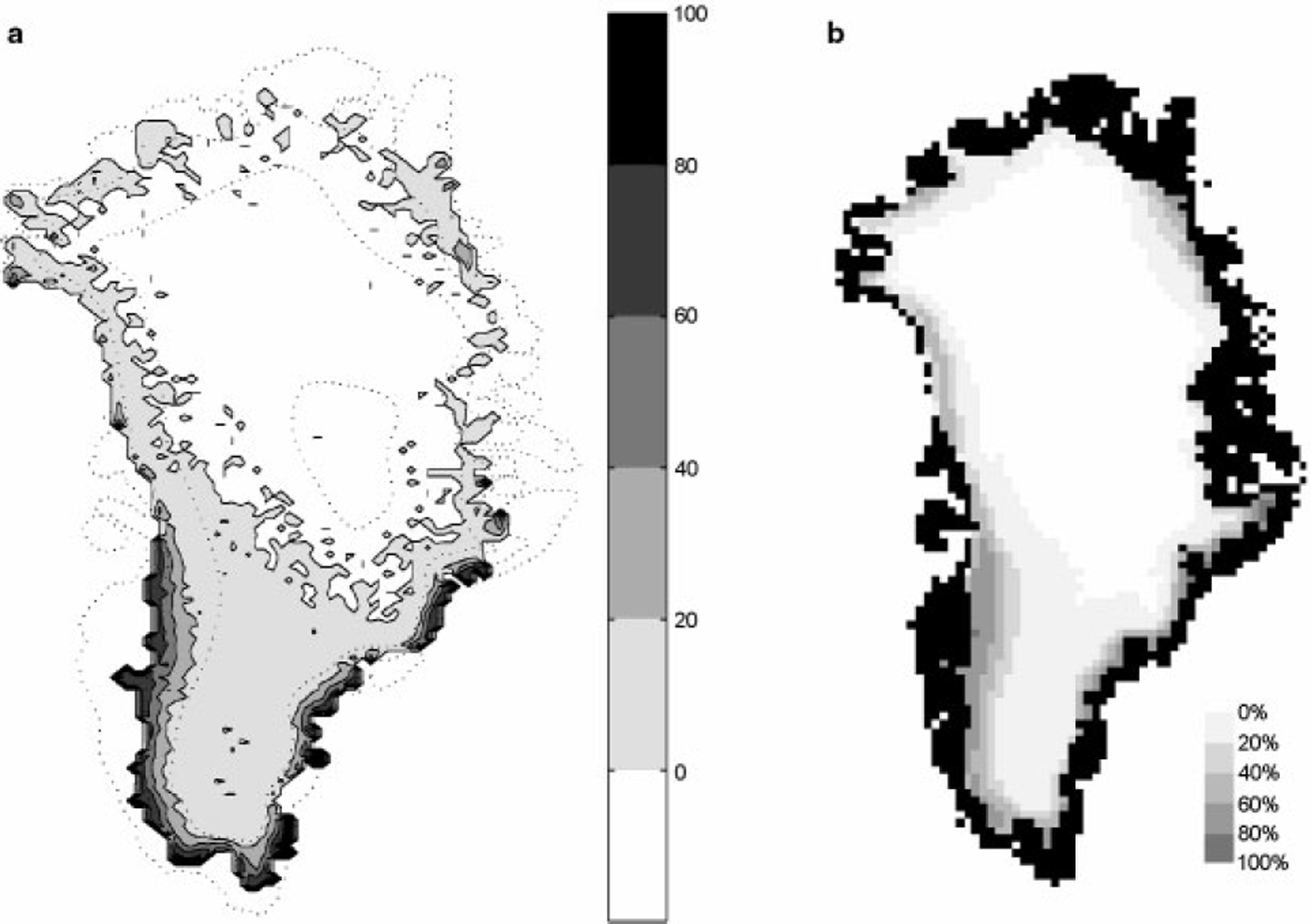
Fig. 1. Extent of the melt zone during the three summer months (June-August). The shading represents the percentage of days which experienced melting during the summer, (a) Derived with the snowPack model; dotted lines are the 1000 m topographic height contours, (b) Satellite microwave remote-sensing observations (Reference Abdalati and StefFenAbdalati and Steffen, 1997).
3.1.3. Ablation on the Greenland ice sheet
The total runoff originating from the Greenland ice sheet calculated by the three melt models is 299, 172 and 162 GTa–1 for the linear, positive degree-day and snowpack models, respectively. The estimates, derived from observations, cited by the Intergovernmental Panel on Climate Change (IPCC) report (1995) are around 237 GTa–1; the measurements are themselves highly uncertain. The values estimated by the snowpack and the PDD model combinations are close and 25–30% lower than the observed value; the linear model predicts significantly more runoff than the snowpack model, and 25% more than observed. Because the snow-cover model underestimates the intensity of melting along the northern coast, 162 GTa–1 is likely to be less than the actual runoff.
3.2. Changes over the 20th century
3.2.1. Climate-model runs
The MIT 2D-LO model was used to simulate a range of transient climate-change scenarios in order to assess how various assumptions in the climate model affect the estimate of sea-level change (Reference Forest, Allen, Stone and SokolovForest and others, 2000). All model runs are forced from 1860 to 1995 with observed changes in greenhouse gases, anthropogenic aerosol and stratospheric ozone concentrations. Two parameters thought a priori to be important in determining the evolution of the model climate are varied within reasonable bounds. The model’s climate sensitivity, S, is varied from 0.7° to 6.2°C by tuning a cloud feedback parameter. The global-mean vertical heat diffusivity, Kv, determines the rate at which heat from the mixed layer penetrates into the deep ocean. Larger diffus-ivities lead to a slower rate of response of the atmosphere to a change in forcing. The range of global-mean vertical diffusivities used is 0.16–40 cm2 s–1. This heat-diffusion coefficient is, however, only a simplifying representation of the role of oceanic convection.
An optimal fingerprint detection technique (Forest and others, in press, and references therein) is used to compare the simulated pattern of climate change with observations. The fingerprint used in this study is the latitude-height pattern of temperature change between the 1961–80 and 1986–95 period means. None of the six runs can be rejected at the 90% confidence level.
3.2.2. Changes in mass balance and sea level
The changes in sea level from 1900 to 1995 are shown in Figure 2. The maximum increase in sea level, –4.5mm, is obtained for the scenario with S = 4.5°C, Kv = 2.5 cm2 s–1. The runs with the largest climate sensitivity and the lowest heat diffusivity exhibit the largest increase in runoff, in particular over the last 50 years of the integration. Accumulation also begins to increase significantly after 1960.
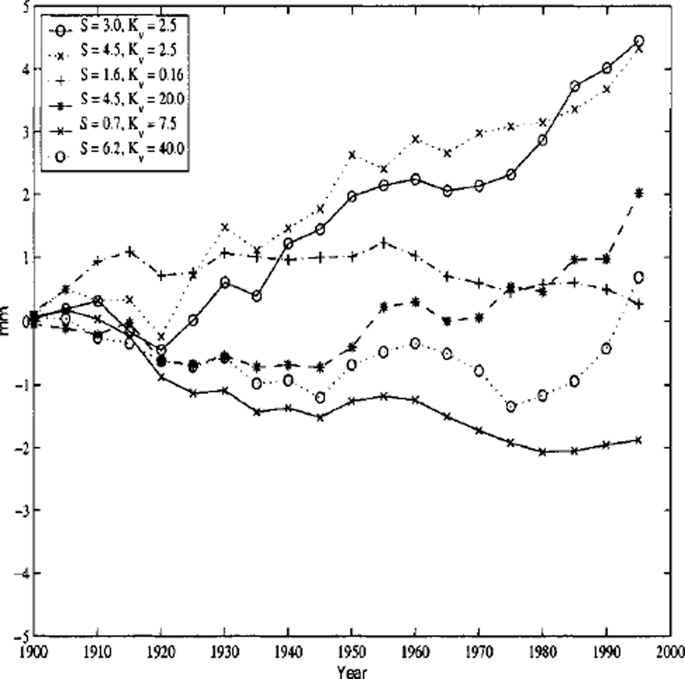
Fig. 2. Sea-level change due to changes in the mass balance of the Greenland ice sheet, 1900–95. All runs are forced by observed changes in atmospheric concentrations of greenhouse gases and anthropogenic aerosols. They differ in their climate sensitivity, S, in °C, and the ocean heat diffusivity, Kv, in cm2 s–1
Conversely, runs with a low climate sensitivity and a high heat diffusivity do not show any significant change in accumulation or runoff from the Greenland ice sheet over the 20th century. The run with S = 0.7°C, Kv = 7.5 cm2 s–1 even shows a slight decrease of 2 mm in the level of the oceans by 1995.
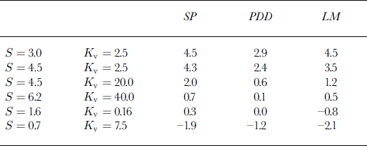
The results obtained with the linear and degree-day models are summarized in Table 1. The linear model reproduces well the changes in mass balance predicted by the snowpack model, indicating that the model is a good approximation for small perturbations around the current climate. The degree-day model predicts significantly less increase in runoff and sea-level changes smaller by 30–40% than the other two models.
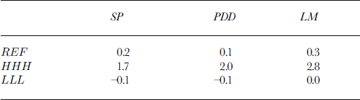
Table 1. Sea-level change ( mm), 1900–95, for six climate-model runs. Estimates of the snowpack (SP), PDD and linear (LM) models. Units of climate sensitivity S are a C; the heat diffusity Kvis in cm2 s–1
3.3. Changes over the 21st century
3.3.1. Climate-change scenarios
The scenarios used over the 21st century are characterized by a three-letter code (Reference PrinnPrinn and others, 1998). The first letter indicates a high, standard or low estimate for the increase in emissions of greenhouse gases. The second letter indicates the rate of warming: lower/higher estimates than the reference value for the aerosol optical depth and the ocean’s heat diffusivity give a rate of warming that is faster/slower than for the reference case. The third letter indicates the sensitivity of the model to greenhouse forcing. The scenarios are considered as equally probable. The HHH scenario combines high emissions, a strong rate of warming and a large climate sensitivity, and has the largest warming of the runs, globally +5.5°C by 2100. The LLL scenario has the smallest warming, +1°C by 2100. The reference scenario, which mimics the IPCC’s IS92a scenario, has a global average increase in temperature of +2.5°C by 2100. The warming predicted for the Arctic is, however, always larger than the global average because of the ice-albedo feedback effect.
3.3.2 Changes in mass balance and sea level
The evolution of accumulation, rainfall, melting, freezing and runoff estimated by the snowpack model between the first and last decade of the REF, HHH and LLL integrations is summarized inTable 2.
Table 2. Evolution of accumulation (snowfall minus evaporation), rainfall, melting, freezing and runoff between the first (1990–2000) and last (2090–2100) decade of the integrations for the REF, HHH and LLL scenarios. Units are 1012kg a–1 = GTa–1 and (mm w.e.)
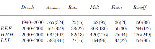
Snow- and rainfall increase steadily over the 21st century, and the rate of increase is clearly linked to rate of warming of the atmosphere. This does not, however, imply that temperature changes control the increase in precipitation; the latter is determined by modifications in atmospheric circulation which accompany the changes in temperature. The capacity of the snow cover to refreeze melt- and rainwater has an important impact on the mass balance; it represents ― 2 0% of the input of liquid water at the beginning of the runs. This capacity does, however, begin to reach saturation as the warming accelerates and more water is added to the snow cover, refreezing drops to ― 15% of melt- and rainwater input by 2100 in the REF and HHH runs. This evolution is linked to changes in the density structure of the snow cover in the ablation region: once the previous winter’s snow is melted and bare ice is exposed, the ability to refreeze water is lost until new snow is deposited.
The estimates of runoff obtained with the temperature-based models for Greenland were within a reasonable range of observations for the current climate. It is therefore particularly interesting to see how they respond to the range of forcing provided by the climate-change scenarios. The changes in sea level by 2100 are summarized in Table 3. There is generally a good agreement between the models over a broad range of forcing. Differences which point to a limitation of the temperature-based methods do, however, begin to appear during the last 20–30 years of the HHH integration. Once ice outcrops during the ablation season, increasing temperatures no longer have much impact on the rate of meltwater formation in the snowpack model; since the albedo of ice is set to a constant value, they contribute only to an expansion of the melt zone. The amount of runoff predicted by the degree-day and linear models does, however, continue to increase linearly with temperature.
Table 3. Sea-level change (cm) associated with the REF, HHH, LLL scenarios and the three snowmelt models
The increase in accumulation is balanced by the increase in runoff in Greenland for the REF run, and the net sea-level change is very small. This is to a certain extent also the case for the other six scenarios, shown in Figure 3. The +1.8 cm increase in sea level associated with the HHH scenario is the result of a 4.2 cm rise due to increased runoff and of a 2.6 cm drop associated with increased accumulation. The absence of large changes in sea level gives the false impression that the mass balance of the Greenland ice sheet is relatively insensitive to changes in climate, when in fact the amount of meltwater runoff has doubled or tripled by 2100.
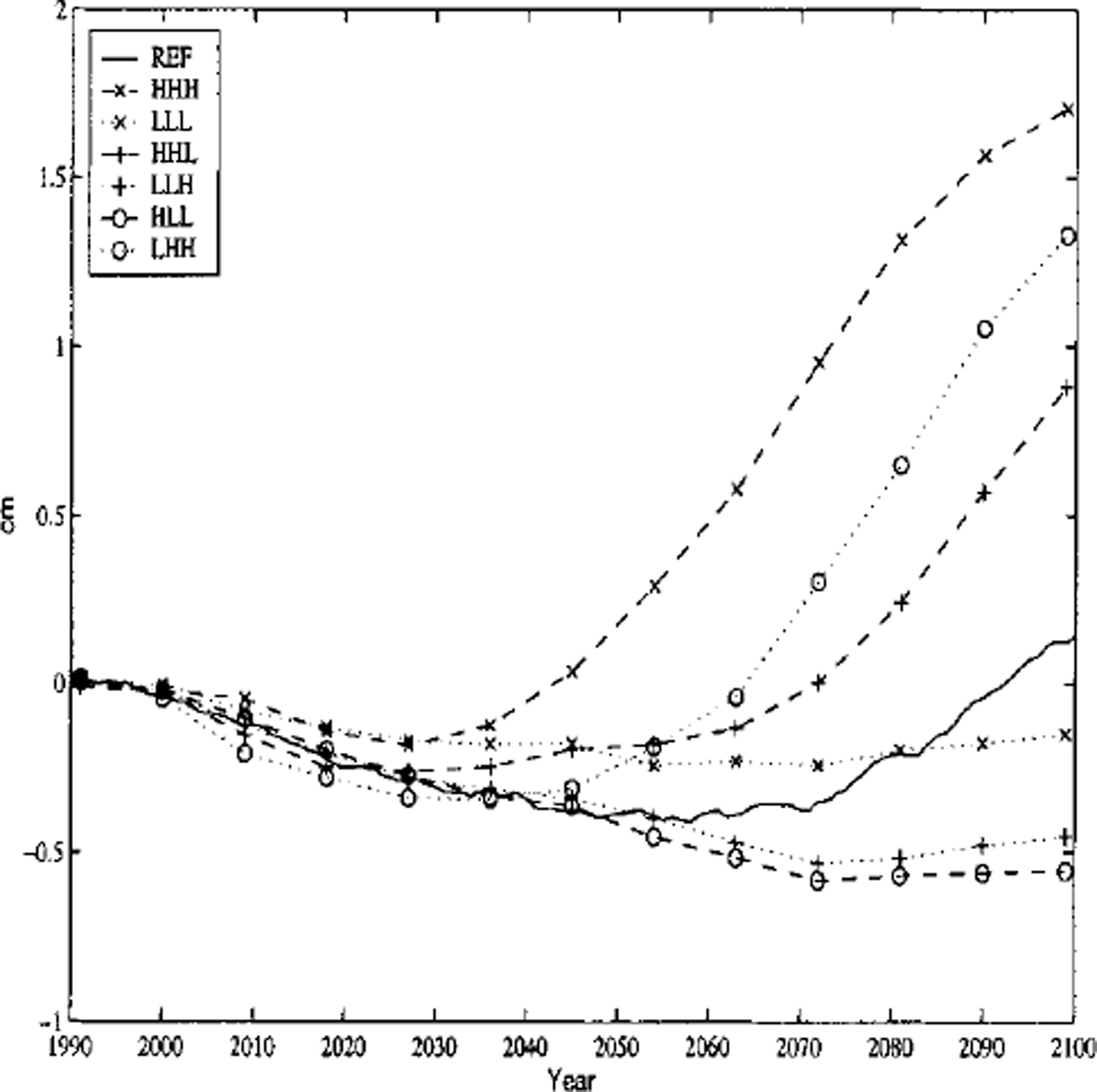
Fig. 3. Sea-level change due to changes in the mass balance of the Greenland ice sheet, 1990–2100, for seven climate-change scenarios.
The most important factor in determining the range of uncertainty in the estimates of sea-level rise is not the rate of increase in emissions of greenhouse gases, but the rate at which heat diffuses into the ocean and delays the warming of the atmosphere. The scenarios which have a low ocean diffusivity (middle letter H) end up with a larger sea-level rise than those with high ocean diffusivities (middle letter L).
4. Conclusion
The results obtained with the snow-cover model have more credibility than those derived with simple parameterization, in part because it is the surface energy balance and not the air temperature which drives the melting process, but also because the amount of meltwater which refreezes in the firn depends on the local density and temperature structure within the snow cover. The parameterization of snow and ice albedo in the snowpack model has a strong influence on the results; reducing the uncertainty in this and other aspects of the model is an important objective.
Temperature-based methods such as the degree-day and linear models are calibrated to the range of temperatures and conditions observed currently in southern Greenland. The results obtained over the 20th century indicate that the linear model performs well for small changes in forcing, less so when temperatures increase beyond what is currently observed (e.g. in the HHH scenario). The degree-day model is less sensitive to small temperature changes than the other two models, but performs well for larger changes in forcing.
The changes in sea level estimated by all three models for the 20th and 21st centuries cannot be distinguished from zero at any confidence level. Because increases in accumulation tend to offset increases in runoff, the range of uncertainty is fairly small, 0.6 cm for the 20th century, 2.2 cm by 2100 for the snowpack model.
In order to avoid excessive computation requirements, simplifications in the climate models are, however, required to perform transient simulations, in particular the multiple integrations needed to quantify the uncertainty of the predictions. The weakness of this study lies in the inability of the MIT climate model to capture regional climate changes, for example in the location and intensity of the Atlantic storm track, or changes in the intensity of the thermohaline circulation, which would have an impact on the mass balance of the Greenland ice cap. The zonal model is, however, designed to capture global-scale changes in the atmospheric circulation and in the moisture transport.
Acknowledgements
This research was supported by the Alliance for Global Sustainability, the MIT Joint Program on the the Science and Policy of Global Change and NASA grant NAG 5–7204 as part of the NASA GISS Interdisciplinary Earth Observing System Investigation.


