


1. Introduction
Understanding the behaviour of dispersed particles in turbulent flows is relevant in many contexts. In modelling oil spills, knowledge of the oil droplet dispersion characteristics is important in determining their transport (North et al. Reference North, Adams, Thessen, Schlag, He, Socolofsky, Masutani and Peckham2015; Yang et al. Reference Yang, Chen, Socolofsky, Chamecki and Meneveau2016). The oil slicks are broken down into polydisperse droplet distributions that are transported by waves and turbulence. The smaller droplets are more horizontally dispersed by the turbulence, while the larger ones rise towards the surface. In studying disease transmission, the dispersion characteristics and size distribution of particles ejected from a sneeze or cough affect their residence time and transport properties in the air, information necessary to formulate social distancing and masking rules (Bourouiba Reference Bourouiba2020; Mittal, Ni & Seo Reference Mittal, Ni and Seo2020). There have been considerable efforts in studying dispersion of bubbles and heavy particles in turbulence (Corrsin & Lumley Reference Corrsin and Lumley1956; Csanady Reference Csanady1963; Snyder & Lumley Reference Snyder and Lumley1971; Reeks Reference Reeks1977; Wells & Stock Reference Wells and Stock1983; Wang & Stock Reference Wang and Stock1992; Stout, Arya & Genikhovich Reference Stout, Arya and Genikhovich1995; Kennedy & Moody Reference Kennedy and Moody1998; Mazzitelli & Lohse Reference Mazzitelli and Lohse2004). Polydispersity adds an additional layer of complexity in characterizing particle dispersion due to the interplay of inertial effects (lift forces on different sized particles) and buoyancy effects that can affect particles of different sizes quite differently. The particle–turbulence interactions result in interesting phenomena such as preferential concentration (Squires & Eaton Reference Squires and Eaton1991; Eaton & Fessler Reference Eaton and Fessler1994), particle clustering (Obligado et al. Reference Obligado, Teitelbaum, Cartellier, Mininni and Bourgoin2014; Falkinhoff et al. Reference Falkinhoff, Obligado, Bourgoin and Mininni2020) (either strain or vorticity dominated) and modified turbulent diffusion due to particle trajectory crossing (Yudine Reference Yudine1959; Csanady Reference Csanady1963; Wells & Stock Reference Wells and Stock1983). This effect refers to the relative motion between particles and turbulent eddies in the continuous phase.
Yudine (Reference Yudine1959) and Csanady (Reference Csanady1963) studied the case of finite particle rise velocity and zero particle inertia. The velocity correlation seen by the heavy particle  $\langle u^{p}_i(0)\,u^{p}_j(\tau )\rangle$ can be approximated by the Eulerian spatial velocity correlation of the flow $\langle u_i(\boldsymbol {x_0},t_0)\,u_j(\boldsymbol {x_0} + \boldsymbol{W}_{r}\tau,t_0)\rangle$ for small particle correlation time $\tau$, where $u_i(\boldsymbol {x},t)$ is the $i$th component of the fluid Eulerian velocity. The effect of the rise velocity $W_r$ on the velocity correlation was termed the ‘crossing-trajectories effect’. Csanady (Reference Csanady1963) found that the effect of increasing finite rise/free fall velocity was to reduce both the transverse and longitudinal (with respect to the free fall direction) dispersion coefficients. Wang & Stock (Reference Wang and Stock1992) presented a comprehensive analysis for the dispersion coefficients of heavy particles in isotropic turbulence by separating the effects of inertia and particle rise velocity. They defined a non-dimensional inertia parameter (based on the particle Stokes number) and a rise parameter (based on the rise/fall velocity) to characterize the dispersion of heavy particles. Particles dispersed faster than the fluid elements if the inertia parameter controlled the dispersion (large Stokes number), and slower than the fluid elements if the drift parameter governed the dispersion. The finite free fall (or rise) velocity of particles causes them to migrate out of eddies before they decay (Yudine Reference Yudine1959). This results in particles losing their velocity correlation more rapidly than fluid elements. The particle dispersion is thereby reduced as the particle correlation times are directly related to their dispersion coefficient (Taylor Reference Taylor1922). The following relations were obtained for the normalized particle dispersion coefficients by Wells & Stock (Reference Wells and Stock1983):
 \begin{gather} \frac{D_{p,L}}{D_{f,L}} = \left(1 + \frac{C W_{r}^{2}}{w^{'2}}\right)^{{-}1/2}, \end{gather}
 \begin{gather}\frac{D_{p,T}}{D_{f,T}} = \left(1 + \frac{4C W_{r}^{2}}{w^{'2}}\right)^{{-}1/2}, \end{gather}
where  $D_{p,L}$, $D_{f,L}$, $D_{p,T}$, $D_{f,T}$ are the longitudinal and transverse particle and fluid dispersion coefficients, respectively, $W_{r}$ is the particle rise velocity (in the vertical direction), $C = w' T_L/L_E$ relates the Lagrangian timescale $T_L$ to the Eulerian length scale $L_E$, and $w'$ is the axial turbulent fluctuation velocity (in the direction of the rise velocity). Note that the crossing trajectory effect referred to here is the one defined by Yudine (Reference Yudine1959) that accounts for the effect of a finite drift velocity on the velocity fluctuations to be distinguished from the different effect of multivalued particle velocity at a given space–time instant (Laurent et al. Reference Laurent, Vié, Chalons, Fox and Massot2012).
A number of experimental studies have focused on oil droplets in water, i.e. cases where particles are only slightly buoyant. For instance, Friedman & Katz (Reference Friedman and Katz2002) have shown that the rise velocities and dispersion characteristics of slightly buoyant oil-in-water droplets differ significantly from those of bubbles and heavy particles. Gopalan, Malkiel & Katz (Reference Gopalan, Malkiel and Katz2008) studied the dispersion characteristics of oil droplets in water experimentally in isotropic turbulence. They calculated the turbulent diffusion coefficient by integrating the ensemble-averaged Lagrangian velocity autocovariance and found a dependence of the diffusion coefficient on the ratio of the turbulence intensity and the droplet rise velocity.
Besides experiments, recent years have seen a significant number of computer simulation based studies of particle-laden turbulent flows. Numerical approaches for the particle phase can be classified broadly into either Lagrangian models, where individual droplets or droplet clusters are tracked in Lagrangian fashion, or Eulerian models, where the distribution of particles is treated as a continuous density field (Balachandar & Eaton Reference Balachandar and Eaton2010; Fox Reference Fox2011; Subramaniam Reference Subramaniam2013). Direct numerical simulations (DNS) of the continuous phase coupled with a Lagrangian approach for the particles provide the highest fidelity, but often have a prohibitively high computational cost due to the large number of particles that need to be tracked and resolved, in addition to the high cost of having to resolve the continuous phase down to the Kolmogorov scale. Large eddy simulations (LES), on the other hand, capture the large- and intermediate-scale turbulent motions (based on the grid resolution), and require only modelling of the unresolved subgrid-scale (SGS) turbulence effects. While the cost of LES is higher than Reynolds-averaged Navier–Stokes (RANS) simulations, LES provide the ability to resolve unsteady spatially fluctuating phenomena at least down to scales of the order of the grid scale. The conventional wisdom is that turbulent transport is dominated by the largest eddies in the flow, therefore LES neglecting SGS effects other than the SGS eddy diffusivity should provide robust and accurate predictions in general. However, the direct effect of the SGS velocity has already been shown to be important for particle clustering, preferential concentration and particle statistics, particularly for small particle time scale (or Stokes number) when the grid resolution of LES is coarse (Armenio, Piomelli & Fiorotto Reference Armenio, Piomelli and Fiorotto1999; Marchioli Reference Marchioli2017). In order to account for the SGS fluid field on the particle evolution, numerous models have been developed, such as those based on approximate-deconvolution methods (Stolz, Adams & Kleiser Reference Stolz, Adams and Kleiser2001; Shotorban & Mashayek Reference Shotorban and Mashayek2005) or Lagrangian stochastic models (Mazzitelli & Lohse Reference Mazzitelli and Lohse2004; Minier, Peirano & Chibbaro Reference Minier, Peirano and Chibbaro2004; Oesterlé & Zaichik Reference Oesterlé and Zaichik2004; Shotorban & Mashayek Reference Shotorban and Mashayek2006; Johnson & Meneveau Reference Johnson and Meneveau2018; Knorps & Pozorski Reference Knorps and Pozorski2021). These models aim to describe the unresolved portions of the fluid velocity as seen by the particle. These models include various terms in their parameterization to capture the effect of crossing trajectories, particle inertia, flow anisotropy, etc. (Berrouk et al. Reference Berrouk, Laurence, Riley and Stock2007; Michałek et al. Reference Michałek, Kuerten, Liew, Zeegers and Geurts2013). The models are developed for cases where the particle phase is modelled using a Lagrangian approach, with the velocity field modelled using an Eulerian model.
There have been efforts in modelling the crossing trajectory effect for particles in homogeneous isotropic turbulence and shear flows in the presence of an external force field. Simonin, Deutsch & Minier (Reference Simonin, Deutsch and Minier1993) developed a closure equation for the fluid/particle moments required for dispersed phase modelling in the framework of a two-fluid model. Pozorski & Minier (Reference Pozorski and Minier1998) modelled the crossing trajectory effect by introducing a Langevin model for the mean drift velocity. Moment-based methods have also been used by Salehi et al. (Reference Salehi, Cleary, Masri and Kronenburg2019) to study polydisperse inertial particles. Oesterlé (Reference Oesterlé2009) provided an alternative theoretical analysis of the time correlation of the fluid velocity fluctuations using Langevin-type stochastic models to predict the effects of crossing trajectories in shear flows. Using DNS with Lagrangian modelling of heavy particles, Fede & Simonin (Reference Fede and Simonin2006) have quantified the effects of the particle trajectory crossing effect on the structure of SGS turbulence and its time scales.
For applications with relatively low volume fractions and low particle Stokes number, Eulerian approaches for the particle field can be advantageous as they are not limited by the number of particles (Fox, Laurent & Massot Reference Fox, Laurent and Massot2008; Laurent et al. Reference Laurent, Vié, Chalons, Fox and Massot2012; Masi et al. Reference Masi, Simonin, Riber, Sierra and Gicquel2014; Vié et al. Reference Vié, Pouransari, Zamansky and Mani2016). Pandya & Mashayek (Reference Pandya and Mashayek2002) and Zaichik, Simonin & Alipchenkov (Reference Zaichik, Simonin and Alipchenkov2009) formulated a two-fluid LES approach for particle-laden turbulent flows. The approach was based on a kinetic equation for the filtered probability density of the particle velocity, and was valid for larger Stokes numbers. In the equilibrium Eulerian approach (Ferry & Balachandar Reference Ferry and Balachandar2001; Shotorban & Balachandar Reference Shotorban and Balachandar2007, Reference Shotorban and Balachandar2009), the particle velocities are modelled as a function of the particle time scale to include effects of buoyancy, added mass and SGS effects. The particles are represented by a continuous concentration field, and a separate transport equation is solved for each particle size (Yang et al. Reference Yang, Chen, Socolofsky, Chamecki and Meneveau2016; Aiyer et al. Reference Aiyer, Yang, Chamecki and Meneveau2019). The LES of polydisperse droplets/bubbles with the equilibrium Eulerian approach have been used to study bubble driven plumes by Yang et al. (Reference Yang, Chen, Socolofsky, Chamecki and Meneveau2016) and have been coupled with population balance equations to model droplet breakup by Aiyer et al. (Reference Aiyer, Yang, Chamecki and Meneveau2019) and Aiyer & Meneveau (Reference Aiyer and Meneveau2020). Due to its advantages for LES of low-volume-fraction oil–water multiphase flows where the particle Stokes number is small, in this paper we focus on the equilibrium Eulerian model. Specifically, we aim to explore the degree to which the approach is able to capture effects of particle trajectory crossing, and whether for LES performed at very coarse resolutions, additional required subgrid modelling can be developed.
The paper begins in § 2 by describing the Eulerian–Eulerian LES approach. In § 3, we present results from well-resolved LES of a turbulent jet with droplets injected at the source of the jet. Results motivate the development of a modified Schmidt number subgrid model to account for crossing trajectory effects. Implementation and validation of the proposed modified subgrid turbulent diffusion model are presented in § 4. Conclusions are presented in § 5
2. Equilibrium Eulerian large eddy simulation
2.1. Governing equations and numerical methods
Let  $\boldsymbol {x} {} = (x,y,z)$, with $x$ and $y$ the horizontal coordinates, and $z$ the vertical direction, and let $u {} = (u,v,w)$ be the corresponding velocity components. Also, $n_i$ is the number density of a droplet of size $d_i$. The jet and surrounding fluid are governed by the three-dimensional incompressible filtered Navier–Stokes equations with a Boussinesq approximation for buoyancy effects, while the droplet concentration fields are governed by Eulerian transport equations at each size:
 \begin{gather}
\boldsymbol{\nabla}\boldsymbol{\cdot}
\boldsymbol{\tilde{u}} =0, \end{gather}
\begin{gather}
\boldsymbol{\nabla}\boldsymbol{\cdot}
\boldsymbol{\tilde{u}} =0, \end{gather}
 \begin{gather}\frac{\partial \boldsymbol{\tilde{u}}}{\partial
t} + \boldsymbol{\tilde{u}}\boldsymbol{\cdot}\boldsymbol{\nabla}\boldsymbol{\tilde{u}}={-}\frac{1}{\rho_c} \boldsymbol{\nabla}\tilde{P}{} -
\boldsymbol{\nabla}\boldsymbol{\cdot}\boldsymbol{\tau}
{}^{d} +\tilde{F}\,\boldsymbol{e} {}_3
+\left(1-\frac{\rho_d}{\rho_c}\right)\sum_i(V_{d,i}\tilde{n}
{}_i)g\,\boldsymbol{e} {}_3,
\end{gather}
\begin{gather}\frac{\partial \boldsymbol{\tilde{u}}}{\partial
t} + \boldsymbol{\tilde{u}}\boldsymbol{\cdot}\boldsymbol{\nabla}\boldsymbol{\tilde{u}}={-}\frac{1}{\rho_c} \boldsymbol{\nabla}\tilde{P}{} -
\boldsymbol{\nabla}\boldsymbol{\cdot}\boldsymbol{\tau}
{}^{d} +\tilde{F}\,\boldsymbol{e} {}_3
+\left(1-\frac{\rho_d}{\rho_c}\right)\sum_i(V_{d,i}\tilde{n}
{}_i)g\,\boldsymbol{e} {}_3,
\end{gather}
 \begin{gather}\frac{\partial \tilde{n}
{}_i}{\partial t} + \boldsymbol{\nabla}\boldsymbol{\cdot}
(\boldsymbol{\tilde{V}}{}_i\tilde{n} {}_i) + \boldsymbol{\nabla}\boldsymbol{\cdot}
\boldsymbol{\rm \pi}_{i} = \tilde{q}_{i},\quad i=1, 2,\ldots,N.
\end{gather}
\begin{gather}\frac{\partial \tilde{n}
{}_i}{\partial t} + \boldsymbol{\nabla}\boldsymbol{\cdot}
(\boldsymbol{\tilde{V}}{}_i\tilde{n} {}_i) + \boldsymbol{\nabla}\boldsymbol{\cdot}
\boldsymbol{\rm \pi}_{i} = \tilde{q}_{i},\quad i=1, 2,\ldots,N.
\end{gather}
A tilde denotes a variable resolved on the LES grid,  $\boldsymbol{\tilde{u}}$ is the filtered fluid velocity, $\rho _d$ is the density of the droplet, $\rho _c$ is the carrier fluid density, $V_{d,i}={\rm \pi} d_i^{3}/6$ is the volume of a spherical droplet of diameter $d_i$, $\boldsymbol {\tau } = (\boldsymbol{\widetilde{uu}}-\boldsymbol{\tilde{u}}\boldsymbol{\tilde{u}})$ is the SGS stress tensor (superscript ‘ $d$’ denotes its deviatoric part), $\tilde {n} {}_i$ is the resolved number density of the droplet of size $d_i$, $\tilde {F}$ is a locally acting upward body force to simulate the jet momentum injection, and $\boldsymbol {e} {}_3$ is the unit vector in the vertical direction. The droplet Eulerian description has been used previously to study monodisperse plumes (Yang, Chamecki & Meneveau Reference Yang, Chamecki and Meneveau2014; Yang et al. Reference Yang, Chen, Chamecki and Meneveau2015; Chen et al. Reference Chen, Yang, Meneveau and Chamecki2016; Yang et al. Reference Yang, Chen, Socolofsky, Chamecki and Meneveau2016) and polydisperse oil plumes (Aiyer et al. Reference Aiyer, Yang, Chamecki and Meneveau2019; Aiyer & Meneveau Reference Aiyer and Meneveau2020). The filtered version of the transport equation for the number density $\tilde {n}_i(\boldsymbol {x} {},t;d_i)$ is given by (2.3). The term $\boldsymbol{\rm \pi} _{i} = (\widetilde{\boldsymbol{V}{}_{i}n_{i}}- \boldsymbol{\tilde{V}}_{i}\tilde{n_{i}})$ is the SGS concentration flux of oil droplets of size $d_i$ (no summation over $i$ is implied here), and $\tilde {q}_i$ denotes the injection rate of droplets of diameter $d_i$. In order to capture a range of sizes, the number density distribution function is discretized into $N$ linearly distributed bins, and we solve $N$ separate transport equations for the number densities $\tilde {n}_i(\boldsymbol {x} {},t;d_i)$ with $i=1,2,\ldots,N$.
Closure for the SGS stress tensor  $\boldsymbol {\tau } {}^{d}$ is obtained from the Lilly–Smagorinsky eddy viscosity model, with a Smagorinsky coefficient $c_s$ determined dynamically during the simulation using the Lagrangian averaging scale-dependent dynamic (LASD) SGS model (Bou-Zeid, Meneveau & Parlange Reference Bou-Zeid, Meneveau and Parlange2005). In the current simulations, the viscous stress contribution has been neglected. The eddy viscosity at the centreline of the jet for the configurations considered here is ${\sim }20$ times the molecular viscosity. Towards the edge of the jet at $r/r_{1/2} = 2$, the value decays to 10 times the molecular viscosity. The viscous stress would be important in the near nozzle region of the jet, a region not included explicitly in the present LES. The SGS scalar flux ${\rm \pi} _{i}$ is modelled using an eddy diffusion SGS model. We follow the approach of Yang et al. (Reference Yang, Chen, Socolofsky, Chamecki and Meneveau2016) and prescribe a constant turbulent Schmidt/Prandtl number, $Pr_{sgs} = Sc_{sgs} =0.4$. The SGS flux is thus parameterized as $\boldsymbol{\rm \pi} _{n,i} = -(\nu _{sgs}/Sc_{sgs})\,\boldsymbol {\nabla }\tilde {n} {}_{i}$. With the evolution of oil droplet concentrations being simulated, their effects on the fluid velocity field are modelled and implemented in (2.2) as a buoyancy force term (the last term on the right-hand side of the equation) using the Boussinesq approximation. A basic assumption for treating the oil droplets as a Boussinesq active scalar field being dispersed by the fluid motion is that the volume and mass fractions of the oil droplets are small within a computational grid cell. The droplet transport velocity $\boldsymbol{\tilde {V}}_i$ is calculated by an expansion in the droplet time scale $\tau _{d,i}=(\rho _d+\rho _c/2)d_i^{2}/(18\mu _f)$ (Ferry & Balachandar Reference Ferry and Balachandar2001). The expansion is valid when $\tau _{d,i}$ is much smaller than the resolved fluid time scales, which requires us to have a grid Stokes number $St_{\varDelta,i} = \tau _{d,i}/\tau _{\varDelta } \ll 1$, where $\tau _{\varDelta }$ is the turbulent eddy turnover time at scale $\varDelta$. The transport velocity $\boldsymbol{\tilde {V}}_i$ of droplets of size $d_i$ is given by (Ferry & Balachandar Reference Ferry and Balachandar2001)
 \begin{equation} \boldsymbol{\tilde{V}}_i = \boldsymbol{\tilde{u}} + W_{r,d_i}\,\boldsymbol{e} {}_3 + (R-1)\tau_{d,i}\left(\frac{D\boldsymbol{\tilde{u}}}{D t} + \boldsymbol{\nabla}\boldsymbol{\cdot}\boldsymbol{\tau} {}\right), \end{equation}
where  $\boldsymbol {e} {}_3$ is the unit vector in the vertical direction, and $R = 3\rho _c/(2\rho _{d}+\rho _c)$ is the acceleration parameter. The droplet rise velocity is calculated as a balance between the drag and buoyancy force acting on a droplet:
 \begin{equation} W_{r,d_i} = \begin{cases} W_{r,S}, & \text{if}\ Re_i < 0.2, \\ W_{r,S}(1+0.15Re_i^{0.687})^{{-}1}, & 0.2 < Re_i< 750, \end{cases} \end{equation}
where
 \begin{equation} W_{r,S} = \frac{(\rho_c-\rho_d)g d_i^{2}}{18\mu_f}, \end{equation} $Re_i = \rho _c W_{r,d_i} d_i/\mu _c$ is the droplet rise velocity Reynolds number, and $g=9.81\ \mathrm {m}\ \mathrm {s}^{-2}$ is the gravitational acceleration. The effects of drag, buoyancy, added mass and the divergence of the subgrid stress tensor have been included in the droplet velocity expansion. A more detailed discussion of the droplet rise velocity in (2.4) can be found in Yang et al. (Reference Yang, Chen, Socolofsky, Chamecki and Meneveau2016). While in general an additional term proportional to the difference of particle and local fluid accelerations should be included (Climent & Magnaudet Reference Climent and Magnaudet1999), Bec et al. (Reference Bec, Biferale, Boffetta, Celani, Cencini, Lanotte, Musacchio and Toschi2006) showed that for Stokes number $St < 0.4$, the difference between the rate of variation of particle momentum and the rate of variation of the fluid momentum at the particle position can be neglected.
Equations (2.1) and (2.2) are discretized using a pseudo-spectral method on a collocated grid in the horizontal directions and a centred finite difference scheme on a staggered grid in the vertical direction (Albertson & Parlange Reference Albertson and Parlange1999). Periodic boundary conditions are applied in the horizontal directions for the velocity and pressure fields. The transport equations for the droplet number densities, (2.3), are discretized as in Chamecki, Meneveau & Parlange (Reference Chamecki, Meneveau and Parlange2008), by a finite-volume algorithm with a bounded third-order upwind scheme for the advection term. A fractional-step method with a second-order Adams–Bashforth scheme is applied for the time integration, combined with a standard projection method to enforce the incompressibility constraint. The same methods were used in Yang et al. (Reference Yang, Chen, Socolofsky, Chamecki and Meneveau2016) and Aiyer et al. (Reference Aiyer, Yang, Chamecki and Meneveau2019), where more detailed descriptions can be found.
2.2. Simulation set-up
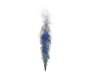
The injected jet is modelled in the LES using a locally applied vertically upward pointing body force following the procedure outlined in Aiyer et al. (Reference Aiyer, Yang, Chamecki and Meneveau2019) and Aiyer (Reference Aiyer2020). We use this approach since at the LES resolution used in the current applications it is not possible to resolve the small-scale features of the injection nozzle. A sketch for the simulation set-up is shown in figure 1. The body force is applied downstream of the true nozzle ( $D_J$ in figure 1) at a location $z = 10 D_J$, where the actual jet being modelled would have grown for the LES grid resolution to be sufficient to resolve its large-scale features. The strength of the body force is specified so as to obtain an injection velocity of $2\ {\rm m}\ {\rm s}^{-1}$. Random fluctuations are added to the horizontal components of the momentum equation to induce transition to turbulence. The fluctuations have an amplitude with a root-mean-square value equal to 0.1 % of the magnitude of the forcing $\tilde {F}$, and are applied only during an initial period of 0.5 s at the forcing source. The forcing is applied only over a finite volume and smoothed using a super-Gaussian kernel. A summary of important simulation parameters is provided in table 1. The first set of simulations uses a relatively fine grid with $N_x \times N_y\times N_z = 288 \times 288 \times 384$ points for spatial discretization, and a time step $\Delta t = 3 \times 10^{-4}$ s for time integration. The resolution in the horizontal directions, $\Delta x = \Delta y = 3.47$ mm is set to ensure that at the location where the LES begin to resolve the jet, we have at least three points across the jet. In the vertical direction, we use a grid spacing of $\Delta z = 6.5$ mm, enabling us to capture a domain height 2.5 times the horizontal domain size. This configuration has been validated with DNS data and shown to be robust in producing realistic turbulent round jet statistics (Aiyer & Meneveau Reference Aiyer and Meneveau2020).

Figure 1. (a) Sketch of the simulation set-up. Volume rendering of the instantaneous  $50\ \mathrm {\mu }\mbox {m}$ diameter droplet concentration (b) Sketch depicting the LES nozzles ( $D_{LES,1}$, $D_{LES,2}$), the virtual (true) nozzle ( $D_J$) and the droplet injection locations ( $I_1$, $I_2$).
Table 1. Simulation parameters.
The droplets are injected at the source location  $I_1$ (see figure 1), and the droplet number density fields are initialized to zero in the rest of the domain. The initial droplet size distribution is uniform, and the initial droplet velocity is the rise velocity defined in (2.4). In order to avoid additional transient effects, the concentration equations are solved only after a time at which the jet in the velocity field has reached near the top boundary to allow the flow to be established. The number density transport contains a source term $\tilde {q}_i$ on the right-hand side of (2.3) that represents injection of droplets of a particular size. The droplet size range is discretized into $N = 10$ sizes spanning a range from $d_1 = 50\ \mathrm {\mu }{\rm m}$ to $d_{10} = 1\ {\rm mm}$. Droplets of different sizes are injected with a constant source flux $q_i = \tilde {q}_iV_{d,i} = 0.1\ {\rm l}\ {\rm min}^{-1}$ corresponding to a total volume flux $Q_0 = 1\ {\rm l}\ {\rm min}^{-1}$. The source is centred at $(x_c, y_c) = (0.5\ {\rm m}, 0.5\ {\rm m})$ and distributed over two grid points in the $z$ direction with weights $0.7$ and $0.3$ at $z_c$ and $z_{c}+\Delta z$, respectively, and over three grid points in the horizontal directions with weights $0.292$ at $(x_c,y_c)$ and $0.177$ at $(x_{c}\pm \Delta x,y_{c}\pm \Delta y)$. The initial droplet size distribution does not effect the properties of the jet due to the small volume fraction of the dispersed phase (Aiyer & Meneveau Reference Aiyer and Meneveau2020).
3. The LES of droplet transport: size-dependent turbulent diffusion
We first examine instantaneous velocity and concentration contours on the mid- $y$-plane as a function of $x$ and $z$ in figure 2. Figure 2(a) depicts the instantaneous vertical velocity, while figure 2(b) shows the concentration of the $d=50\ \mathrm {\mu }{\rm m}$ droplet and the contour lines of the $d=1000\ \mathrm {\mu }$m-sized droplets. Visually, we can see already that the smallest droplets spatial distribution has a wider horizontal extent as we move further from the injection location as compared to the width of the distribution of larger droplets.

Figure 2. (a) Instantaneous snapshot of the velocity at the midplane of the jet in logarithmic scale; (b) instantaneous concentration contours for  $d= 50\ \mathrm {\mu }{\rm m}$ (colour) and $d = 1\ {\rm mm}$ (lines, contour level $\tilde {c}=10^{-4}$) at the midplane of the jet.
3.1. Mean velocity and concentration profiles
The statistics of the velocity and concentration fields are presented using a cylindrical coordinate system, with  $z$ being the axial coordinate, and supplement the time averaging with additional averaging over the angular $\theta$ direction around the jet axis. The LES data on the Cartesian grid are interpolated using bilinear interpolation onto a much finer $\theta$ grid in the horizontal directions to generate smoother profiles after averaging over the $\theta$ direction.
Results for the radial profiles of the mean velocity and total concentration at various downstream locations are shown in figure 3. We see that the profiles show good collapse when plotted as a function of the scaled coordinate  $r/r_{1/2}$. The LES also show relatively good agreement when compared to DNS data for passive scalars from Lubbers, Brethouwer & Boersma (Reference Lubbers, Brethouwer and Boersma2001). Profiles for the half-width and the vertical velocity for the jet for a similar configuration have been discussed previously in Aiyer & Meneveau (Reference Aiyer and Meneveau2020), and have been omitted here for the sake of brevity.

Figure 3. (a) Axial mean velocity profiles as functions of normalized radial distance; (b) mean total concentration profiles at  $z/D_{J} = 161$ ( $\triangle$, red), $z/D_{J} = 213$ ( $\circ$, green), $z/D_{J} = 252$ ( $\square$, blue) and $z/D_{J} = 342$ ( ${\rhd }, \text {magenta}$) as functions of self-similarity variable $r/r_{1/2}$. The total concentration refers to $\tilde {c} = \sum {\tilde {c}_i}$, where $\tilde {c}_i = \tilde {n}_i ({{\rm \pi} }/{6})d_i^{3}$. The dashed line (- -) denotes the DNS data (Lubbers et al. Reference Lubbers, Brethouwer and Boersma2001).
The profiles of the individual concentration fields are shown in figure 4 for four representative sizes and at different downstream locations. At the location nearest to the nozzle, at  $z/D_J = 108$, we see that there is little difference between the radial profiles for the different droplet sizes. This is in agreement with the qualitative trends seen in the contour plot shown in figure 2. Further downstream, we can see an increasing size dependence in the radial distribution of the concentration field, where the smaller droplet sizes have a wider width as compared to the larger droplets. This observation is consistent with Gopalan et al. (Reference Gopalan, Malkiel and Katz2008) and can be attributed to the increasing ratio of rise velocity to the turbulent axial fluctuating velocity component, $S_v = W_{r,d_i}/w^{\prime }$, where $S_v$ is the settling parameter (Chamecki et al. Reference Chamecki, Chor, Yang and Meneveau2019). The axial and radial profiles of the settling parameter for different droplet sizes are shown in figure 5. When the ratio increases, droplets move from one eddy to another faster than the eddy decay rate. For instance, nearer to the nozzle at $z/D_J = 108$, $W_{r,d_{10}}^{2}/w^{\prime 2} = 0.16$, and the ratio of the transverse particle to the fluid diffusion coefficient can be estimated using (1.1) to be $D_{p,T}/D_{f,T} = 0.8$. Further downstream at $z/D_J = 200$, $W_{r,d_{10}}^{2}/w^{\prime 2} = 0.64$ and $D_{p,T}/D_{f,T} = 0.56$. We can see from figure 5(b) that the ratio also increases as a function of radial distance as the turbulence gets weaker towards the edge of the jet. This results in decreased dispersion for the larger droplets as a function of axial and radial distance.

Figure 4. Normalized radial concentration profiles for different droplet sizes at (a)  $z/D_J =108$, (b) ${z/D_J = 160}$, (c) $z/D_J = 212$ and (d) $z/D_J = 264$. The lines correspond to the individual droplets of diameter $d = 50\ \mathrm {\mu } {\rm m}$ (—–, red), $d = 366\ \mathrm {\mu }{\rm m}$ (- - -, green), $d = 683\ \mathrm {\mu } {\rm m}$ (. . . . ., blue) and $d = 1\ {\rm mm}$ ( $ \text {-- . --, magenta}$).

Figure 5. (a) Axial and (b) radial evolution of the settling parameter  $Sv = W_{r,d_i}/w'$ for $d = 50\ \mathrm {\mu } {\rm m}$ (—–, red), $d = 366\ \mathrm {\mu } {\rm m}$ (- - -, green), $d = 683\ \mathrm {\mu } {\rm m}$ (. . . . ., blue) and $d = 1\ {\rm mm}$ ( $ \text {-- . --, magenta}$). In (b), the radial profiles for each droplet size are shown at three downstream locations, (b) the radial profiles for each droplet size are shown at three downstream locations, $z/D_J = 161$ (-), $z/D_J = 213$ (- - -), and $z/D_J = 252$ (. . . . .).
In figure 6, we show the evolution of the inverse centreline concentration and the half-width as functions of axial distance. The half-width is defined as usual as the radial location at which the concentration decays to half its centreline value:
 \begin{equation} \langle \tilde{c}_i(r=r_{1/2,i},z) \rangle = \tfrac{1}{2}\langle\tilde{c}_{0,i}(z)\rangle, \end{equation}
where  $c_i$ is the droplet concentration in the $i$th bin, and $r_{1/2,i}$ is the half-width of the concentration in that bin. Moving downstream from the nozzle, the half-width profiles diverge for different droplet sizes, with the largest droplet having the smallest slope. The growth is initially linear for all the sizes and then curves, appearing to saturate for the larger droplets as a function of downstream distance. This suggests that a simple linear growth of the concentration half-width, i.e. $d r_{1/2}/d z = S_d$, is accurate only for droplets with a small rise velocity compared to the root mean square of turbulence velocity fluctuations. The inverse concentration in figure 6(a) shows similar size-dependent behaviour where the growth is smallest for the $d=1$ mm droplet.

Figure 6. Evolution of (a) inverse centreline concentration and (b) concentration half-width as functions of downstream distance. The lines correspond to the individual droplets of diameter  $d = 50\ \mathrm {\mu } {\rm m}$ (—–, red), $d = 366\ \mathrm {\mu } {\rm m}$ (- - -, green), $d = 683\ \mathrm {\mu } {\rm m}$ (. . . . ., blue) and $d = 1\ {\rm mm}$ ( $ \text {-- . --, magenta}$).
The concentration flux  $\langle u_i^{\prime }{c}^{\prime }\rangle$ quantifies the efficiency of turbulent transport affecting the concentration field. We plot the radial resolved total (i.e. including all sizes) concentration flux $\langle \tilde {v}_r^{\prime }\tilde {c}^{\prime }\rangle$ at different downstream locations in figure 7. The flux is normalized with the centreline vertical velocity and concentration. We can see that the resolved total concentration flux exhibits a self-similar behaviour as the profiles at various downstream distances collapse when plotted as functions of the scaled coordinate. The subgrid concentration flux is shown in figure 7(b). The subgrid flux is defined as $-\langle D_{sgs}\,\partial \tilde {c}/\partial r\rangle$, where $D_{sgs} = \nu _{sgs}/Sc_{sgs}$ is the turbulent SGS eddy diffusivity for the concentration field. The maximum contribution of the subgrid flux ( ${}\approx 8\,\%$) is near the source of the jet where the length scales of the flow are comparable to the grid resolution. Further downstream, the subgrid flux reduces to less than $5\,\%$ of the resolved concentration flux. The lower contribution from the subgrid model is expected as the the length scales of the jet grow as a function of downstream distance to the nozzle, and the grid resolution becomes sufficient to resolve the majority of the flux. Coarser grid resolutions are expected to lead to a higher subgrid contribution to the total flux. We remark that in cases of LES using very coarse grids, the constant Schmidt number SGS parameterization may be insufficient to capture the size-based dispersion characteristics.

Figure 7. (a) Total normalized radial turbulent concentration flux and (b) subgrid flux contribution at  $z/D_J = 160$ (—–, red), $z/D_J = 212$ (- - -, green) and $z/D_J = 238$ (. . . . ., blue) as functions of self-similarity variable $r/r_{1/2}$.
The transport of individual droplet sizes  $\langle \widetilde {v_r}^{\prime }\tilde {c}_i^{\prime }\rangle$ is examined in figure 8 at $z/D_J =150$ and $z/D_J = 200$. Nearer to the nozzle, the difference in the resolved fluxes is small, with the smaller droplet size displaying a larger flux. The difference in the flux increases further from the nozzle. We see that the concentration field of droplets with diameter $d = 366\ \mathrm {\mu } {\rm m}$ has a maximum normalized flux that is higher than that for the largest droplets with $d = 1\ {\rm mm}$ at $z/D_J = 200$. At this location, the differential dispersion has become more apparent, affecting the transport of the different droplet sizes. The smaller droplets are transported more efficiently by the flow than the larger ones, resulting in larger transverse dispersion. Note that for the high-resolution LES considered, we use a constant Schmidt number for the SGS concentration flux, and the resolved scales are primarily responsible for the differential dispersion as the subgrid contribution to the flux is always ${<}10\,\%$. We can conclude that an Eulerian–Eulerian LES model with the droplet velocity modelled as a function of the droplet time scale accurately captures crossing trajectory effects when the grid resolution is sufficiently high.

Figure 8. Normalized radial turbulent concentration flux and subgrid flux contribution at (a,b)  $z/D_J = 150$ and (c,d) $z/D_J = 200$ as functions of self-similarity variable $r/r_{1/2}$. The lines represent, $d = 366\ \mathrm {\mu } {\rm m}$ (—–, red), $d = 683\ \mathrm {\mu } {\rm m}$ (- - -, green) and $d = 1000\ \mathrm {\mu } {\rm m}$ (. . . . ., blue).
3.2. Modified Schmidt number
We now examine further (1.1) proposed by Csanady (Reference Csanady1963) in order to construct a model to capture the differential size-based spread of the droplet plumes. We focus on a turbulent jet where the jet characteristics, such as downstream centreline velocity, half-width and centreline dissipation, can be described by well-known parameterizations. In (1.1), we use the droplet rise velocity defined in (2.4). The mean turbulent intensity in the direction of the rise velocity can be estimated based on the jet centreline velocity as  $w' \approx 0.35 w_0(z)$ (Hussein, Capp & George Reference Hussein, Capp and George1994) and $w_0(z) = C_u D_J w_0/z$, with $C_u \approx 6$. We plot the ratio of the transverse diffusion coefficient to the fluid's turbulent dispersion for four different droplet sizes in figure 9(b). We can see that the ratio is near unity for the smaller droplets, and reduces for larger droplet sizes as a function of downstream distance. Further from the jet source, the mean velocity and turbulence intensity decrease, resulting in an increase in $W_r/w'$, thereby reducing the diffusion coefficient. We observe the same behaviour qualitatively in the LES, where the dispersion of larger droplets that have a higher rise velocity is suppressed.

Figure 9. (a) Comparison of concentration half-width of different droplet sizes from LES (symbols) and the model (3.5). (b) Transverse diffusion coefficient as defined by (1.1) as a function of axial distance. The lines and the corresponding colour-coded symbols correspond to the individual droplets of diameter  $d = 50\ \mathrm {\mu } {\rm m}$ (—–, $\triangle$, red), $d = 366\ \mathrm {\mu } {\rm m}$ (- - -, $\circ$, green), $d = 683\ \mathrm {\mu } {\rm m}$ (. . . . ., $\square$, blue) and $d = 1\ {\rm mm}$ (– . –, $ {\rhd }$, magenta).
The similarity solution for the concentration profile based on a constant eddy diffusivity hypothesis is given by (Law Reference Law2006; Aiyer & Meneveau Reference Aiyer and Meneveau2020)
 \begin{equation} \bar{c}(r,z) =
\frac{\bar{c}_0(z)}{(1+\alpha^{2}\eta^{2})^{2
Sc_T}}, \end{equation}
\begin{equation} \bar{c}(r,z) =
\frac{\bar{c}_0(z)}{(1+\alpha^{2}\eta^{2})^{2
Sc_T}}, \end{equation}
where  $\alpha ^{2} = (\sqrt {2}-1)/S^{2}$, with $S$ being the spread rate for the mean velocity field, $Sc_T$ is the turbulent Schmidt number, and $\eta = r/z$ is the similarity variable. The derived solution does not incorporate size-based effects in the mean profile. One can account for the effect of finite particle rise velocity in (3.2) by allowing the turbulent Schmidt number $Sc_T$ to be size-dependent. This size dependence can be incorporated through an expression based on the transverse diffusion coefficient as expressed in (1.1). The corrected Schmidt number is then given by
 \begin{equation} Sc_T(z,d_i) = Sc(0) \sqrt{1 + 4C\,\frac{W_{r,d_i}^{2}}{w^{\prime 2}(z)} }, \end{equation}
where  $Sc(0)$ is the size-independent baseline coefficient, and $w'$ is the root mean square (r.m.s.) of axial turbulent velocity fluctuations. The $w'$ is estimated from the centreline axial velocity using $w^{\prime } = 0.35\, \bar {w}_0(z)$ (Hussein et al. Reference Hussein, Capp and George1994). The constant $C$ is the ratio of the Lagrangian to Eulerian time scales. Yamamoto (Reference Yamamoto1987) measured the time scale ratio experimentally to be between 0.3 and 0.6. Corrsin (Reference Corrsin1963) developed an approximate relation between the Lagrangian and Eulerian time scales of fluid points that was a function of the fluid turbulence, $C= T_L/T_E = A \langle w \rangle /w'$, where the constant $A$ is in the range 0.3–0.8. Estimating $w' = 0.35 \langle w \rangle$ at the centreline of the jet, we obtain that $C$ is in the range 0.85–2. In this work we select $C=1$ for simplicity. The half-width of the concentration profile can be calculated from (3.2) and (3.3). At $r=r_{1/2}$, $c(r,z)/c_0(z) = 1/2$, and we obtain
 \begin{equation} \frac{1}{2} = \frac{1}{(1 + \alpha^{2} r_{1/2}^{2}/z^{2})^{2 Sc_T}}. \end{equation}
Rearranging (3.4), we can derive the evolution of the half-width as a function of downstream distance as
 \begin{equation} r_{1/2} (z,d_i) =\left[\frac{1}{\alpha}({2}^{1/({2Sc_T})} - 1)^{1/2} \right]z. \end{equation}
For a constant  $Sc_T$, (3.5) recovers the usual linear dependence of the half-width on axial distance with slope equal to $1.14 S$ (for $Sc_T=0.8$, which is typical for turbulent round jets Chua & Antonia Reference Chua and Antonia1990), where $S$ is the spread rate for the velocity field. Equation (3.5) suggests that for droplets with finite rise velocity, the slope is no longer a constant but depends on $z$ via the dependence of the Schmidt number (which appears in the exponent in (3.5)) on $z$ (3.3).
The half-width calculated using the modified Schmidt number and the derived similarity profile can be validated with that calculated directly from the concentration profiles of the various droplet plumes from the LES. The Schmidt number is calculated using (3.3) with the typical value of  $Sc(0) = 0.8$ (Chua & Antonia Reference Chua and Antonia1990). We can see from figure 9(a) that the modified Schmidt number approach predicts the spread of the droplet plumes for different sizes with good accuracy, even though the analytical solution (3.2) on which the expression is based was derived for a constant $Sc_T$. Using the local $Sc_T(z,d_i)$ in the constant $Sc_T$ solution must be considered an approximation, but results show that it captures rather well the size dependence associated with the profiles of the concentration with a larger rise velocity. In the next section, we describe how this approach can be adapted as a subgrid model for the concentration flux in coarse large eddy simulations.
4. A modified Schmidt number SGS model
In the previous section we demonstrated that with sufficient grid resolution, an SGS model where the subgrid concentration flux was parameterized using a constant turbulent Schmidt number accurately characterized the size-based differential dispersion of the droplets. For coarser simulations, the contribution of the subgrid flux would be more important, and a parameterization that incorporates dependence on the droplet size (or rise velocity) is needed. The SGS concentration flux  ${\rm \pi} _{i} = (\widetilde{V{}_i n_i}-{}\tilde{V} {}_i\tilde {n} {}_i)$ is parameterized as ${\rm \pi} _{n,i} = -(\nu _{sgs}/Sc_{sgs})\,\boldsymbol {\nabla }\tilde {n} {}_{i}$, where so far $Sc_{sgs}$ has been taken to be a constant. We now introduce a size-dependent formulation for the Schmidt number by expressing $Sc_{sgs}$ in terms of the physics contained in (3.3). In LES, however, no information is available regarding the direction of unresolved SGS eddies that interact with the rising particles. Hence no distinction can be made between the transverse and longitudinal directions in parameterizing the eddy diffusivity, and some average behaviour must be invoked for simplicity. The corrected Schmidt number $Sc_{sgs}$ is thus calculated as the root-mean-square average value of the two expressions for longitudinal and transverse dispersion:
 \begin{align} Sc_{sgs}(\boldsymbol{x} {},t) = Sc_{sgs}(0) \sqrt{\frac{1}{2}\left(1 +\frac{C W_{r,d_i}^{2}}{w^{\prime 2}(\boldsymbol{x} {},t)} +1 + \frac{4 CW_{r,d_i}^{2}}{w^{\prime 2}(\boldsymbol{x} {},t)} \right)} =Sc_{sgs}(0) \sqrt{1 + \frac{2.5 W_{r,d_i}^{2}}{w^{\prime 2}(\boldsymbol{x} {},t)}}, \end{align}
where  $C = 1$ has been assumed and we use $Sc_{sgs}(0) = 0.4$ (Yang et al. Reference Yang, Chen, Socolofsky, Chamecki and Meneveau2016). The ratio of the Eulerian to the Lagrangian time scales was set to unity since it is known to be of order 1 and no additional information is available to us in the context of LES. Moreover, note that in (4.1) the velocity $W_{r,d_i}$ stands for the magnitude of the relative velocity between phases. In the present application it is taken to be equal to the rise velocity, but in more general settings could include other effects as well, such as the last term in (2.4) (Arcen & Tanière Reference Arcen and Tanière2008). The local turbulence subgrid velocity fluctuation $w^{\prime }(\boldsymbol {x} {},t)$ is estimated in terms of the local subgrid kinetic energy, the latter modelled in LES according to
 \begin{equation} w^{\prime}(\boldsymbol{x} {},t) = \sqrt{\frac{2}{3}\,k_{sgs}(\boldsymbol{x} {},t)},\quad {\rm where}\ k_{sgs}(\boldsymbol{x} {},t) = C_I\,\varDelta^{2} |\tilde{S}|^{2}(\boldsymbol{x} {},t), \end{equation}
using the SGS kinetic energy closure of Yoshizawa (Reference Yoshizawa1991). The constant  $C_I$ is approximated by $C_s^{2}$, the Smagorinsky coefficient determined from the LASD model (future model improvements to determine the combined $C$ and $C_I$ based on the Germano identity (Germano et al. Reference Germano, Piomelli, Moin and Cabot1991) could be envisioned), $\varDelta$ is the filter scale, and $|\tilde {S}|$ is the magnitude of the resolved strain-rate tensor.
In order to test the modified Schmidt number SGS model, we perform two simulations with a resolution that is four times coarser than that described in § 3. The simulation details for the three cases are given in table 2. We use a constant SGS Schmidt number model ( $Sc_{sgs}=0.4$) for simulations FS1 (fine-scale simulation) and CS1 (coarse simulation), while the modified Schmidt number model is used for CS2. The body force $\tilde {F}$ is applied 10 diameters ( $\Delta z = 10 D_J$) downstream of the fine simulation (as described in § 2), and the corresponding injection velocity is set to match the velocity of simulation FS1 at $z = 20 D_J$ downstream of the true nozzle, as shown in figure 1. In order to ensure that the droplets in each simulation are injected into an LES velocity field that has the same mean velocity distribution, the droplet injection location is set further downstream, to $I_2 = 280 D_J$ as shown in figure 1. Droplets of sizes $d = (50,\ 366,\ 683,\ 1000)\ \mathrm {\mu } {\rm m}$ are injected well within the self-similar region of the jet, downstream of the momentum injection location.
Table 2. Simulation parameters.

We plot the radial concentration flux from CS1 in figure 10 for two different downstream locations  $z_s/D_J = 80$ and $z_s/D_J = 115$, where $z_s = z - I_2$. We can see that for the coarse simulation, the subgrid flux closer to the injection location is $20\,\%$ of the total resolved flux. This suggests that the subgrid parameterization used for the concentration flux would be important. Additionally, we show the subgrid component of the flux from FS1 and CS2. As expected, due to the higher resolution, the subgrid flux for FS1 is four times smaller than that of CS1. The subgrid flux for CS2, where the modified Schmidt number model (4.1) has been applied, is also smaller due to reduction of the subgrid flux for larger droplet sizes. We show the radial concentration distributions for the four droplet sizes at different downstream locations in figures 11 and 12. Results show that the profiles for the smallest droplet sizes for all the simulations show good agreement and are quite independent of grid resolution. These droplets have a ratio of rise velocity to turbulent intensity $W_{r,d_1}/w^{\prime } < O(0.01)$. For such low rise velocities there is negligible influence of the crossing trajectory effect. The difference is most evident for the larger droplet sizes, where due to the finite rise velocity, the particle diffusion is suppressed. We see that the modified Schmidt number model accurately corrects the distribution for the larger droplet size for the coarse simulation, to match with the higher resolution case by enforcing a higher Schmidt number for the subgrid flux calculation in LES. The sensitivity of the simple choice of $C=1$ in (4.1) in the LES is tested by calculating the effect on the modified Schmidt number at some representative position in the flow. At $z_s/D_J = 80$, we have $S_v = 0.7$. The differences in Schmidt numbers calculated for $C=0.5$ and $C=1.5$ at this location compared to the $C=1$ case used here are smaller than $15\,\%$. As can be seen, the sensitivity is not negligible but considering that the SGS flux is only a fraction of the total, the sensitivity of mean concentration profiles to this parameter is negligible, at least in the current study.

Figure 10. (a) Normalized radial turbulent concentration flux and (b) subgrid flux contribution at  $z_s/D_J = 80$ (—–, red), $z_s/D_J = 115$ (- - -, green) as functions of the self-similarity variable $r/r_{1/2}$ for CS1. Additionally shown are subgrid fluxes for FS1 (- - - - -, red) and CS2 (– - –, red) at $z_s/D_J = 80$.

Figure 11. Radial distribution of droplet concentration from the FS1, (—–, red) , CS1 ( $\circ$, green) and CS2 ( $\square$, blue) for (a) $d = 50\ \mathrm {\mu } {\rm m}$, (b) $d = 360\ \mathrm {\mu } {\rm m}$, (c) $d = 683\ \mathrm {\mu } {\rm m}$, and (d) $d = 1000\ \mathrm {\mu } {\rm m}$ at $z_{s}/D_J = 169$.

Figure 12. Same as figure 11 at  $z_{s}/D_J = 117$. (a) $d = 50\ \mathrm {\mu } {\rm m}$, (b) $d = 360\ \mathrm {\mu } {\rm m}$, (c) $d = 683\ \mathrm {\mu } {\rm m}$ and (d) $d = 1000\ \mathrm {\mu } {\rm m}$.
In order to verify that the trends seen in mean concentration profiles are due to the differences in SGS modelled fluxes, we plot the turbulent concentration flux for the different droplet sizes in figures 13–15. Panel (a) of each figure depicts the resolved portion of the flux, and the contribution due to the subgrid model is shown in panel (b). We can see that the subgrid flux is smaller for the fine resolution case compared to the coarser resolutions. The resolved flux  $\langle \tilde {v}_r^{\prime }\tilde {c}^{\prime }\rangle$ follows a clear size-dependent trend for every grid resolution, with the flux being highest for the smallest drop and lowest for the largest drop. We observe a size dependence in the SGS flux, with the contribution from the largest droplet being the highest. Simulations FS1 and CS1 use a constant Schmidt number SGS model for the concentration, ensuring that the eddy diffusivity is relatively independent of droplet size. The observed minor differences in the droplet subgrid flux are due solely to differences in the radial concentration gradient $\partial \tilde {c}_i/\partial r$ for the droplet sizes. The radial gradient of the concentration is inversely proportional to the profile half-width. As we have seen in § 3, the widths for the large droplets are reduced due to the crossing trajectory effect, resulting in a slightly higher gradient. Figure 15 for CS2 shows that the subgrid flux contribution for the larger droplets is (correctly) suppressed as a higher Schmidt number is imposed by the new SGS model.

Figure 13. Normalized radial turbulent concentration flux and subgrid flux contribution for FS1 at (a)  $z_s/D_J = 140$ as a function of the self-similarity variable $r/r_{1/2}$. The lines are $d = 50\ \mathrm {\mu } {\rm m}$ (—–, red), $d = 366\ \mathrm {\mu } {\rm m}$ (- - -, green), $d = 683\ \mathrm {\mu } {\rm m}$ (. . . . ., blue) and $d = 1000\ \mathrm {\mu } {\rm m}$ (– . –, magenta).

Figure 14. Normalized radial turbulent concentration flux and subgrid flux contribution for CS1 at (a)  $z_s/D_J = 140$ as a function of the self-similarity variable $r/r_{1/2}$. The lines are $d = 50\ \mathrm {\mu } {\rm m}$ (—–, red), $d = 366\ \mathrm {\mu } {\rm m}$ (- - -, green), $d = 683\ \mathrm {\mu } {\rm m}$ (. . . . ., blue) and $d = 1000\ \mathrm {\mu } {\rm m}$ (– . –, magenta).

Figure 15. Normalized radial turbulent concentration flux and subgrid flux contribution for CS2 at (a)  $z_s/D_J = 140$ as a function of the self-similarity variable $r/r_{1/2}$. The lines are $d = 50\ \mathrm {\mu } {\rm m}$ (—–, red), $d = 366\ \mathrm {\mu } {\rm m}$ (- - -, green), $d = 683\ \mathrm {\mu } {\rm m}$ (. . . . ., blue) and $d = 1000\ \mathrm {\mu } {\rm m}$ (– . –, magenta).
5. Discussion and conclusions
We have explored the size-based dispersion characteristics of buoyant droplets in a turbulent round jet using large eddy simulations. The droplet concentration field is modelled using the equilibrium Eulerian approach, where the droplet velocity is expanded as a function of the droplet time scale, valid for small Stokes numbers. Droplets of different sizes (and thereby different rise velocities) are injected at the centreline of a turbulent round jet. The radial distributions of the droplet concentration fields were shown to be size-dependent, with the width of the larger droplet sizes being suppressed due to crossing trajectory effects, when the more rapidly slipping particles cross resolved turbulent eddies, thus decreasing their interaction times with the eddies and reducing the net turbulent dispersion. The effect is smaller close to the jet injection location and becomes more pronounced further downstream. The equilibrium Eulerian approach with a constant SGS Schmidt number is effective in capturing the crossing trajectory effect when the grid resolution is sufficiently high and the subgrid contribution to the total flux is small.
For LES with coarser resolutions, where subgrid effects become noticeable, we proposed a modified Schmidt number SGS model based on the dispersion coefficient derived by Csanady (Reference Csanady1963). First, the Csanady (Reference Csanady1963) model was used to predict the evolution of the mean concentration half-width of different droplet sizes and comparisons with the fine-resolution LES, and showed good agreement. The modified Schmidt number is defined as a function of the droplet rise velocity and the turbulence fluctuating velocity modelled based on the subgrid kinetic energy. The modified Schmidt number SGS model is tested in coarse LES of a turbulent round jet with droplets injected in the self-similar region downstream of the nozzle. The SGS model suppresses the transport of the larger droplet sizes by imposing a larger effective Schmidt number, thereby reducing its subgrid contribution. Further improvements to the proposed SGS model are possible, such as dynamic versions based on test-filtering (Germano et al. Reference Germano, Piomelli, Moin and Cabot1991) to determine parameters that were fixed to unity in the present applications. The proposed SGS diffusion model has been formulated so that it can be applied quite generally to any flow (as long as the particle Stokes number is small), i.e. (4.1) does not depend on specific directions and it uses quantities typically available in LES. Nonetheless, since it has been tested only for the case of a round jet in this paper, we defer making claims about general applicability until further applications to other flows can be made.
Acknowledgements
We acknowledge XSEDE computing resources under grant no. ATM130032. A.A. acknowledges Professor M. Mueller for support during the final stages of this work.
Funding
Computational resources were provided by the Maryland Advanced Research Computing Center (MARCC).
Declaration of interests
The authors report no conflict of interest.


 Open access