


1. Introduction
1.1. The background
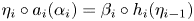
The folding of root lattices is classic [Reference Steinberg29] and plays a significant role in Lie theory when getting from the simply-laced cases to the non-simply-laced cases. The starting point is the fact that a symmetrizable generalized Cartan matrix $C$ is determined by a finite graph $\Gamma$
 with an admissible automorphism $\sigma$
 [Reference Lusztig23, Reference Steinberg29]. There is a surjective homomorphism, called the folding projection,
from the root lattice of $\Gamma$ to that of $C$
 , which preserves simple roots; see [Reference Springer28, Section 10.3]. Here, $\Gamma _0$
 denotes the set of vertices in $\Gamma$
 , and the orbit set $\Gamma _0/{\langle \sigma \rangle }$
 indexes both the rows and columns of $C$
 , so that we identify $\mathbb {Z}(\Gamma _0/{\langle \sigma \rangle })$
 with the root lattice of $C$
 . It is proved by [Reference Hubery17, Proposition 15] that the folding projection restricts to a surjective map
between the root systems [Reference Kac19], known as the folding of roots.
Let $\mathbb {K}$ be a field, and $\Delta$
 be a finite acyclic quiver such that its underlying graph is $\Gamma$
 . The path algebra $\mathbb {K}\Delta$
 is finite dimensional and hereditary. It is well known that the category of finite dimensional $\mathbb {K}\Delta$
 -modules, denoted by $\mathbb {K}\Delta {\rm -mod}$
 , categorifies the root lattice $\mathbb {Z}\Gamma _0$
 in the following manner [Reference Gabriel9]: the dimension vector ${\underline {\rm dim}}(M)$
 of any $\mathbb {K}\Delta$
 -module $M$
 belongs to $\mathbb {Z}\Gamma _0$
 , where simple $\mathbb {K}\Delta$
 -modules correspond to simple roots. Gabriel's theorem [Reference Gabriel9, 1.2 Satz], one of the foundations in modern representation theory of algebras, states that if $\Delta$
 is of Dynkin type, then indecomposable $\mathbb {K}\Delta$
 -modules correspond bijectively to positive roots in $\Phi (\Gamma )$
 .
.
Associated to a symmetrizable generalized Cartan matrix $C$ with a symmetrizer $D$
 and an acyclic orientation $\Omega$
 , a finite dimensional $1$
 -Gorenstein algebra $H$
 is defined in [Reference Geiss, Leclerc and Schröer11]. The category of finite dimensional $\tau$
 -locally free $H$
 -modules, denoted by $H {-{\rm mod}}^{\tau {-{\rm lf}}}$
 , categorifies the root lattice $\mathbb {Z}(\Gamma _0/{\langle \sigma \rangle })$
 in a similar manner: the rank vector $\underline {\rm rank}(X)$
 of any $\tau$
 -locally free $H$
 -module $X$
 belongs to $\mathbb {Z}(\Gamma _0/{\langle \sigma \rangle })$
 , where generalized simple $H$
 -modules correspond to simple roots. [Reference Geiss, Leclerc and Schröer11, Theorem 1.3], a remarkable analogue of Gabriel's theorem, states that if $C$
 is of Dynkin type, then indecomposable $\tau$
 -locally free $H$
 -modules correspond bijectively to positive roots in $\Phi (C)$
 .
.
We mention that the categorification in [Reference Geiss, Leclerc and Schröer11] works over an arbitrary ground field. In particular, it works for algebraically closed fields, and then certain geometric consideration for $\mathbb {K}\Delta$ carries over to $H$
 ; see [Reference Geiss10]. The traditional categorification of $\mathbb {Z}(\Gamma _0/{\langle \sigma \rangle })$
 for a non-symmetric Cartan matrix uses species [Reference Dlab and Ringel8], where the ground field has to be chosen suitably and can not be algebraically closed. We mention the work [Reference Hubery17], which studies the folding between root systems using skew group algebras associated to quivers with automorphisms.
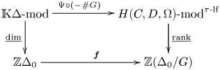
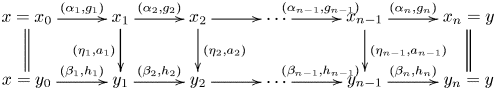
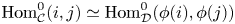
In view of the above work, the following question is natural and fundamental: how to categorify the folding projection $\boldsymbol {f}$ between the root lattices? More precisely, is there an additive functor $\Theta \colon \mathbb {K}\Delta {- \rm mod}\rightarrow H {- \rm mod}^{\tau \hbox{-}{\rm lf}}$
 making the following diagram

commute? Such a functor $\Theta$ might be called a categorification of $\boldsymbol {f}$
 , which will be viewed as a comparison between the work [Reference Gabriel9] and [Reference Geiss, Leclerc and Schröer11].
We will construct such a categorification under the assumptions that the characteristic ${\rm char}(\mathbb {K})=p$ of the field is positive and that the automorphism $\sigma$
 is of order $p^a$
 for some $a\geq 1$
 . Moreover, if $\Delta$
 is of Dynkin type, $\Theta$
 preserves indecomposable modules and categorifies the folding of positive roots. We emphasize that the assumption ${\rm char}(\mathbb {K})=p>0$
 is essential to ensure that $\Theta$
 preserves indecomposable modules; see remark 7.7 and theorem 7.8.
For our purpose, it is very natural to require that $\sigma$ preserves the orientation, that is, it acts on $\Delta$
 by quiver automorphisms. We will work in a slightly more general setting, namely, finite group actions on finite free EI categories.
Recall that a finite category is EI provided that each endomorphism is invertible; in particular, the endomorphism monoid of each object is a finite group. For example, the path category of a finite acyclic quiver is EI. The study of finite EI categories goes back to [Reference Lück24], and is used to reformulate and extend Alperin's weight conjecture [Reference Linckelmann22, Reference Webb33]. We mention that EI categories are very similar to graphs of groups in the sense of Bass–Serre [Reference Bass2, Reference Serre27].
As an EI analogue of a path category, the notion of a finite free EI category is introduced in [Reference Li21]. We are mostly interested in EI categories of Cartan type [Reference Chen and Wang4], which are certain finite free EI categories associated to symmetrizable generalized Cartan matrices. The construction of the categorification $\Theta$ relies on the isomorphism [Reference Chen and Wang4] between the category algebra of an EI category of Cartan type and the algebra $H$
 in [Reference Geiss, Leclerc and Schröer11].
1.2. The main results
Let $\mathcal {C}$ be a finite category and $G$
 be a finite group. Assume that $G$
 acts on $\mathcal {C}$
 by categorical automorphisms. As a very special case of the Grothendieck construction [Reference Grothendieck15], we have the skew group category $\mathcal {C}\rtimes G$
 . The terminology is justified by the following fact: the category algebra $\mathbb {K}(\mathcal {C}\rtimes G)$
 is isomorphic to $\mathbb {K}\mathcal {C}\#G$
 , the skew group algebra [Reference Reiten and Riedtmann26] of the category algebra $\mathbb {K}\mathcal {C}$
 with respect to the induced $G$
 -action. We mention that skew group algebras of Ginzburg dg algebras and their Jacobian algebras associated to quivers with potentials are studied in [Reference Giovannini and Pasquali14, Reference Le Meur20].
Following [Reference Li21, Definition 2.1], a finite EI quiver $(Q,\, U)$ consists of a finite acyclic quiver $Q$
 and an assignment $U$
 on $Q$
 . The assignment $U$
 assigns to each vertex $i$
 of $Q$
 a finite group $U(i)$
 , and to each arrow $\alpha$
 , a finite $(U(t\alpha ),\, U(s\alpha ))$
 -biset $U(\alpha )$
 . Here, $t\alpha$
 and $s\alpha$
 denote the terminating vertex and starting vertex of $\alpha$
 , respectively.
In a natural manner, each finite EI quiver $(Q,\, U)$ gives rise to a finite EI category $\mathcal {C}(Q,\, U)$
 such that the objects of $\mathcal {C}(Q,\, U)$
 are precisely the vertices of $Q$
 , the automorphism group of $i$
 coincides with $U(i)$
 , and that elements of $U(\alpha )$
 correspond to unfactorizable morphisms. By [Reference Li21, Definition 2.2 and Proposition 2.8], a finite EI category $\mathcal {C}$
 is said to be free, provided that it is equivalent to $\mathcal {C}(Q,\, U)$
 for some finite EI quiver $(Q,\, U)$
 .
.
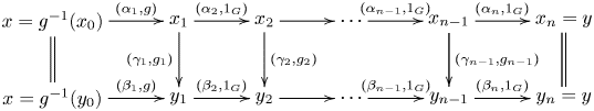
Let $G$ be a finite group acting on $(Q,\, U)$
 by EI quiver automorphisms. Then $G$
 acts naturally on the EI category $\mathcal {C}(Q,\, U)$
 . We form the skew group category $\mathcal {C}(Q,\, U)\rtimes G$
 . Inspired by [Reference Bass2, Section 3], we construct the ‘orbifold’ quotient EI quiver $(\overline {Q},\,\overline {U})$
 . Here, $\overline {Q}$
 is the quotient quiver $Q$
 by $G$
 , and the construction of the assignment $\overline {U}$
 is quite involved. We mention that for each vertex $\boldsymbol {i}$
 of $\overline {Q}$
 , the finite group $\overline {U}(\boldsymbol {i})$
 is a semi-direct product of $U(i)$
 with the stabilizer $G_i$
 for some vertex $i$
 of $Q$
 . For details, we refer to §§ 5.1.
The first main result identifies the category associated to the quotient EI quiver with the skew group category, and thus justifies the ‘orbifold’ quotient construction.
Theorem A Let $(Q,\, U)$ be a finite EI quiver with a $G$
 -action, and $(\overline {Q},\,\overline {U})$
 be its quotient EI quiver. Then there is an equivalence of categories
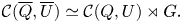
In general, it seems to be hard to describe the skeleton of a skew group category $\mathcal {C}\rtimes G$ explicitly. Theorem A (= theorem 5.3) actually shows that the skeleton of $\mathcal {C}(Q,\, U)\rtimes G$
 is isomorphic to $\mathcal {C}(\overline {Q},\,\overline {U})$
 .
.
We mention that theorem A might be viewed as a combinatorial analogue to the following well-known fact: the skew group algebra of a commutative algebra with respect to a finite group action is closely related to the corresponding quotient singularity; for example, see [Reference Wemyss34].
Let $\Delta$ be a finite acyclic quiver. Denote by $\mathcal {P}_\Delta$
 its path category. We view $\Delta$
 as a finite EI quiver $(\Delta,\,U_{\rm tr})$
 with trivial assignment $U_{\rm tr}$
 . Then we have
Assume that $G$ acts on $\Delta$
 by quiver automorphisms. It induces a $G$
 -action on $(\Delta,\,U_{\rm tr})$
 . Denote by $(\overline {\Delta },\,\overline {U}_{\rm tr})$
 the corresponding quotient EI quiver, where $\overline {\Delta }$
 is the quotient quiver $\Delta$
 by $G$
 . Theorem A implies that there is an equivalence of categories
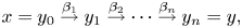
By a Cartan triple $(C,\,D,\,\Omega )$ , we mean that $C$
 is a symmetrizable generalized Cartan matrix, $D$
 is its symmetrizer and that $\Omega$
 is an acyclic orientation of $C$
 . Following [Reference Geiss, Leclerc and Schröer11, Section 1.4], we denote by $H(C,\, D,\, \Omega )$
 the $1$
 -Gorenstein $\mathbb {K}$
 -algebra associated to any Cartan triple $(C,\, D,\, \Omega )$
 . Similarly, we associate a finite free EI category $\mathcal {C}(C,\,D,\,\Omega )$
 , called an EI category of Cartan type, to any Cartan triple $(C,\, D,\, \Omega )$
 ; see [Reference Chen and Wang4, Definition 4.1].
It is well known that there is a Cartan triple $(C,\,D,\,\Omega )$ associated to the above $G$
 -action on $\Delta$
 such that both the rows and columns of $C$
 and $D$
 are indexed by the orbit set $\overline {\Delta }_0=\Delta _0/G$
 . Here, $\Delta _0$
 denotes the set of vertices in $\Delta$
 . Moreover, for each $G$
 -orbit $\boldsymbol {i}$
 of vertices, the corresponding diagonal entry of $D$
 is $|G|/|\boldsymbol {i}|$
 ; the corresponding off-diagonal entry of $C$
 is
is
where $|\boldsymbol {i}|$ denotes the cardinality of the $G$
 -orbit $\boldsymbol {i}$
 and $N_{\boldsymbol {i},\,\boldsymbol {j}}$
 denotes the number of arrows in $\Delta$
 between the $G$
 -orbit $\boldsymbol {i}$
 and $G$
 -orbit $\boldsymbol {j}$
 . The orientation of $\Omega$
 is induced from the one of $\Delta$
 .
.
The second main theorem establishes an equivalence between the skew group category and the EI category of Cartan type. Based on [Reference Chen and Wang4], we obtain a Morita equivalence between the skew group algebra $\mathbb {K}\Delta \#G$ and $H(C,\, D,\, \Omega )$
 .
.
Theorem B Let $\Delta$ be a finite acyclic quiver with a $G$
 -action that satisfies $({\dagger} 1)\mbox {-}({\dagger} 3)$
 in §§ 6.2. Assume that $(C,\,D,\,\Omega )$
 is the associated Cartan triple. Then we have the following statements.
(1) There is an equivalence of categories
\[ \mathcal{P}_{\Delta}\rtimes G\simeq \mathcal{C}(C,D,\Omega). \]
(2) Assume that ${\rm char}(\mathbb {K})=p>0$
and that $G$ is a $p$-group. Then the skew group algebras $\mathbb {K}\Delta \#G$ and $H(C,\,D,\,\Omega )$ are Morita equivalent.


The above technical conditions $({\dagger} 1)\mbox {-}({\dagger} 3)$ are easily satisfied when $G$
 is cyclic. On the other hand, examples where they do hold seem to be ubiquitous; see example 6.7. In view of (1.1), the core of the proof of theorem B is to describe the assignment $\overline {U}_{\rm tr}$
 in the quotient EI quiver. We refer to theorem 6.6 for more details.
The equivalence and the Morita equivalence in theorem B indicate that both EI categories of Cartan type [Reference Chen and Wang4] and the algebra $H(C,\,D,\, \Omega )$ [Reference Geiss, Leclerc and Schröer11] arise naturally in the representation theory of quivers with automorphisms [Reference Hubery17, Reference Lusztig23].
In what follows, we describe an application of theorem B, namely a categorification of the folding projection. Consequently, in the Dynkin cases, we give a new interpretation of the indecomposable modules in [Reference Geiss, Leclerc and Schröer11] that categorify the root system $\Phi ^+(C)$ : they are essentially the induced modules of indecomposable modules over the path algebra.
The Morita equivalence in theorem B(2) yields an equivalence between module categories

We have the obvious induction functor

For $\tau$ -locally free modules over $H=H(C,\, D,\, \Omega )$
 , we refer to [Reference Geiss, Leclerc and Schröer11, Definition 1.1 and Section 11]. Denote by $H\mbox {-mod}^{\tau \mbox {-lf}}$
 the full subcategory of $H\mbox {-mod}$
 consisting of $\tau$
 -locally free modules. In contrast to [Reference Geiss, Leclerc and Schröer11], we do not require $\tau$
 -locally free $H$
 -modules to be indecomposable.
Recall that $\mathbb {Z}\Delta _0$ and $\mathbb {Z}(\Delta _0/G)$
 denote the root lattices of $\Delta$
 and $C$
 , respectively. The sets of positive roots are denoted by $\Phi ^+(\Delta )$
 and $\Phi ^+(C)$
 , respectively.
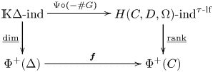
The third main result shows that the composite functor $\Psi \circ (-\#G)$ is the pursued categorification of the folding projection $\boldsymbol {f}$
 ; see theorem 7.8 and proposition 7.9.
Theorem C Assume that ${\rm char}(\mathbb {K})=p>0$ and that $G$
 is a cyclic $p$
 -group. Assume that $G$
 acts on a finite acyclic quiver $\Delta$
 such that $G_{\alpha }=G_{s(\alpha )}\cap G_{t(\alpha )}$
 for each arrow $\alpha$
 in $\Delta$
 . Assume that $(C,\,D,\,\Omega )$
 is its associated Cartan triple. Then we have the following commutative diagram.
Assume further that $\Delta$ is of Dynkin type. Then the above commutative diagram restricts to the following one.
Here, $G_\alpha$ , $G_{s(\alpha )}$
 and $G_{t(\alpha )}$
 denote the stabilizers of an arrow $\alpha$
 , its starting vertex $s(\alpha )$
 and terminating vertex $t(\alpha )$
 , respectively. The natural condition $G_{\alpha }=G_{s(\alpha )}\cap G_{t(\alpha )}$
 implies that the technical conditions $({\dagger} 1)\mbox {-}({\dagger} 3)$
 in theorem B hold.
In (1.2), we denote by $\mathbb {K}\Delta \mbox {-ind}$ a complete set of representatives of indecomposable $\mathbb {K}\Delta$
 -modules. Similarly, $H(C,\,D,\,\Omega )\text {- ind}^{\tau \text {- lf}}$
 is a complete set of representatives of indecomposable $\tau$
 -locally free $H(C,\, D,\, \Omega )$
 -modules.
In the Dynkin cases, by [Reference Gabriel9, 1.2 Satz] and [Reference Geiss, Leclerc and Schröer11, Theorem 1.3], the vertical arrows in (1.2) are both bijections. Since $\boldsymbol {f}\colon \Phi ^+(\Delta )\rightarrow \Phi ^+(C)$ is surjective, we infer that up to the equivalence $\Psi$
 , every $\tau$
 -locally free $H(C,\, D,\, \Omega )$
 -module is induced from $\mathbb {K}\Delta \mbox {-ind}$
 . This yields a new interpretation of those $H(C,\, D,\, \Omega )$
 -modules [Reference Geiss, Leclerc and Schröer11] that categorify the root system $\Phi ^+(C)$
 .
.
In view of [Reference Lusztig23, Section 14.1] and [Reference Hubery17], it has been expected that skew group algebras play a role in categorifying the root lattice for symmetrizable generalized Cartan matrices. We observe that in [Reference Hubery17, Section 4] the characteristic of the ground field is assumed to be coprime to the order of the acting group. In contrast, the feature of theorem C is the assumptions that the ground field $\mathbb {K}$ is of characteristic $p$
 and that the order of the acting group $G$
 is a $p$
 -power.
1.3. The structure
The paper is structured as follows. In § 2, we prove that for a finite group action on a finite category, the skew group category is EI if and only if so is the given category; see proposition 2.5. In § 3, we study the unique factorization property of morphisms and free EI categories. We prove that for an action of a finite group on a finite category, the skew group category is free EI if and only if so is the given category; see corollary 3.4. In § 4, we recall finite EI quivers introduced in [Reference Li21], and prove a universal property of the free EI category associated to a finite EI quiver; see proposition 4.2.
For an action of a finite group on a finite EI quiver, we construct its ‘orbifold’ quotient EI quiver explicitly in § 5. Theorem 5.3 states that the category associated to the quotient EI quiver is equivalent to the skew group category.
In § 6, we recall the algebras $H$ [Reference Geiss, Leclerc and Schröer11] and EI categories [Reference Chen and Wang4] associated to Cartan triples. For an action of a finite group on a finite acyclic quiver, we give sufficient conditions such that the quotient EI quiver is of Cartan type. Consequently, the skew group algebra of the path algebra is Morita equivalent to the algebra $H$
 ; see theorem 6.6.
In the final section, we first study induced modules over skew group algebras. We apply theorem 6.6 to the case that a finite cyclic $p$ -group acts on a finite acyclic quiver. Theorem 7.8 obtains a categorification of the folding projection $\boldsymbol {f}$
 , namely an additive functor from the module category over the path algebra to the category of $\tau$
 -locally free $H$
 -modules. In the Dynkin cases, restricting the categorification to indecomposable modules, we obtain a categorification of the folding of positive roots; see proposition 7.9. In the end, we give an explicit example to illustrate the categorification.
By default, a module means a finite dimensional left module. For a finite dimensional algebra $A$ , we denote by $A\mbox {-mod}$
 the abelian category of finite dimensional left $A$
 -modules. We use ${\rm rad}(A)$
 to denote the Jacobson radical of $A$
 . The unadorned tensor $\otimes$
 means the tensor product over the ground field $\mathbb {K}$
 .
.
2. Skew group categories
In this section, we fix the notation by recalling basic facts about finite group actions on finite categories. The EI property of a skew group category is studied in proposition 2.5.
2.1. Finite $G$-categories

Let $\mathcal {C}$ be a finite category, that is, a category with only finitely many morphisms. As any object is determined by its identity endomorphism, the finite category $\mathcal {C}$
 necessarily has only finitely many objects. Denote by ${\rm Obj}(\mathcal {C})$
 (resp. ${\rm Mor}(\mathcal {C})$
 ) the finite set of objects (resp. morphisms) in $\mathcal {C}$
 .
.
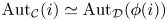
Recall that an automorphism on $\mathcal {C}$ is a fully faithful endofunctor which is bijective on objects. Therefore, such an automorphism has a genuine inverse. We denote by ${\rm Aut}(\mathcal {C})$
 the automorphism group of $\mathcal {C}$
 , whose elements are automorphisms on $\mathcal {C}$
 and whose multiplication is given by the composition of automorphisms.
Let $G$ be a finite group with its unit $1_G$
 . A finite $G$
 -category $\mathcal {C}$
 is a finite category equipped with a group homomorphism
To simplify the notation, the following convention will be used: for $g\in G$ and $x\in {\rm Obj}(\mathcal {C})$
 , we write $g(x)=\rho (g)(x)$
 ; for $\alpha \in {\rm Mor}(\mathcal {C})$
 , we write $g(\alpha )=\rho (g)(\alpha )$
 .
.
For a finite $G$ -category $\mathcal {C}$
 , we will recall the skew group category $\mathcal {C}\rtimes G$
 ; compare [Reference Reiten and Riedtmann26, Subsection 3.1] and [Reference Cibils and Marcos5, Definition 2.3]. It has the same objects as $\mathcal {C}$
 ; for two objects $x$
 and $y$
 , the corresponding Hom set is defined to be

For any morphisms $(\alpha,\,g)\in {\rm Hom}_{\mathcal {C}\rtimes G}(x,\,y)$ and $(\beta,\,h)\in {\rm Hom}_{\mathcal {C}\rtimes G}(y,\,z)$
 , the composition is defined by

We observe that the identity endomorphism of $x$ in $\mathcal {C}\rtimes G$
 is given by $({\rm Id}_x,\, 1_G)$
 , where ${\rm Id}_x$
 is the identity endomorphism of $x$
 in $\mathcal {C}$
 . We mention that the formation of a skew group category might be viewed as a very special case of the Grothendieck construction; compare [Reference Grothendieck15, VI.8], [Reference Webb32, Section 7] and [Reference Xu35, Subsection 2.1].
Let $\mathbb {K}$ be a field and $\mathcal {C}$
 be a finite category. The category algebra $\mathbb {K}\mathcal {C}$
 of $\mathcal {C}$
 is a finite dimensional $\mathbb {K}$
 -algebra defined as follows. As a $\mathbb {K}$
 -vector space, $\mathbb {K}\mathcal {C}=\bigoplus \limits _{\alpha \in {\rm Mor}(\mathcal {C})} \mathbb {K}\alpha$
 , and the product between the basis elements is given by the following rule:
The unit of $\mathbb {K}\mathcal {C}$ is given by $1_{\mathbb {K}\mathcal {C}}=\sum \limits _{x \in {\rm Obj}(\mathcal {C})}{\rm Id}_x$
 .
.
Denote by $(\mathbb {K}\mbox {-mod})^\mathcal {C}$ the category of covariant functors from $\mathcal {C}$
 to $\mathbb {K}\mbox {-mod}$
 . There is a canonical equivalence

sending a $\mathbb {K}\mathcal {C}$ -module $M$
 to the functor ${\rm can}(M)\colon \mathcal {C}\rightarrow \mathbb {K}\mbox {-mod}$
 described as follows: ${\rm can}(M)(x)={\rm Id}_x.M$
 for each object $x$
 in $\mathcal {C}$
 ; for any morphism $\alpha \colon x\rightarrow y$
 , we have

For details, we refer to [Reference Webb32, Proposition 2.1].
Denote by ${\rm Aut}(\mathbb {K}\mathcal {C})$ the group of algebra automorphisms on $\mathbb {K}\mathcal {C}$
 . Each categorical automorphism on $\mathcal {C}$
 induces uniquely an algebra automorphism on $\mathbb {K}\mathcal {C}$
 . Therefore, there is a canonical embedding of groups
Assume that $\mathcal {C}$ is a finite $G$
 -category. The group homomorphism $\rho \colon G\rightarrow {\rm Aut}(\mathcal {C})$
 induces a group homomorphism $\rho '\colon G\rightarrow {\rm Aut}(\mathbb {K}\mathcal {C})$
 . In other words, the group $G$
 acts on the algebra $\mathbb {K}\mathcal {C}$
 by algebra automorphisms. We denote by $\mathbb {K}\mathcal {C}\# G$
 the corresponding skew group algebra. Here, we recall that $\mathbb {K}\mathcal {C}\# G=\mathbb {K}\mathcal {C}\otimes \mathbb {K}G$
 as a $\mathbb {K}$
 -vector space, where the tensor product $\alpha \otimes g$
 is written as $\alpha \#g$
 . The multiplication is given by

for any $\alpha,\, \beta \in {\rm Mor}(\mathcal {C})$ and $g,\, h\in G$
 . We emphasize that on the right hand side, $\beta h(\alpha )$
 means the product of $\beta$
 and $h(\alpha )$
 in $\mathbb {K}\mathcal {C}$
 , namely, the composition $\beta \circ h(\alpha )$
 in $\mathcal {C}$
 .
.
The following easy observation, extending [Reference Xu36, Lemma 2.3.2], justifies the terminology ‘skew group category’.
Proposition 2.1 Let $\mathcal {C}$ be a finite $G$
 -category. Then there is an isomorphism of algebras
sending a morphism $(\alpha,\, g)$ in $\mathcal {C}\rtimes G$
 to the element $\alpha \# g$
 in $\mathbb {K}\mathcal {C}\#G$
 .
.
In the following lemma, we collect elementary facts on skew group categories.
Lemma 2.2 Let $\mathcal {C}$ be a finite $G$
 -category. Then the following two statements hold.
(1) A morphism $(\alpha,\,g)$
in $\mathcal {C}\rtimes G$ is an isomorphism if and only if $\alpha$ is an isomorphism in $\mathcal {C}$.(2) For two objects $x$
and $y$ in $\mathcal {C}$, they are isomorphic in $\mathcal {C}\rtimes G$ if and only if $x$ is isomorphic to $g(y)$ in $\mathcal {C}$ for some $g\in G$.


Proof. (1) For the ‘if’ part, we assume that $\alpha ^{-1}$ is the inverse of $\alpha$
 in $\mathcal {C}$
 . Then $(g^{-1}(\alpha ^{-1}),\, g^{-1})$
 is a well-defined morphism in $\mathcal {C}\rtimes G$
 ; moreover, it is the required inverse of $(\alpha,\, g)$
 .
.
For the ‘only if’ part, we observe that the inverse of $(\alpha,\, g)$ has to be of the form $(\beta,\, g^{-1})$
 . Then it is direct to see that $g(\beta )$
 is the inverse of $\alpha$
 , as required.
(2) For the ‘if’ part, we assume that $\alpha \colon g(y) \rightarrow x$
is an isomorphism in $\mathcal {C}$. Then $(\alpha,\, g)$ is a morphism from $y$ to $x$ in $\mathcal {C}\rtimes G$; moreover, by (1) it is an isomorphism between $y$ and $x$.


For the ‘only if’ part, we assume that $(\alpha,\, g)\in {\rm Hom}_{\mathcal {C}\rtimes G}(y,\, x)$ is an isomorphism. By (1), we deduce that $\alpha$
 is an isomorphism from $g(y)$
 to $x$
 in $\mathcal {C}$
 .
.
2.2. The EI property
Let $\mathcal {C}$ be a finite $G$
 -category as above. For each object $x$
 in $\mathcal {C}$
 , we denote by $G_x=\{g\in G \mid g(x)=x\}$
 its stabilizer. We observe that $G_x$
 acts on the monoid ${\rm Hom}_\mathcal {C}(x,\, x)$
 by monoid automorphisms. Denote by ${\rm Hom}_\mathcal {C}(x,\, x)\rtimes G_x$
 the corresponding semi-direct product. There is an inclusion between monoids

The following terminology is inspired by [Reference Lusztig23, Subsection 12.1.1].
Definition 2.3 A finite $G$ -category $\mathcal {C}$
 is admissible, provided that for any $x\in {\rm Obj}(\mathcal {C})$
 and $g\in G$
 , ${\rm Hom}_{\mathcal {C}}(g(x),\,x)=\emptyset$
 whenever $g(x)\neq x$
 .
.
Lemma 2.4 A finite $G$ -category $\mathcal {C}$
 is admissible if and only if ${\rm inc}_x$
 is surjective for each object $x$
 in $\mathcal {C}$
 .
.
Proof. The inclusion ${\rm inc}_x$ is not surjective if and only if there exists $g\in G$
 satisfying $g(x)\neq x$
 and ${\rm Hom}_\mathcal {C}(g(x),\, x)\neq \emptyset$
 . Then the result follows immediately.
Recall from [Reference Webb32] that a finite category $\mathcal {C}$ is EI if every endomorphism is an isomorphism. Therefore, for each object $x$
 , ${\rm Hom}_{\mathcal {C}}(x,\,x)={\rm Aut}_{\mathcal {C}}(x)$
 is a finite group. Finite EI categories are of interest from many different perspectives; for example, see [Reference Webb33, Reference Xu36].
Proposition 2.5 Let $\mathcal {C}$ be a finite $G$
 -category. Then $\mathcal {C}$
 is an EI category if and only if so is $\mathcal {C}\rtimes G$
 .
.
Proof. For the ‘if’ part, we assume that $\mathcal {C}\rtimes G$ is an EI category. For any $\alpha \in {\rm Hom}_{\mathcal {C}}(x,\,x)$
 , $(\alpha,\,1_G)$
 is an endomorphism of $x$
 in $\mathcal {C}\rtimes G$
 . Since $\mathcal {C}\rtimes G$
 is EI, $(\alpha,\, 1_G)$
 is an isomorphism. By lemma 2.2(1), the endomorphism $\alpha$
 is an isomorphism in $\mathcal {C}$
 , as required.
For the ‘only if’ part, we assume that $\mathcal {C}$ is an EI category. Any endomorphism of $x$
 in $\mathcal {C}\rtimes G$
 is of the form $(\alpha,\, g)$
 , where $\alpha \colon g(x)\rightarrow x$
 is a morphism in $\mathcal {C}$
 . Assume that $g^d=1_G$
 for some $d\geq 1$
 . Then we have a chain

of morphisms in $\mathcal {C}$ . Since $\mathcal {C}$
 is EI, it follows that all the morphisms in the chain are isomorphisms. In particular, the morphism $\alpha$
 is an isomorphism. Applying lemma 2.2(1), we infer that the endomorphism $(\alpha,\, g)$
 is an isomorphism, proving that $\mathcal {C}\rtimes G$
 is an EI category.
The following corollary follows immediately from lemma 2.4.
Corollary 2.6 Let $\mathcal {C}$ be a finite admissible $G$
 -category. Assume that $\mathcal {C}$
 is EI. Then for each object $x$
 , we have an identification of groups

3. Free EI categories
In this section, we study the unique factorization property of morphisms and free EI categories [Reference Li21]. We prove that the unique factorization property of a morphism in a skew group category is completely determined by the one of the underlying morphism in the given category; see proposition 3.3. Then we conclude that a skew group category is free EI if and only if so is the given category; see corollary 3.4.
Let $\mathcal {C}$ be a finite category. Recall from [Reference Li21, Definition 2.3] that a morphism $\alpha \colon x\rightarrow y$
 in $\mathcal {C}$
 is unfactorizable, if it is a non-isomorphism and whenever it has a factorization $x \overset {\beta }{\rightarrow } z \overset {\gamma }{\rightarrow } y$
 , then either $\beta$
 or $\gamma$
 is an isomorphism. We observe that if $\alpha \colon x \rightarrow y$
 is unfactorizable, then so is $h\circ \alpha \circ g$
 for any isomorphism $h$
 and $g$
 .
.
As the notion of an unfactorizable morphism is categorical, it is preserved by any categorical automorphism. Then the following observation is clear.
Lemma 3.1 Let $G$ be a finite group and $\mathcal {C}$
 be a finite $G$
 -category. Then for any morphism $\alpha$
 in $\mathcal {C}$
 and $g\in G$
 , $\alpha$
 is unfactorizable if and only if so is $g(\alpha )$
 .
.
We say that a morphism $\alpha$ in a finite category $\mathcal {C}$
 satisfies the Unique Factorization Property (UFP), if it is either an isomorphism or, whenever it has two factorizations into unfactorizable morphisms:

and
then $m=n$ , and there are isomorphisms $\gamma _i\colon x_i \rightarrow y_i$
 in $\mathcal {C}$
 for $1\leq i\leq m-1$
 , such that the following diagram commutes.
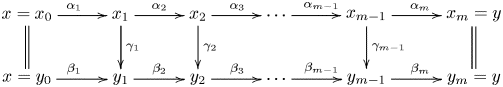
We mention that, in general, a non-isomorphism in a finite category $\mathcal {C}$ might not have a factorization into unfactorizable morphisms. However, if $\mathcal {C}$
 is EI, any non-isomorphism in $\mathcal {C}$
 has a factorization into unfactorizable morphisms; see [Reference Li21, Proposition 2.6].
Lemma 3.2 Let $G$ be a finite group and $\mathcal {C}$
 be a finite $G$
 -category. Then a morphism $(\alpha,\,g)$
 in $\mathcal {C}\rtimes G$
 is unfactorizable if and only if $\alpha$
 is unfactorizable in $\mathcal {C}$
 .
.
Proof. By lemma 2.2(1), we observe that $(\alpha,\,g)$ is a non-isomorphism if and only if so is $\alpha$
 .
.
For the ‘if’ part, we assume that $\alpha$ is unfactorizable. Suppose we have a factorization

in $\mathcal {C}\rtimes G$ . The factorization $\alpha =\beta \circ h(\gamma )$
 in $\mathcal {C}$
 implies that either $\beta$
 or $h(\gamma )$
 is an isomorphism. As $h\in G$
 induces a categorical automorphism on $\mathcal {C}$
 , we infer that $h(\gamma )$
 is an isomorphism if and only if so is $\gamma$
 . In view of lemma 2.2(1), we infer that either $(\beta,\, h)$
 or $(\gamma,\, k)$
 is an isomorphism in $\mathcal {C}\rtimes G$
 , proving that $(\alpha,\, g)$
 is unfactorizable.
For the ‘only if’ part, we assume that $(\alpha,\,g)$ is unfactorizable. Assume on the contrary that $\alpha =\beta \circ \gamma$
 with both $\beta$
 and $\gamma$
 non-isomorphisms in $\mathcal {C}$
 . Then we have

By lemma 2.2(1), we have that both $(\beta,\,1_G)$ and $(\gamma,\,g)$
 are non-isomorphisms in $\mathcal {C}\rtimes G$
 . This contradicts to the unfactorizability of $(\alpha,\, g)$
 .
.
The following main result of this section characterizes the UFP of morphisms in a skew group category.
Proposition 3.3 Let $G$ be a finite group and $\mathcal {C}$
 be a finite $G$
 -category. Then a morphism $(\alpha,\,g)$
 in $\mathcal {C}\rtimes G$
 satisfies the UFP if and only if $\alpha$
 satisfies the UFP in $\mathcal {C}$
 .
.
Proof. By lemma 2.2(1), the morphism $(\alpha,\, g)$ is an isomorphism if and only if so is $\alpha$
 . In the following proof, we will assume that both $(\alpha,\, g)$
 and $\alpha \colon g(x)\rightarrow y$
 are non-isomorphisms.
For the ‘if’ part, we assume that $\alpha \colon g(x)\rightarrow y$ satisfies the UFP in $\mathcal {C}$
 . Suppose that $(\alpha,\,g)\colon x\rightarrow y$
 has two factroizations into unfactorizable morphisms in $\mathcal {C}\rtimes G$
 :
:

and

The factorizations imply $g_n\cdots g_1=g=h_m\cdots h_1$ in $G$
 . Moreover, the morphism $\alpha \colon g(x)\rightarrow y$
 has two factorizations in $\mathcal {C}$
 :
:

and

Here, in the first factorization we use $g(x)=g_n\cdots g_2g_1(x_0)$ , and in the second one we use $g(x)=h_m\cdots h_2h_1(x_0)$
 . By lemmas 3.1 and 3.2, all the morphisms appearing in the above two factorizations are unfactorizable in $\mathcal {C}$
 .
.
Since $\alpha$ satisfies the UFP, we infer that $n=m$
 , and that there are isomorphisms $\theta _i: g_n\cdots g_{i+1}(x_i)\rightarrow h_n\cdots h_{i+1}(y_{i})$
 , $1\leq i\leq n-1$
 , such that the following diagram in $\mathcal {C}$
 commutes.
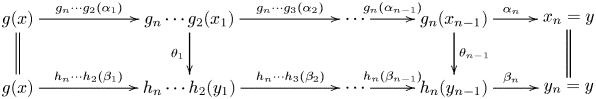
Set $\theta _0={\rm Id}_{g(x)}$ and $\theta _n={\rm Id}_y$
 . Then the above commutativity implies that

for each $1\leq i\leq n$ . The identity for the case $i=n$
 means $\alpha _n=\beta _n\circ \theta _{n-1}$
 .
.
For each $1\leq i\leq n-1$ , we set $a_{i}=h_{i+1}^{-1}\cdots h_n^{-1}g_n\cdots g_{i+1}$
 . In addition, we set $a_0=1_G=a_n$
 . Then we have
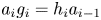
for each $1\leq i\leq n$ . Here, to see $a_1g_1=h_1$
 , we use the fact that $g_n\cdots g_1=h_n\cdots h_1$
 .
.
For each $1\leq i\leq n$ , we set $\eta _{i}=h_{i+1}^{-1}\cdots h_n^{-1}(\theta _{i})$
 . We observe $\eta _0={\rm Id}_x$
 and $\eta _n={\rm Id}_y$
 . Then each $\eta _i\colon a_i(x_i)\rightarrow y_i$
 is an isomorphism in $\mathcal {C}$
 . Consequently, by lemma 2.2(1) we have an isomorphism $(\eta _i,\, a_i)\colon x_i\rightarrow y_i$
 in $\mathcal {C}\rtimes G$
 .
.
Applying $h_{i+1}^{-1}\cdots h_n^{-1}$ to (3.1), we have
for each $1\leq i\leq n$ . By (3.2) and (3.3), we have the following commutative diagram in $\mathcal {C}\rtimes G$
 .
.
This implies that the morphism $(\alpha,\,g)$ satisfies the UFP.
The proof of the ‘only if’ is similar and actually easier. We assume that $(\alpha,\,g)\colon x\rightarrow y$ satisfies the UFP in $\mathcal {C}\rtimes G$
 . Suppose that $\alpha \colon g(x)\rightarrow y$
 has two factorizations into unfactorizable morphisms in $\mathcal {C}$
 :
:

and

Then the morphism $(\alpha,\,g)\colon x\rightarrow y$ in $\mathcal {C}\rtimes G$
 has two factorizations:

and

By lemma 3.2, all the morphisms $(\alpha _1,\,g)$ , $(\beta _1,\,g)$
 , $(\alpha _i,\,1_G)$
 and $(\beta _j,\, 1_G)$
 are unfactorizable, for $2\leq i\leq n$
 and $2\leq j\leq m$
 .
.
Since the morphism $(\alpha,\,g)$ satisfies the UFP, then $m=n$
 and there are isomorphisms $(\gamma _i,\, g_i)\colon x_i\rightarrow y_i$
 , $1\leq i\leq n-1$
 , such that the following diagram in $\mathcal {C}\rtimes G$
 commutes.
The commutativity implies $g_1=g_2=\cdots =g_{n-1}=1_G$ . By lemma 2.2(1), each $\gamma _i\colon x_i\rightarrow y_i$
 is an isomorphism in $\mathcal {C}$
 . Consequently, the isomorphisms $\gamma _i$
 make the following diagram in $\mathcal {C}$
 commute.

This proves that $\alpha$ satisfies the UFP, as required.
Recall that a finite EI category $\mathcal {C}$ is free provided that each morphism satisfies the UFP; compare [Reference Li21, Definition 2.7 and Proposition 2.8]. For an alternative characterization of a free EI category, we refer to [Reference Wang31, Proposition 4.5].
The following result follows immediately from propositions 2.5 and 3.3.
Corollary 3.4 Let $\mathcal {C}$ be a finite $G$
 -category. Then $\mathcal {C}$
 is a free EI category if and only if so is $\mathcal {C}\rtimes G$
 .
.
Remark 3.5 The above argument of corollary 3.4 uses the combinatorial result, namely proposition 3.3. Let us sketch another proof of corollary 3.4 using category algebras. By proposition 2.5, we may assume that both $\mathcal {C}$ and $\mathcal {C}\rtimes G$
 are EI categories.
Take an arbitrary field $\mathbb {K}$ of characteristic zero. By proposition 2.1, we identify the category algebra $\mathbb {K}(\mathcal {C}\rtimes G)$
 with the skew group algebra $\mathbb {K}\mathcal {C}\# G$
 . It is well known that $\mathbb {K}\mathcal {C}$
 is hereditary if and only if so is $\mathbb {K}\mathcal {C}\#G$
 ; see [Reference Reiten and Riedtmann26, Theorems 1.3(c) and 1.4]. Then corollary 3.4 follows immediately from the following result due to [Reference Li21, Theorem 5.3]: the EI category $\mathcal {C}$
 (resp. $\mathcal {C}\rtimes G$
 ) is free if and only if the corresponding category algebra $\mathbb {K}\mathcal {C}$
 (resp. $\mathbb {K}(\mathcal {C}\rtimes G)$
 ) is hereditary.
4. Finite EI quivers and $G$-actions

In this section, we recall basic facts on finite EI quivers. We prove a universal property of the free EI category associated to a finite EI quiver; see proposition 4.2. We study finite group actions on finite EI quivers.
4.1. Categories associated to finite EI quivers
Let $Q=(Q_0,\, Q_1; s,\,t)$ be a finite quiver, where $Q_0$
 and $Q_1$
 are the finite sets of vertices and arrows, respectively. The maps $s,\, t\colon Q_1\rightarrow Q_0$
 assign to each arrow $\alpha$
 its starting vertex $s(\alpha )$
 and terminating vertex $t(\alpha )$
 , respectively.
A path $p=\alpha _n\cdots \alpha _2\alpha _1$ of length $n$
 in $Q$
 consists of arrows $\alpha _i$
 satisfying $t(\alpha _i)=s(\alpha _{i+1})$
 for each $1\leq i\leq n-1$
 . Here, we write concatenation from right to left. We set $s(p)=s(\alpha _1)$
 and $t(p)=t(\alpha _n)$
 . An arrow is identified with a path of length one. To each vertex $i\in Q_0$
 , we associate a trivial path $e_i$
 of length zero, satisfying $s(e_i)=i=t(e_i)$
 .
.
A finite quiver $Q$ is said to be acyclic, provided that there is no oriented cycle in $Q$
 , that is, there is no nontrivial path with the same starting and terminating vertex. This is equivalent to the condition that there are only finitely many paths in $Q$
 .
.
Let $H$ be a finite group, and let $X$
 be a right $H$
 -set, that is, $H$
 acts on $X$
 on the right. Let $Y$
 be a left $H$
 -set. The biset product $X\times _H Y$
 is defined to be the set

of equivalence classes with respect to the equivalence relation $\sim$ given by $(x.h,\, y)\sim (x,\, h.y)$
 for $x\in X,\, h\in H$
 and $y\in Y$
 . By abuse of notation, the elements in $X\times Y/\sim$
 are still denoted by $(x,\,y)$
 for $x\in X$
 and $y\in Y$
 .
.
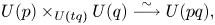
Let $G$ and $K$
 be finite groups. By a $(G,\, H)$
 -biset $X$
 , we mean a set $X$
 which is a left $G$
 -set and a right $H$
 -set satisfying $(g.x).h=g.(x.h)$
 for any $g\in G$
 , $x\in X$
 and $h\in H$
 . Here, we use the dot to denote the group actions. Let $Y$
 be a $(H,\, K)$
 -biset. Then the biset product $X\times _H Y$
 is naturally a $(G,\, K)$
 -biset.
Example 4.1 Let $\mathcal {C}$ be a finite EI category. For any two objects $x$
 and $y$
 , the ${\rm Hom}$
 -set ${\rm Hom}_\mathcal {C}(x,\, y)$
 is naturally an $({\rm Aut}_\mathcal {C}(y),\, {\rm Aut}_\mathcal {C}(x))$
 -biset, where the actions are given by the composition of morphisms in $\mathcal {C}$
 .
.
Denote by ${\rm Hom}^0_\mathcal {C}(x,\, y)$ the subset of ${\rm Hom}_\mathcal {C}(x,\, y)$
 consisting of unfactorizable morphisms. As unfactorizable morphisms are closed under composition with isomorphisms, ${\rm Hom}^0_\mathcal {C}(x,\, y)$
 is an $({\rm Aut}_\mathcal {C}(y),\, {\rm Aut}_\mathcal {C}(x))$
 -sub-biset of ${\rm Hom}_\mathcal {C}(x,\, y)$
 .
.
Recall from [Reference Li21, Definition 2.1] that a finite EI quiver $(Q,\, U)$ consists of a finite acyclic quiver $Q$
 and an assignment $U=(U(i),\, U(\alpha ))_{i\in Q_0, \alpha \in Q_1}$
 . In more details, for each vertex $i\in Q_0$
 , $U(i)$
 is a finite group, and for each arrow $\alpha \in Q_1$
 , $U(\alpha )$
 is a finite $(U(t\alpha ),\, U(s\alpha ))$
 -biset. Here, we emphasize that each $U(\alpha )$
 is nonempty.
For any path $p=\alpha _n\cdots \alpha _2\alpha _1$ in $Q$
 , we define

Then $U(p)$ is naturally a $(U(tp),\, U(sp))$
 -biset. A typical element in $U(p)$
 will be denoted by $(u_n,\, \cdots,\, u_2,\, u_1)$
 with each $u_i\in U(\alpha _i)$
 . For each vertex $i\in Q_0$
 , we identify $U(e_i)$
 with $U(i)$
 .
.
For two paths $p,\, q$ satisfying $s(p)=t(q)$
 , we have a natural isomorphism of $(U(tp),\, U(sq))$
 -bisets
sending $((u_m',\,\cdots,\, u_1'),\, (u_n,\, \cdots,\, u_1))$ to $(u_m',\, \cdots,\, u_1',\, u_n,\, \cdots,\, u_1)$
 , where $pq$
 denotes the concatenation of paths.
Each finite EI quiver $(Q,\, U)$ gives rise to a finite EI category $\mathcal {C}(Q,\, U)$
 ; see [Reference Li21, Section 2]. The objects of $\mathcal {C}(Q,\, U)$
 coincide with the vertices of $Q$
 . For two objects $i$
 and $j$
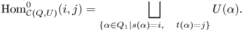
 , we have a disjoint union

The composition of morphisms is induced by the concatenation of paths and the isomorphism (4.1). Since $Q$ has only finitely many paths, we infer that $\mathcal {C}(Q,\, U)$
 is a finite category. As $e_i$
 is the only path starting and terminating at $i$
 , we infer that

which is a finite group. We conclude that the category $\mathcal {C}(Q,\, U)$ is indeed finite EI. We mention the following immediate fact
By [Reference Li21, Proposition 2.8], the EI category $\mathcal {C}(Q,\, U)$ is free. Moreover, a finite EI category is free if and only if it is equivalent to $\mathcal {C}(Q,\, U)$
 for some finite EI quiver $(Q,\, U)$
 .
.
4.2. A universal property
The free EI category $\mathcal {C}(Q,\, U)$ enjoys a certain universal property; compare [Reference Li21, Proposition 2.9].
Proposition 4.2 Let $\mathcal {D}$ be a finite EI category. Assume that $\phi \colon Q_0\rightarrow {\rm Obj}(\mathcal {D})$
 is a map, $\psi _i\colon U(i)\rightarrow {\rm Aut}_{\mathcal {D}}(\phi (i))$
 is a group homomorphism for each vertex $i\in Q_0$
 , and that $\psi _\alpha \colon U(\alpha )\rightarrow {\rm Hom}_\mathcal {D}(\phi (s\alpha ),\, \phi (t\alpha ))$
 is a map of $(U(t\alpha ),\, U(s\alpha ))$
 -bisets for each arrow $\alpha \in Q_1$
 . Then there is a unique functor $\Phi \colon \mathcal {C}(Q,\, U)\rightarrow \mathcal {D}$
 subject to the following constraints:
(1) $\Phi (i)=\phi (i)$
for each $i\in Q_0={\rm Obj}(\mathcal {C}(Q,\, U))$;(2) $\Phi (x)=\psi _i(x)$
for each $x\in U(i)={\rm Aut}_{\mathcal {C}(Q,\, U)}(i)$;(3) $\Phi (u)=\psi _\alpha (u)$
for each $u\in U(\alpha )\subseteq {\rm Hom}^0_{\mathcal {C}(Q,\, U)}(s(\alpha ),\, t(\alpha ))$.


Moreover, $\Phi$ is an equivalence of categories if and only if all the following conditions are satisfied:
(E1) The finite EI category $\mathcal {D}$
is free;(E2) Whenever $\phi (i)$
and $\phi (j)$ are isomorphic in $\mathcal {D}$, we have $i=j$;(E3) Every object in $\mathcal {D}$
is isomorphic to $\phi (i)$ for some $i\in Q_0$;(E4) Each $\psi _i$
is an isomorphism, and the maps $\psi _\alpha$ induce a bijection, for any $i,\, j\in Q_0$,
\[ \bigsqcup_{\{\alpha\in Q_1\mid s(\alpha)=i, t(\alpha)=j\}} U(\alpha)\longrightarrow {\rm Hom}_\mathcal{D}^0(\phi(i), \phi(j)). \]


Before giving the proof, we leave two comments to clarify the statements. The $(U(t\alpha ),\, U(s\alpha ))$ -biset structure on ${\rm Hom}_\mathcal {D}(\phi (s\alpha ),\, \phi (t\alpha ))$
 is given as follows: for a morphism $f\colon \phi (s\alpha )\rightarrow \phi (t\alpha )$
 in $\mathcal {D}$
 , $x\in U(t\alpha )$
 and $x'\in U(s\alpha )$
 , we have

In the condition (E4), the domain of the bijection is a disjoint union; moreover, it implies that $\psi _\alpha (u)$ is unfactorizable in $\mathcal {D}$
 for any $u\in U(\alpha )$
 .
.
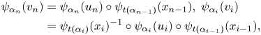
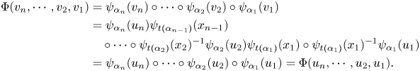
Proof. Set $\mathcal {C}=\mathcal {C}(Q,\, U)$ . For any path $p=\alpha _n\cdots \alpha _2\alpha _1$
 in $Q$
 and an element $(u_n,\, \cdots,\, u_2,\, u_1)\in U(p)$
 , we define

We claim that this is independent of the choice of the representatives; compare [Reference Li21, the proof of Proposition 2.9].
Assume that $(u_n,\, \cdots,\, u_2,\, u_1)=(v_n,\, \cdots,\, v_2,\, v_1)$ in $U(p)$
 . This means that there are elements $x_i\in U(t\alpha _i)$
 for each $1\leq i\leq n-1$
 , such that the following identities hold:

Since each $\psi _{\alpha _i}$ is a map of bisets, we have
and

Then the following identity follows immediately.
The above claim yields a well-defined functor $\Phi$ . The uniqueness of $\Phi$
 is clear, as $(u_n,\, \cdots,\, u_2,\, u_1)$
 might be viewed as the composition $u_n\circ \cdots \circ u_2\circ u_1$
 in $\mathcal {C}$
 .
.
For the ‘only if’ part of the second statement, we assume that $\Phi$ is an equivalence. Then (E1) is clear, since $\mathcal {C}$
 is free. Since $\mathcal {C}$
 is skeletal and $\Phi$
 respects isomorphism classes, (E2) follows immediately. The condition (E3) is just the denseness of $\Phi$
 . For (E4), we observe that the equivalence $\Phi$
 necessarily induces isomorphisms
of groups and bijections
between the sets of unfactorizable morphisms. Then we apply (4.2) and (4.3).
For the ‘if’ part, we assume the conditions (E1)-(E4). By (E3), the functor $\Phi$ is dense. It suffices to prove that for any $i,\, j\in Q_0$
 , the following map

is bijective.
By (E4), each $\psi _i$ is an isomorphism, and then the case $i=j$
 follows. We now assume that $i\neq j$
 . Then by (E2), $\phi (i)$
 and $\phi (j)$
 are not isomorphic.
Recall from [Reference Li21, Proposition 2.6] that each morphism in $\mathcal {D}$ has a factorization into unfactorizable morphisms. Since $\Phi$
 is dense, any morphism $g\colon \phi (i)\rightarrow \phi (j)$
 admits a factorization

with each $g_k$ unfactorizable. By (E4), each $g_k$
 belongs to the image of $\Phi$
 . It follows that there is a morphism $f\colon i\rightarrow j$
 in $\mathcal {C}$
 satisfying $\Phi (f)=g$
 . This proves that $\Phi _{i,j}$
 is surjective.
It remains to show that $\Phi _{i,j}$ is injective. Assume that $p=\alpha _n\cdots \alpha _2\alpha _1$
 and $q=\beta _m\cdots \beta _2\beta _1$
 are two paths from $i$
 to $j$
 , and that $(u_n,\, \cdots,\, u_2,\, u_1)\in U(p)$
 and $(v_m,\, \cdots,\, v_2,\, v_1)\in U(q)$
 satisfy

We claim that $p=q$ and $(u_n,\, \cdots,\, u_2,\, u_1)=(v_m,\, \cdots,\, v_2,\, v_1)$
 . Then we are done.
For the claim, we observe that the morphism $g'$ admits two factorizations:

and

Here, $i_k=t(\alpha _k)$ and $j_k=t(\beta _k)$
 . By (E4), all the morphisms appearing in the two factorizations are unfactorizable. By (E1), the EI category $\mathcal {D}$
 is free, that is, any morphism satisfies the UFP. Consequently, $m=n$
 and there are isomorphisms $g'_k\colon \phi (i_k)\rightarrow \phi (j_k)$
 making the following diagram commute.
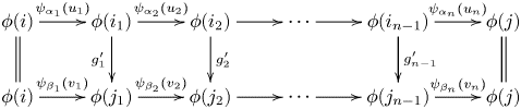
By (E2), we infer that $i_k=j_k$ ; moreover, by (E4) we obtain automorphisms $a_k\in {\rm Aut}_\mathcal {C}(i_k)=U(i_k)$
 satisfying $\psi _{i_k}(a_k)=g'_k$
 . The commutativity yields

for each $0\leq k\leq n-1$ . Here, $a_0$
 and $a_n$
 are the identity elements in $U(i)$
 and $U(j)$
 , respectively. The above identity is equivalent to

By the bijection in (E4), we infer that $\beta _{k+1}=\alpha _{k+1}$ and that
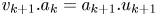
for each $0\leq k\leq n-1$ . It follows that $p=q$
 ; moreover, in view of the definition of $U(p)$
 via biset products, we infer that $(u_n,\, \cdots,\, u_2,\, u_1)=(v_n,\, \cdots,\, v_2,\, v_1)$
 , proving the claim.
4.3. $G$-actions on finite EI quivers

Let $(Q,\,U)$ be a finite EI quiver. An automorphism $\sigma =(\sigma ^0,\,\sigma ^1)$
 of $(Q,\,U)$
 consists of an automorphism $\sigma ^0\colon Q\rightarrow Q$
 of the acyclic quiver $Q$
 and an assignment $\sigma ^1=(\sigma ^1_i,\,\sigma ^1_\alpha )_{i\in Q_0, \alpha \in Q_1}$
 of isomorphisms. More precisely, for each $i\in Q_0$
 ,
,

is an isomorphism of groups; for each arrow $\alpha \in Q_1$ ,
,
is an isomorphism of $(U(t\alpha ),\, U(s\alpha ))$ -bisets. Here, the $(U(t\alpha ),\, U(s\alpha ))$
 -biset structure on $U(\sigma ^0(\alpha ))$
 is induced by the group isomorphisms $\sigma ^1_{t(\alpha )}$
 and $\sigma ^1_{s(\alpha )}$
 .
.
The composition of two automorphisms $\sigma =(\sigma ^0,\,\sigma ^1)$ and $\theta =(\theta ^0,\,\theta ^1)$
 on $(Q,\,U)$
 is given by
where the assignment $\theta ^1\star \sigma ^1$ is given by

We denote by ${\rm Aut}(Q,\,U)$ the group of automorphisms of $(Q,\,U)$
 , whose multiplication is given by the composition of automorphisms.
We observe that each automorphism $\sigma =(\sigma ^0,\, \sigma ^1)$ on $(Q,\, U)$
 induces an automorphism $\tilde {\sigma }$
 on $\mathcal {C}(Q,\, U)$
 in the following natural manner: the action of $\tilde {\sigma }$
 on objects is given by $\sigma ^0$
 ; for $u\in U(i)$
 , we have $\tilde {\sigma }(u)=\sigma ^1_i(u)\in U(\sigma ^0(i))$
 ; for a path $p=\alpha _n\cdots \alpha _2\alpha _1$
 and a morphism $(u_n,\, \cdots,\, u_2,\, u_1)\in U(p)$
 , we have

This actually gives rise to an injective group homomorphism

Let $G$ be a finite group. By a $G$
 -action on a finite EI quiver $(Q,\,U)$
 , we mean a group homomorphism

Composing $\rho$ with (4.4), the $G$
 -action makes $\mathcal {C}(Q,\, U)$
 into a $G$
 -category.
The following convention for the $G$ -action $\rho$
 will simplify the notation. For $g\in G$
 and $i\in Q_0={\rm Obj}(\mathcal {C}(Q,\,U))$
 , we write
Similarly, for $\alpha \in Q_1$ , we write $g(\alpha )=\rho (g)^0(\alpha )\in Q_1$
 . For $a\in U(i)={\rm Aut}_{\mathcal {C}(Q,\,U)}(i)$
 with $i\in Q_0$
 , we write
For $u\in U(\alpha )\subseteq {\rm Hom}^0_{\mathcal {C}(Q,\, U)}(i,\, j)$ with an arrow $\alpha \in Q_1$
 from $i$
 to $j$
 , we write
For admissible $G$ -categories, we refer to definition 2.3.
Lemma 4.3 Let $G$ be a finite group with a $G$
 -action $\rho$
 on $(Q,\, U)$
 as above. Then the corresponding $G$
 -category $\mathcal {C}(Q,\, U)$
 is admissible.
Proof. Let $g\in G$ and $i\in {\rm Obj}(\mathcal {C}(Q,\,U))=Q_0$
 such that $g(i)\neq i$
 . Recall that

Since $Q$ is acyclic, there is no path $p$
 satisfying $s(p)=g(i)$
 and $t(p)=i$
 . Therefore, the set ${\rm Hom}_{\mathcal {C}(Q,\,U)}(g(i),\,i)$
 is actually empty, proving that the $G$
 -category $\mathcal {C}(Q,\, U)$
 is admissible.
5. The quotient EI quiver
In this section, we fix a finite group $G$ and a finite EI quiver $(Q,\, U)$
 with a $G$
 -action $\rho$
 . We will construct its ‘orbifold quotient EI quiver $(\overline {Q},\, \overline {U})$
 explicitly. We prove that the free EI category $\mathcal {C}(\overline {Q},\, \overline {U})$
 is equivalent to the skew group category $\mathcal {C}(Q,\, U)\rtimes G$
 ; see theorem 5.3.
For each vertex $i$ and each arrow $\alpha$
 in $Q$
 , their stabilizers are denoted by $G_i$
 and $G_\alpha$
 , respectively. We observe that $G_\alpha \subseteq G_{s(\alpha )}\cap G_{t(\alpha )}$
 .
.
5.1. The construction of $(\overline {Q},\, \overline {U})$

The finite quiver $\overline {Q}=(\overline {Q}_0,\, \overline {Q}_1; s,\, t)$ is just the quotient quiver of $Q$
 by $G$
 . In more details, $\overline {Q}_0=Q_0/G$
 and $\overline {Q}_1=Q_1/G$
 are the corresponding sets of $G$
 -orbits, and the maps $s$
 and $t$
 are induced by the ones of $Q$
 . Since $Q$
 is acyclic, we infer that the finite quiver $\overline {Q}$
 is acyclic. By definition, we have the canonical projections

The vertices and arrows in $\overline {Q}$ are written in the bold form. For example, the vertices are usually denoted by $\boldsymbol {i}$
 and $\boldsymbol {j}$
 .
.
To define the assignment $\overline {U}$ , we have to fix three maps

satisfying the following conditions: $\pi _0\circ \iota _0={\rm Id}_{\overline {Q}_0}$ , $\pi _1\circ \iota _1={\rm Id}_{\overline {Q}_1}$
 ,
,

for each arrow $\boldsymbol {\alpha }\in \overline {Q}_1$ . Here, we use the convention (4.5) for $g_{\boldsymbol {\alpha }}(\iota _0(s\boldsymbol {\alpha }))$
 .
.
The inclusion $G_{\iota _1(\boldsymbol {\alpha })}\subseteq G_{\iota _0(t\boldsymbol {\alpha })}$ makes $G_{\iota _0(t\boldsymbol {\alpha })}$
 a right $G_{\iota _1(\boldsymbol {\alpha })}$
 -set. The injective group homomorphism

makes $G_{\iota _0(s\boldsymbol {\alpha })}$ a left $G_{\iota _1(\boldsymbol {\alpha })}$
 -set. Therefore, we have the biset product

which is naturally a $(G_{\iota _0(t\boldsymbol {\alpha })},\,G_{\iota _0(s\boldsymbol {\alpha })})$ -biset. A typical element in the above biset product is written as $(h,\, g)$
 with $h\in G_{\iota _0(t\boldsymbol {\alpha })}$
 and $g\in G_{\iota _0(s\boldsymbol {\alpha })}$
 . By definition, we have
for each $k\in G_{\iota _1(\boldsymbol {\alpha })}$ .
.
Finally, we choose a right coset decomposition

Consequently, any element in $G_{\iota _0(t\boldsymbol {\alpha })} \times _{G_{\iota _1(\boldsymbol {\alpha })}} G_{\iota _0(s\boldsymbol {\alpha })}$ is uniquely written as $(h_{\boldsymbol {\alpha },\, r},\,k)$
 for $1\leq r\leq m_{\boldsymbol {\alpha }}$
 and $k\in G_{\iota _0(s\boldsymbol {\alpha })}$
 .
.
The construction of the assignment $\overline {U}$ is as follows. For each vertex $\boldsymbol {i}$
 of $\overline {Q}$
 , we set
Here, we note that $G_{\iota _0(\boldsymbol {i})}$ acts on $U(\iota _0(\boldsymbol {i}))$
 by group automorphisms. Therefore, the semi-direct product is well defined. For each arrow $\boldsymbol {\alpha }\colon \boldsymbol {i}\rightarrow \boldsymbol {j}$
 in $\overline {Q}$
 , we set
A typical element in $\overline {U}(\boldsymbol {\alpha })$ is denoted by $(u,\, (h_{\boldsymbol {\alpha },\, r},\, k))$
 . The right $\overline {U}(\boldsymbol {i})$
 -action is given by

for any $(a,\, g)\in \overline {U}(\boldsymbol {i})=U(\iota _0(\boldsymbol {i}))\rtimes G_{\iota _0(\boldsymbol {i})}$ . Here, using the convention (4.6), we observe that $g_{\boldsymbol {\alpha }}k(a)$
 lies in $U(g_{\boldsymbol {\alpha }} \iota _0(\boldsymbol {i}))=U(s\iota _1(\boldsymbol {\alpha }))$
 , and that $u.(g_{\boldsymbol {\alpha }}k(a))$
 means the right $U(s\iota _1(\boldsymbol {\alpha }))$
 -action on $U(\iota _1(\boldsymbol {\alpha }))$
 .
.
To describe the left $\overline {U}(\boldsymbol {j})$ -action, we take an arbitrary element $(b,\, h)\in \overline {U}(\boldsymbol {j})=U(\iota _0(\boldsymbol {j}))\rtimes G_{\iota _0(\boldsymbol {j})}$
 . Assume that
for some $1\leq p\leq m_{\boldsymbol {\alpha }}$ and $k'\in G_{\iota _1(\boldsymbol {\alpha })}$
 . The left $\overline {U}(\boldsymbol {j})$
 -action is given by
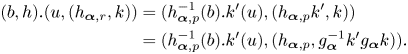
Here, we observe that $h^{-1}_{\boldsymbol {\alpha },\, p}(b)$ lies in $U(\iota _0(\boldsymbol {j}))=U(t\iota _1(\boldsymbol {\alpha }))$
 , and that $k'(u)$
 lies in $U(\iota _1(\boldsymbol {\alpha }))$
 . The convention (4.7) is used for $k'(u)$
 . Finally, $h^{-1}_{\boldsymbol {\alpha },\, p}(b).k'(u)$
 denotes the left $U(t\iota _1(\boldsymbol {\alpha }))$
 -action on $U(\iota _1(\boldsymbol {\alpha }))$
 .
.
The above actions make $\overline {U}(\boldsymbol {\alpha })$ a $(\overline {U}(\boldsymbol {j}),\, \overline {U}(\boldsymbol {i}))$
 -biset. In summary, we have defined the finite EI quiver $(\overline {Q},\, \overline {U})$
 .
.
The above construction of the quotient EI quiver $(\overline {Q},\, \overline {U})$ is rather general. In what follows, we impose conditions which will simplify the construction.
Remark 5.1 Assume that the $G$ -action $\rho$
 on $(Q,\, U)$
 satisfies the following triviality conditions:
(1) for each $i\in Q_0$
, $g\in G_i$ and $a\in U(i)$, we have $g(a)=a$;(2) for each $\alpha \in Q_1$
, $g\in G_\alpha$ and $u\in U(\alpha )$, we have $g(u)=u$.


Then the quotient EI quiver $(\overline {Q},\, \overline {U})$ is described as follows:
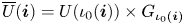
is the direct product; for each arrow $\boldsymbol {\alpha }\colon \boldsymbol {i}\rightarrow \boldsymbol {j}$ in $\overline {Q}$
 , we have

Its typical element is denoted by $(u,\, (h,\, k))$ for $u\in U(\iota _1(\boldsymbol {\alpha }))$
 , $h\in G_{\iota _0(\boldsymbol {j})}$
 and $k\in G_{\iota _0(\boldsymbol {i})}$
 . The right $\overline {U}(\boldsymbol {i})$
 -action is given by

The left $\overline {U}(\boldsymbol {j})$ -action is given by

Here, $u.g_{\boldsymbol {\alpha }}(a)$ and $b.u$
 mean the right $U(s\iota _1(\boldsymbol {\alpha }))$
 -action and the left $U(t\iota _1(\boldsymbol {\alpha }))$
 -action on $U(\iota _1(\boldsymbol {\alpha }))$
 , respectively.
The group action in the following example does not satisfy the triviality condition (1) in remark 5.1.
Example 5.2 Let $Q$ be the following Kronecker quiver.

We endow it with the following assignment $U$ : for each vertex $i=1,\, 2$
 , we set

to be a cyclic group of order $3$ generated by $a_i$
 ; for each arrow $\alpha _i$
 , we set $U(\alpha _i)=\{u_i\}$
 to be a trivial $(U(2),\,U(1))$
 -biset with a single element.
Let $G=\{1_G,\, g\}$ be a cyclic group of order $2$
 . We define a $G$
 -action on the EI quiver $(Q,\, U)$
 as follows: $g$
 acts on $Q$
 by interchanging the arrows $\alpha _1$
 and $\alpha _2$
 ; its action on the assignment $U$
 is given by

The quotient quiver $\overline {Q}$ is of type $A_2$
 .
.
To describe the assignment $\overline {U}$ on $\overline {Q}$
 , we set $\iota _1({\boldsymbol {\alpha }})=\alpha _1$
 and $g_{\boldsymbol {\alpha }}=1_G$
 . The stabilizers are given by $G_{\alpha _1}=\{1_G\}$
 and $G_1=G=G_2$
 . Therefore, we have

We observe that $\overline {U}(\boldsymbol {1})$ is isomorphic to the symmetric group $S_3$
 , and that $\overline {U}(\boldsymbol {2})$
 is isomorphic to a cyclic group of order $6$
 . For the unique arrow $\boldsymbol {\alpha }$
 , we have

as a set. The left $\overline {U}(\boldsymbol {2})$ -action on $\overline {U}(\boldsymbol {\alpha })$
 is give by

for any $0\leq m\leq 2$ , $0\leq n\leq 1$
 and $(x,\,y)\in G\times G$
 . The right $\overline {U}(\boldsymbol {1})$
 -action on $\overline {U}(\boldsymbol {\alpha })$
 is given by
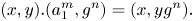
5.2. An equivalence of categories
The EI quiver $(\overline {Q},\, \overline {U})$ might be viewed as a certain ‘orbifold’ quotient of $(Q,\, U)$
 . We mention a similar construction in the classic work [Reference Bass2, Section 3] on graphs of groups. The EI quiver $(\overline {Q},\, \overline {U})$
 depends on the choices in (5.1) and (5.4).
The following result justifies the quotient construction.
Theorem 5.3 Let $(Q,\, U)$ be a finite EI quiver with a $G$
 -action $\rho$
 , and let $(\overline {Q},\, \overline {U})$
 be its quotient as above. Then there is an equivalence of categories

Proof. We write $\mathcal {C}=\mathcal {C}(Q,\, U)$ in this proof. We will apply proposition 4.2 to deduce the equivalence. We use the map $\iota _0\colon \overline {Q}_0\rightarrow Q_0={\rm Obj}(\mathcal {C}\rtimes G)$
 , and the identification

where the right equality follows by combining lemma 4.3 and corollary 2.6.
To apply proposition 4.2, it remains to construct for each arrow $\boldsymbol {\alpha }$ in $\overline {Q}$
 , a map between bisets

We will see in the following construction that these maps between bisets yield the required bijection in (E4).
By corollary 3.4, the category $\mathcal {C}\rtimes G$ is EI free, therefore the condition (E1) is satisfied. For two different vertices $\boldsymbol {i}$
 and $\boldsymbol {j}$
 , the vertices $\iota _0(\boldsymbol {i})$
 and $\iota _0(\boldsymbol {j})$
 are not in the same $G$
 -orbit. By lemma 2.2(2), $\iota _0(\boldsymbol {i})$
 and $\iota _0(\boldsymbol {j})$
 are not isomorphic in $\mathcal {C}\rtimes G$
 , proving the condition (E2). For each vertex $i\in Q_0$
 , the corresponding object $i$
 is isomorphic to $\iota _0(\pi _0(i))$
 in $\mathcal {C}\rtimes G$
 , proving (E3). Once we construct the above maps between bisets, we will infer by proposition 4.2 the required equivalence of categories.
To construct the required maps, we take arbitrary vertices $\boldsymbol {i}$ and $\boldsymbol {j}$
 in $\overline {Q}$
 . By lemma 3.2, we have
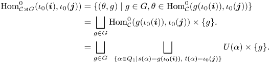
Here, for the last equality we use (4.3).
For each arrow $\boldsymbol {\alpha }\colon \boldsymbol {i}\rightarrow \boldsymbol {j}$ , we define the following subset of ${\rm Hom}^0_{\mathcal {C}\rtimes G}(\iota _0(\boldsymbol {i}),\,\iota _0(\boldsymbol {j}))$

Recall from example 4.1 that the $(\overline {U}(\boldsymbol {j}),\, \overline {U}(\boldsymbol {i}))$ -biset structure on ${\rm Hom}^0_{\mathcal {C}\rtimes G}(\iota _0(\boldsymbol {i}), \iota _0(\boldsymbol {j}))$
 is induced by composition (2.1) of morphisms in $\mathcal {C}\rtimes G$
 . Then we infer that $S(\boldsymbol {\alpha })$
 is a $(\overline {U}(\boldsymbol {j}),\, \overline {U}(\boldsymbol {i}))$
 -sub-biset. Now, we have the following disjoint union
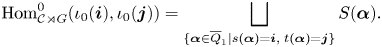
We will complete the proof by establishing an isomorphism of $(\overline {U}(\boldsymbol {j}),\, \overline {U}(\boldsymbol {i}))$ -bisets
for any arrow $\boldsymbol {\alpha }\colon \boldsymbol {i}\rightarrow \boldsymbol {j}$ . Indeed, in view of (5.5), the isomorphism yields the required bijection in (E4). Then we are done.
To analyse $S(\boldsymbol {\alpha })$ , we observe that in the index set of the outer disjoint union, the arrows $\alpha$
 are of the form $h(\iota _1(\boldsymbol {\alpha }))$
 for some $h\in G_{\iota _0(\boldsymbol {j})}$
 . By the coset decomposition (5.4), there is a unique $1\leq r\leq m_{\boldsymbol {\alpha }}$
 satisfying
For simplicity, we write $h_r$ for $h_{\boldsymbol {\alpha },\, r}$
 . In the inner disjoint union, we have

Consequently, there is a unique $k\in G_{\iota _0(\boldsymbol {i})}$ satisfying

The above analysis implies that

We observe that $U(\iota _1(\boldsymbol {\alpha }))$ is bijective to each $U(h_r(\iota _1(\boldsymbol {\alpha })))$
 via $\rho (h_r)^1_{\iota _1(\boldsymbol {\alpha })}$
 , which sends $u\in U(\iota _1(\boldsymbol {\alpha }))$
 to $h_r(u)\in U(h_r(\iota _1(\boldsymbol {\alpha })))$
 . Moreover, the biset product

is bijective to
which is further bijective to the following disjoint union
Using these bijections, we infer that the following map

is a bijection. We omit the routine verification that this explicit bijection is indeed a map of $(\overline {U}(\boldsymbol {j}),\, \overline {U}(\boldsymbol {i}))$ -bisets. This is the required isomorphism of bisets.
Let $\Delta =(\Delta _0,\, \Delta _1; s,\, t)$ be a finite acyclic quiver. Recall that the path category $\mathcal {P}_\Delta$
 is defined as follows: ${\rm Obj}(\mathcal {P}_\Delta )=\Delta _0$
 and ${\rm Hom}_{\mathcal {P}_\Delta }(i,\, j)$
 consists of all paths from $i$
 to $j$
 ; the composition is given by concatenation of paths.
Denote by $(\Delta,\, U_{\rm tr})$ the EI quiver with trivial assignment $U_{\rm tr}$
 , that is, each group $U_{\rm tr}(i)$
 is trivial and each biset $U_{\rm tr}(\alpha )$
 has only one element. We observe

Let $G$ be a finite group which acts on $\Delta$
 by quiver automorphisms. Then $G$
 acts on the associated EI quiver $(\Delta,\, U_{\rm tr})$
 . Denote by $(\overline {\Delta },\, \overline {U}_{\rm tr})$
 the quotient EI quiver. Therefore, $\overline {\Delta }$
 is the quotient quiver of $\Delta$
 by $G$
 . Fix the choices (5.1). In view of remark 5.1, the assignment $\overline {U}_{\rm tr}$
 is described as follows: for each vertex $\boldsymbol {i}$
 of $\overline {\Delta }$
 , we have
for each arrow $\boldsymbol {\alpha }\colon \boldsymbol {i}\rightarrow \boldsymbol {j}$ in $\overline {\Delta }$
 , we have
whose $(G_{\iota _0(\boldsymbol {i})},\, G_{\iota _0(\boldsymbol {j})})$ -biset structure is given by the multiplication of $G_{\iota _0(\boldsymbol {i})}$
 from the left, and of $G_{\iota _0(\boldsymbol {j})})$
 from the right.
In view of (5.6), we have the following special case of theorem 5.3.
Corollary 5.4 Let $\Delta$ be a finite acyclic quiver with a $G$
 -action. Keep the notation as above. Then there is an equivalence of categories
6. Categories and algebras associated to Cartan triples
In this section, we will first recall the algebras [Reference Geiss, Leclerc and Schröer11] and EI categories [Reference Chen and Wang4] associated to Cartan triples. For an action of a finite group on a finite acyclic quiver, we give sufficient conditions on when the quotient EI quiver is of Cartan type. Consequently, the skew group algebra of the path algebra is Morita equivalent to the algebra studied in [Reference Geiss, Leclerc and Schröer11]; see theorem 6.6.
For two nonzero integers $a$ and $b$
 , we denote by ${\rm gcd}(a,\,b)$
 their greatest common divisor, which is always assumed to be positive.
6.1. Cartan triples
Let $n\geq 1$ be a positive integer. An $n\times n$
 matrix $C=(c_{ij})$
 with integer coefficients is called a symmetrizable generalized Cartan matrix, provided that the following conditions are satisfied:
(C1) $c_{ii}=2$
for all $i$;(C2) $c_{ij}\leq 0$
for all $i\neq j$, and $c_{ij}<0$ if and only if $c_{ji}<0$;(C3) There is a diagonal matrix $D={\rm diag}(c_1,\,\cdots,\,c_n)$
with $c_i\in \mathbb {Z}_{\geq 1}$ for all $i$ such that the product matrix $DC$ is symmetric.


The matrix $D$ appearing in (C3) is called a symmetrizer of $C$
 . For brevity, a symmetrizable generalized Cartan matrix is called a Cartan matrix.
Let $C=(c_{ij})$ be a Cartan matrix. An (acyclic) orientation of $C$
 is a subset $\Omega \subset \{1,\,2,\,\cdots,\,n\}\times \{1,\,2,\,\cdots,\,n\}$
 such that the following conditions are satisfied:
(O1) $\{(i,\,j),\,(j,\,i)\}\cap \Omega \neq \emptyset$
if and only if $c_{ij}<0$;(O2) for each sequence $((i_1,\,i_2),\,(i_2,\,i_3),\,\cdots,\,(i_t,\,i_{t+1}))$
with $t\geq 1$ and $(i_s,\,i_{s+1})\in \Omega$ for all $1\leq s\leq t$, we have $i_1\neq i_{t+1}$.


Following [Reference Chen and Wang4], we will call $(C,\, D,\, \Omega )$ a Cartan triple, where $C$
 is a Cartan matrix, $D$
 its symmetrizer and $\Omega$
 an orientation of $C$
 .
.
In what follows, we recall that, associated to each Cartan triple, there are a finite free EI category $\mathcal {C}(C,\, D,\, \Omega )$ and a finite dimensional algebra $H(C,\, D,\, \Omega )$
 .
.
Let $Q=Q(C,\,\Omega )$ be the finite quiver with the set of vertices $Q_0=\{1,\,2,\, \cdots,\,n\}$
 and with the set of arrows

Let $Q^{\circ }=Q^{\circ }(C,\,\Omega )$ be the quiver obtained from $Q$
 by deleting all the loops $\varepsilon _i$
 . By the condition (O2), we infer that the finite quiver $Q^{\circ }$
 is acyclic.
We recall the finite EI quiver $(Q^\circ,\, X)$ . The assignment $X$
 is given as follows: $X(i)=\langle \eta _i\; |\; \eta _i^{c_i}=1\rangle$
 is a cyclic group of order $c_i$
 ; for each $(i,\, j)\in \Omega$
 , we set $G_{ij}=\langle \eta _{ij}\; |\; \eta _{ij}^{{\rm gcd}(c_i,\, c_j)}=1\rangle$
 to be a cyclic group of order ${\rm gcd}(c_i,\, c_j)$
 . There are injective group homomorphisms
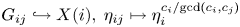
and
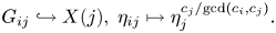
Then we have the $(X(i),\, X(j))$ -biset $X(i)\times _{G_{ij}} X(j)$
 . We set
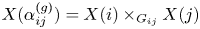
for each $1\leq g\leq {\rm gcd}(c_{ij},\, c_{ji})$ .
.
Definition 6.1 [Reference Chen and Wang4, Definition 4.1]
Associated to a Cartan triple $(C,\, D,\, \Omega )$ , the finite EI category $\mathcal {C}(C,\, D,\, \Omega )$
 is defined to be the free EI category $\mathcal {C}(Q^\circ,\, X)$
 associated to the above EI quiver $(Q^\circ,\, X)$
 . We say that such EI quivers $(Q^\circ,\, X)$
 and EI categories $\mathcal {C}(C,\, D,\, \Omega )$
 are both of Cartan type.
Let $\mathbb {K}$ be a field. The following algebras [Reference Geiss, Leclerc and Schröer11] play a fundamental role in categorifying the root lattices for non-symmetric Caran matrices. For more background, we refer to [Reference Geiss10].
Definition 6.2 [Reference Geiss, Leclerc and Schröer11, Section 1.4]
Let $(C,\, D,\, \Omega )$ be a Cartan triple with $Q=Q(C,\,\Omega )$
 . Consider the following $\mathbb {K}$
 -algebra
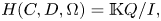
where $\mathbb {K}Q$ is the path algebra of $Q$
 , and $I$
 is the two-sided ideal of $\mathbb {K}Q$
 generated by the following set
We will recall from [Reference Chen and Wang4, Subsection 4.2] the construction of a new Cartan triple $(C',\, D',\, \Omega ')$ from a given one $(C,\, D,\, \Omega )$
 , which depends on the characteristic of $\mathbb {K}$
 . Recall that $D={\rm diag}(c_1,\, \cdots,\, c_n)$
 .
.
Construction $(\dagger )$ for the case ${\rm char}(\mathbb {K})=p>0$
 . Assume that $c_i=p^{r_i}d_i$
 satisfying $r_i\geq 0$
 and ${\rm gcd}(p,\, d_i)=1$
 . For each $1\leq i,\, j\leq n$
 , we set

The rows and columns of the Cartan matrix $C'$ and its symmetrizer $D'$
 are indexed by the following set
The diagonal entries of $C'$ are $2$
 , and the off-diagonal entries are given as follows:
Let $D'$ be a diagonal matrix, whose $(i,\, l_i)$
 -th component is given by $p^{r_i}$
 . Set
. Set

which is an orientation of $C'$ .
.
Construction $(\dagger )$ for the case ${\rm char}(\mathbb {K})=0$
 . This is very similar to the above construction. We put $d_i=c_i$
 and replace $\Sigma _{ij}^p$
 by
by

The off-diagonal entries of $C'$ is given by
We observe that $C'$ is symmetric and that $D'$
 is the identity matrix.
We say that $\mathbb {K}$ has enough roots of unity for $D$
 , if for each $1\leq i\leq n$
 , the polynomial $t^{c_i}-1$
 splits in $\mathbb {K}[t]$
 .
.
Theorem 6.3 Assume that $(C,\, D,\, \Omega )$ is a Cartan triple and that $\mathbb {K}$
 has enough roots of unity for $D$
 . Keep the notation in Construction $(\dagger )$
 . Then there is an isomorphism of algebras

Proof. This result is due to [Reference Chen and Wang4, Theorem 4.3]. We mention that the assumption here on $\mathbb {K}$ is slightly weaker than the one therein. Since each polynomial $t^{c_i}-1$
 splits, we infer that, in Construction $(\dagger )$
 for each case, the ground field $\mathbb {K}$
 has a $(\prod _{i=1}^n d_i)$
 -th primitive root of unity. Then the proof of [Reference Chen and Wang4, Theorem 4.3], in particular, the argument in [Reference Chen and Wang4, Section 5], carries through under the weaker assumption here.
We are mainly interested in the following special case.
Proposition 6.4 Assume that ${\rm char}(\mathbb {K})=p>0$ and that $(C,\, D,\, \Omega )$
 is a Cartan triple such that each $c_i$
 is a $p$
 -power. Then there is an isomorphism of algebras
which identifies ${\rm Span}_\mathbb {K}\{{\rm Id}_i,\, \eta _i,\, \cdots,\, \eta _i^{c_i-1}\}$ with ${\rm Span}_\mathbb {K}\{e_i,\, \varepsilon _{i},\, \cdots,\, \varepsilon _{i}^{c_i-1}\}$
 .
.
Here, ${\rm Span}_\mathbb {K}$ means the subspace spanned by the mentioned elements. Both ${\rm Id}_i$
 and $\eta _i$
 are viewed as automorphisms of $i$
 in $\mathcal {C}(C,\, D,\, \Omega )$
 . Similarly, the trivial path $e_i$
 and the loop $\varepsilon _i$
 are viewed as elements in $H(C,\, D,\, \Omega )$
 .
.
Proof. The assumption on entries of $D$ implies that $(C',\, D',\, \Omega ')=(C,\, D,\, \Omega )$
 , where we identify $(i,\, 0)\in M$
 with $i$
 ; see [Reference Chen and Wang4, Example 6.7]. For the same reason, the polynomials $t^{c_i}-1$
 splits, that is, $\mathbb {K}$
 has enough roots of unity for $D$
 . Then the isomorphism follows from theorem 6.3. By the proof of [Reference Chen and Wang4, Theorem 4.3], the isomorphism clearly identifies the above two subspaces.
Remark 6.5 In general, the isomorphism in proposition 6.4 is not explicitly given. However, from the proof in [Reference Chen and Wang4, Theorem 4.3], we infer that the isomorphism sends ${\rm Id}_i$ to $e_i$
 , and sends $\eta _i$
 to $e_i+\varepsilon _i$
 .
.
6.2. From quotient to Cartan type
We study the situation of corollary 5.4. Let $G$ be a finite group and let $\Delta$
 be a finite acyclic quiver with a $G$
 -action. We give conditions on when the quotient EI quiver $(\overline {\Delta },\, \overline {U}_{\rm tr})$
 is of Cartan type.
The following natural conditions will be imposed on the quiver $\Delta$ .
.
(1) For each $i$
, the stabilizer $G_i=\langle \xi _i\mid \xi _i^{a_i}=1\rangle$ is cyclic with order $a_i$.(2) For each arrow $\alpha \colon i\rightarrow j$
, we have that $\xi _i^{{a_i}/{{\rm gcd}(a_i,\,a_j)}}=\xi _j^{{a_j}/{{\rm gcd}(a_i,\,a_j)}}$ and both belong to $G_\alpha$.(3) For each $g\in G$
, we have $\xi _{g(i)}=g\xi _ig^{-1}$.


The condition (${\dagger} 3$ ) means that the choice of the specific generators $\xi _i$
 for $G_i$
 is compatible with the $G$
 -action. It follows from (${\dagger} 2$
 ) that the inclusion $G_\alpha \subseteq G_i\cap G_j$
 is an equality.
Associated to the $G$ -action on $\Delta$
 , we will define a Cartan triple $(C,\, D,\, \Omega )$
 ; compare [Reference Lusztig23, Section 14.1]. The rows and columns of $C$
 and $D$
 are indexed by the orbit set $\overline {\Delta }_0=\Delta _0/G$
 . For each $G$
 -orbit $\boldsymbol {i}$
 of vertices, the corresponding diagonal entry of $D$
 is
is

where $|\boldsymbol {i}|$ denotes the cardinality of the $G$
 -orbit. For any vertices $\boldsymbol {i}$
 and $\boldsymbol {j}$
 , we denote by $N_{\boldsymbol {i},\, \boldsymbol {j}}$
 the number of arrows in $\Delta$
 between the $G$
 -orbit $\boldsymbol {i}$
 and $G$
 -orbit $\boldsymbol {j}$
 . The corresponding off-diagonal entry of $C$
 is given by
The orientation $\Omega$ is consistent with that of $\overline {\Delta }$
 , that is, $(\boldsymbol {j},\, \boldsymbol {i})\in \Omega$
 if and only if there is an arrow from $\boldsymbol {i}$
 to $\boldsymbol {j}$
 in $\overline {\Delta }$
 .
.
By the equality $c_{\boldsymbol {i}}c_{\boldsymbol {i},\, \boldsymbol {j}}=c_{\boldsymbol {j}}c_{\boldsymbol {j},\, \boldsymbol {i}}$ , we infer the following useful identity
Theorem 6.6 Assume that the $G$ -action on $\Delta$
 satisfies $({\dagger} 1)\mbox {-}({\dagger} 3)$
 and that the associated Cartan triple is $(C,\, D,\, \Omega )$
 . Denote by $(Q^\circ,\, X)$
 the corresponding EI quiver of Cartan type. Then there is an isomorphism of EI quivers
Moreover, we have the following immediate consequences.
(1) There is an equivalence of categories
\[ \mathcal{P}_\Delta\rtimes G\simeq \mathcal{C}(C, D, \Omega). \]
(2) Assume that $\mathbb {K}$
has enough roots of unity for $D$ and that the Cartan triple $(C',\, D',\, \Omega ')$ is given in Construction $(\dagger )$. Then the algebras $\mathbb {K}\Delta \# G$ and $H(C',\, D',\, \Omega ')$ are Morita equivalent.(3) Assume that ${\rm char}(\mathbb {K})=p>0$
and that $G$ is a $p$-group. Then the algebras $\mathbb {K}\Delta \# G$ and $H(C,\, D,\, \Omega )$ are Morita equivalent.


Proof. We first prove the isomorphism of EI quivers. Take two vertices $\boldsymbol {i}=Gi$ and $\boldsymbol {j}=Gj$
 in $\overline {\Delta }$
 . We observe $c_{\boldsymbol {i}}=a_i$
 and $c_{\boldsymbol {j}}=a_j$
 . For each arrow $\alpha$
 between $i$
 and $j$
 in $\Delta$
 , we have observed that $G_\alpha =G_i\cap G_j$
 , which is of order ${\rm gcd}(|G_i|,\, |G_j|)$
 . Then we have
It follows that the number of arrows between $\boldsymbol {i}$ and $\boldsymbol {j}$
 in $\overline {\Delta }$
 equals
Here, the last equality uses (6.2). Recall that the vertex set of $Q^\circ$ is bijective to the index set of rows of $C$
 , namely the vertex set $\overline {\Delta }_0$
 . By comparing the number of arrows, we identify $\overline {\Delta }$
 with $Q^\circ$
 .
.
We now compare the assignments $\overline {U}_{\rm tr}$ and $X$
 . By (${\dagger} 1$
 ), we infer that $\overline {U}_{\rm tr}(\boldsymbol {i})=G_{\iota _0(\boldsymbol {i})}$
 is cyclic of order $c_{\boldsymbol {i}}=a_i$
 . For each arrow $\boldsymbol {\alpha }\colon \boldsymbol {i}\rightarrow \boldsymbol {j}$
 in $\overline {\Delta }$
 , we write $\iota _0(\boldsymbol {i})=i$
 and $\iota _0(\boldsymbol {j})=j$
 . By (5.2), we have the arrow $\iota _1(\boldsymbol {\alpha })\colon g_{\boldsymbol {\alpha }}(i)\rightarrow j$
 in $\Delta$
 . By (${\dagger} 2$
 ) and (${\dagger} 3$
 ), we have
Recall that $\overline {U}_{\rm tr}(\boldsymbol {\alpha })=G_i\times _{G_{\iota _1(\boldsymbol {\alpha })}}G_j$ . In view of (5.3), the above identity implies that, in $\overline {U}_{\rm tr}(\boldsymbol {\alpha })$
 , we have
This actually implies that the following map is well defined

The above map is bijective and respects the $(G_i,\, G_j)$ -biset structures. We readily deduce that the assignment $\overline {U}_{\rm tr}$
 is isomorphic to $X$
 , as required.
For (1), we recall that $\mathcal {C}(C,\, D,\, \Omega )=\mathcal {C}(Q^\circ,\, X)$ . Then the equivalence of categories follows from the obtained isomorphism of EI quivers and corollary 5.4.
For (2) and (3), we recall that the path algebra $\mathbb {K}\Delta$ is identified with the category algebra $\mathbb {K}\mathcal {P}_\Delta$
 of the path category. By proposition 2.1, we identify $\mathbb {K}(\mathcal {P}_\Delta \rtimes G)$
 with $\mathbb {K}\mathcal {P}_\Delta \# G$
 . Recall from [Reference Webb32, Proposition 2.2] that the category algebras of two equivalent categories are Morita equivalent. Applying (1), we infer that $\mathbb {K}\mathcal {C}(C,\, D,\, \Omega )$
 and $\mathbb {K}(\mathcal {P}_\Delta \rtimes G)$
 are Morita equivalent. In summary, we have obtained that $\mathbb {K}\mathcal {C}(C,\, D,\, \Omega )$
 and $\mathbb {K}\Delta \# G$
 are Morita equivalent.
Now, the required statement in (2) follows from the isomorphism in theorem 6.3. For (3), we observe that each $c_{\boldsymbol {i}}$ is a $p$
 -power, as $G$
 is a $p$
 -group. We apply the isomorphism in proposition 6.4.
Although the conditions $({\dagger} 1)\mbox {-}({\dagger} 3)$ are technical, as we will see, natural examples are ubiquitous. The following construction is inspired by [Reference Serre27, Section 5.3].
Example 6.7 Let $n\geq 1$ and $G$
 be a finite group. For each $1\leq i\leq n$
 , we fix $\xi _i\in G$
 and assume that $\xi _i$
 is of order $a_i$
 . The cyclic subgroup generated by $\xi _i$
 is denoted by $H_i$
 . The elements $\xi _i$
 may not be distinct. Denote by $G/{H_i}$
 the set of left $H_i$
 -cosets, whose elements are denoted by $gH_i$
 .
.
We construct an acyclic quiver $\Delta$ as follows: the set $\Delta _0$
 of vertices is a disjoint union $\bigsqcup _{i=1}^n G/{H_i}\times \{i\}$
 ; only if $i< j$
 and $\xi _i^{{a_i}/{{\rm gcd}(a_i,\,a_j)}}=\xi _j^{{a_j}/{{\rm gcd}(a_i,\,a_j)}}$
 , each coset $g(H_i\cap H_j)$
 is viewed as an arrow starting at $(gH_i,\, i)$
 and terminating at $(gH_j,\, j)$
 . The natural action of $G$
 on left cosets induces a $G$
 -action on $\Delta$
 . It is trivial to verify that $({\dagger} 1)\mbox {-}({\dagger} 3)$
 do hold for the $G$
 -action.
The following example is our main concern.
Example 6.8 Let $G=\langle \xi \mid \xi ^a=1\rangle$ be a cyclic group of order $a$
 . Assume that $G$
 acts on $\Delta$
 such that $G_\alpha =G_{s(\alpha )}\cap G_{t(\alpha )}$
 for each arrow $\alpha$
 in $\Delta$
 . Then the conditions $({\dagger} 1)\mbox {-}({\dagger} 3)$
 are satisfied.
For each vertex $i$ with $|G_{i}|=a_i$
 , we take the generator $\xi _i$
 to be $\xi ^{{a}/{a_i}}$
 . Then it is direct to check that $({\dagger} 1)\mbox {-}({\dagger} 3)$
 hold.
hold.
Remark 6.9 We observe that any Cartan triple does arise in the situation of example 6.8. More precisely, given any Cartan triple $(C,\, D,\, \Omega )$ , we will construct an acyclic quiver with a cyclic group action such that its associated Cartan triple is the given one; compare [Reference Lusztig23, Section 14.1].
Assume that $c={\rm lcm}(c_1,\, c_2,\, \cdots,\, c_n)$ is the least common multiple of the entries of $D$
 . Set $d_i={c}/{c_i}$
 . We construct an acyclic quiver $\Delta$
 as follows. The vertex set and arrow set are given by

and

respectively, where $\Sigma _{ij}$ is defined in (6.1). We observe the following identity
Let $G=\langle \sigma \mid \sigma ^c=1\rangle$ be a cyclic group of order $c$
 . Then $G$
 acts on $\Delta$
 such that

Here, we identify $(i,\, d_i)$ with $(i,\, 0)$
 . This defines a $G$
 -action on $\Delta$
 . It is clear that $G_\alpha =G_{s(\alpha )}\cap G_{t(\alpha )}$
 for each arrow $\alpha$
 in $\Delta$
 . Then by example 6.8, theorem 6.6 applies to this $G$
 -action. Moreover, the associated Cartan triple coincides with the given one.
The following counter-example shows that the condition $G_{\alpha }=G_{s(\alpha )}\cap G_{t(\alpha )}$ in example 6.8 is necessary.
Example 6.10 Let $\Delta$ be the following Kronecker quiver.

Let $G=\{1_G,\, \xi \}$ be a cyclic group of order $2$
 which acts on $\Delta$
 by interchanging $\alpha$
 and $\beta$
 . We observe that $G_{\alpha }=G_\beta =\{1_G\}\subsetneq G_1\cap G_2=G$
 . It follows that $({\dagger} 2)$
 is not satisfied.
The quotient quiver $\overline {\Delta }$ is of type $A_2$
 .
.
The assignment $\overline {U}_{\rm tr}$ is described as follows: $\overline {U}_{\rm tr}(\boldsymbol {1})=G=\overline {U}_{\rm tr}(\boldsymbol {2})$
 , and
, and
The quotient EI quiver $(\overline {\Delta },\, \overline {U}_{\rm tr})$ is not of Cartan type.
7. Induced modules and folding
In this final section, we first study induced modules on a skew group algebra. For a finite cyclic group action on a finite acyclic quiver, the main goal of the paper, theorem 7.8, constructs a categorification of the folding projection between the relevant root lattices. In the Dynkin cases, the restriction of the categorification to indecomposable modules corresponds to the folding of positive roots; see proposition 7.9.
7.1. Generalities on induced modules
Let $A$ be a finite dimensional $\mathbb {K}$
 -algebra, and let $G$
 be a finite group acting on $A$
 by algebra automorphisms. Denote by $A\# G$
 the skew group algebra. We view $A$
 as a subalgebra of $A\# G$
 by identifying $a\in A$
 with $a\#1_G\in A\#G$
 .
.
For a left $A$ -module $M$
 , we define a left $A\#G$
 -module $M\#G$
 , the induced module, as follows: $M\#G=M\otimes \mathbb {K}G$
 as a vector space, and its left $A\#G$
 -action is given by

for any $a\#g\in A\#G$ and $m\#h\in M\#G$
 . There is an isomorphism of left $A\# G$
 -modules

Similarly, for a right $A$ -module $N$
 , we have a right $A\#G$
 -module $N\#G=N\otimes \mathbb {K}G$
 such that its right $A\#G$
 -action is given by
There is an isomorphism of right $A\#G$ -modules

For each left $A$ -module $M$
 and $g\in G$
 , the twisted $A$
 -module ${^gM}$
 is defined as follows: $^gM=M$
 as a vector space, where an element $m\in M$
 corresponds to ${^gm}\in {^gM}$
 ; its left $A$
 -action is given by
for any $a\in A$ . This yields the twisting endofunctor ${^g(-)}$
 on $A\mbox {-mod}$
 .
.
The following facts are contained in [Reference Reiten and Riedtmann26, Proposition 1.8].
Lemma 7.1 Keep the notation as above. Then the following two statements hold.
(1) For each $h\in G$
, the $A\#G$-modules $M\# G$ and $(^hM)\#G$ are isomorphic.(2) Assume that both $M$
and $M'$ are indecomposable $A$-modules. Then the $A\#G$-modules $M\#G$ and $M'\#G$ are isomorphic if and only if $M$ and ${^h(M')}$ are isomorphic for some $h\in G$.


Proof. For (1), we mention that the isomorphism
sends $m\#g$ to $(^hm)\#gh$
 .
.
In view of (1), it remains to prove the ‘only if’ part of (2). We have a decomposition $M\#G=\bigoplus _{g\in G} M\# g^{-1}$ of $A$
 -modules; moreover, the direct summand $M\#g^{-1}$
 is isomorphic to ${^gM}$
 by identifying $m\#g^{-1}$
 with ${^gm}$
 . We have an isomorphism of $A$
 -modules
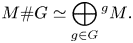
Similarly, we have $M'\#G\simeq \bigoplus _{g\in G} {^g{M'}}$ . Then the ‘only if’ part of (2) follows from the Krull-Schmidt theorem.
For an $A$ -module $M$
 , we have a $G$
 -graded algebra

whose product is given by
for $f\colon M\rightarrow {^gM}$ and $f'\colon M\rightarrow {^hM}$
 . Here, we use the fact that $^h{(^gM)}={^{gh}M}$
 , and observe that $ff'\colon M\rightarrow {^{gh}M}$
 is well defined.
The following isomorphism is well known; see [Reference Reiten and Riedtmann26, Section 3] or [Reference Chen3, Proposition 2.4].
Lemma 7.2 Keep the notation as above. Then there is an isomorphism of algebras
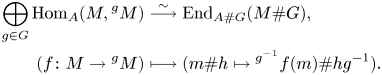
Here, ${^{g^{-1}}f(m)}$ means the element in $M$
 that corresponds to $f(m)\in {^gM}$
 .
.
Proof. We observe that $M\# g^{-1}$ is naturally identified with ${^gM}$
 as a left $A$
 -module. Then the above isomorphism follows from (7.1) and the Hom-tensor adjunction.
Denote by $D={\rm Hom}_{\mathbb {K}}(-,\, \mathbb {K})$ the duality of vector spaces, and by ${\rm Tr}_A(-)$
 the transpose of left or right $A$
 -modules. Recall that the Auslander–Reiten translations are given by $\tau _A=D{\rm Tr}_A$
 and $\tau _A^{-}={\rm Tr}_AD$
 ; see [Reference Auslander, Reiten and Smalø1, IV].
The following general facts seem to be well known; compare [Reference Reiten and Riedtmann26, Lemma 4.2].
Lemma 7.3 Let $M$ and $N$
 be a left $A$
 -module and a right $A$
 -module, respectively.
(1) There are isomorphisms of right $A\# G$
-modules: $DM\#G \simeq D(M\# G)$ and ${\rm Tr}_A(M)\#G\simeq {\rm Tr}(M\#G)$.(2) There are isomorphisms of left $A\#G$
-modules: $DN\#G\simeq D(N\#G)$ and ${\rm Tr}_A(N)\#G\simeq {\rm Tr}(N\#G)$.(3) There are isomorphisms of left $A\#G$
-modules $\tau _A(M)\#G\simeq \tau (M\#G)$ and $\tau ^{-}_A(M)\#G\simeq \tau ^{-}(M\# G)$.


Here, ${\rm Tr}$ and $\tau$
 denote the transpose and Auslander–Reiten translation of $A\# G$
 -modules, respectively.
Proof. We only prove (1), because the proof of (2) is similar, and that (3) follows immediately from (1) and (2).
The first isomorphism is given as follows
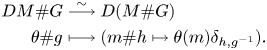
Here, $\delta$ is the Kronecker symbol. For the second one, we first observe a natural isomorphism
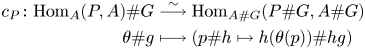
of right $A\#G$ -modules. Take a minimal projective presentation $P_1\rightarrow P_0\rightarrow M\rightarrow 0$
 . Recall that the transpose ${\rm Tr}_A(M)$
 is defined by the following exact sequence

As ${\rm rad}(A)\#G\subseteq {\rm rad}(A\#G)$ , we infer that

is a minimal projective presentation of $M\#G$ . Then the lower exact row of the following commutative diagram follows from the definition of ${\rm Tr}(M\#G)$
 . The upper exact row is obtained by applying $-\#G$
 to (7.3).
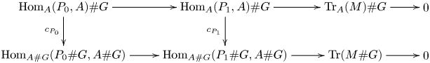
Then the required isomorphism follows immediately.
Recall that a finite dimensional algebra $B$ is local provided that $B/{{\rm rad}(B)}$
 is a division algebra. Following [Reference Auslander, Reiten and Smalø1, p. 65], we say that $B$
 is elementary if $B/{{\rm rad}(B)}$
 is isomorphic to a product of $\mathbb {K}$
 . We observe that a finite dimensional algebra $B$
 is local and elementary if and only if $B/{{\rm rad}(B)}$
 is isomorphic to $\mathbb {K}$
 .
.
Recall from [Reference Nastasescu and Van Oystaeyen25, Section 1.4] that a $G$ -graded algebra $\Gamma =\bigoplus _{g\in G}\Gamma _g$
 is a crossed product if each homogeneous component $\Gamma _g$
 contains an invertible element. Such a crossed product $\Gamma$
 is often denoted by $B\ast G$
 with $B=\Gamma _{(1_G)}$
 .
.
Lemma 7.4 Assume that $\mathbb {K}$ is perfect with ${\rm char}(\mathbb {K})=p>0$
 and that $G$
 is a finite $p$
 -group. Let $B$
 be a finite dimensional algebra which is local and elementary. Then any crossed product $B\ast G$
 , as an ungraded algebra, is local and elementary.
Proof. Take a normal subgroup $N$ of $G$
 such that $G/N$
 is cyclic of order $p$
 . Then $B\ast G=\bigoplus _{g\in G} B_g$
 is naturally $G/N$
 -graded
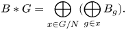
Under this new grading, it is also a cross product. In other words, we have
By induction, it suffices to prove the statement for the case where $G$ is cyclic of order $p$
 .
.
Assume now that $G$ is cyclic of order $p$
 . We will prove that $B\ast G$
 is local and elementary. We will first deal with a special case.
We claim that any crossed product $\mathbb {K}\ast G$ is always local and elementary. Take a generator $g$
 of $G$
 and an invertible element $u_g$
 in $(\mathbb {K}\ast G)_g$
 . We have $(u_g)^p=\mu \in \mathbb {K}$
 for some nonzero $\mu \in \mathbb {K}$
 . Since $\mathbb {K}$
 is perfect, there is some nonzero $\lambda \in \mathbb {K}$
 satisfying $\lambda ^p=\mu$
 . Now the algebra homomorphism
sending $t$ to $\lambda ^{-1}u_g-1$
 , is an isomorphism, proving the claim.
For the general case, we observe that each homogeneous component $B_h$ of $B\ast G$
 is a free $B$
 -module on each side. We observe that $\bigoplus _{h\in G} {\rm rad}(B_h)$
 is a two-sided nilpotent ideal of $B\ast G$
 . Therefore, we have
Recall that $\mathbb {K}\simeq B/{{\rm rad}(B)}$ . Combining the following obvious isomorphism
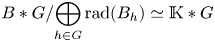
and the above claim, we infer that $B\ast G$ is local and elementary.
Lemma 7.5 Let ${\rm char}(\mathbb {K})=p>0$ and $G$
 be a $p$
 -group. Then the following statements hold.
(1) Assume that $\mathbb {K}$
is perfect. Then any crossed product $\mathbb {K}\ast G$ is local and elementary.(2) Assume that $G$
is cyclic. Then any crossed product $\mathbb {K}\ast G$ is local.


Proof. Since (1) is a special case of lemma 7.4, we only prove (2). Assume that $|G|=q$ for some $p$
 -power $q$
 . Take a generator $g$
 of $G$
 and an invertible element $u_g$
 in $(\mathbb {K}\ast G)_g$
 . We have $(u_g)^q=\mu \in \mathbb {K}$
 for some nonzero $\mu \in \mathbb {K}$
 . We observe a $\mathbb {K}$
 -algebra isomorphism

Then the required statement follows from a standard fact: the algebra $\mathbb {K}[t]/(t^q-\mu )$ is always local.
Let us come back to the situation that a finite group $G$ acts on a finite dimensional algebra $A$
 .
.
Proposition 7.6 Let ${\rm char}(\mathbb {K})=p>0$ and $G$
 be a finite $p$
 -group. Assume that $M$
 is a left $A$
 -module such that ${\rm End}_A(M)$
 is local and elementary. Then the following two statements hold.
(1) Assume that $\mathbb {K}$
is perfect. Then ${\rm End}_{A\#G}(M\#G)$ is local and elementary.(2) Assume that $G$
is cyclic. Then ${\rm End}_{A\#G}(M\#G)$ is local.


In both cases, the $A\#G$ -module $M\#G$
 is indecomposable.
Proof. Denote the $G$ -graded algebra in (7.2) by $\Gamma$
 . By lemma 7.2, it suffices to prove that $\Gamma$
 is local and elementary under the assumption in (1), and local under the assumption in (2), respectively.
Consider the following $G$ -graded subspace of $\Gamma$
Since all the $A$ -modules ${^gM}$
 are indecomposable, it follows that $I$
 is a $G$
 -graded two-sided ideal of $\Gamma$
 . Moreover, it is well known to be nilpotent; for example, see [Reference Auslander, Reiten and Smalø1, VI, Corollary 1.3]. Consequently, we have $I\subseteq {\rm rad}(\Gamma )$
 .
.
Consider the stabilizer $G_M=\{g\in G\; |\; M\simeq {^gM}\}$ of $M$
 . Recall that $\mathbb {K}\simeq {{\rm End}_A(M)}/{{\rm rad}({\rm End}_A(M))}$
 , since ${\rm End}_A(M)$
 is local and elementary. We infer that $\Gamma /I$
 is isomorphic to a crossed product $\mathbb {K}\ast G_M$
 .
.
By the inclusion $I\subseteq {\rm rad}(\Gamma )$ , we have

As $G_M$ is a $p$
 -group, we can apply lemma 7.5 to $\mathbb {K}\ast G_M$
 . Then the required statements follow immediately.
Remark 7.7 Assume that $\mathbb {K}$ is algebraically closed in proposition 7.6. Then for each indecomposable $A$
 -module $M$
 , ${\rm End}_A(M)$
 is local and automatically elementary. It follows that the $A\#G$
 -module $M\#G$
 is indecomposable. In other words, the induction functor

preserves indecomposable modules.
7.2. The folding projection and categorification
In this final subsection, we will always work in the following setup.
Setup ($\clubsuit$ ). Let $\mathbb {K}$
 be a field with ${\rm char}(\mathbb {K})=p>0$
 , and let $G=\langle \sigma \; |\; \sigma ^{p^a}=1_G\rangle$
 be a cyclic group of order $p^a$
 for some $a\geq 1$
 . Let $\Delta$
 be a finite acyclic quiver with $\Delta _0=\{1,\, 2,\, \cdots,\, n\}$
 . Assume that $G$
 acts on $\Delta$
 by quiver automorphisms such that for each arrow $\alpha \in \Delta _1$
 , we have $G_{\alpha }=G_{s(\alpha )}\cap G_{t(\alpha )}$
 .
.
Denote by $\mathbb {Z}\Delta _0=\bigoplus _{i=1}^n \mathbb {Z}\epsilon _i$ the root lattice of $\Delta$
 . It is endowed with a symmetric bilinear form given by $(\epsilon _i,\, \epsilon _i)=2$
 and
and

for $i\neq j$ . Denote by $\Phi ^+(\Delta )$
 the set of positive roots [Reference Kac19].
Denote by $\Delta _0/G$ the orbit set of vertices. The elements in $\Delta _0/G$
 are denoted in the bold form. The canonical projection $\pi \colon \Delta _0\rightarrow \Delta _0/G$
 sends $i$
 to $\pi (i)=Gi=\boldsymbol {i}$
 .
.
Associated to the $G$ -action on $\Delta$
 , we have defined a Cartan triple $(C,\, D,\, \Omega )$
 in §§ 6.2. The rows and columns of $C$
 and $D$
 are indexed by $\Delta _0/G$
 . The entries $c_{\boldsymbol {i}}$
 of $D$
 are determined by
for some $0\leq a_{\boldsymbol {i}}\leq a$ . The corresponding root lattice $\mathbb {Z}(\Delta _0/G)=\bigoplus _{{\boldsymbol {i}}\in \Delta _0/G}\mathbb {Z}E_{\boldsymbol {i}}$
 is endowed with a symmetric bilinear form given by $(E_{\boldsymbol {i}},\, E_{\boldsymbol {i}})=2c_{\boldsymbol {i}}$
 and
and

for $\boldsymbol {i}\neq \boldsymbol {j}$ . Denote by $\Phi ^+(C)$
 the set of positive roots.
There is a canonical projection between the root lattices
given by $\boldsymbol {f}(\epsilon _{i})=E_{\pi (i)}$ , and called the folding projection; see [Reference Springer28, Section 10.3]. It does not preserve the bilinear forms. However, it sends positive roots to positive roots. Moreover, by adapting the proof of [Reference Kac19, Lemma 5.3], [Reference Hubery17, Proposition 15] proves that $\boldsymbol {f}$
 restricts to a surjective map
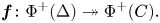
We observe that the folding projection induces an isomorphism between the quotient group of $G$ -coinvariants in $\mathbb {Z}\Delta _0$
 and $\mathbb {Z}(\Delta _0/G)$
 .
.
We mention that there is a folding inclusion from the dual root lattice of $C$ into $\mathbb {Z}\Delta _0$
 , which identifies the dual root lattice with the subgroup of $G$
 -invariants in $\mathbb {Z}\Delta _0$
 ; see [Reference Hubery17, Section 2]. Working with species over a finite field, one observes that the extension-of-scalars functor along a suitable field extension yields a categorification of the folding inclusion; see [Reference Hubery17, the proof of Theorem 24] and [Reference Deng and Du6, Section 9].
Recall that $\mathcal {P}_\Delta$ is the path category of $\Delta$
 . Then the $G$
 -action on $\Delta$
 induces a $G$
 -action on $\mathcal {P}_\Delta$
 . We have the corresponding skew group category $\mathcal {P}_\Delta \rtimes G$
 .
.
We identify the path algebra $\mathbb {K}\Delta$ with the category algebra $\mathbb {K}\mathcal {P}_\Delta$
 . By proposition 2.1, we have the following natural isomorphism of algebras

for any path $q$ in $\Delta$
 and $g\in G$
 .
.
Set $\mathcal {C}=\mathcal {C}(C,\, D,\, \Omega )$ to be the EI category associated to $(C,\, D,\,\Omega )$
 ; see definition 6.1. For each $\boldsymbol {i}\in {\rm Obj}(\mathcal {C})=\Delta _0/G$
 , we have
which is a cyclic group of order $c_{{\boldsymbol {i}}}=p^{a_{{\boldsymbol {i}}}}$ .
.
By theorem 6.6, we identify $\mathcal {C}$ with $\mathcal {C}(\overline {\Delta },\, \overline {U}_{\rm tr})$
 . Fix the choices (5.1) for the $G$
 -action on $\mathcal {P}_\Delta$
 . Then we obtain an equivalence of categories
which satisfies $\iota (\boldsymbol {i})=\iota _0(\boldsymbol {i})$ . The functor $\iota$
 induces the following isomorphism of groups

Recall from definition 6.2 the algebra $H=H(C,\, D,\, \Omega )$ . Each $\boldsymbol {i}$
 corresponds to an idempotent $e_{\boldsymbol {i}}$
 of $H$
 . Moreover, we have

By proposition 6.4, there is an isomorphism of algebras
which identifies $e_{\boldsymbol {i}}He_{\boldsymbol {i}}$ with $\mathbb {K}{\rm Aut}_\mathcal {C}(\boldsymbol {i})$
 . Indeed, we have $\theta (e_{\boldsymbol {i}})={\rm Id}_{\boldsymbol {i}}$
 and $\theta (\varepsilon _{\boldsymbol {i}})=\eta _{\boldsymbol {i}}-{\rm Id}_{\boldsymbol {i}}$
 ; compare remark 6.5.
We now combine (7.4), (7.5) and (7.7) into the following sequence of equivalences.
Here, the two can's mean the canonical equivalence in (2.2), and the upper star functors are given by restriction of scalars. For example, $\iota ^*$ sends a functor $X$
 on $\mathcal {P}\rtimes G$
 to the composite functor $X\circ \iota$
 . We compose the sequence into an equivalence

The following terminology is introduced in [Reference Geiss, Leclerc and Schröer11, Definition 1.1 and Section 11]. A left $H$ -module $Y$
 is locally free, provided that each $e_{\boldsymbol {i}}Y$
 , as an $e_{\boldsymbol {i}}He_{\boldsymbol {i}}$
 -module, is free. For such a module, its rank vector is defined as follows
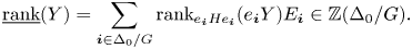
A left $H$ -module $Y$
 is called $\tau$
 -locally free, provided that for any $k\in \mathbb {Z}$
 , $\tau _H^{k}(Y)$
 is locally free. Slightly different from [Reference Geiss, Leclerc and Schröer11], we do not require $\tau$
 -locally free $H$
 -modules to be indecomposable.
Theorem 7.8 Keep the assumptions in Setup ($\clubsuit$ ). Let $M$
 be a left $\mathbb {K}\Delta$
 -module. Then $\Psi (M\#G)$
 is a $\tau$
 -locally free $H$
 -module satisfying

Assume further that ${\rm End}_{\mathbb {K}\Delta }(M)$ is local and elementary. Then ${\rm End}_H(\Psi (M\#G))$
 is local. If moreover $\mathbb {K}$
 is perfect, then ${\rm End}_H(\Psi (M\#G))$
 is local and elementary.
Denote by $H\mbox {-mod}^{\tau \mbox {-lf}}$ the full subcategory of $H\mbox {-mod}$
 consisting of $\tau$
 -locally free modules. The identity (7.8) might be visualized as a commutative diagram.
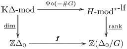
The diagram indicates that the composite functor $\Psi \circ (-\#G)$ categorifies the folding projection $\boldsymbol {f}$
 between the root lattices.
It is natural to categorify the folding projection $\boldsymbol {f}\colon \Phi ^+(\Delta )\rightarrow \Phi ^+(C)$ between the positive roots using the same functor between indecomposable modules. However, we have to restrict to the Dynkin cases; see proposition 7.9.
Proof. Step 1. We first show that the $H$ -module $\Psi (M\#G)$
 is locally free and satisfies the required identity for the rank vector.
Recall that the isomorphism $\theta$ identifies $e_{\boldsymbol {i}}He_{\boldsymbol {i}}$
 with $\mathbb {K}{\rm Aut}_\mathcal {C}(\boldsymbol {i})$
 . Therefore, it suffices to claim that for each $\boldsymbol {i}\in {\rm Obj}(\mathcal {C})=\Delta _0/G$
 ,
,
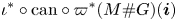
is a free module over $\mathbb {K}{\rm Aut}_\mathcal {C}(\boldsymbol {i})$ with rank
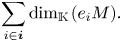
Here, we view $\iota ^*\circ {\rm can}\circ \varpi ^*(M\# G)$ as a functor over $\mathcal {C}$
 .
.
For the claim, we observe the following identity.
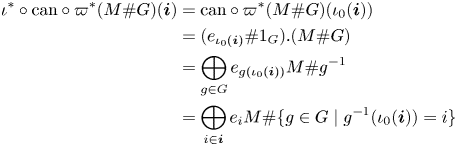
Here, for the second equality we recall that the trivial path $e_{\iota _0(\boldsymbol {i})}$ is the identity endomorphism of $\iota _0(\boldsymbol {i})$
 in $\mathcal {P}_\Delta$
 , and for the third one, we use the fact that $g(e_{\iota _0(\boldsymbol {i})})=e_{g(\iota _0(\boldsymbol {i}))}$
 .
.
By (7.6), we identify $\mathbb {K}{\rm Aut}_\mathcal {C}(\boldsymbol {i})$ with $\mathbb {K}G_{\iota _0(\boldsymbol {i})}$
 . As $G$
 is abelian, we have $G_{\iota _0(\boldsymbol {i})}=G_i$
 for each $i\in \boldsymbol {i}$
 . Then we observe that the left $\mathbb {K}G_{\iota _0(\boldsymbol {i})}$
 -action on the above direct summand
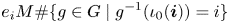
is really only on the right side, that is, on the set $\{g\in G\; |\; g^{-1}(\iota _0(\boldsymbol {i}))=i\}$ via the multiplication in $G$
 . The latter $G_{\iota _0(\boldsymbol {i})}$
 -action is free and transitive. Therefore, the $G_{\iota _0(\boldsymbol {i})}$
 -action on the above direct summand is free of rank ${\rm dim}_\mathbb {K}(e_iM)$
 . This observation implies the claim.
Step 2. Since $\Psi$ is an equivalence, it commutes with Auslander–Reiten translations. Then we have isomorphisms

where the isomorphism on the right side follows from lemma 7.3. Here, the unadorned $\tau$ means the Auslander–Reiten translation of $\mathbb {K}\Delta \# G$
 -modules. By Step 1, we infer that each $H$
 -module $\tau _H^k\Psi (M\#G)$
 is locally free, that is, $\Psi (M\#G)$
 is $\tau$
 -locally free.
The equivalence $\Psi$ induces an isomorphism of algebras

Then the last statement follows from proposition 7.6.
Denote by $\mathbb {K}\Delta \mbox {-ind}$ a complete set of representatives of indecomposable $\mathbb {K}\Delta$
 -modules. Similarly, $H\mbox {-ind}^{\tau \mbox {-lf}}$
 is a complete set of representatives of indecomposable $\tau$
 -locally free $H$
 -modules. As $G$
 acts on $\mathbb {K}\Delta \mbox {-ind}$
 by twisting endofunctors, we have the orbit set $\mathbb {K}\Delta \mbox {-ind}/G$
 .
.
Proposition 7.9 Keep the assumptions in Setup ($\clubsuit$ ). We assume further that $\Delta$
 is of Dynkin type. Then the following commutative diagram is well defined
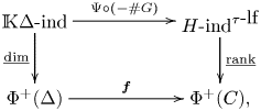
whose vertical arrows are bijections. In particular, the map $\Psi \circ (-\#G)$ induces a bijection
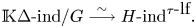
Proof. We observe that $C$ is also of Dynkin type; compare [Reference Chen and Wang4, Proposition 6.5]. The map $\underline {\rm dim}$
 is bijective by the well-known Gabriel's theorem; see [Reference Gabriel9, 1.2 Satz] and [Reference Auslander, Reiten and Smalø1, VIII.5]. By [Reference Geiss, Leclerc and Schröer11, Theorem 1.3], the map $\underline {\rm rank}$
 is bijective.
It is well known that each indecomposable $\mathbb {K}\Delta$ -module $M$
 satisfies ${\rm End}_{\mathbb {K}\Delta }(M)\simeq \mathbb {K}$
 ; for example, see [Reference Auslander, Reiten and Smalø1, VIII, Lemma 6.1]. We infer from theorem 7.8 that the $H$
 -module $\Psi (M\#G)$
 is indecomposable. Then the above commutative diagram is well defined. Since $\boldsymbol {f}\colon \Phi ^+(\Delta )\rightarrow \Phi ^+(C)$
 is surjective, we infer that the map
is surjective. In view of lemma 7.1, we have the induced bijection.
Remark 7.10
(1) We mention that any non-symmetric Cartan matrix $C$
of Dynkin type does appear in the situation of proposition 7.9; see [Reference Lusztig23, 14.1.6] or [Reference Chen and Wang4, p.81, Table 1]. The representation theory related to the folding inclusion in the Dynkin cases is studied in [Reference Tanisaki30].(2) Since [Reference Geiss, Leclerc and Schröer11, Theorem 1.3] works currently only for Dynkin cases, we do not know how to extend proposition 7.9 to non-Dynkin quivers.

In view of [Reference Kac18] and [Reference Deng and Xiao7, 3.3 Theorem], the following open question in [Reference Geiss, Leclerc and Schröer12, Conjecture 5.3], analogous to Kac's theorem, is very natural: does the set of rank vectors of indecomposable $\tau$ -locally free $H$
 -modules coincide with $\Phi ^+(C)$
 ? We refer to [Reference Geiss, Leclerc and Schröer13] for related consideration on rigid locally free $H$
 -modules, and [Reference Huang, Lin and Su16] for an affirmative answer to the question in type $\tilde {C}_n$
 .
.
Assume that $\mathbb {K}$ is algebraically closed. By [Reference Kac18, Theorem 2], for any $\alpha \in \Phi ^+(\Delta )$
 , there is an indecomposable $\mathbb {K}\Delta$
 -module $M$
 with $\underline {\rm dim}(M)=\alpha$
 . Combining the surjectivity of $\boldsymbol {f}\colon \Phi ^+(\Delta )\rightarrow \Phi ^+(C)$
 and theorem 7.8, we infer the following fact: for each $\beta \in \Phi ^+(C)$
 , there is an indecomposable $\tau$
 -locally free $H$
 -module $X$
 with $\underline {\rm rank}(X)=\beta$
 . This fact supports an affirmative answer to the above open question.
We illustrate proposition 7.9 with an explicit example.
Example 7.11 Let $\mathbb {K}$ be a field of characteristic two, and let $\Delta$
 be the following quiver of type $A_3$
 .
.
The Auslander–Reiten quiver $\Gamma _{\mathbb {K}\Delta }$ is as follows.
Here, the dotted arrows denote the Auslander–Reiten translation. We visualize each module using its radical layers, and represent composition factors by their corresponding vertices.
Let $G=\{1_G,\, \sigma \}$ be a cyclic group of order two, and let $\sigma$
 act on $\Delta$
 by interchanging $\alpha$
 and $\alpha '$
 . The associated Cartan triple $(C,\, D,\, \Omega )$
 is of type $B_2$
 and given as follows:

The algebra $H=H(C,\, D,\, \Omega )$ is given by the following quiver
subject to relations $\varepsilon _1^2=0=\varepsilon _2$ . In practice, one simply deletes the loop $\varepsilon _2$
 .
.
The Auslander–Reiten quiver $\Gamma _H$ is as follows; see [Reference Geiss, Leclerc and Schröer11, Subsection 13.6].
Here, the leftmost and rightmost arrows in the bottom are identified. We have framed all the indecomposable $\tau$ -locally free $H$
 -modules. The central three-dimensional $H$
 -module is locally free, but not $\tau$
 -locally free.
We apply proposition 7.9 to obtain the bijection

The twisting endofunctor on $\mathbb {K}\Delta \mbox {- mod}$ with respect to $\sigma$
 turns $\Gamma _{\mathbb {K}\Delta }$
 upside down. By comparing $\Gamma _{\mathbb {K}\Delta }$
 and $\Gamma _H$
 , we observe that $\Theta$
 preserves the frames of the modules, that is, each indecomposable $\mathbb {K}\Delta$
 -module $M$
 and $\Theta (M)$
 have the same kind of frames.
By lemma 7.3, the bijection $\Theta$ is compatible with Auslander–Reiten translations. The following observation might be compared with [Reference Reiten and Riedtmann26, Theorem 3.8]: by applying $\Theta$
 to the square in $\Gamma _{\mathbb {K}\Delta }$
 , we infer that, in general, $\Theta$
 does not preserve Auslander–Reiten sequences.
Acknowledgements
We thank the referee for helpful comments. This paper is partly written when Wang visited University of Stuttgart in 2019; she is grateful to Steffen Koenig for inspiring comments and his hospitality. Chen thanks Jan Schröer for a helpful email concerning remark 7.10(2). We thank Bernhard Keller for enlightening discussions. This work is supported by National Natural Science Foundation of China (No.s 12325101, 12131015 and 12161141001).


