


1. Introduction
Fronts, or regions with large horizontal density gradients, are common features of the ocean surface mixed layer. The strength of a front is measured by the horizontal analogue to the buoyancy frequency,  $M^2 \equiv |\nabla _h \bar {b}|$, where $\bar {b} \equiv -g\bar {\rho }/\rho _0$ is the background buoyancy field, $\nabla_h$ is the lateral gradient operator, $g$ is the acceleration due to gravity and $\rho _0$ is a reference density. In frontal regions stable to both gravitational and inertial instability, symmetric instability (SI) can still grow if the magnitude of the isopycnal slope, $M^2/N^2$ (for $N^2 \equiv \partial _z \bar {b}$), exceeds a certain threshold. Specifically, a front is unstable to SI when the Ertel potential vorticity (PV)
 \begin{equation} q \equiv (\,f \hat{\boldsymbol{z}} + \boldsymbol{\nabla} \times \boldsymbol{u}) \boldsymbol{\cdot} \boldsymbol{\nabla} b, \end{equation}
(defined with the full velocity,  $\boldsymbol {u}$, and with $\hat {\boldsymbol {z}}$ the vertical unit vector) is of the opposite sign to the Coriolis parameter, $f$ (Hoskins Reference Hoskins1974). The growing SI modes resemble slanted convection cells and are independent of the along-front direction (i.e. perpendicular to the horizontal buoyancy gradient) (Stone Reference Stone1966).
In Part 1 (Wienkers, Thomas & Taylor Reference Wienkers, Thomas and Taylor2021, hereafter referred to as Part 1) we described the dependence of SI growth and saturation on the front strength parameterised by  $\varGamma \equiv M^2/f^2$. There, we considered the linear growth and weakly nonlinear saturation of SI in the idealised problem consisting of a broad frontal zone with a uniform horizontal buoyancy gradient in thermal wind balance and bounded by flat no-stress horizontal surfaces. We found that, depending on $\varGamma$ and $Ri \equiv N^2f^2/M^4$, the front can extract energy primarily from either the kinetic energy of the balanced thermal wind or from the potential energy of the background density profile. Strong fronts are dominated by geostrophic shear production, $\mathcal {P}_g$, and we distinguished this SI as ‘slantwise inertial instability.’ In contrast, fronts with small $\varGamma$ or $Ri \gtrsim 0.5$ see SI energised more by buoyancy production, $\mathcal {B}$, and we called this flavour of SI ‘slantwise convection.’
Subsequent to extracting energy from the balanced thermal wind, we found that SI can induce vertically sheared inertial oscillations with varying amplitude depending on  $\varGamma$. We hypothesised that the fraction of the thermal wind mixed down by SI and the ensuing turbulence can be related to the amplitude of the subsequent inertial oscillations by using the theory of Tandon & Garrett (Reference Tandon and Garrett1994). We computed their parameter $s$,
$s$,
 \begin{equation} \left. s \equiv \frac{f}{M^2} \frac{\partial\bar{v}}{\partial z}\right|_{t=\tau_c}, \end{equation}
(using the horizontally averaged along-front velocity,  $\bar {v}$) to quantify the degree of imbalance after the saturation of SI at $\tau _c$ (cf. figure 8(b) in Part 1). We then concluded that, because a higher fraction of the thermal wind is mixed, stronger fronts will exhibit larger-amplitude inertial oscillations following destabilisation by SI. Finally, we calculated the SI momentum transport time scale, $\tau _{mix}$ (cf. figure 8a in Part 1), needed to homogenise the thermal wind. We found that $\tau _{mix} > f^{-1}$ for $\varGamma < 8$, which suggests that weak fronts should exhibit a slow quasi-balanced evolution to equilibrium. In contrast, strong fronts are expected to rapidly mix the thermal wind and undergo geostrophic adjustment.
This theoretical handling of the SI induced equilibration of balanced fronts has left a number of questions unanswered. Specifically, the nonlinear consequences of these results from Part 1 – of the energy sources and thermal wind mixing rate, which were shown to strongly depend on  $\varGamma$ – are expected to influence the later evolution of the front beyond the initial saturation of SI. We use the framework of Tandon & Garrett (Reference Tandon and Garrett1994) to shed light on the effects of dissipation and a finite mixing time on the adjustment and resulting inertial oscillations. They considered the geostrophic evolution of an instantaneously mixed unstratified front. However, particularly in weak fronts, this $\tau _{mix}$ may be longer than the inertial period, and so the resulting adjustment may instead resemble a turbulent thermal wind balance (Gula, Molemaker & McWilliams Reference Gula, Molemaker and McWilliams2014). In the opposite limit of strong fronts, the excited inertial oscillations can modulate the growth rate of residual SI. This leads to periods of explosive growth and turbulence corresponding with times when the front is weakly stratified (Thomas et al. Reference Thomas, Taylor, D'Asaro, Lee, Klymak and Shcherbina2016).
Other numerical process studies of SI have investigated the nonlinear evolution in varying configurations, but most have focused only on a single value of the non-dimensional horizontal buoyancy gradient (Thomas & Lee Reference Thomas and Lee2005; Taylor & Ferrari Reference Taylor and Ferrari2009, Reference Taylor and Ferrari2010; Thomas & Taylor Reference Thomas and Taylor2010; Stamper & Taylor Reference Stamper and Taylor2016). In this paper, we extend the theory developed in Part 1 which described the effect of varying the front strength on the growth and saturation of SI. We use a set of two-dimensional (2-D) numerical simulations spanning a large range of  $\varGamma$ to understand the extent to which the geostrophic momentum mixing induced by SI and turbulence either directly or indirectly prompts a response similar to that of Tandon & Garrett (Reference Tandon and Garrett1994).
We begin in § 2 by briefly describing the physical problem set-up, which matches that used in Part 1, but here for the special case of a front which is initially vertically unstratified. We detail the numerical model and set of simulations in § 3, and provide an overview of the general evolution of these fronts. In § 4, we show how each front is forced out of thermal wind balance and suggest how the rate of adjustment influences the inertial oscillations considered in § 5. There, we examine the vertical structure and evolution of these inertial oscillations as well as their damping and contribution to the equilibration of the front. Finally, in § 6 we consider the feedbacks of the front generating late-time SI and modulating the turbulence. We further describe how these persistent SI modes can generate frontlets and bore-like gravity currents, and consider how this behaviour scales with front strength.
2. Problem set-up
We consider the same configuration of the Eady model as studied in Part 1 (Eady Reference Eady1949). In this context, the Eady model can be viewed as an idealised mixed layer front where the bottom of the mixed layer is replaced by a flat, rigid boundary. Explicitly, this set-up comprises an incompressible flow in thermal wind balance with a uniform horizontal buoyancy gradient, and bounded between two rigid, stress-free horizontal surfaces.
We choose the dimensionless units of this problem such that the balanced thermal wind shear ( $M^2/f$) and the vertical domain size ( $H$) are both unity. This results in four dimensionless parameters, shown here with the values used to reduce the parameter space
 \begin{equation} \varGamma \equiv \frac{M^2}{f^2}; \quad Re \equiv \frac{H^2 M^2}{f \nu} = 10^5; \quad Ri_0 \equiv \frac{N_0^2 f^2}{M^4} = 0; \quad Pr \equiv \frac{\nu}{\kappa} = 1, \end{equation}
where the subscript  $0$ indicates the initial value of an evolving quantity. Here, $\nu$ is the kinematic viscosity and $\kappa$ is the diffusivity of buoyancy, but we take $Pr = 1$ to match the theory presented in Part 1. We further reduce the parameter space by considering initial conditions with no stratification ( $N_0^2 = 0$). This choice was made because unstratified fronts were found to have the most varied behaviour across $\varGamma$ from the theory in Part 1. Finally, it should be noted that the Rossby number is not an independent parameter but can be related to the Richardson number for motions with a given aspect ratio (Stone Reference Stone1966).
We solve the Boussinesq equations on an  $f$-plane and neglect the non-traditional Coriolis terms. These non-dimensionalised governing equations are
 $$\begin{gather} \frac{\textrm{D} \boldsymbol{u}^*}{\textrm{D} t^*} ={-}\boldsymbol{\nabla}^*\varPi^* - \frac{1}{\varGamma} \hat{\boldsymbol{z}}\times \boldsymbol{u}^* + \frac{1}{Re} \nabla^{*2}\boldsymbol{u}^* + b^* \hat{\boldsymbol{z}} \end{gather}$$
 $$\begin{gather}\frac{\textrm{D} b^*}{\textrm{D} t^*} = \frac{1}{Re} \nabla^{*2} b^* \end{gather}$$
 $$\begin{gather}0 = \boldsymbol{\nabla}^*\boldsymbol{\cdot} \boldsymbol{u}^*, \end{gather}$$
where the dimensionless ( $^*$) variables are
 \begin{equation} \boldsymbol{u}^* \equiv \boldsymbol{u}\frac{f}{H M^2}; \quad b^* \equiv b \frac{f^2}{H M^4}; \quad t^* \equiv t \frac{M^2}{f}; \quad \boldsymbol{x}^* \equiv \boldsymbol{x}\frac{1}{H}; \quad \boldsymbol{\nabla}^* \equiv H \boldsymbol{\nabla}. \end{equation}
The dimensionless pressure head acceleration,  $\boldsymbol{\nabla} ^* \varPi ^*$, absorbs the hydrostatic pressure gradient, but otherwise acts only as a Lagrange multiplier to satisfy the incompressibility constraint (2.2c). Because we focus on inertial times after the critical (SI saturation) point, $\tau _c$, we will often use the dimensionless inertial time variable
 \begin{equation} t_f^* \equiv ( t - \tau_c ) f = ( t^* - \tau_c^* ) \varGamma^{{-}1}, \end{equation}
with corresponding frequency,  $\omega _f^* \equiv \omega /f$, which is also non-dimensionalised by the inertial frequency, $f$.
$f$.
The initial condition is a balanced thermal wind ( $v_g$) in the invariant along-front ( $\hat {\boldsymbol {y}}$) direction, which balances the baroclinic torque of the uniform buoyancy gradient in the across-front ( $\hat {\boldsymbol {x}}$) direction
 \begin{equation} \left. \begin{array}{c@{}} v^*_0 = z^* - 1/2 \\ b^*_0 = \varGamma^{{-}1} x^* \end{array}\right\}. \end{equation}
Finally, the boundary conditions at  $z^* = 0$ and $1$ are taken to be insulating and stress free. In what follows we will omit the appended asterisks for notational simplicity. All variables are dimensionless unless the units are explicitly stated (as in some figures).
3. Numerical simulations
We used the non-hydrostatic hydrodynamics code, diablo, to integrate the fully nonlinear Boussinesq equations (2.2) (Taylor Reference Taylor2008). diablo uses second-order finite differences in the vertical and a collocated pseudo-spectral method in the horizontal periodic directions, along with a third-order accurate implicit-explicit time-stepping algorithm using Crank–Nicolson and Runge–Kutta with an adaptive step size.
These simulations are run in a 2-D ( $x$–
$x$– $z$) domain oriented across the front, while still retaining all three components of the velocity vector. This choice allows us to focus on the evolution of the symmetric (i.e. $y$-invariant) modes. It should be noted that the thermal wind shear in this particular setup would be susceptible to Kelvin Helmholtz instability (KHI) along the front in a 3-D simulation, but this is not considered for the purpose of this study. Still, we present the results of short 3-D large-eddy simulations in Appendix A to confirm that the following results for SI are robust in three dimensions.
Each of the 2-D simulations with  $\varGamma = \{1, 10, 100\}$ were run until time $100\varGamma$, except for the $\varGamma = 100$ case which was only run until $t = 40\varGamma$. The computational cost scales as $\varGamma ^2$ due to the requirement for a shorter time step and a larger domain. But the large aspect ratio of the domain (having across-front length, $L_x \sim \varGamma$) means that the additional computation is not conducive to parallelisation. Each simulation was initialised as an unstratified balanced front (2.5) with $Ri_0=0$. White noise was added to the velocity with a (dimensionless) amplitude of $10^{-4}$. We do not vary the Reynolds number across experiments, which is $Re = 10^5$. Many of the other parameters and details of the runs are summarised in table 1.
Table 1. Summary of the details of each numerical simulation along with a few specific values from the theory presented in Part 1. All quantities are dimensionless. The physical dimensions of the domain,  $(L_x,L_y,1)$, along with the corresponding number of Fourier modes or grid points, $(N_x, N_y, N_z)$. The wavelength, $\lambda _{SI}$, and growth rate, $\sigma _{SI}$, of the fastest growing linear SI mode corresponding to (2.5). The SI thermal wind mixing fraction, $(1-s)$, and dimensionless mixing time scale, $\tau _{mix}$, predicted in Part 1, and which imply the inertial oscillation amplitude. The critical time, $\tau _c$, when SI breaks down via KHI in each simulation.

The nonlinear simulations help to paint a picture of this frontal dynamics – from SI and KHI-generated turbulence, through adjustment and inertial oscillations, as well as late-time SI and further shear instabilities taking the front to equilibrium. While the specific details vary depending on  $\varGamma$, three distinct phases are seen in each simulation:
(i) Linear SI energises a broad wavenumber spectrum (apparent before the critical time of turbulent transition, $\tau _c$, in figure 2) due to the weak scale and vertical mode ($n$) dependence of SI growing from the initial white noise perturbations. This means that a range of SI scales are represented and combine to contribute to the SI transport and dynamics. Nonetheless, the predictions from linear theory (based on the fastest growing mode) still appear to be remarkably consistent. For example, symbols in figure 3(b) from Part 1 show the growth rate and turbulent kinetic energy (TKE) budget terms extracted from the simulations in the linear SI phase.
(ii) As the SI modes reach a critical amplitude,
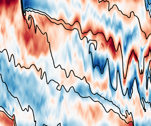
$U_{c}$, secondary shear instability converts much of this coherent energy into small-scale turbulence (left column of figure 1). The SI and turbulence remove energy from the background geostrophic shear flow and induce vertically sheared inertial oscillations.(iii) In the late stages of each simulation, larger-scale SI modes grow and periodically exhibit KHI at times when the vertically sheared inertial oscillation de-stratifies the front (e.g. right column of figure 1). These late-time SI modes inject positive PV from the boundaries into the domain interior which permits the ageostrophic circulation to re-stratify the front, eventually to
$Ri = 1$. Once the mean $fq \gtrsim 0$, SI is neutralised but the inertial oscillations may still remain.


Figure 1. Slices across each front show the along-front vorticity,  $\omega _y \equiv (\partial _z u - \partial _x w)$, along with buoyancy contours (black lines), for $\varGamma = 1$ (top), $10$ (centre), and $100$ (bottom). Two time snapshots are shown: at $t = \tau _c$ (left) when secondary KHI first begins to break the coherent energy of the SI modes into small-scale turbulence, and at a later time $t_2$ (right) when SI again develops and subsequently rolls up into Kelvin–Helmholtz instability while the vertically sheared inertial oscillation de-stratifies the front. (Here, $t_2$ corresponds to times when $t_f/(2{\rm \pi} ) = 10$, $5$ and $2$, respectively for Γ = 1, $10$, and $100$.) Note that the vorticity is normalised by $M$, which keeps the amplitude similar across the range of $\varGamma$. The vorticity normalised by $f$ can be obtained by multiplying the values shown here by $\varGamma ^{-1/2}$. Note that only a subset of the horizontal domain is shown for both $\varGamma = 10$ and $100$.

Figure 2. Time series of the across-front wavenumber,  $k_x$ (right), extracted from the 2-D $\varGamma = 1$ simulation are compared alongside the linear growth rates (left) for each of the vertical modes $n = \{1, 2, 4, 8, 16, 32\}$. Wavenumbers of peak linear growth are indicated with horizontal white bars and emphasise the weak wavenumber and vertical mode selection during the linear phase. Remnants of late-time SI with larger wavelengths are modulated by the inertial oscillations and is apparent once the front has re-stratified and after $t_f \approx 50$. Subinertial oscillations around $k_x = 8$ are also visible.

Figure 3. The horizontally averaged  $x$- and $y$-momentum budget (4.1) at $z = 3/4$ for $\varGamma = 10$. The red shaded region highlights the period when the dominant balance is described by SI-induced Reynolds stresses (red line) accelerating the mean along-front $y$-momentum (blue line). The linear SI mode transport at saturation is also shown. Following this ageostrophic perturbation, the front begins inertially oscillating. Grey shaded regions indicate periods when the Reynolds stress divergence damps the inertial oscillations (i.e. when $\bar {u}_a > 0$ coincident with $-\partial _z\overline {u'w'} < 0$).
4. Loss of geostrophic balance
The effect of turbulent stresses on the mean circulation is described by the horizontally (x, y) averaged ageostrophic momentum equations,
 $$\begin{gather} \partial_t \bar{u}_a + \partial_z\overline{u'w'} = \varGamma^{{-}1}\bar{v}_a, \end{gather}$$
 $$\begin{gather}\partial_t \bar{v}_a + \partial_z\overline{v'w'} ={-}\varGamma^{{-}1}\bar{u}_a, \end{gather}$$
where the primed variables represent local fluctuations from the horizontally averaged fields denoted by an overbar:  $\xi ' \equiv \xi - \bar {\xi }$. We showed in Part 1 that SI influences the larger-scale, horizontally averaged evolution of the front through these turbulent Reynolds stresses on the left side.
4.1. Exchange of dominant balance
For  $\varGamma \gtrsim 1$ and $Ri \lesssim 0.5$ the linear theory indicates that the mean ageostrophic $y$-momentum is generated before ageostrophic $x$-momentum. As a result, the dominant balance of (4.1) is initially
 \begin{equation} \partial_t\bar{v}_a \approx{-}\partial_z\overline{v'w'}.\end{equation}
We can test this by computing the turbulent momentum budget described by (4.1) on a particular horizontal plane,  $z = 3/4$, away from boundary effects and off of the mid-plane (where $\bar {\boldsymbol {u}}_a \approx 0$). This initial dominant balance (4.2) is responsible for destabilising the front and demonstrates how inertial oscillations are driven during the $\varGamma = 10$ simulation (figure 3). More specifically, the Reynolds stress divergence accelerates the mean ageostrophic $y$-momentum through the first half of the inertial period (highlighted by the red shaded region in panel b). At the same time, the mean across-front $x$-momentum (panel a) is primarily influenced by SI only through the Coriolis term (yellow line) coupling to $\bar {v}_a$, even during the first inertial period.
On the (inertial) time scale,  $\varGamma$ (i.e. when $\bar {v}_a$ is large enough), the dominant balance returns to
 \begin{equation} \partial_t\bar{\boldsymbol{u}}_a \approx{-}\varGamma^{{-}1} \hat{\boldsymbol{z}}\times\bar{\boldsymbol{u}}_a. \end{equation}
However, the ageostrophic perturbations generated by SI mean that  $\bar {\boldsymbol {u}}_a \ne 0$. Thus this balance now describes the undamped inertial oscillations which we will focus on in § 5. These two phases of adjustment are most distinct when SI acts to quickly (on a time scale much faster than $\varGamma$) influence the balanced thermal wind. This will be quantified in § 4.3 below.
4.2. Adjustment energetics
Both potential energy and geostrophic kinetic energy associated with the balanced front can be extracted by SI. The vertically sheared inertial oscillations that develop in response to SI add another component to the system: mean ageostrophic kinetic energy. Here, we investigate the energetics as SI saturates and the front adjusts to the loss of thermal wind balance.
In our dimensionless units, the mean kinetic energy (MKE) of the geostrophic flow is  $\overline {E_K}_{,g} = 1/24$. Although the equilibrated front (also in thermal wind balance) has the same MKE, imperfect mixing of the thermal wind shear by fraction $(1-s)$, taking it to an intermediate state, $\bar {v}_s = s \bar {v}_g$, can temporarily release an amount of kinetic energy equal to
 \begin{align} {\rm \Delta} \overline{E_K} &= \tfrac{1}{2}\int_0^1 (\bar{v}_g^2 - \bar{v}_s^2) \, \mathrm{d}z \nonumber\\ &= \tfrac{1}{24} (1-s^2). \end{align}
Meanwhile, the uniform background buoyancy gradient,  $\partial _x \bar {b}$, represents a reservoir of potential energy. It is useful to define the mean potential energy (MPE) as ${\overline {E_P} \equiv -\langle z(\bar {b}-\bar {b}_f) \rangle }$, where $\langle \cdot \rangle$ indicates a volume average over the entire domain. This MPE is defined relative to the final state, $\bar {b}_f$, with $q=0$ (equivalently $Ri=1$) which is the lowest potential energy before SI shuts down. If we assume a linear mean buoyancy profile, $\bar {b} \propto z$, such that $\partial _z\bar {b}=1$ when $Ri=1$, then the MPE can be approximated as
 \begin{equation} \overline{E_P} \approx \int_0^1 -z^2(\partial_z\bar{b} - 1) \, \mathrm{d}z = \tfrac{1}{3} (1 - Ri). \end{equation}
Thus our choice of  $Ri_0 = 0$ gives the maximum potential energy available to SI through equilibration: ${\rm \Delta} \overline {E_P} = 1/3$ (in geostrophic units). The distance, $\mathcal {L}_d$, that the front will ultimately slump to reach this state of $0$ ‘SI-available’ potential energy is $\mathcal {L}_d = \varGamma$.
Now that we have quantified the size of these energy reservoirs, we gain further insight into the evolution and equilibration of the front by considering the transfers between them. We summarise the energetics of the  $\varGamma =10$ simulation in figure 4, which shows qualitatively similar features to the other fronts even though the relative importance of each term varies. At the start of the simulation, geostrophic shear production, $\mathcal {P}_g$, energises SI by extracting energy from the MKE of the thermal wind and converting it into TKE, ${E_K \equiv \frac {1}{2}\langle u_i' u_i'\rangle }$, which evolves as
 \begin{equation} \frac{\partial E_K}{\partial t} = \underbrace{-\left\langle \overline{v'w'}\frac{\partial\bar{v}_g}{\partial z}\right\rangle }_{\mathcal{P}_g} +\underbrace{-\left\langle \overline{u'w'}\frac{\partial\bar{u}}{\partial z}-\overline{v'w'}\frac{\partial\bar{v}_a}{\partial z}\right\rangle }_{\mathcal{P}_a} + \underbrace{\langle w'b'\rangle }_\mathcal{B} - \underbrace{\frac{1}{Re}\left\langle \frac{\partial u'_i}{\partial x_j}\frac{\partial u'_i}{\partial x_j}\right\rangle }_{\varepsilon_t}.\end{equation}
While some of this energy is immediately dissipated ( $\varepsilon _t$), part of it is subsequently converted (via $\mathcal {P}_a<0$) to ageostrophic MKE, $\overline {E_K}_{,a} \equiv \frac {1}{2} \langle \bar {u}_{i,a} \bar {u}_{i,a} \rangle$, which for this system evolves as
 \begin{equation} \frac{\partial \overline{E_K}_{,a}}{\partial t} = \underbrace{-\frac{1}{Re}(\bar{v}_a|^{z=1}_{z=0})}_{\mathrm{Surface \ stress}} + \underbrace{\left\langle \overline{u'w'}\frac{\partial \bar{u}}{\partial z} + \overline{v'w'}\frac{\partial \bar{v}_a}{\partial z}\right\rangle }_{-\mathcal{P}_a} - \underbrace{\frac{1}{Re}\left\langle \left(\frac{\partial \bar{u}}{\partial z}\right)^2 + \left(\frac{\partial \bar{v}_a}{\partial z}\right)^2 \right\rangle }_{\varepsilon_{m,a}}. \end{equation}
The negative ageostrophic shear production,  $\mathcal {P}_a$, (particularly during the highlighted blue region in figure 4) implies an energy transfer into ageostrophic MKE and reflects the excitation of inertial oscillations.

Figure 4. A summary of the energy transfers (top) and reservoirs (bottom) co-evolving for the  $\varGamma = 10$ front. In this front, SI and turbulence is primarily energised by $\mathcal {P}_g$ which transfers energy from MKE into TKE. At the same time, the ageostrophic shear production ( $\mathcal {P}_a$) is negative in the first half of the inertial period (highlighted by the blue region) suggesting that inertial oscillations are being energised. Because we show just the ageostrophic MKE here, these inertial oscillations which continually exchange MKE and MPE can only be inferred from the MPE. This energy in the mean ageostrophic motions is also converted back into TKE when $\mathcal {P}_a > 0$. This primarily occurs as the vertically sheared inertial oscillation steepens isopycnals (i.e. when $\mathrm {d}/\mathrm {d}t(\overline {E_P})>0$, highlighted in grey).
While it is not shown in the energy transfers of figure 4(a), the inertial oscillations involve continual exchange of ageostrophic MKE and MPE. This exchange occurs via the mean advection of the horizontal buoyancy gradient, which modifies the vertical stratification, and in the process converts energy from the MPE at a rate of
 \begin{equation} \partial_x \bar{b} \langle \bar{u} z \rangle . \end{equation}
Energy in the mean inertial oscillation ultimately can be converted back into TKE via the ageostrophic shear production when  $\mathcal {P}_a > 0$. This occurs here at times when the inertial oscillations steepen isopycnals as in Thomas et al. (Reference Thomas, Taylor, D'Asaro, Lee, Klymak and Shcherbina2016) (and $\mathrm {d}/\mathrm {d}t(\overline {E_P})>0$ as highlighted by the grey regions in figure 4). During these times the ageostrophic MKE decreases as seen in the integrated energy in the bottom panel. The last source of TKE in (4.6) is from buoyancy production, $\mathcal {B}$. However, particularly for this $\varGamma = 10$ front (and stronger fronts) this source of energy does not have a significant influence on the front.
4.3. Rate of adjustment
We will now analyse the time scales involved in the onset of inertial oscillations and find two limiting behaviours depending on the front strength. We can visualise these differences in the speed of adjustment by considering hodographs of this measure of the mean bulk shear
 \begin{equation} \langle |\bar{\boldsymbol{u}}|\rangle = 2 \left[ \int_{1/2}^{1} \bar{\boldsymbol{u}}(z) \, \mathrm{d}z-\int_0^{1/2} \bar{\boldsymbol{u}}(z) \, \mathrm{d}z \right]. \end{equation}
Perfect inertial oscillations in this  $\langle |\bar {u}|\rangle$– $\langle |\bar {v}|\rangle$ phase space therefore trace circles. This metric is also less contaminated by the boundary layers as would be if simply computing $\langle \partial _z \bar {\boldsymbol {u}}\rangle$. We show these hodographs of $\langle |\bar {\boldsymbol {u}}|\rangle$ in figure 5(a) for each simulation with increasing $\varGamma$ from left to right, and can see how this metric (4.9) corresponds to the full structure of a typical inertial period as shown in figure 5(b). The axes are in units of the thermal wind so that the initial balanced state is $\langle |\bar {\boldsymbol {u}}|\rangle = (0,1)$. Starting at $t = 0$ (designated with a black dot) each front departs from the geostrophic balance and begins tracing inertial trajectories. Perhaps the most obvious difference is in the radius of these inertial circles. A front that is instantaneously vertically mixed by a fraction $(1-s)$ will trace circles with radius $(1-s)$. We find the amplitude of these oscillations to be in general agreement with the linear SI transport theory to compute $(1-s)$ as presented in Part 1, and reproduced in table 1. Note that our weakly nonlinear theory does not capture additional turbulent momentum transport after the SI modes undergo a secondary instability, and this might account for the consistent underestimate in the amplitude of the inertial oscillations seen in figure 5(a).

Figure 5. (a) Hodographs of each front evolving in the rectified mean velocity phase space,  $\langle |\bar {u}|\rangle$– $\langle |\bar {v}|\rangle$ (4.9), representing the bulk shear. The first $5$ inertial periods are plotted, each for increasing front strength: $\varGamma = 1$ (left), $\varGamma = 10$ (centre) and $\varGamma = 100$ (right). The trajectories are coloured with the time rate of change of the mean flow speed, and correspond inversely with the thermal wind shear mixing time scale, $\tau _{mix}$, predicted for linear SI in Part 1 (reproduced in table 1). The predicted oscillation amplitude, $(1-s)$, is also indicated with dotted circles. (b) The mean ageostrophic velocity as a function of $z$ over one inertial period. Colour shading indicates the phase beginning at $t_f = 6{\rm \pi}$.
In addition to the amplitude of these inertial circles varying with front strength the rates of mixing and adjustment also vary. The degree to which this appears as a purely geostrophic adjustment process is indicated by the angle of departure from the balanced states in figure 5(a). When the vertical fluxes rapidly (relative to an inertial period) mix down the thermal wind shear before inertial effects can influence the mean dynamics, the response can be viewed as a form of geostrophic adjustment. This occurs when  ${\varGamma =100}$ (figure 5(a), right panel). In contrast, weak fronts remain quasi-balanced throughout adjustment (as for $\varGamma = 1$ in the left panel) because inertial adjustments occur faster than SI growth and mixing. The resulting evolution of the front as it slowly slumps is evident in the left hodograph as $\langle |\bar {v}|\rangle$ remains nearly geostrophically balanced on the line $\langle |\bar {v}|\rangle = 1$ while $\langle \bar {u}\rangle$ is driven by the Reynolds stresses from SI and turbulence. The rate of mixing is also indicated by the line colour in the hodographs, given in units of thermal wind per inertial period. The line colour and the initial trajectories broadly agree with the thermal wind shear mixing time scale, $\tau _{mix}$ (cf. figure 8(b) in Part 1). For $\varGamma > 8$ the time required to fully mix down the thermal wind shear is less than the inertial time scale ( $\varGamma$), indicating a more abrupt geostrophic adjustment.
5. Vertically sheared inertial oscillations
Each of the above discussed factors affecting the initial adjustment – the momentum transport, energetics and rate of mixing – also affect the details of the resulting inertial oscillations.
5.1. Vertical structure
Tandon & Garrett (Reference Tandon and Garrett1994) modelled the geostrophic adjustment of an unstratified and vertically unbounded layer following an impulsive mixing event which reduces the vertical shear by a fraction  $(1-s)$ such that $\partial _z \bar {v}|_{t=0} = s \partial _z \bar {v}_g$. Solving the inviscid hydrostatic equations, they found the geostrophic adjustment to result in vertically sheared inertial oscillations with a linear depth dependence
 $$\begin{gather} \bar{u}_i(z,t) ={-}(1-s) (z - 1/2 ) \sin t_f \end{gather}$$
 $$\begin{gather}\bar{v}_i(z,t) = s (z - 1/2 ) + (1-s) (z - 1/2 ) (1 - \cos t_f ). \end{gather}$$
Viscosity and the presence of the boundaries mean that the inertial oscillations in the model we consider no longer have this linear structure in  $z$, except sufficiently far from the boundaries.
We model the influence of the boundaries and turbulent viscous effects on the inertial oscillations by solving the horizontally averaged ageostrophic momentum equations,
 \begin{equation} \frac{\partial \bar{\boldsymbol{u}}_a}{\partial t} ={-}\frac{1}{\varGamma}\hat{\boldsymbol{z}}\times\bar{\boldsymbol{u}}_a + \frac{1}{Re_t}\frac{\partial^2 \bar{\boldsymbol{u}}_a}{\partial z^2},\end{equation}
with an enhanced turbulent viscosity,  $\nu _t$, described by $Re_t$. This turbulent Reynolds number accounts for the Reynolds stresses transporting momentum which appeared on the left side of (4.1). We solve these equations with a stress-free boundary at $z = 0$, and a prescribed vertically sheared inertial oscillation (5.1) in the far field. This oscillatory shear Ekman solution resembles a modified version of the classic Stokes second problem, and has a nonlinear vertical structure
 \begin{align} \bar{u}_e(z,t) &={-} (1-s) (z-1/2) \sin t_f \nonumber\\ &\quad + (1-s) \frac{\mathcal{L}_e}{2} \,\mathrm{e}^{{-}z/\mathcal{L}_e} \left[ \cos\left(t_f - \frac{z}{\mathcal{L}_e}\right) - \sin\left(t_f - \frac{z}{\mathcal{L}_e}\right) \right] \nonumber\\ &\quad +\frac{\mathcal{L}_e}{2} \,\mathrm{e}^{{-}z/\mathcal{L}_e} \left[ \cos \frac{z}{\mathcal{L}_e} + \sin \frac{z}{\mathcal{L}_e} \right]. \end{align}
The last term is the familiar constant Ekman layer solution. The turbulent Ekman depth describing this layer,
 \begin{equation} \mathcal{L}_e \equiv \sqrt{\frac{2\varGamma}{Re_t}} = \frac{1}{H} \sqrt{\frac{2\nu_t}{f}}, \end{equation}
is also the characteristic depth of the oscillatory modes.
We compare the time-dependent component of this oscillatory shear Ekman solution with the spectrally filtered inertial oscillations present in the  $\varGamma = 1$ and $10$ simulations. The $z>1/2$ lines in figure 6 show realisations of this filtered signal at phase increments of ${\rm \pi} /4$. The analytic solution shown in the bottom half of the domain uses $\mathcal {L}_e = 0.1$ which corresponds to a turbulent viscosity $50$ times larger than molecular. These analytic solutions exhibit a phase shift near the boundary which is consistent with the phase lead found in the filtered inertial oscillations of the $\varGamma = 10$ front (and $\varGamma = 100$, not shown). The $\varGamma = 1$ simulation in panel (a) deviates from this predicted structure because the small-amplitude inertial oscillations mean that the far-field shear is quite nonlinear due to fluctuations of comparable amplitude. The relative magnitude of these fluctuations compared with the vertically sheared inertial oscillation is evident in figure 5(b) which shows the vertical structure of the unfiltered velocity in an inertial period.

Figure 6. The vertical structure of the across-front velocity component of the inertial oscillation for (a)  $\varGamma = 1$ and (b) $\varGamma = 10$. The mean velocity is spectrally filtered over $8$ periods starting at $t_f = 4{\rm \pi}$. Realisations of the filtered signal are shown for $z>1/2$ and at evenly spaced phase increments of ${\rm \pi} /4$ starting at $\varphi = 0$ corresponding to the point of maximum de-stratification. The analytic oscillatory shear Ekman solution for $\bar {u}_e$ (5.3) is plotted in the bottom half of the domain with $\mathcal {L}_e = 0.1$. Note the phase lead near the boundaries in both the simulation and the analytic solution. The solutions are compared by a double reflection about $z = 1/2$ and $\bar {u} = 0$. The vertical structure of an unfiltered inertial circle is also shown in figure 5(b).
This analytic solution is instructive but clearly too simplified to capture the behaviour across the range of  $\varGamma$. Notably, the vertical shear is larger near the boundaries in the simulations than in the analytical solution in (5.3). This may be caused by spatio-temporal variations in the turbulence-enhanced viscosity (peaking during periods of de-stratification and decreasing near the boundaries). Together, these factors would modulate the constant Ekman flow, and combined with impinging SI modes on the boundary may explain these large boundary gradients. We will return to this near-boundary dynamics when discussing the acceleration of bore-like gravity currents from frontlets in § 6.3.
5.2. Re-stratification and equilibration
These vertically sheared inertial oscillations modulate the background stratification by differentially advecting the mean buoyancy profile across the front. Assuming the PV remains constant, Tandon & Garrett (Reference Tandon and Garrett1994) showed that the stratification resulting from this oscillation evolves as
 \begin{equation} \partial_z \bar{b}_i = (1-s) (1 - \cos t_f ).\end{equation}
The gradient Richardson number then also oscillates
 \begin{equation} Ri_{g,i} \equiv \frac{\partial_z \bar{b}}{(\partial_z \bar{u})^2 + (\partial_z \bar{v})^2} = \frac{(1-s)(1 - \cos t_f)}{s^2 +2(1-s)(1-\cos t_f)},\end{equation}
but with a constant PV dictated solely by the initial condition, the front can only re-stratify to  $Ri = 1-s$. For $s>0$, this resulting state is still unstable to SI. This results in poor agreement with the nonlinear simulations which capture both SI and PV dynamics (figure 7(b) for $\varGamma = 10$). Thus while this theory appears to connect the initial mixing fraction with the amplitude of the resulting inertial oscillations, the simple model clearly does not capture the long-term evolution and re-stratification. To go further, we need to consider how the PV co-evolves with the front during equilibration.

Figure 7. (a) The evolution of the domain-integrated PV and vertical stratification, showing the connection of the PV flux into the domain in relaxing the mean stratification to a state where  $\langle \partial _z \bar {b}\rangle = 1$ (i.e. $Ri = 1$). Colours correspond to each simulation as indicated in the legend at right. (b) Gradient Richardson number for each of the three runs (in colour) shows increasingly fast re-stratification for stronger fronts. The Tandon & Garrett (Reference Tandon and Garrett1994) constant PV solution (5.6) is also shown in black for $\varGamma = 10$.
Conservation of PV regulates the secular re-stratification (that is, slumping) of the front. The flux of positive PV is enhanced by SI-generated turbulence (Taylor & Ferrari Reference Taylor and Ferrari2009), but at the same time as forcing  $\langle q\rangle \rightarrow 0$ these fluxes also contribute to stabilising SI (Thorpe & Rotunno Reference Thorpe and Rotunno1989). In our computational domain with an imposed background horizontal density gradient, equilibration of SI occurs via boundary PV fluxes and redistribution of the resulting positive PV through the interior of the domain. Thus SI will ultimately drive each front to $Ri = 1$, or equivalently $\langle q\rangle = 0$ (see figure 7a). However, the details of how the front reaches this equilibrium may differ.
PV is materially conserved in a frictionless, adiabatic flow, such as the idealised vertically sheared inertial oscillations (5.1). Considering the non-dimensionalised PV averaged in our closed domain,
 \begin{equation} \langle q\rangle = \varGamma^{{-}1}( \langle \partial_z\bar{b}\rangle - 1 - \langle \partial_z\bar{v}_a\rangle ), \end{equation}
makes clear how the vertical stratification ( $\partial _z\bar {b}$) is compensated for during inertial oscillations by the baroclinic PV term due to the ageostrophic across-front vorticity. This suggests two useful diagnostics: first, the difference between the compensating terms, $\varGamma \langle q\rangle + 1$, is a good measure for the equilibration progress by dissipative and diabatic processes. This can be directly compared with the vertical stratification, $\langle \partial _z \bar {b}\rangle$ (non-dimensionally equivalent to the balanced Richardson number), as a metric for the inertial oscillations. These two quantities are shown in figure 7(a) for each of the three simulations. When the front is balanced, $\varGamma \langle q\rangle + 1$ and $\langle \partial _z\bar {b}\rangle$ lie on top of each other, as they do initially. Likewise, at very late times when the inertial oscillations have decayed, these two curves again coincide. The quasi-balanced evolution for the weakest ( $\varGamma = 1$) front as pointed out in § 4.3 is also apparent looking at these metrics, because throughout the equilibration $\varGamma \langle q\rangle + 1$ and $\langle \partial _z\bar {b}\rangle$ never greatly differ.
The mechanisms driving PV increase can be diagnosed using the domain-averaged PV equation,
 \begin{equation} \frac{\partial \langle q\rangle}{\partial t} ={-}\frac{1}{Re}\left\langle \frac{\partial}{\partial z} [ -\nabla^2 b (\omega_z + \varGamma^{{-}1}) + ( \boldsymbol{\nabla} b \times \nabla^2 \boldsymbol{u}) \boldsymbol{\cdot} \hat{\boldsymbol{z}}]\right\rangle, \end{equation}
where we have relied on horizontal periodicity to eliminate the horizontal PV flux divergence. Thus the domain-integrated PV can only be changed by diabatic processes at the boundaries, and which are enhanced by turbulence. It is apparent from figure 7 that the periods of rapid increase in PV are typically associated with weak stratification (and intense turbulence).
At early times, the net boundary PV fluxes (measured by the rate of increase in PV) scales with the front strength. However, the relatively quiescent phases associated with the inertial oscillations for the strong fronts mean that the period-averaged PV flux is nearly independent of front strength. This implies that the dimensional PV flux increases with the lateral stratification and is proportional to  $M^8/(\,f^4H)$. Note the particularly strong dependence on the horizontal buoyancy gradient. The relative independence of the non-dimensional PV flux on frontal strength might be associated with a self-regulating feedback between SI-driven small-scale turbulence which increases the PV flux and hence acts to stabilise SI. Empirically, we find that this increase in the non-dimensional PV seen in figure 7(a) has a characteristic time scale of $\tau _q \approx 5.5\varGamma$.
While the front may become stabilised to SI ( $q \approx 0$) after a few inertial periods, still inertial oscillations may persist (apparent in the $\langle \partial _z \bar {b}\rangle$ signal in figure 7a). Returning to the mean ageostrophic momentum budget gives insight into how these inertial oscillations are damped. Specifically, the Reynolds stress divergence term, $-\partial _z\overline {u'w'}$, in the ageostrophic $x$-momentum (4.1a) preferentially damps the inertial oscillation when the vertical stratification is decreasing. These periods of $\partial _z\bar {u}_a>0$ are highlighted in figure 3(a), and during which $-\partial _z\overline {u'w'}$ is also generally negative. Together, this implies a decrease in $|\boldsymbol {u}_a|$ during these times. The product of these two terms is equivalent to the across-front component of $\mathcal {P}_a$ in (4.7). This quantity explicitly shows that the mean inertial energy is converted back into TKE (and eventually dissipated) when $\mathcal {P}_a > 0$ (in figure 4). We now turn focus toward the mechanisms controlling the energy pathways associated with the inertial oscillations.
6. Late-time dynamics
The inertial oscillations following adjustment of the front manifest as oscillations of the shear and stratification. These in turn influence turbulence, large-scale SI modes, and other late-time dynamics such as frontlets and bore-like gravity currents that can be excited following the initial adjustment period. We address each of these behaviours in turn.
6.1. Modulation of turbulence by inertial shear
Both the oscillatory shear and vertical stratification associated with the inertial oscillations modulate the generation and damping of turbulence. Because the amplitude of the inertial oscillations depends on the front strength, so too does their influence on the TKE budget.
Figure 8 shows the evolution of the TKE and the time-integrated source and sink terms in the TKE budget for the three simulations with  $\varGamma =1$ (blue), $\varGamma =10$ (red), and $\varGamma =100$ (gold). Recall from figure 3(b) in Part 1 that SI is primarily energised by the geostrophic shear production for $Ri = 0$ and $\varGamma \gtrsim 2$. This informed our non-dimensionalisation, where the geostrophic kinetic energy scales with $H^2M^4/f^2$. While the time-integrated geostrophic shear production and dissipation rate generally appear to follow this scaling, the integrated ageostrophic shear production and buoyancy production do not. In the simulation with $\varGamma =1$, the buoyancy production is a positive contributor to the TKE, while it is small and negative in the other cases with $\varGamma > 1$. The time-integrated ageostrophic shear production is much smaller in the simulation with $\varGamma =1$ compared with $\varGamma =100$. At early times, when $Ri \approx 0$, the relative sizes of the buoyancy production and geostrophic shear production are consistent with the linear stability analysis (not shown). Specifically, the linear stability analysis and the nonlinear simulations have ${\mathcal {B}/(\mathcal {B}+\mathcal {P}_g)\approx 0.5}$ for $\varGamma = 1$, while this ratio is close to zero for the stronger fronts.

Figure 8. Comparison of the evolution of the TKE budget terms for various front strengths. From top left, the domain-averaged TKE, the cumulative production components ( $\mathcal {P}$), the cumulative sink of energy by turbulent dissipation ( $\varepsilon _t$) and the cumulative contribution of buoyancy production ( $\mathcal {B}$). Dimensionless units of the geostrophic MKE are used to collapse dependence on the geostrophic shear production.
Transient and ‘bursty’ turbulence occurs when  $\varGamma =10$ and $\varGamma =100$. The turbulence peaks during phases of de-stratification and is followed by a more quiescent phase as the front re-stratifies. These quiescent periods in the interim appear to limit the total dissipation and result in more persistent and coherent inertial oscillations. We can understand this intermittency by considering the scaling of the turbulence production and the damping time scales relative to an inertial period. Note from figure 8 that the periodic increase in TKE is associated with an increase in time-integrated geostrophic shear production. The time scale associated with the geostrophic shear production evaluated at the time of minimum stratification in an inertial oscillation can be defined as
 \begin{equation} \tau_p \sim \frac{\overline{E_K}_{,g}}{\mathcal{P}_g} \sim \frac{1}{\partial_z \bar{v}}. \end{equation}
At the time of minimum stratification, the shear is weaker by a factor  $s$ (as in § 5.1) such that $\partial _z \bar {v} = s \partial _z \bar {v}_g$. Hence the shear production time scale can be written as
 \begin{equation} \tau_p \sim s^{{-}1}.\end{equation}
Note that in units of  $f^{-1}$, this time scale is $(s\,\varGamma )^{-1}$. This gives an estimate of the time for the turbulence to be excited within each burst. The periods of TKE growth and de-stratification are contrasted with the enhanced stratification in the opposite phase of the inertial oscillation which acts to dampen vertical fluctuations ( $w'$). If the stratification is strong enough it can shut down the geostrophic shear production by decreasing $\overline {v'w'}$. How quickly this occurs depends on the maximum stratification. We can estimate an upper limit for the peak stratification of the inertial oscillations by assuming PV has become $0$, but that the amplitude of the inertial oscillations has not been damped. This maximum stratification then increases with front strength as
 \begin{equation} \frac{\partial \bar{b}}{\partial z}_{max} = 2 - s,\end{equation}
because the thermal wind mixing ratio,  $(1-s)$, predicted in Part 1 increases with front strength (see table 1 for specific values). The consequence of these two scalings are broadly consistent with the three simulations shown in figure 8. For $\varGamma = 100$, the change in stratification is very large and in addition $\tau _p \ll \varGamma$, which implies that the front will quickly (relative to an inertial period) become turbulent as it de-stratifies. In the opposite phase, very strong stable stratification will suppress turbulence, leaving the rest of the period nearly laminar until the next turbulent burst. In contrast, for the weakest ( $\varGamma = 1$) front, $\tau _p \gtrsim \varGamma$ and the change in stratification is relatively weak such that the turbulence remains more uniform throughout the inertial cycle. The intermittency of turbulence in the strong fronts reduces the net energy (relative to $\overline {E_K}_{,g}$) that can be converted from the mean profile into TKE and ultimately dissipated as shown in figure 8. Therefore the inertial oscillations in these strong fronts are more persistent, and the relatively quiescent periods of the oscillation also permit more coherent and larger amplitude late-time SI modes to grow as will be considered in the following section.
6.2. Late-time SI
Following the breakdown of the primary SI modes to turbulence, Griffiths (Reference Griffiths2003) (in the atmosphere) and Taylor & Ferrari (Reference Taylor and Ferrari2009) (in the ocean mixed layer) both found that if the new state remained unstable, an SI mode with a longer wavelength emerged which is consistent with using an effective turbulent viscosity much larger than the molecular viscosity. We observe similar large-scale SI modes at late times and which are nearly parallel to the slumped isopycnals. These late-time SI modes lead to intermittent small-scale turbulence if their growth rate is sufficiently fast compared with the inertial period (Thomas et al. Reference Thomas, Taylor, D'Asaro, Lee, Klymak and Shcherbina2016). Their break down via KHI – either partially (for  $\varGamma = 10$) or catastrophically (for $\varGamma = 100$) – during periods of minimum stratification results in the periodic bursts of turbulence described above in § 6.1 and shown in the right column of figure 1. We also find that these SI cells can efficiently inject positive PV from the boundaries into the domain interior and encourage the front to continue slumping beyond the initial adjustment.
The scale of the late-time SI modes is constrained by the vertical domain size to have a minimum vertical wavenumber of  $k_z \approx 2{\rm \pi}$. Thus for $Ri \approx 1$ (valid after the first few inertial periods, cf. figure 7a), these modes have a maximum horizontal wavelength of
 \begin{equation} \lambda_{SI, max} \approx N^2/M^2 = Ri M^2/f^2 \approx \varGamma.\end{equation}
This can also be thought of in terms of the maximum horizontal displacement of fluid parcels within any SI mode which is of the order of the deformation radius,  $\mathcal {L}_d = \varGamma$, and gives an equivalent scaling to (6.4).
The enhanced turbulent viscosity also contributes to late-time SI scale selection. The  $\varGamma = 1$ front evolves with a consistently large TKE (see figure 8) implying a larger effective turbulent viscosity. This encourages the late-time SI modes to select the largest scale able to vertically fit in the layer ( $\lambda _{SI} \approx \lambda _{SI, \, max}$) as in figure 2. In contrast, we find that the $\varGamma = 10$ front selects a smaller-scale late-time SI mode ( $\lambda _{SI} < \lambda _{SI, max}$) suggesting that confinement effects had a stronger influence on the scale selection compared with the relatively weak turbulent viscous effect. Based on the wavenumber–frequency diagram in figure 9 (averaged over the first $12$ inertial periods) this dominant stationary (SI) mode ( $\omega _f = 0$) has $\lambda _{SI} = \lambda _{SI, max}/4 = 2.5$, or ${k_x=2{\rm \pi} /2.5\simeq 2.51}$.

Figure 9. Wavenumber–frequency diagram for  $\varGamma = 10$ highlighting the concentration of subinertial energy at later times. The spectral energy has been domain and time averaged over the first $12$ inertial periods. The bounded linear dispersion relation at $Ri = 1$ is overlaid in black for $n = 1$ (solid) and $n = 2$ (dashed) modes, computed by numerically solving the coupled eigenvalue problem from Part 1. The bounded $Ri = 0.98$ dispersion curve is also plotted in white to suggest the sustainment of the stationary SI signal at $k_x = 4k_{SI, min}$ where $k_{SI, min} = 2{\rm \pi} /\varGamma$. Two peaks in energy identify the SI modes (at $\omega _f = 0$) and the inertial oscillations (at $k_x = 0$). A range of energetic subinertial motions also appear at intermediate scales. For contrast, two unbounded wave solutions for constant $k_z$ are plotted in grey.
We gain further insight into the interactions of these stationary modes and oscillations which affect the late-time dynamics by considering where energy is concentrated in wavenumber–frequency space (figure 9). As the front equilibrates and  $Ri \rightarrow 1$, the growth rate of SI decreases and the dispersion relation ((2.7) in Part 1) shows that inertia–gravity oscillations are supported with an increasing range of subinertial frequencies (the numerical solution to this dispersion relation is also detailed in Part 1). The two now-familiar limits of this dispersion curve plotted in figure 9 are the horizontally invariant inertial oscillation ( $\omega _f = 1$) and the dominant late-time SI mode ( $\omega _f = 0$). In the process of regulating the amplitude of these late-time SI modes, KHI and wave–wave interactions generate a broad energy spectrum which fills out the subinertial branch of the dispersion curve. In particular, parametric subharmonic instability – the special case of triadic resonance which creates child waves both with frequency half that of the progenitor – transfers energy (in this case) from the $\omega _f = 1$ inertial oscillation into $\omega _f = 1/2$ (Thomas & Taylor Reference Thomas and Taylor2014). The spatial structure of this child wave at $\omega _f = 1/2$ is shown in figure 10(b), highlighting the shallower mode slope relative to isopycnals (in black).

Figure 10. Frequency band-pass filtered across-front velocity,  $\tilde {u}$, at $t_f = 20.4$. Each panel corresponds to the spectral peaks in figure 9, (a) at $\omega _f = 1$ capturing the vertically sheared inertial oscillation and the inertial waves, and (b) at $\omega _f = 1/2$ showing the subinertial oscillation. Mean isopycnals (using the laterally averaged buoyancy, $\bar {b}$) are plotted with black lines. Grey lines in panel (a) additionally indicate a slope $2$ times the isopycnal slope. We have used a filter with band width $\delta \omega _f = 0.1$.
Another triadic exchange of energy from the inertial oscillation and the stationary SI mode can sustain inertial waves with  $\omega _f = 1$ and $k_x = k_{SI}$. Compared with the bounded dispersion relation (solid black curve in figure 9) which contains only a single inertial wave solution, the unbounded dispersion relation (grey curves, for constant $k_z$) supports many waves at $\omega _f = 1$ with various $k_x$ (Stone Reference Stone1966). The particular inertial wave excited by this triadic interaction between the inertial oscillation and SI has a slope $2$ times the isopycnal slope (compare with the grey lines in figure 10a). Grisouard & Thomas (Reference Grisouard and Thomas2015) found that these $\omega _f = 1$ waves critically reflect at horizontal boundaries and can encourage the formation of bores, as we will explore next.
6.3. Frontlets and bore-like gravity currents
The mean horizontal buoyancy gradient is initially uniform, but it does not need to remain that way. Indeed, the late-time SI modes modify the lateral structure of the background buoyancy field (for example, see the isopycnal contours in figure 11b). Frontlets, or persistent regions of locally enhanced lateral buoyancy gradients, appear as a cross-front stair-step profile in buoyancy. Frontlets form as convergent and divergent regions between neighbouring SI cells squeeze and stretch the lateral buoyancy gradients. These features therefore have an imprint of the late-time SI modes and are laterally separated by  $\lambda _{SI}$. High shear associated with the late-time SI modes occurs between frontlets and may be susceptible to KHI which further encourages homogenisation of the frontolytic sections. In contrast, the most prominent frontogenetic regions occur at the boundaries, as first described by Ou (Reference Ou1984) for an isolated front undergoing geostrophic adjustment. We also found that the impingement of late-time SI modes onto the boundaries further intensifies near-boundary frontogenesis. As noted in § 6.2, SI exhibits periodic explosive growth when modulated by the inertial oscillations. This enhanced growth appears to help maintain the strength of these frontlets.

Figure 11. (a) Hovmöller diagram of the total buoyancy at the bottom boundary evolving with time, shown for the  $\varGamma = 1$ (left) and $\varGamma = 10$ (right) simulations. The interaction of the edges of the sharp frontlets with the horizontal boundary can result in a bore-like gravity current which is both advected by the inertial oscillation and propagates with speed $c$ far ahead of the mean flow. Lines with slope $\langle |\bar {u}|\rangle$ are plotted in black, and correspond to the bulk mean across-front velocity of the inertial oscillation as shown in figure 5(a). In the $\varGamma = 10$ simulation (right panel), propagating bores are observed at $t_f = 18$ as well as at $t_f = 25$ and travel with a phase speed of $c \approx 0.15$ (plotted with a red dashed line). (b) A slice across each front showing the across-front velocity, $u$, near the point of maximum de-stratification and as a bore begins to form: $t_f = 20.5$ ( $\varGamma = 1$, left) and at $t_f = 18$ ( $\varGamma = 10$, right). Bores are clearly evident in the $\varGamma = 10$ simulation, for example near $x=0.4$ at the top and bottom boundaries. Isopycnal contour lines highlight both the accentuated convergence/divergence along the boundaries in addition to the vertical isopycnals designating the head of the bore. The approximated bore height from the boundaries, $h \approx 5/3 c^2$, is also shown with grey dashed lines.
Frontlets appear shortly after the initial adjustment in each of the three simulations presented. We visualise the evolution of these frontlets in figure 11(a), which shows a Hovmöller diagram of the buoyancy at the boundary, where the signature is strongest. Three sharp buoyancy jumps are visible in each plot, and are separated by nearly uniform buoyancy regions. Weak, narrow frontlets occur in the  $\varGamma = 1$ simulation, whereas wider and sharper frontlets persist for the two stronger fronts (not shown for $\varGamma = 100$), which is consistent with the scaling argument (6.4) for $\lambda _{SI}$. We find that these frontlets in the $\varGamma = 10$ simulation advect with the mean bulk inertial oscillation, $\langle |\bar {u}|\rangle$, plotted with black lines. This is in contrast to the $\varGamma = 1$ front which has less coherent and small-amplitude inertial oscillations of comparable magnitude to the turbulent fluctuations. In this weak front, the motion of the density steps at the boundary appears to be influenced more by these fluctuations than by the mean inertial oscillation. In each case, the frontlets are observed to persist until SI is ultimately stabilised when $f\langle q\rangle > 0$.
The sharp horizontal buoyancy gradients defining these frontlets are often in near thermal wind balance. However, this balance can be intermittently broken, for example by a localised mixing event. The resulting unbalanced buoyancy gradient is associated with an unbalanced pressure gradient which drives a gravity current along the horizontal boundary. Such a gravity current appears  $3$ inertial periods after the initial adjustment of the $\varGamma = 10$ front (indicated by the grey dashed line in figure 11a) and subsequently propagates off to the right. Thus, compared with frontlets which are persistent, quasi-balanced, and vertically span the domain, these bore-like gravity currents are localised near the boundaries and only intermittently form when the sharp lateral buoyancy gradients become unbalanced.
One possible explanation for the formation of these bore-like gravity currents from frontlets is by rapid localised mixing. Indeed such periodic turbulent bursts as described in § 6.1 may be responsible for this intermittent mixing. These bursts peak during phases of weak stratification, which coincide with the first appearance of bore-like gravity currents. Gravity currents may also be encouraged by the further steepening of isopycnals near to the boundaries – a consequence of the oscillatory shear Ekman solution (5.3). The salient feature of this solution is the phase lead in velocity near the boundaries (apparent in figure 6). This enhances the differential advection near the boundaries which further steepens isopycnals beyond that of the bulk vertically sheared inertial oscillation. These weakly stratified near-boundary regions can subsequently generate localised mixing via KHI or gravitational instability, and thereby locally destroy the balanced thermal wind. Such a mechanism for isopycnal steepening may contribute to the particular bore-like shape evident at the origination of the gravity current near  $x=0.4$ and $z=1$ shown in the across-front slice on the right side of figure 11(b). This snapshot corresponds to a time when the front is still de-stratifying, and yet the near-boundary profile may already be fully unstratified due to the phase lead. A very prominent bolus was also observed in the $\varGamma = 100$ simulation (bottom right panel of figure 1) and has a similar shape and vortex core structure to those studied by Venayagamoorthy & Fringer (Reference Venayagamoorthy and Fringer2012).
Grisouard & Thomas (Reference Grisouard and Thomas2015) also found that critical reflections at the boundaries can result in wave amplification and generate bores. The inertial waves identified in figure 9 (and shown in figure 10a) could critically reflect at the boundaries. If so, this convergence of wave energy could contribute to rapidly sharpening the frontlets and prompt a bore-like gravity current to break out and propagate.
Pham & Sarkar (Reference Pham and Sarkar2018) found bores in all of the finite-width fronts they studied, each of which had  $\varGamma = 492$ and Rossby number $Ro\equiv M^2H/(\,f^2L) = 9.8$ but with varying $Ri_0$. Our results appear to extend this mechanism for broad frontal regions by first generating frontlets. However, bore-like gravity currents are not a generic feature of late-time SI. Although the stair-step frontlet profile in density is visible even in the weakest front (left side of figure 11a), we only see propagating gravity currents for $\varGamma \gtrsim 10$. It appears this is because both of the above identified influences on gravity current formation become more prominent in stronger fronts. Stronger fronts produce larger and more coherent late-time SI which increases impingement/convergence near the boundaries and results in sharper frontlets. At the same time, the turbulent bursts and near-boundary de-stratification scale with the amplitude of the inertial oscillations, which we know to increase for larger $\varGamma$. Finally, with increasingly energetic spectral peaks for SI and the inertial oscillation (e.g. in figure 9) the triadic interaction energising the critically reflecting inertial waves should also become stronger.
We can show that these features are indeed propagating along the boundaries as gravity currents by measuring their typical speed and height. We compare these with the advection speed of the average across-front component of the bulk mean inertial oscillation,  $\langle |\bar {u}|\rangle$, and plotted there with black lines. In the initial adjustment period, any buoyancy anomalies are advected with the speed of the mean oscillation. However, as frontlets begin to form, so too can gravity currents, which subsequently propagate ahead of the inertial oscillation with speed $c$. The effective bore height corresponding to this propagation speed is $h = c^2/{\rm \Delta} b$. This lateral jump in buoyancy, ${\rm \Delta} b$ across each frontlet (for example as shown in figure 11a) is,
 \begin{equation} {\rm \Delta} b = \delta_F \partial_x\bar{b} = Ro_F^{{-}1}, \end{equation}
where  $\delta _F$ is the spacing between frontlets. $Ro_F \equiv \varGamma / \delta _F$ is defined as the frontlet Rossby number, and should be $O(1)$ according to (6.4) because $\lambda _{SI} \approx \delta _F$. In other words, horizontal motions can only homogenise buoyancy within a region between frontlets of extent $\mathcal {L}_d$. Based on the frontlets as they first appear in each simulation (e.g. figure 11a) $Ro_F \approx 5/3$, which gradually increases over time (due to decreasing turbulent viscosity and therefore frontlet spacing) and is consistent with the results of § 6.2. Finally we fit lines to the buoyancy steps in the $\varGamma = 10$ front near $t_f = 18$ and $25$ (indicated by grey dashed lines in figure 11a), and find that these bores propagate ahead of the frontlet at a speed $c \approx 0.15$. The corresponding expected bore height is then $h = Ro_F c^2 \approx 0.035$, shown plotted on the corresponding across-front slice with grey dashed lines, and reasonably agrees with the height of the three bores recently formed there. In contrast, for the weak $\varGamma = 1$ front shown on the left side of figure 11, there is not a clear propagation speed associated with these density steps. Considering the sharp density step formed at $t_f = 20.5$ (indicated by a grey dashed line) $c \approx 0.08$ and so $h \approx 0.009$. This inferred gravity current height does not seem to describe well the boundary features seen in the corresponding across-front slice at the bottom of the figure, suggesting that these are not gravity currents in the weakest front.
7. Conclusions
In this two-part series, we explored how the equilibration of fronts by SI depends on the strength of the horizontal stratification, parameterised by  $\varGamma \equiv M^2/f^2$. We studied an idealised broad frontal zone described by the Eady model, which consists of a uniform horizontal buoyancy gradient in thermal wind balance and bounded by stress-free horizontal surfaces. In Part 1, we developed the linear and weakly nonlinear theory to describe the cumulative impacts of SI on this balanced front. Expanding on the work of Stone (Reference Stone1966) and Weber (Reference Weber1980), we chose to include both viscous and non-hydrostatic physics to accurately capture the linear scale selection. We then extended our analysis in the present paper using 2-D numerical simulations to look at the nonlinear consequences of SI as the front continues to adjust. In both the earlier theoretical work and this numerical work, we considered fronts with strengths ranging from $\varGamma = 1$ to $100$, which encompasses a broad range of fronts found in the upper ocean – from the strong persistent western boundary currents, down to transient strain-generated frontal features in the open ocean.
We found that SI is capable of mixing a significant fraction of the balanced thermal wind shear before saturating via a secondary shear instability. This SI-induced mixing breaks the balance of the front and can result in large-scale vertically sheared inertial oscillations. The thermal wind mixing ratio,  $(1-s)$, is related to the amplitude of the subsequent inertial oscillations by using the theory of Tandon & Garrett (Reference Tandon and Garrett1994). By computing this mixing fraction using our weakly nonlinear analysis, we predicted that stronger fronts are more thoroughly mixed and will therefore exhibit larger-amplitude inertial oscillations following destabilisation by SI. We then determined the corresponding SI momentum transport time scale, $\tau _{mix}$, required to fully homogenise the thermal wind. For strong fronts ( $\varGamma > 8$) the mixing time is faster than the inertial time scale, suggesting a geostrophic adjustment response.
We then considered the dominant sources energising SI growth across this range of  $\varGamma$ and $Ri$. SI has been generally thought to only extract significant energy from the kinetic energy associated with the balanced thermal wind. We showed that this is the case for strong fronts, but for fronts with small $\varGamma$ or $Ri \gtrsim 0.5$ the larger contribution energising SI growth comes from the potential energy of the background density profile. We characterised the two limiting behaviours of SI distinguished by the dominant energy source: ‘slantwise convection’ extracts energy via buoyancy fluxes and the modes parallel absolute momentum surfaces, while ‘slantwise inertial instability’ is energised by geostrophic shear production and has more upright modes aligned with isopycnals.
We tested the consequences of these theoretical predictions in the present paper, looking beyond the saturation point of SI by using a set of nonlinear numerical simulations. We found that weak fronts exhibiting slantwise convection (i.e. buoyancy driven) have a very weak influence on the balanced thermal wind. By considering the dominant momentum balance, we found that the  $\varGamma = 1$ front remains quasi-balanced throughout adjustment to the equilibrated state of $Ri = 1$. However, because there is no clear SI saturation point or separation of time scales, the resulting inertial oscillations were even smaller than predicted.
This quasi-balanced adjustment is contrasted with the evolution of the two stronger fronts considered ( $\varGamma = 10$ and $100$). These fronts exhibiting slantwise inertial instability generated rapid and thorough mixing of the thermal wind shear. The resulting inertial oscillations were well predicted by the mixing fraction, $(1-s)$, computed in Part 1, and were largest for the strongest front. We found that the linear vertical structure of these inertial oscillations is modified close to the boundaries, and corresponds more closely with the oscillating shear Ekman solution. These larger-amplitude inertial oscillations were also found to excite a number of additional dynamics as the fronts evolve towards the final adjusted state.
Vertically sheared inertial oscillations periodically re-stratify the front by differentially advecting the horizontal buoyancy gradient and modulate the growth rate of SI and turbulence following the initial adjustment. This explained the bursty turbulence which is most pronounced for  $\varGamma = 10$ and $100$. Explosive SI growth during weakly stratified phases (Thomas et al. Reference Thomas, Taylor, D'Asaro, Lee, Klymak and Shcherbina2016) is followed by phases of enhanced damping of vertical fluctuations as the front re-stratifies. Despite these differences in the energetic inertial oscillations and the initial adjustment time scales, it was interesting to find that the equilibration e-folding time to a $q \approx 0$ state via turbulence-enhanced boundary PV fluxes is remarkably similar ( $\approx 5.5/f$) across the three fronts simulated.
Finally, we found step-like frontlets forming in each of our simulations. These frontlets form by frontogenesis from neighbouring late-time SI cells generating local regions of convergence and which are separated by laterally well-mixed regions. Weak fronts produce weak frontlets, but in strong fronts these sharp frontlets generate bore-like gravity currents which are intermittently launched and propagate along the boundaries.
Future work will extend these results to explore the effect of finite width on the equilibration of fronts with varying strength. Many of these results of the mixing fraction and adjustment time scale are transferable to finite-width fronts, given that they are not enhanced by inertial instability (on the anticyclonic side of the front) for  $Ro \gtrsim 2.5$. However, compared with this frontal region model with constant $\varGamma$, the equilibration of finite-width fronts have a time-evolving $Ro$ as the width increases and the front strength consequently decreases. The equilibration of SI will also no longer be fully reliant on vertical PV fluxes, as lateral diffusion and fluxes of PV are likely to accelerate equilibration. Nonetheless, we anticipate that frontlets and bores as observed in these simulations will occur inside finite-width fronts if the front width is larger than the deformation radius.
Details of the assumed surface forcing which precedes and generates our balanced unstratified front have also not been considered in this work. Rather, we have assumed the resultant mixing at  $t=0$ instantaneously mixes buoyancy but not momentum in order to establish the negative PV front. This is clearly not the case in a real oceanic boundary layer. Future work will explore the effects of a constant surface forcing acting to either add or remove PV from the equilibrating front. If this input is small compared with the cumulative impact of SI through transition, then the details of this early transient presented here would likely be unaffected. The late-time and steady-state solutions, however, are expected to be modified by this forcing (Thomas & Taylor Reference Thomas and Taylor2010).
Acknowledgements
The authors thank S. Bachman, J. McWilliams and two anonymous referees for helpful comments.
Funding
A.F.W. was supported by the Cambridge Trust and a studentship from the Engineering and Physical Sciences Research Council. L.N.T. was supported by a grant from the National Science Foundation, SUNRISE, award number OCE-1851450. J.R.T. was supported by a grant from the Natural Environment Research Council, Submesoscales Under Near-Resonant Inertial Shear Experiment (SUNRISE), award number G101793.
Declaration of interests
The authors report no conflict of interest.
Appendix A. Three-dimensional simulations
We check the robustness of our results from the presented 2-D results using two 3-D simulations with  $\varGamma = 1$ and $10$ (summarised in table 1). We did not run a 3-D simulation for $\varGamma =100$ due to the prohibitive computational cost in this case. The 3-D simulations have only half the resolution of the analogous 2-D runs, and so we model the subgrid-scale stresses using a modified Smagorinsky model. Further, to exclude baroclinic instability effects in the along-front direction, we take $L_y = 0.25$, which is slightly larger than the typical turbulence correlation length, but is smaller than the unstable baroclinic waves ( $\mathcal {L}_{BI} = 3.97\varGamma$).
The bulk shear for the 2-D and 3-D simulations with  $\varGamma =1$ and $\varGamma =10$ are shown in figure 12. The amplitude of the inertial oscillations is similar in the 2-D and 3-D simulations, although the rate at which the oscillations decay and the phasing of the oscillations differ somewhat, particularly when $\varGamma =1$. Importantly, like the 2-D simulations, the 3-D simulations exhibit much larger inertial oscillations when $\varGamma =10$ compared with $\varGamma =1$.

Figure 12. Comparison of the mean total  $\langle |\bar {u}|\rangle$ and $\langle |\bar {v}|\rangle$ for the 2-D and 3-D simulations. While the amplitude of the decaying inertial oscillations varies slightly, the general behaviour is robust in two dimensions.


 Open access