


I. Introduction
In 2021, the co-founders of the Liv-ex index,Footnote 1 Justin Gibbs and James Miles, recalled that
Before 2000, we had merchant friends who advised us what we should buy and we followed their advice. (…) During the Asian crisis in 1997, when the Asian market collapsed subsequently causing the devaluation of so many wines, James Miles wondered how much [the wine] could be worth because of the market collapse. So, he went back to the wine merchant from whom he had bought it, who gave him an arbitrary evaluation, equal to 6 months before and a year earlier, when Asian markets were still very strong. A year and a half later, during the wine market crisis, there was still no efficient way to find out what the right price was to pay.Footnote 2
Many wine producers, sellers, consumers, and investors across the globe will agree with them on this issue.
The importance of wine prices forecasting is widely acknowledged, serving as a vital tool to plan production, design buying, selling decisions, outline marketing strategies, form expectations, and even invest in alternative classes of assets (Bazen and Cardebat, Reference Bazen and Cardebat2022; Dimson et al., Reference Dimson, Rousseau and Spaenjers2015; Mundi and Kumar, Reference Mundi and Kumar2023). However, forecasting wine prices has proven to be less easy than one may expect.
The wine investment landscape, up until the early 2000s, was characterized by fragmentation, a lack of standardized trading rules, and limited information sharing, particularly concerning prices. While auction prices were available, they were not standardized for conditions or tax status. However, pushed by the digitalization of trade, the creation of the Liv-ex index, and more sophisticated trading infrastructure, wine has become both a popular consumption good and a newer investment asset that is starting to attract large amounts of funds (Ameur et al., Reference Ameur, Ftiti and Le Fur2024; Faye et al., Reference Faye, Le Fur and Prat2015; Fogarty and Sadler, Reference Fogarty and Sadler2014; Masset and Henderson, Reference Masset and Henderson2010; Mundi and Kumar, Reference Mundi and Kumar2023). Notably, it turned out that wine, measured by the Liv-ex Fine Wine 100 index, was a more fruitful investment than several traditional markets in 2021, outperforming the Dow Jones, FTSE 100, and gold.Footnote 3 Nowadays, wine trading takes place in various venues, including wine exchanges, specialized online stores, traditional or online auctions, trading platforms, and over-the-counter markets (Oleksy et al., Reference Oleksy, Czupryna and Jakubczyk2021).
The present study aims to forecast fine wine prices using the Liv-ex Fine Wine 100 and 50 Indices, alongside the retail and wholesale alcohol prices in the United States (U.S.) from 1992 to 2022, and assess the performance of different forecasting models to determine the most robust and accurate one. We consider different wine and alcohol prices, and hence different sales channels and wine-alcoholic markets, to identify group similarities and differences (Smith and Mitry, Reference Smith and Mitry2006). In particular, we focus on various time horizons, ranging from 1 month to 2 years, and compare a set of forecasting models to a group of benchmarks, including the random walk, and different variants of growth and distributed lag models. We contribute to the emerging literature on forecasting wine and alcohol prices in several significant ways.
First, this is one of the first studies that tries to predict (i) fine wine prices using the Liv-ex Fine Wine 50 and 100 Indices and (ii) both wholesale and retail alcohol prices. While previous research has used hedonic techniques where wine prices were regressed on indicators and characteristics to explain price variations, this study is among the first to explore wholesale and retail alcohol prices (Ashenfelter, Reference Ashenfelter2008; Ashenfelter and Storchmann, Reference Ashenfelter and Storchmann2010b; Bazen and Cardebat, Reference Bazen and Cardebat2022; Byron and Ashenfelter, Reference Byron and Ashenfelter1995; Oczkowski, Reference Oczkowski1994; Schamel and Anderson, Reference Schamel and Anderson2003). The particular focus is on the Liv-ex Fine Wine (50) 100 indices, which tracks the (50) 100 most traded fine wines across the world, including Bordeaux, Burgundy, Champagne, and Rhône wines. This index, which gives each wine a weight, is a good gauge of the movement and performance of the wine market. Unlike previous analyses which employed machine learning techniques (Yeo et al., Reference Yeo, Fletcher and Shawe-Taylor2015), this study uses parametric regression models and a comprehensive set of potential predictors. The inclusion of the U.S. retail and wholesale wine and other alcoholic beverage prices in our analysis allows for an assessment of the forecasting performances of our models across different selling levels and alcoholic categories.
Second, the study employs large-scale dataset techniques to capture the most relevant drivers of wine prices for making predictions, distinguishing it from prior research (Bazen and Cardebat, Reference Bazen and Cardebat2022, Reference Bazen and Cardebat2021; Bazen et al., Reference Bazen, Cardebat and Dubois2023; Cardebat et al., Reference Cardebat, Faye, Fur and Storchmann2017). Specifically, we use four sets of methods: (i) Lasso, (ii) Elastic Net, (iii) Ridge regression, and (iv) Principal Component Analysis (PCA), all derived from big data literature and novel in the wine literature.
Third, the study incorporates a broad range of explanatory variables from diverse data sources, all listed in Table 1, such as (i) macroeconomic data obtained from McCracken and Ng (Reference McCracken and Ng2020) who compiled one of the most popular datasets in macroeconomics and finance for the U.S.; (ii) consumer survey data, obtained from the University of Michigan; (iii) commodity price indices, taken from the International Monetary Fund (IMF); (iv) stock market data, retrieved from the Kenneth French website; (v) international indicators of key macroeconomic/trade variables, provided by the Federal Reserve; (vi) liquidity variables; and (vii) Equity Market Volatility (EMV) trackers.Footnote 4 Finally, we compare different forecasting models to a set of benchmarks, to assess their accuracy and identify the best-performing ones. No studies have been found comparing performances across several models and specifications.
Table 1. Model description

Note: All data are at a monthly frequency.
Our results can be summarized as follows. First, when we compare the different methods used in our analysis, we find that no single approach systematically outperforms the other ones. This aligns with the conclusions of Elliott and Timmermann (Reference Elliott and Timmermann2016), who emphasize that no single model or forecasting method can be expected to consistently beat other models in forecasting economic and financial series. Second, it is generally more challenging to forecast fine wine prices compared to retail and wholesale prices. This result holds both when benchmarked against a model using lagged information about the dependent variable and, to a lesser extent, when compared to a pure random walk model. Models to predict fine wine prices based on international and financial variables have a good forecasting power at the 2-year horizon. In contrast, local (U.S.) economic variables and survey data play a more critical role in predicting retail and wholesale prices both in the very short and medium-long term, ranging from 1 month to 2 years. Lastly, combining models (where a model is based on a homogeneous set of predictors) leads to a notable improvement in the forecasting results, benefitting both fine wines (especially for short-term horizons) and wholesale and retail prices (across all forecasting horizons).
The remainder of the study is organized as follows. Section II provides a literature review. Section III outlines the methodology used. Section IV presents the considered data. Section V displays the empirical results and discusses the findings. Section VI concludes.
II. Literature review
While there is an extensive body of literature dedicated to forecasting commodity prices (Fama and French, Reference Fama and French1987), wine price forecasting remains relatively underexplored. Differently from other agricultural commodities, wine’s unique characteristics, such as its lack of a futures market,Footnote 5 have posed distinct challenges. As a result, market participants do not have the information necessary to form expectations from “futures prices.” Therefore, forecasting future wine prices provides different market operators with particularly valuable information that allows them to form expectations of price movements and increase market efficiency.
Over the last two decades, the emerging wine economics literature has primarily focused on examining price dynamics, encompassing both retail and wholesale wine prices, and their drivers, but not price forecasting. Notably, this literature has provided valuable insights into the factors influencing wine prices, including the impact of weather conditions on vineyard profitability and revenue, the cyclical pattern and boom–bust behavior of wine prices, and the investment performance of high-quality vintage wines.Footnote 6
Ashenfelter and Storchmann (Reference Ashenfelter and Storchmann2010a) evaluated the effect of weather changes on the vineyard profitability and revenue of the Mosel Valley based on retail, wholesale, and auction prices. The authors found that the vineyards of the Mosel Valley will increase in value due to global warming, and the impact of temperature increases, improving wine quality, will push prices up. Burton and Jacobsen (Reference Burton and Jacobsen1999) pointed out that wine prices have a higher variance than equities, and the price dynamics show a typical boom–bust behavior. This feature is corroborated by the analysis of Fogarty (Reference Fogarty2006), who documented that returns on wine have a cyclical pattern and showed that higher-priced wines realize larger returns and have lower volatility than less expensive wines.
Dimson et al. (Reference Dimson, Rousseau and Spaenjers2015) extended their inquiry to the long-term investment performance of fine wines and found that high-quality vintage wines provide higher returns than bonds, art, and stamps and present a high correlation with equities. Their study shed light on the investment potential of fine wines. Bouri and Roubaud (Reference Bouri and Roubaud2016) explored the co-movements between fine wine and stock prices in the United Kingdom (UK). Their findings disclosed that fine wine served as a hedge against movements in the UK stocks, albeit failing to function as an effective “safe haven” during periods of market turmoil. Le Fur et al. (Reference Le Fur, Ben Ameur and Faye2016) provided insights into the volatility of Bordeaux fine wines during the financial crisis, emphasizing their greater volatility during such periods. Conversely, in non-crisis periods, these fine French wines exhibited inverse volatility trends compared to their non-French counterparts from countries like Australia, Italy, or the United States. Nahmer (Reference Nahmer2020) pointed out that investing in fine wine raises risks more than returns, and the relevant investment costs in the fine wine market lessen returns. Cardebat and Jiao (Reference Cardebat and Jiao2018) found significant cointegration between emerging markets (especially Asia) and fine wine markets. Additionally, they identified a causal relationship from emerging markets to the fine wine market, with China playing a pivotal role as a driving force in fine wine prices.
While these studies primarily focused on examining how wine prices evolve, others turned their attention to the field of wine price forecasting. In this regard, they explored various methodologies, including hedonic regressions, which disentangle prices into elements related to intrinsic value and those influenced by time-related factors. More contemporary approaches have also emerged, such as machine learning models and empirical models, which integrate economic indicators into the forecasting process. These newer methodologies aim to enhance the precision and robustness of wine price forecasts, ultimately contributing to a deeper understanding of wine market dynamics.
The first empirical analyses in forecasting wine prices can be traced back to the works by Oczkowski (Reference Oczkowski2001) and Ashenfelter (Reference Ashenfelter2008). These two authors have adopted hedonic regressions models to predict fine wine prices. The essence of hedonic regression is to deconstruct the price into two components. The first component represents the value attributed to some intrinsic features of the wine, such as its quality or rarity, while the second component measures the price appreciation over time. This approach allows for a more precise analysis of the heterogeneity among the different wines. However, according to Bazen and Cardebat (Reference Bazen and Cardebat2022), hedonic regressions, due to their tendency to involve hefty matrices of regressors, frequently give rise to multicollinearity issues, potentially resulting in imprecise and erratic index coefficients.
Yeo et al. (Reference Yeo, Fletcher and Shawe-Taylor2015) introduced a novel dimension by forecasting the log price changes (i.e., returns) of fine wines using machine-learning methods. Paroissien (Reference Paroissien2020) further contributed to wine price forecasting by integrating insights from the agricultural prices forecasting literature. The author developed a forecasting model for bulk Bordeaux wine prices at both annual and monthly frequencies, incorporating several leading economic indicators of supply and demand as predictors. The research highlighted the predictive power of factors like stock levels and quantities produced in understanding wine price movements. Masset and Weisskopf (Reference Masset and Weisskopf2022) have proposed an empirical model that determines how Bordeaux wine producers should set their release prices and adjust them based on a set of relevant signals (such as the trend on the secondary wine market or the economic and financial environment). Bazen and Cardebat (Reference Bazen and Cardebat2022) took a state-space approach to provide forecasts of the price of generic Bordeaux red wine. Their method decomposed the wine series into trend, cycle, seasonal, and irregular components, for which some components can be stochastic and others deterministic. The different parameters of the model are estimated using Gaussian state-space methods, involving the Kalman filter and maximum-likelihood estimation. However, one possible limitation of this study regards the univariate setting used by the authors, which might have overlooked any potential explicative wine determinants.
These advancements signal a departure from traditional methods and demonstrate the growing importance of data-driven, quantitative models in wine price forecasting. While these methodologies offer promise, their relative novelty in the field means that continued research and comparison with existing approaches are necessary to establish their efficacy in different wine markets and contexts. In this study, we extend this trajectory by incorporating large-scale dataset techniques and a diverse set of data sources, such as macroeconomic data, consumer surveys, commodity price indices, and international indicators, into the wine price forecasting framework. Additionally, we evaluate the performance of our models against various benchmarks, addressing a gap in the literature where few studies have compared forecasting model performances across several models and specifications. This approach provides a comprehensive assessment of the various forecasting models, shedding light on their accuracy and potential for real-world application in the wine industry and its price competitiveness.
III. Methodology
In order to predict wine and alcohol prices, we compute the h-period wine returns (r) defined as the difference between the natural logarithm (ln) of the price at time t + h and the one at time t. Formally:
 \begin{equation}{r_{t,t + h}} = \ln {I_{t + h}} - \ln {I_t},\end{equation}
where It is the value of the wine or alcohol price index at time t. We use a direct forecasting approach and link rt,t +h to the last p month-on-month growth rates and a set of (lagged) determinants, X:
 \begin{equation}{r_{t,t + h}} = {{{\unicode{x03B2} }}_0} + \mathop {\sum \;}\limits_{i = 1}^p {{{\unicode{x03B2} }}_i}{r_{t - i,t + 1 - i}} + \mathop \sum \limits_{j = 1}^q \;{{\unicode{x03B4} }}_j^\prime{X_{t + 1 - j}} + {\varepsilon _t}\end{equation}
where εt is the error term. Note that when in equation (2) q = 1, we use only the contemporaneous value of the vector of explanatory variables.
Assuming that the number of observations is larger than the number of parameters, model (2) can be estimated by ordinary least squares (OLS). However, if the number of observations is not much larger than the number of parameters, the OLS estimates will have large variance resulting in inaccurate predictions of the future observations of the dependent variable. In any case, when the number of explanatory variables used in the model is large, it is likely that some of them are actually not related to the dependent variable. If we include these irrelevant variables, we make the model unnecessarily complex and difficult to interpret. It is possible to use OLS and perform variable selection (for instance, based on information criteria) with the aim of excluding irrelevant variables and hence using only a subset of the vector of explanatory variables. However, we adopt alternative approaches based either on (i) shrinkage (or regularization) or (ii) dimension reduction. Contrary to OLS, the first approach uses all the possible explanatory variables, but it constrains the coefficient estimates, effectively shrinking the coefficient estimates towards zero. This has the effect of reducing the estimates’ variance. Dimension reduction techniques, instead, are based on computing l different linear combinations of the d explanatory variables. These l linear combinations are then employed as predictors in a linear regression model that is estimated by OLS. Typically, l is chosen to be much smaller than d, hence the name dimension reduction. When indeed l ≪ d, dimension reduction techniques end up reducing the variance of the fitted coefficients.
In detail, we use four methods, all derived from the big data literature: (i) Lasso, (ii) Elastic Net, (iii) Ridge regression, and (iv) PCA. The first three are shrinkage methods, the fourth is a dimension reduction technique.
The Lasso and Ridge regressions are forms of penalized regressions. They are designed to improve OLS estimates by performing dimension reduction and/or variable selection when dealing with large datasets and possibly correlated regressors. The Elastic Net algorithm combines the penalty elements of both the Lasso and Ridge regression. In a model with y as dependent variable and Z as the k-dimensional vector of regressors, it leads to the following minimization problem:
 \begin{equation}{{\hat \gamma }} = \arg {min_\gamma}\left[ {\mathop \sum \limits_{t = 1}^T {{\left( {{y_t} - {{{\unicode{x03B2} }}_0} - Z_t^\prime{{\unicode{x03B2} }}} \right)}^2} + {{\lambda }}\mathop \sum \limits_{ = 1}^k \left[ {\left( {1 - {{\alpha }}} \right){{\unicode{x03B2} }}_j^2 + {{\alpha }}\left| {{{{\unicode{x03B2} }}_j}} \right|\,} \right]} \right].\end{equation}
 In equation (3),  ${{\gamma }} = {\left( {{{{\unicode{x03B2} }}_0},{{\unicode{x03B2} }}} \right)^\prime}$ denotes the vector of parameters (including the intercept) and λ determines the extent of the shrinkage penalty and its optimal value is in practice derived by cross-validation. The parameter α ∈ [0, 1], instead, negotiates the relative weights of the two penalties: α = 0 corresponds to the Ridge regression specification and α = 1 to the Lasso specification. In our empirical application, we use α = 1/2 in the estimations involving the Elastic Net method.
PCA is a tool that aims at reducing the dimensionality of the data while capturing most of the information. In particular, it seeks a low-dimensional representation of a set of variables containing as much as possible of their variation. For instance, the first principal component is the normalizedFootnote 7 linear combination of the variables for which the variance is the largest.
For i ∈ {2, …, l}, the ith principal component is obtained as the linear combination with the largest variance from all the linear combinations that are uncorrelated with all the principal components from 1 to i−1. In our empirical analysis, the number of principal components is chosen so that they explain at least 70% of the variability of the data.
The accuracy of a given model m is assessed using the root mean square error (RMSE),
 \begin{equation}{\text{RMS}}{{\text{E}}_m} = \sqrt {\frac{1}{{{W_h}}}\mathop \sum \limits_{t = 1}^{{W_h}} {{\left( {{{\hat r}_{t + h,m}} - {r_{t + h}}} \right)}^2}} \end{equation}
 where Wh is the number of predictions we make for the horizon h,  ${\hat r_{t + h,m}}$ is the predicted return from model m for time t + h conditional on the information up to time t and rt +h is the realized return h months from time t.
We also consider combinations of forecasts based on  $M$ different models,
 \begin{equation}\mathop \sum \limits_{m = 1}^M {w_m}{\hat r_{t + h,m}}\end{equation}
where the weights, obtained from a training sample, are calculated as
 \begin{equation}{w_m} = \frac{{{\textrm{RMSE}}_m^{ - 1}}} {{{\mathop \sum_{n = 1}^M}}{{\textrm{RMSE}}_n^{ - 1}}}.\end{equation}
The training sample is used to derive a number of out-of-sample forecasts, that, in turn, are used in conjunction with the realized values to obtain, for each model m, the loss function RMSE.
For each of the benchmark model we consider, we divide the RMSE of a given model (or combination of forecasts) by the RMSE of the benchmark model. In this way, we obtain the score ratio (SR)
 \begin{equation}{\textrm{S}}{{\textrm{R}}_m} = {{{\textrm{RMS}}{{\textrm{E}}_m}} \over {{\textrm{RMS}}{{\textrm{E}}_{BM}}}}.\end{equation}
Models (or combinations of forecasts) for which the measure (7) is less than one have a better forecasting accuracy of the considered benchmark model. In addition to the SR, we report p-values from the Diebold–Mariano test (Diebold and Mariano, Reference Diebold and Mariano2002) of equal accuracy of the forecast of the model and the benchmark.
IV. Data
Our dependent variables refer to return or growth rates of indices (in USD) that can be classified into three groups. The first group pertains to the measure of fine wine prices. We use the Liv-ex Fine Wine 50 (LIVX50) and 100 (LIVX100) Indices, which are the industry-leading benchmarks for monitoring fine wine prices in the secondary market. The LIVX100 index, as mentioned, tracks the price movements of 100 of the most exclusive fine wines coming from France, Italy, Spain, the U.S., and Australia that meet the necessary criteria in terms of trading volume and value. The index is calculated using the mid-price—the mid-point between the highest live bid and the lowest live offer on the secondary market. The mid-price given is for 12x75cl trades. LIVX50 tracks the daily price movements of the Bordeaux First Growths. The indices are available from January 1992 to March 2022Footnote 8 on a monthly basis and have been retrieved from Bloomberg. Prior to January 1997, the returns on the LIVXFWIN were extremely volatile since the index experienced sudden changes. Hence our analysis starts after that date. The other two groups of dependent variables include the seasonally adjusted alcohol price indices of retail sales (wine, beer, and liquor stores) and merchant wholesalers (except manufacturers’ sales branches and offices: wine, beer, and distilled alcoholic beverages sales) retrieved from the Federal Reserve Bank of St. Louis.Footnote 9 The dynamics of our four dependent variables are reported in Figure 1, where July 2001 is the base month.

Figure 1. Dependent variables, wine and alcohol price indices.
We use seven potential types of explanatory variables: (i) a large-scale set of U.S.-related macroeconomic variables; (ii) a large-scale set of U.S.-related EMV trackers; (iii) surveys of consumer confidence; (iv) international factors related to trade, real activity, exchange rates, and producers/consumers price indices; (v) stock market risk factors; (vi) liquidity variables; and (vii) commodities prices. Many of our variables are U.S.-centered, while a set of our dependent variables (fine wine prices) are global factors. Potentially, this might lead to sub-optimal forecasting performance, compared to a setting where we would use similar variables but at an international scale. However, practical considerations guided our choice. The U.S. stock market and economy are the largest and most advanced in the world, also in terms of the granularity of the data available. As fine wines can be seen as investments alternative to traditional assets, having the most important financial market as a source of data allows us to extensively assess if factors influencing investment decisions in the U.S. financial market can forecast fine wine prices and returns. Furthermore, some of the data, like the consumer surveys, are not available from other countries. Finally, we also use a large set of variables summarizing the evolution of international economic activity and risk dynamics and hence equip our model with non-U.S. forecasting information.
We trace the U.S.-based historical evolution of economic activities via the large-scale dataset of McCracken and Ng (Reference McCracken and Ng2020), available at the Federal Reserve of St. Louis website. The dataset consists of 126 monthly series classified into eight groups ranging from financial and nominal variables, such as interest rates and prices, to output data, such as industrial production.Footnote 10 The intuition for employing this set of variables in our forecasting exercise is twofold. First, Flannery and Protopapadakis (Reference Flannery and Protopapadakis2015), among others, show that aggregate U.S. equity returns are significantly correlated with several nominal (e.g., the Consumer Price Index and Monetary Aggregates) and real variables (e.g., Balance of Trade, Employment Report, and Housing Starts) while Ludvigson and Ng (Reference Ludvigson and Ng2009) reach parallel conclusions for the government bond market. Fine wine prices could be considered an investment alternative to the two aforementioned traditional assets. Variables forecasting losses (gains) in the bond and/or the stock market could induce investors to search for higher returns (reduce the exposure) in alternative investments. Second, macroeconomic variables have been widely used in forecasting aggregate measures of inflation, see, among others, Ang et al. (Reference Ang, Bekaert and Wei2007). We extend this literature and assess the forecasting potential of macro-variables for subsets of price indices linked to the U.S. wine and other alcoholic beverages. The eight groups are listed in Table 1 (Appendix B), from rows M1 to M8.
EMV indices are 44 newspaper-based series associated with words belonging to three categories (see Baker et al., Reference Baker, Bloom, Davis and Kost2019): (i) economic, economy, and financial conditions (E); (ii) stock market variables (M); and (iii) volatility. Masset and Henderson (Reference Masset and Henderson2010) show that wine returns have low correlations with other assets. Hence, swings in overall equity volatility might be linked to changes in demand (and return) for wine investments, justifying the usage of EMV indices as a potential predictor of wine returns. Baker et al. (Reference Baker, Bloom, Davis and Kost2019) show that the aggregate EMV strongly correlates with the Chicago Board Options Exchange volatility index (VIX). The usage of EMV indices as explanatory variables relate to the literature linking financial markets and inflation, whereby bond yields and equity earnings are connected to each other via a common factor associated with expected inflation. Bekaert and Engstrom (Reference Bekaert and Engstrom2010) underline that expected inflation tends to coincide with periods of high uncertainty about real economic growth. As the EMV indices disentangle between several sources of uncertainty (volatility), including economics, they can help to forecast our dependent variables for the following reasons. First, they link directly with inflation expectations and, potentially, with future inflation, see for example Istrefi and Piloiu (Reference Istrefi and Piloiu2014), which includes wine and other alcoholic beverages indices. Second, uncertainty can be very informative about risk aversion, see for example Bekaert et al. (Reference Bekaert, Engstrom and Xu2022), in the context of the equity and bond markets. Hence, as risk aversion is a key determinant of the willingness of investors to allocate resources to alternative investments such as fine wines, this can influence the value (and hence the returns) of those assets. EMV indices make M9 in Table 1.
Next to historical macroeconomic and uncertainty data, we consider (potential) future tendencies on economic activity and consumption by using the three major sets of consumers spending survey indicators, the Index of Consumer Sentiment, the Index of Consumer Expectations, and the Index of Current Conditions, labeled as ics, ice, and icc in Table 1 (see rows M11 to M13). M10, i.e., Michigan all, jointly employs the three mentioned series. The data are retrieved from the University of Michigan’s Survey of Consumers,Footnote 11 which has conducted this survey on a monthly basis since the mid-1970s. Ang et al. (Reference Ang, Bekaert and Wei2007) point out that surveys outperform alternative methods in forecasting the U.S. inflation based on aggregate consumer price indices, hence motivating us to assess the forecasting power of those variables for predicting (percentage changes of) price indices based on wine and other alcoholic beverages. Furthermore, several scholars pointed out that the perception of current and future economic conditions influences investors’ expectations about the risk-return trade-off (see Amromin and Sharpe, Reference Amromin and Sharpe2014), and hence the optimal asset allocation (see Anoruo et al., Reference Anoruo, Bajtelsmit, Ramchander and Simpson2003). Since the asset allocation decisions are directly related to the choice of investing in alternative assets, consumer surveys might contain potential information about the future demand for those assets, and hence forecast their future prices (and returns).
The data on international economic indicators have been downloaded from the Database of Global Economic Indicators of the Federal Reserve Bank of Dallas.Footnote 12 From this data source, we retrieved (i) a measure of inflation, i.e., the headline consumer price index inflation, (ii) a measure of economic activity, namely the output production in the industrial sector, (iii) a trade measure, namely the U.S. dollar value of goods bought from the rest of the world, deflated by the U.S. consumer price index, (iv) an indicator of producers’ price, i.e., the changes in the level of prices received by domestic producers for their goods and services, and (v) a nominal exchange rate measure, proxied by the rate at which the U.S. dollar is exchanged for a unit of currency of a bundle of foreign countries. These indices are obtained as a (U.S. trade) weighted average of a sample of approximately 40 countries (see Martínez-García et al., Reference Martínez-García, Grossman and Mack2015). The intuition for including these indicators in our sample parallels the motivations for including U.S. macro-variables and reflects the international dimension of some of our dependent variables. In Table 1, these five series are reported from line M14 to M18 as cpi, ip, import, ppi, and ner, respectively.
As stock market risk factors, we employ the workhorse Fama and French (Reference Fama and French1993) factors, which are widely known to be the most important systematic risk factors in the equity market. The data are freely available at the Kenneth French data libraryFootnote 13 from which we retrieved five factors for the developed markets and five for the emerging economies. Distinguishing between emerging and developed economies might be important in this context as investors seeking additional returns might turn their attention to alternative investments, such as fine wines, or riskier but faster-growing markets, such as emerging economies. Furthermore, as pointed out by Titman and Warga (Reference Titman and Warga1989), there is a statistically significant positive relation between stock returns and future inflation rate changes. The Fama and French (Reference Fama and French1993) factors decompose stock returns in systematic risk components. Adding those factors to our battery of explanatory variables, which implicitly encompasses stock return market information, allows us to assess if Titman and Warga (Reference Titman and Warga1989) findings extend also to wine and other alcoholic beverages components of inflation fluctuations. These factors are labelled as Developed 5 Factors and Emerging 5 Factors in lines M19 and M20 of Table 1.
The sixth set of potential variables is linked to (il)liquidity in the U.S. equity markets. We employ the Pástor and Stambaugh (Reference Pástor and Stambaugh2003) measures, divided into aggregated liquidity, liquidity innovation, and traded liquidity. Pástor and Stambaugh (Reference Pástor and Stambaugh2003) find that expected stock returns are related to fluctuations in aggregate liquidity, which account for a sizable proportion of the profits for popular strategies like the momentum strategy. Given the diversification role played by alternative assets (such as wine), changes in stock market liquidity might impact the demand for those assets and, thus, their future returns. Furthermore, Næs et al. (Reference Næs, Skjeltorp and Ødegaard2011) find that stock market liquidity relates to the current and future economic conditions and to the portfolio compositions of investors and hence, potentially, to their willingness to invest in alternative assets including fine wines. Liquidity variables make M21 in Table 1.
Finally, commodity indices are obtained from the IMF and are listed in Appendix A. Through the production and transportation processes, commodities such as those linked to agricultural and energy products might affect both prices of fine wines and retail and wholesale prices of wine and other alcoholic beverages. Precious metals might be seen as investment products alternative to fine wines, and hence their prices might be correlated with each other. These indices are reported as M22 in Table 1 (Appendix B).
V. Results
A. Setting
We compare the competing models to two baseline settings, based on the random walk and the autoregressive model frameworks:
(i) BM1: Random walk in growth, i.e., the predicted change in wine price is equal to its last observed value:
 \begin{equation}\begin{array}{*{20}{r}}
{{\mathbb{E}_t}{r_{t,t + h}}}&{ = {r_{t - h,t}}}
\end{array}\end{equation}
\begin{equation}\begin{array}{*{20}{r}}
{{\mathbb{E}_t}{r_{t,t + h}}}&{ = {r_{t - h,t}}}
\end{array}\end{equation}(ii) BM2: A distributed lag model with the last three lagged month-on-month changes in wine prices as control variables:
 \begin{equation}\begin{array}{*{20}{r}}
{{\mathbb{E}_t}{r_{t,t + h}}}&{ = {\beta _0} + {\beta _1}{r_{t - 1,t}} + {\beta _2}{r_{t - 2,t - 1}} + {\beta _1}{r_{t - 3,t - 2}}}
\end{array}\end{equation}
\begin{equation}\begin{array}{*{20}{r}}
{{\mathbb{E}_t}{r_{t,t + h}}}&{ = {\beta _0} + {\beta _1}{r_{t - 1,t}} + {\beta _2}{r_{t - 2,t - 1}} + {\beta _1}{r_{t - 3,t - 2}}}
\end{array}\end{equation} which corresponds to equation (2) with  $p = 3$ and ${\delta _j} = 0$ $\forall j$.
We build up the alternative forecasting models by augmenting BM2 with explanatory variables obtained via two approaches. The first approach, whose labels begin with “M”, builds up along two dimensions: the type of data and the dimensionality-reduction method. Table 1 reports 22 models developed along this criterion, whereby (i) we divided the U.S. macro factors along the main classifications (M1 to M8), (ii) we consider a model with the EMV variable (M9), (iii) we group the three Michigan Surveys (M10) and consider them separately (M11 to M13), (iv) we create a model for each international economic factor (M14 to M18), (v) we group developed (M19) and emerging (M20) stock market factors, (vi) we consider a model with the liquidity variable (M21), and (vii) we group the commodities variables (M22). For each model containing more than one variable, we apply the shrinkage or dimensionality-reduction methods outlined in Section III. It must be noted that when we add only one explanatory variable to BM2, the PCA boils down to standard regression and Lasso/Elastic-net/Ridge are simple penalized regressions. With the second approach, whose labels begin with “G”, we build up forecasting models by combining the models of Table 1 via the optimal out-of-sample weighting scheme, see equations (5) and (6) of Section III. Table 2 reports this set of additional models.
We compare the benchmark and the alternative models via an out-of-sample analysis. We adopt a recursive setting, whereby we produce monthly out-of-sample forecasts for the two benchmark models and all the Ms and Gs alternatives. Each month, the parameters of BM2, Ms, and Gs are obtained using the most recent 15 years of data available at the time of the forecast. The forecasts refer to five forecasting horizons, i.e., h = 1, 6, 12, 18, and 24 months, hence covering both short-term (1 month), medium-term (6 months to 1 year), and long-term (18 and 24 months) holding periods. Using this 15-year rolling window, we make our first prediction for January 2012 (h = 1), June 2012 (h = 6), December 2012 (h = 12), June 2013 (h = 18), and December 2013 (h = 24). As far as the combined forecasts are concerned, the size of the training set is 24 months. This means that the first prediction we make using this method is for January 2014 (h = 1), June 2014 (h = 6), December 2014 (h = 12), June 2015 (h = 18), and December 2015 (h = 24). In the end, we obtain two sets of out-of-sample forecasts:
 \begin{equation}{\hat R_{h,b}} = \left\{ {{{\hat r}_{t + h,b}},{{\hat r}_{t + h + 1,b}},\ldots{{\hat r}_{T,b}}} \right\}\end{equation}
 \begin{equation}\hat R_{h,m,p,q}^{rd} = \left\{ {\hat r_{t + h,m,p,q}^{rd},\hat r_{t + h + 1,m,p,q}^{rd},\ldots\hat r_{T,m,p,q}^{rd}} \right\}\end{equation}
where (i) in equation (10a), which relates to the benchmark forecasts, b = BM1, BM2, (ii) in equation (10b), which refers to the models’ forecasts, p = 1, 3, q = 1, 3, m = M1, …, M22, G1, …, G9, and rd is one of the four dimensionality-reduction method, and (iii) h are the forecasting horizons. The forecasts of equations (10a) and (10b) are then fed to equations (4) and (7) to evaluate the (relative) accuracy of each model.
B. Discussion
Overall, for each forecasting horizon and for each dependent variable, we produce a set of 352 alternative predictionsFootnote 14 using equation (2), implying that in total we perform 704 models comparisons (dim(b) = 2). A summary of the results for all the methods against BM2 can be found in Table 3, which compares, for each forecasting horizon, the estimation method/choice of lags in equation (2), and dependent variable, the percentage of models (or combination of models) that have an RMSE smaller than BM2.
Overall, Table 3 suggests two main points. First, while PCA seems to marginally be the most effective aggregation method, there is no single model or forecasting method that clearly consistently dominates the other. Except in some specific cases, like the short-term forecast of wholesale, retail, and LIVX100 prices, the difference in performance between the two best methods is always below 10%. Hence, our results reinforce the findings of Elliott and Timmermann (Reference Elliott and Timmermann2016), who highlight that no single model or forecasting method can be expected to dominate over time in forecasting economic and financial series. The idea is that we are faced with model uncertainty, as we do not know the true process that generated the series we want to forecast. Additionally, the fact that we need to estimate model parameters implies that simpler but misspecified models might produce better forecasts than the true model with estimated parameters. For these reasons, no single model uniformly dominates all other alternative approaches for all time periods and for all the considered time series of fine wines or retail/wholesale alcohol prices. Second, on average, the models are more successful in beating the BM2 when forecasting alcohol retail and wholesale prices rather than fine wine prices. For example, except for forecasting wholesale prices in 6 and 12 months, the best aggregation method outperforms BM2 in at least one case out of two. Potentially, this could be because fine wine prices can be considered as an (alternative) investment class, hence as many financial assets are more difficult to predict, at least in the very short term. However, as Bouri (Reference Bouri2015) has argued, fine wines could be a hedge against equities and a weak safe haven during periods of market stress; thus, they offer several diversification benefits due to the unique features that affect their price formation. For the LIVX50 and LIVX100 indices, the forecasting power of the alternative models is significantly better for 2-year horizons.
To have more insights on each model performance, we visualize our large set of results with the help of heatmaps, whereby SRs smaller (larger) than one are depicted on a red (green) scale which increases in intensity as ratios get smaller (larger). Here, we report only a subset of the heatmaps obtained using the Lasso method. The rest of the heatmaps, including those for the other methods, can be found in an online appendix. The heatmaps are depicted in Figures 2–7 (Appendix C) and refer to the four wine and alcohol indices we consider. In each figure, the five subplots correspond to the forecasting horizons (h), ranging from 1 month (h = 1, top panel) to 1 year (h = 24, bottom panel). In the first panel group (Figures 2–6, Appendix C), the horizontal axes refer to the different explanatory variables (Ms models) we use to characterize the forecasting equation (2) with the Lasso method. The 22 Ms models for each method are compared to the two benchmark models (BM1 and BM2). For all the panels, the vertical axes refer to the different lags of wine’s returns (p) and explanatory variables (q).
Focusing on the performance towards the pure random walk model, BM1, a casual inspection of Figures 2 and 3 confirm the (second) general pattern discovered for BM2 in the summary table. While the alternative models work well in forecasting alcohol retail (and wholesale prices), fine wine prices are, on average, more difficult to forecast. In addition, the results available in the accompanying online appendix show that retail prices are easier to predict than wholesale prices, and wholesale prices are easier to predict than fine wine prices. A likely explanation for this finding is that retail prices can be adapted to inflation, commodity prices, and exchange rates more quickly than other prices. The results related to retail and wholesale prices are in line with the general findings of Faust and Wright (Reference Faust, Wright, Elliott and Timmermann2013), which list the random walk among the worst models for forecasting CPI inflation. Turning to fine wine, about one model out of four (6 vs. 22) does not consistently outperform the BM1 across all horizons. The darkest red cells (the best forecasting performances) are found for longer-term forecasts. This indicates that investors seeking to invest in fine wine products for medium-term horizons might find it valuable to look beyond the past performances of these investment vehicles and consider signals from (i) international macroeconomic developments, trade patterns, and commodities prices, (ii) monetary and price data from the largest world economy, and (iii) stock market performances of mature financial markets such as the U.S. and the largest developed economies. Our results on the failure to outperform the random walk model for short-term forecasting contrast those of studies in other asset classes (see Lima et al., Reference Lima, Meng and Godeiro2020 and reference therein) and are in favor of the efficient market hypothesis of Fama (Reference Fama1970) for short-term forecasting horizons.
The comparison with BM2 allows us to refine our analysis and determine, among other things, if the out-performance of the alternative models with respect to the BM1 is due to lagged values of the dependent variables or to the additional indicators obtained from the data described in Section IV. A casual inspection of Figures 4–6 highlights the following points.
First, except for some cases, most of the variables are informative for future retail price variations. However, some classes of variables are more important than others. Models based on Michigan consumer surveys, order inventories, interest rates, and exchange rates data deliver the best performances, especially for horizons above 1 year. Some of these results corroborate a strand of the literature that suggests the importance of psychological and sentiment aspects in influencing commodity markets and price forecasts (e.g., Algieri, Reference Algieri2021; Andreasson et al., Reference Andreasson, Bekiros, Nguyen and Uddin2016; Shiller, Reference Shiller2003). Other results are in line with intuitions. For example, when forming their expectations about future economic conditions, consumers implicitly account for how their demand for goods might evolve in the near future, as the perceived economic outlook can be an indicator of the evolution of their wealth. Given the non-negligible price elasticity of wine and beer to income (e.g., Samuelson et al., Reference Samuelson, Marks and Zagorsky2021), this would vary the demand and hence the equilibrium prices. Wholesale prices are predicted by similar variables, but in a milder way, i.e., the forecasting power is mainly concentrated for the 2-year horizon.
Second, fine wine pricesFootnote 15 can be predicted for the 2-year horizon, mainly considering monetary variables (M6), financial variables—namely, risk factors on mature, developed markets (M19), and liquidity conditions (M21)—and international variables linked to industrial production, trade, and competitive conditions (M15–M19). This finding suggests that fine wine prices are indeed affected by the general financial market patterns (e.g., fundamental risks in the stock market) and the real economy (e.g., exchange rate dynamics and global economic conditions).
As a final analysis, we assess if it is possible to improve the forecasting performances by combining models. Figure 7 depicts the results for the LIV100 index against the BM2, while in the online appendix, we report the findings for the other indices. The horizontal axes report the combined forecasts, considering the groups of explanatory variables Gs. In general, the optimal combination leads to a generalized improvement, i.e., across dependent variables, in the forecasting results, but with some important heterogeneity. When forecasting wholesale and retail prices, the optimal combination increases the forecasting power for most of the explanatory variables at all forecasting horizons. However, in the case of fine wine prices, the forecast improvement is especially elevated for short-term horizons. Our results indicate that forecasting retail, wholesale, and fine wine prices is possible, but it is crucial to carefully select the explanatory variables.
VI. Conclusions
Forecasting wine prices is relevant for market operators to define and plan consumption, selling, competitive, and investment strategies. This study has examined the performance of different forecasting models of fine wine, alcohol retail, and wholesale price changes and compared them to a set of benchmarks for the period 1992–2022 using monthly data.
We show that, depending on the forecasting horizons, it is possible to make reasonably accurate predictions for fine wines and alcohol prices. In particular, models for fine wine prices have a good forecasting power at the 2-year horizon, while models for wholesale and retail prices can be accurate even at a shorter horizon. Retail prices are also easier to predict than wholesale prices. The findings indicate that international aggregate economic indicators and equity risk factors of mature markets are key for predicting fine wine prices. On the one hand, local (U.S.) factors included in McCracken and Ng (Reference McCracken and Ng2020) and consumer surveys are crucial for forecasting retail and wholesale prices. Our results are particularly relevant for financial investors seeking extra returns through alternative assets and to any economic actor whose business activity is linked to alcohol and wine prices.
Our analysis reveals promising avenues for future research. First, it would be interesting to assess whether weather conditions, such as global temperature anomalies and the El Niño cycles, can predict long-term (fine) wine prices and wine quality. Second, while our current forecasting setting is mainly static and relies on direct techniques, exploring different, more refined, settings to potentially enhance forecasting results is an enticing prospect. We pin these ideas and plan to develop them further in the near future.
Supplementary material
The supplementary material for this article can be found at https://doi.org/10.1017/jwe.2024.3
Acknowledgments
We thank an anonymous referee, Prof. Jean-Philippe Weisskopf, and the participants of the 4th Alliance for Wine & Hospitality Management (ARWHM) Workshop Bolzano 2022 for useful comments. Leonardo Iania acknowledges the support of the following research grant: ARC 18/23-089, Bernardina Algieri acknowledges the Italian Ministerial Grant PRIN 2022 for the Project “GREENGO” 20229NB2MT.
Appendix A.
Commodities
• Food and Beverage Price Index, 2016 = 100, includes Food and Beverage Price Indices
• Food Price Index, 2016 = 100, includes Cereal, Vegetable Oils, Meat, Seafood, Sugar, and Other Food (Apple (non-citrus fruit), Bananas, Chana (legumes), Fishmeal, Groundnuts, Milk (dairy), Tomato (veg)) Price Indices
• Beverage Price Index, 2016 = 100, includes Coffee, Tea, and Cocoa
• Industrial Inputs Price Index, 2016 = 100, includes Agricultural Raw Materials and Base Metals Price Indices
• Agriculture Price Index, 2016 = 100, includes Food and Beverages and Agriculture Raw Materials Price Indices
• Agricultural Raw Materials Index, 2016 = 100, includes Timber, Cotton, Wool, Rubber, and Hides Price Indices
• All Metals Index, 2016 = 100, includes Metal Price Index (Base Metals) and Precious Metals Index
• Base Metals Price Index, 2016 = 100, includes Aluminum, Cobalt, Copper, Iron Ore, Lead, Molybdenum, Nickel, Tin, Uranium, and Zinc Price Indices
• Precious Metals Price Index, 2016 = 100, includes Gold, Silver, Palladium, and Platinum Price Indices
• All Metals EX GOLD Index, 2016 = 100, includes Metal Price Index (Base Metals) and ONLY Silver, Palladium, Platinum
• Fuel (Energy) Index, 2016 = 100, includes Crude oil (petroleum), Natural Gas, Coal Price, and Propane Indices
• Crude Oil (petroleum), Price index, 2016 = 100, simple average of three spot prices; Dated Brent, West Texas Intermediate, and the Dubai Fateh
• Natural Gas Price Index, 2016 = 100, includes European, Japanese, and American Natural Gas Price Indices
• Coal Price Index, 2016 = 100, includes Australian and South African Coal
Appendix B.
Table 2. Combined forecasts: groups of explanatory variables

Table 3. Percentage of cases for which the score ratio between the RMSE of a model (or combination of models) and the one of the benchmark model BM2 is less than 1
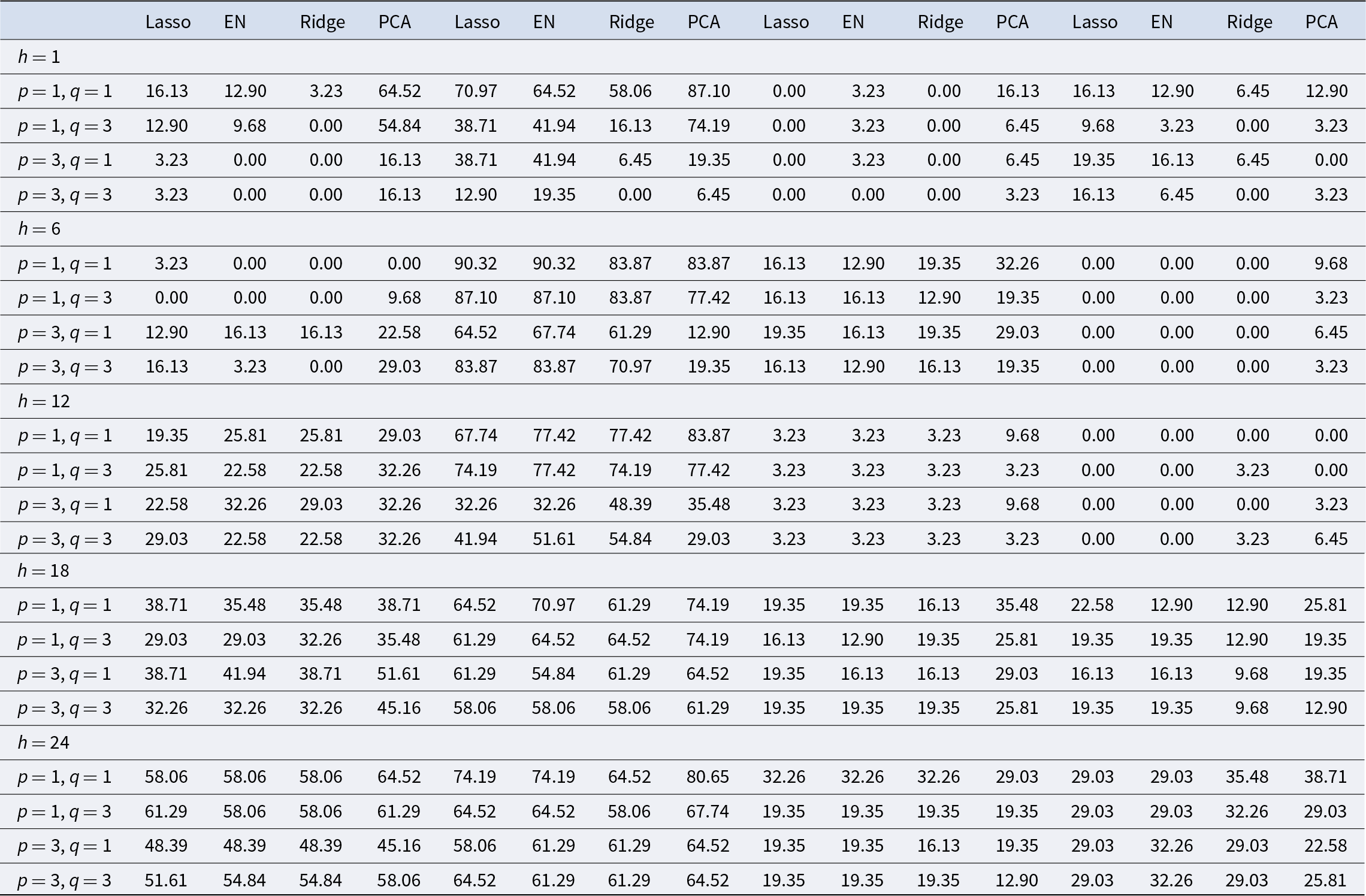
Note: For each forecasting horizon, estimation method, choice of lags in equation (2), and wine index, the table reports the percentage of models (or combination of models) that have an RMSE smaller than benchmark model BM2.
Appendix C

Figure 2. Heatmap for the score ratios. Index: Liv-ex Fine Wine 100. Method: Lasso, Benchmark: BM1.

Figure 3. Heatmap for the score ratios. Index: Retail. Method: Lasso, Benchmark: BM1.

Figure 4. Heatmap for the score ratios. Index: Liv-ex Fine Wine 100. Method: Lasso, Benchmark: BM2.

Figure 5. Heatmap for the score ratios. Index: Retail. Method: Lasso, Benchmark: BM2.

Figure 6. Heatmap for the score ratios. Index: Wholesale. Method: Lasso, Benchmark: BM2.

Figure 7. Heatmap for the score ratios (combined forecasts). Index: Wholesale. Method: Lasso, Benchmark: BM2.


 Open access