


The insurance contracts offered through market and nonmarket mechanisms are important strategies for households to smooth their consumption in the face of idiosyncratic shocks. A collapse of consumption smoothing impedes human capital accumulation and the demographic structure itself, especially in developing economies (Foster Reference Foster1995; Rose Reference Rose1999; Gertler and Gruber Reference Gertler and Gruber2002; Dercon and Krishnan Reference Dercon and Krishnan2002). Therefore, households’ risk-coping behavior has been widely studied ever since a series of pioneering studies provided a systematic empirical design to test consumption smoothing (Rosenzweig Reference Rosenzweig1988; Mace Reference Mace1991; Cochrane Reference Cochrane1991).Footnote 1
In the past, risk-sharing institutions and self-insurance behavior also played an important role in allowing working-class households to cope with idiosyncratic shocks during periods of economic development.Footnote 2 This study systematically investigates the risk-coping behavior of working-class urban households. To do so, I digitize a detailed monthly longitudinal budget survey on factory worker households conducted after WWI in Osaka, the second largest city in Japan.Footnote 3 Utilizing an empirical design that exploits the within variations in the households’ consumption and income, I estimate the income elasticity to determine the extent of consumption insurance. The result indicates that the factory worker households could not fully deal with idiosyncratic shocks. Their income elasticity of total consumption expenditure is found to be comparable to that of urban households in developing countries at the same development stage. Nonetheless, the income elasticities of consumption by subcategory suggest that they might have mitigated the fluctuations in indispensable consumption to some degree. While the elasticities for luxury categories such as furniture, clothes, and entertainment expenses were greater, payments for a few indispensable categories such as food and housing were clearly inelastic. I also provided evidence suggesting that savings institutions helped mitigate idiosyncratic shocks. The households precautionarily saved the surplus built up and relied more on withdrawals from savings than borrowing when they faced the shocks. Temporary income from borrowing, particularly from pawnshops, as well as from the additional labor supply of the wife and child had also played a role among relatively vulnerable households.
This current study contributes to the literature in the following two ways. First, it contributes to the historical literature by adopting a systematic empirical design to test risk-sharing, which can be used in future economic history studies. Different types of analytical specifications have thus far been applied in the field of economic history, which makes comparing the degrees of risk sharing in different countries and eras complicated. In the current study, I employ a standardized empirical design to test risk-sharing (Cochrane Reference Cochrane1991) and compare the estimated income elasticities with those in modern developing societies.Footnote 4 The degree of consumption smoothing can reflect the maturity of insurance markets in a given economy (Dercon Reference Dercon2004). Therefore, applying this approach to other historical panel datasets will offer comparable estimates for a diverse range of economies.
Second, the current study uses a household-level monthly expenditure panel dataset. Since the concept of consumption smoothing pertains to the dynamics of household behavior over time, panel data on household budgets are preferable to test households’ smoothing behavior (Mace Reference Mace1991). However, most previous economic history studies have used cross-sectional data rather than panel data.Footnote 5 To bridge this gap, I use monthly variations in the household budget to investigate risk-coping behavior among working-class households. Relatedly, Japan is a suitable country for investigating risk-coping behavior for the following reasons. While national health insurance schemes expanded in many European countries between the end of the nineteenth century and the early twentieth century, Japan did not establish such a scheme until the mid-twentieth century (Bowblis Reference Bowblis2010). In addition, while the prevailing fragile labor contracts resulted in high turnover rates among factory workers, the unemployment insurance bill was not passed until the late twentieth century. Therefore, idiosyncratic income shocks cannot be compensated by public insurance schemes. This feature of prewar Japan offers an ideal environment for studying consumption-smoothing responses to idiosyncratic income shocks.
The remainder of this paper is organized as follows. The second section briefly reviews the historical context and explains the risk-coping devices. The third section introduces the data used and discusses the sample characteristics. The fourth section empirically analyzes consumption smoothing, and the fifth section assesses risk-coping mechanisms. The final section concludes.
BACKGROUND
The Nature of Risk
In early twentieth-century Japan, employment contracts were typically fragile and stipulated no fixed term of employment; thus, the labor mobility of factory workers, comprising not only unskilled workers but also skilled workers, was extremely high (Moriguchi Reference Moriguchi2000). After WWI, large companies began to introduce comprehensive corporate welfare programs for factory workers to accumulate firm-specific human capital, and the Retirement Allowance Fund Law of 1936, which obligated employers to set up a retirement allowance fund for their employees, complemented these enterprise-based welfare programs (Moriguchi Reference Moriguchi2003). As a result, the average annual turnover rates of large companies began to decline after the war and fell to below 10 percent in the late 1920s (Hyodo Reference Hyodo1971).
However, the factory workers employed by such large companies comprised only about 20 percent of all production workers in the late 1920s (Moriguchi Reference Moriguchi2003, p. 644). Additionally, the average annual turnover rate of small and medium-sized enterprises was still approximately 30 percent (Hyodo Reference Hyodo1971; Taira Reference Taira1970). Therefore, except for a few favored workers among large companies, worker uncertainty in the labor market was high in interwar Japan, a period in which no comprehensive social security system had yet been established (Odaka Reference Odaka, Okazaki and Okuno-Fujiwara1999).Footnote 6
In addition to unemployment, sickness and injury could be another source of uncertainty for workers. The Factory Act of 1916 included an article setting an allowance for workers taking medical leave. In reality, however, most of the factories subject to the Act did not fully compensate workers who took medical leave.Footnote 7 Moreover, because the Act applied only to factories with 15 or more workers, workers in many small factories were entirely neglected.Footnote 8 Thus, sicknesses and injuries might have caused a certain reduction in factory workers’ incomes.
Despite these uncertainties, Japan’s economic growth remained stable during the interwar period (Nakamura Reference Nakamura1981). Inequality among members of the working class, measured in terms of the Gini coefficient, decreased between the early 1920s and early 1930s (Yazawa Reference Yazawa2004; Bassino 2006). Consequently, representative measures of human and physical capital accumulation, such as average years of education and children’s height, climbed steadily during this period.Footnote 9 These developmental outcomes suggest that working-class households might have coped with the risks to a certain extent.
Risk-Coping Devices
SAVINGS INSTITUTIONS
Precautionary savings are an important primary risk-coping device (Deaton Reference Deaton1991; Carroll Reference Carroll1997; Carroll, Dynan, and Krane Reference Carroll, Dynan and Krane2003). In prewar Japan, postal savings (yūbin chokin) and savings banks (chochiku ginkō) were widely used saving institutions around 1920 (Okazaki Reference Okazaki and Saito2002; Tanaka Reference Tanaka2012). In Osaka city, there were 117 postal savings offices and 55 savings banks in 1920. The number of people with postal savings and savings bank accounts was reported to be 725,642 and 1,648,150, respectively, accounting for approximately 60 percent and 130 percent of the number of citizens measured in the census.Footnote 10 Although the statistics must double count people having multiple accounts, they suggest that a large proportion of workers had savings accounts. Average savings per manufacturing worker were roughly 50 yen and 35 yen in postal savings and savings banks in 1920, respectively, approximately equivalent to 30–50 percent of the average monthly income of urban factory workers.Footnote 11 This implies that, despite having only small amounts of savings, factory workers might have drawn on their savings in the event of economic hardship, as suggested by James and Suto (Reference James and Suto2011).Footnote 12
Another type of savings institution was a mutual loan association (mujin), in which members deposited a fixed amount of money into a unit and withdrew it according to certain association rules. However, the association distributed deposits to members using either lotteries or bidding. This means that members could not withdraw the right deposits at the right time. In addition, a large deposit per unit (usually 100–300 yen) meant most members of mujin were probably owners of small businesses, such as merchants.Footnote 13 Moreover, less than 2 percent of the working population in Osaka in 1915 invested money in this way (Osaka City Office 1934, p. 251). In this light, unlike postal savings and savings banks, mutual loan associations were not useful risk-coping devices for factory workers, a large and growing proportion of the urban population.
LENDING INSTITUTIONS
Urban working-class households in prewar Japan could access a few lending institutions.Footnote 14 Among these, pawnshops (shichiya) were the most popular lending institutions, especially among factory workers.Footnote 15 Shibuya, Suzuki, and Ishiyama (Reference Shibuya, Suzuki and Ishiyama1982) argued that factory workers were the most frequent users of pawnshops in cities for a few main reasons (pp. 328–338). First, pawnshops were easier to access than other lending institutions because lenders did not need to check the credit of borrowers. Furthermore, since inexpensive clothes were the most common pawns at that time, workers could borrow money without the risk of falling into heavy debt. Second, the interest rates at pawnshops were relatively low, as they were regulated by the Pawnbroker Regulation Act of 1895. Accordingly, the redemption rate was substantially high: approximately nine out of 10 borrowers could repay their loans within the short term, which enabled them to minimize their interest payments. Finally, physical accessibility was sufficiently high because the number of pawnshops was substantially greater than that of other lending institutions, such as mutual loan associations and usuries.Footnote 16
In Osaka city, pawnshops were regarded as a major lending institution among factory workers (Osaka City Office 1920, p. 153). Of the 983 pawn shops in October 1919, factory workers accounted for 60 percent of all users and 43 percent of the borrowing.Footnote 17 More than 80 percent of those loans were from clothes and the redemption rate was approximately 95 percent.Footnote 18 The average amount borrowed by factory workers per event was 11 yen, accounting for roughly 10 percent of the mean monthly income of factory workers at that time. These amounts suggest that those households used pawnshops to smooth their consumption when they faced idiosyncratic shocks rather than to buy luxury goods or invest, which would require much higher borrowing.
Money lenders (kinsen kashitsuke gyō) also existed in this period (Osaka City Office 1934, pp. 182–183). In 1926, there were 196 money lenders, but the number of lending events per lender was only 118, substantially smaller than that of pawnshops (i.e., approximately 4,000 pawns per shop in the same year). Furthermore, while the average loan amount per pawn was usually 5–10 yen in pawnshops, this figure was substantially large for money lenders at slightly under 300 yen, approximately three times the average monthly household income of factory workers.Footnote 19 This means that money lenders were predominantly used by business owners, such as the owners of small enterprises, merchants, and landowners (Shibuya Reference Shibuya2000, pp. 184, 248). Indeed, by the early 1920s, most money lenders had become usuries (kōrigashi).Footnote 20 Since usuries expected to siphon money from those guarantors rather than the borrowers themselves, three or more joint guarantors with credibility were required to access those lenders. This feature made it harder for the working class to use usuries.
Finally, the main customers of ordinary banks and credit unions (shinyō kumiai) at that time were companies, including other banks. In 1920, there were 24 ordinary banks, with an average loan amount of approximately 27 thousand yen; further, a large part of their collateral was stock certificates.Footnote 21 Although the 24 credit unions might have been accessible to workers, their 4,451 members accounted for only 0.4 percent of the working population in Osaka city in 1926 (Osaka City Office 1934, p. 276).
INFORMAL INSURANCE PROVIDED BY NETWORKS
Evidence on rural economies in today’s developing countries has highlighted the importance of informal networks (e.g., gifts from friends and family) for coping with idiosyncratic shocks because formal insurance markets rarely exist in village economies (Rosenzweig Reference Rosenzweig1988).Footnote 22 Systematic statistics on gifts from personal networks in prewar Japan are unavailable. However, a survey of 185 factory worker households in Tokyo city and surrounding suburban municipalities in November 1922 found that the average monthly income from personal networks was 2.9 yen, accounting for 2.8 percent of total monthly income (Social Affairs Division 1925, pp. 58–59).Footnote 23 This suggests that using temporary income from personal networks might have been a useful strategy for urban factory worker households.
LABOR SUPPLY ADJUSTMENTS
The traditional and still prevalent view of the labor supply among urban working-class households in prewar Japan is the male breadwinner model. In that period, the wife’s elasticity of labor supply was considerably low, and children rarely worked compared with the extensive use of child labor during the Industrial Revolution in Europe (Saito Reference Saito1995, Reference Saito1996; Chimoto Reference Chimoto2012). However, a cross-sectional analysis of poor households in Tokyo found a negative correlation between the income of the household head and the working status of children aged 15 years and older (Yazawa Reference Yazawa2004, p. 315). Although this is a suggestive result, one must be careful about the fact that all existing studies have relied on cross-sectional data, meaning that the dynamic compensating responses to idiosyncratic shocks to the household head’s earnings have not yet been investigated. Considering this, I quantify the labor supply of the wife and children in response to shocks to the income of the household head in the fifth section.
To summarize, working-class households were able to use formal and informal risk-coping strategies. Although informal insurance via private networks is not documented as a separate income category, I consider three categories (i.e., withdrawals and gifts, borrowing, and labor supply adjustments) when I evaluate those strategies in the fifth section. I do so using the best available household-level longitudinal budget dataset, which I will introduce in the following section.
DATA
The Sample
I compiled the data on the monthly budget of working-class households between July 1919 and July 1920 from the Report of Labor Research (RLR).Footnote 24 In this survey, the Municipal Bureau of Labor Research of Osaka investigated the monthly income and expenditure of 411 wage-earning and salaried workers in the Osaka city area. Although the details of the sampling method were not recorded, as is the case with other historical household survey datasets, households were selected through a labor union or directly at factories. To investigate the features of the sample, I compare the occupations among household heads within RLR households with statistics obtained from the national population census. As shown in Column (1) of Panel A in Table 1, only 14 percent of men in the workforce across Osaka prefecture worked in the agricultural sector, compared with the national figure of 46 percent. Column (2) also indicates that 90 percent of working men in Osaka city worked in the manufacturing, commerce, and transportation industries, compared with the national figure of 40 percent.Footnote 25 This reflects that Osaka was an industrialized city and a nice setting to study the consumption decisions of industrial workers. In the RLR dataset, information on the household head’s occupation can be obtained for 406 of the 411 households. Column (3) shows that these heads mainly worked in the manufacturing industry; 83 percent were factory workers.
Table 1 SAMPLE CHARACTERISTICS: COMPARING THE RLR SAMPLE WITH THE CENSUS

Notes: Panel A summarizes the industrial structures measured in the 1920 population census and RLR households. Occupations are classified using the industrial classification of the first population census conducted in 1920. The figures in Column (3) are based on information on the 406 RLR household heads’ occupations. The five household heads whose occupations are classified as “unknown” are not included. Panel B sorts the adult male factory workers in Osaka city in 1920 and heads of the 237 RLR households by the five sectors in the manufacturing industry. Column (1) lists the percentage share of adult male factory workers in each sector. Column (2) shows the mean monthly income of adult male factory workers. The monthly income is calculated as the monthly earnings plus the monthly equivalent bonus. See Online Appendix B.2 for the finer details. Column (3) lists the percentage share of the household heads in each sector. The sample excludes observations with no identifiable sector. Column (4) shows the mean value of the household head’s monthly income.
Sources: Figures for the RLR households are calculated by the author from the Municipal Bureau of Labor Research of Osaka (Reference Tada1919–1920). Industrial structures in Panel A are from the Statistics Bureau of the Cabinet (1928, pp. 8–11) and (1929a, pp. 84–85, 108–109). The occupational structure and earnings in Panel B are from Osaka City Office (1921, pp. 8(44)–8(45); 1922, pp. 8(46)–8(47)).
Considering this feature of sampling, the current study targets only factory-worker households. I first extracted households whose heads worked in factories during the survey period.Footnote 26 Correspondingly, 335 of the original 411 households remain. I then excluded the 18 households lacking information on monthly income or family structure. Further, 78 households were dropped because they were observed for only one month during the survey period. Finally, two households were dropped on account of having reported unrealistic income and expenditure values (i.e., exceeding 500 yen per month). Accordingly, data on 237 factory-worker households were used in the empirical analyses.Footnote 27
The mean household size of the RLR sample is 4.00, whereas that of the factory worker households in the manufacturing industry of Osaka city taken from the population census is 3.99. Hence, my sample does not contain outliers or otherwise unusual household size values. Column (1) in Panel B of Table 1 shows the percentage share of adult male factory workers in each manufacturing sector in Osaka city in 1920, and Column (3) lists the percentage share among RLR household heads. The heads are more likely to work in the machine sector than in other sectors, consistent with the descriptions in the original RLR document. Column (2) lists the average monthly income of adult male factory workers,Footnote 28 whereas Column (4) lists the average monthly income of the household heads in the RLR sample. Clearly, the average monthly income of adult males is close to the monthly income of the RLR heads in each sector.Footnote 29 In addition, the average monthly incomes of adult males and the monthly incomes of the heads show similar figures across different sectors. Both support the evidence that the disproportion in the occupation structure in the RLR sample does not lead to an upward income bias and that the RLR sample approximates the average factory worker in the manufacturing sector in Osaka city.Footnote 30 Even if there are some differences with other factory workers, or with the laboring population remain, the RLR sample provides a rare opportunity to study consumption and risk-coping strategies in an industrializing economy.Footnote 31
Variables
The key data used in this study are monthly household consumption and income. The RLR reports 10 consumption subcategories: food, housing, utilities, furniture, clothes, education, medical, entertainment, transportation, and miscellaneous. These consumption variables are mainly used to estimate the income elasticities in the fourth section. Other expenditures are divided into tax payments, liquidation of loans, and deposits into savings. On the contrary, income is divided into six categories: head, wife, child, other,Footnote 32 borrowing, and miscellaneous. The borrowing category includes money from lending institutions, while the miscellaneous category includes money from savings withdrawals and gifts (Municipal Bureau of Labor Research of Osaka Reference Tada1921, pp. 22–27). Therefore, I rename the miscellaneous category, calling it withdrawals and gifts (not divisible). These income variables are used in the mechanism analysis in the fifth section.
The quality of the data is considered to be sufficiently high to conduct quantitative analyses. The investigators visited all households and instructed them all once or twice per month to check the account books and maintain the quality of the survey (Tada Reference Tada1991a, pp. 11–12). Hence, lazy respondents were unlikely to simply copy and paste entries rather than record each purchase. If this sort of repetition did occur, however, the reported expenses would take the same values during the survey period. To test this potential issue, I check whether the first-differenced values of food expenses have sufficient variation for all the households. The food category is the most useful category for this exercise because it requires careful bookkeeping to sort many grocery items; further, expenditure on food has the largest share of the total as well as large variations due to seasonality and price changes.Footnote 33
I find that the observations of three households take the same values across two consecutive months, accounting for only 0.16 percent of all observations. This supports the evidence that measures of consumption are less likely to contain measurement errors.
Trends
Figure 1a illustrates the rising monthly income and expenditure during the sample period. These trends are consistent with the increasing living standards after WWI (Nakamura and Odaka Reference Nakamura, Odaka, Nakamura and Odaka1989, pp. 36–37). One may wonder whether this upward trend in income suggests that households had more savings or less debt and thus were better able to deal with shocks. However, moderate inflation during the sample period partially canceled out the benefit of the upward trend.Footnote 34 Moreover, Figure 1a indicates that both income and expenditure decreased after April 1920. This trend reflects the recession that followed the war after March 1920 in Japan (Takeda Reference Takeda, Kanji, Akira and Haruhito2002, pp. 9–11). Therefore, my sample period includes expansions and recessions, which should offer an ideal setting within which to analyze the risk-coping behavior of households.
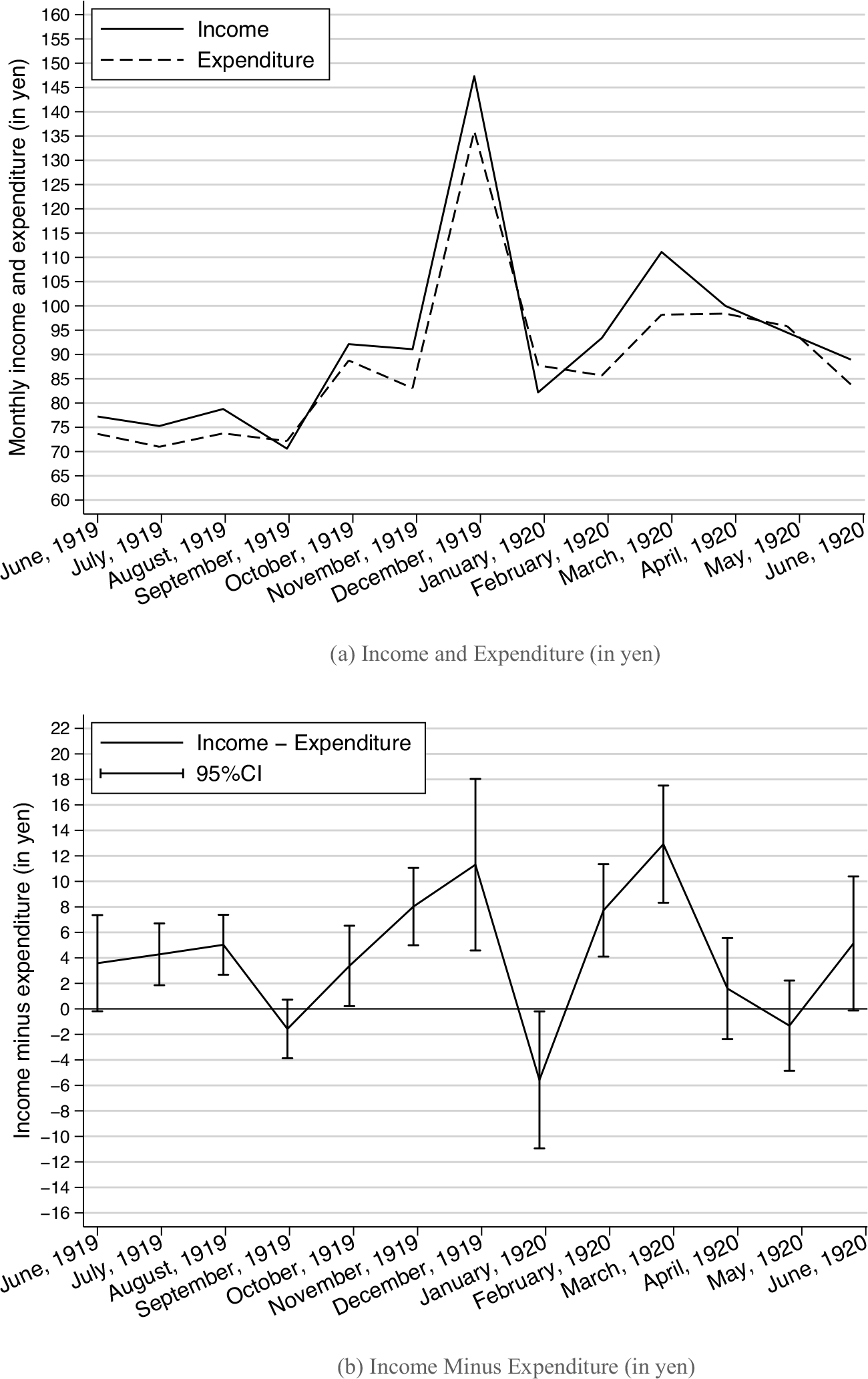
Figure 1 MONTHLY INCOME AND EXPENDITURE BETWEEN JUNE 1919 AND JUNE 1920
Notes: Monthly income and expenditure are illustrated in Figure 1a. The difference between monthly income and monthly expenditure is shown in Figure 1b.
Sources: Created by the author from the Municipal Bureau of Labor Research of Osaka (Reference Tada1919–1920).
Next, I examine the seasonality and variation of idiosyncratic shocks. Figure 1b shows monthly income minus expenditure. Seasonality is clearly observed in December 1919 and January 1920: both income and expenditure increase steeply in December, when bonuses have been paid (Tada Reference Tada1991b, p. 9).Footnote 35 Although the differences between income and expenditure were largely positive but fluctuating, this difference became statistically significant and negative in January because labor income and consumption expenditure typically increase in December to prepare for New Year events and traditions. Workers also took New Year holidays, which could have reduced their earnings. Figure 2 illustrates the box-and-whisker plots of the residuals from the regression of the first-differences in household income on the first-differences in aggregate income, approximating the variations in idiosyncratic shocks during the sample period.Footnote 36 In the figure, the idiosyncratic shocks were clearer in those months in which the net income (i.e., income minus expenditure) exhibited large fluctuations (Figure 1b). Further, the shocks were relatively large in March and April, that is, soon after the recession began.
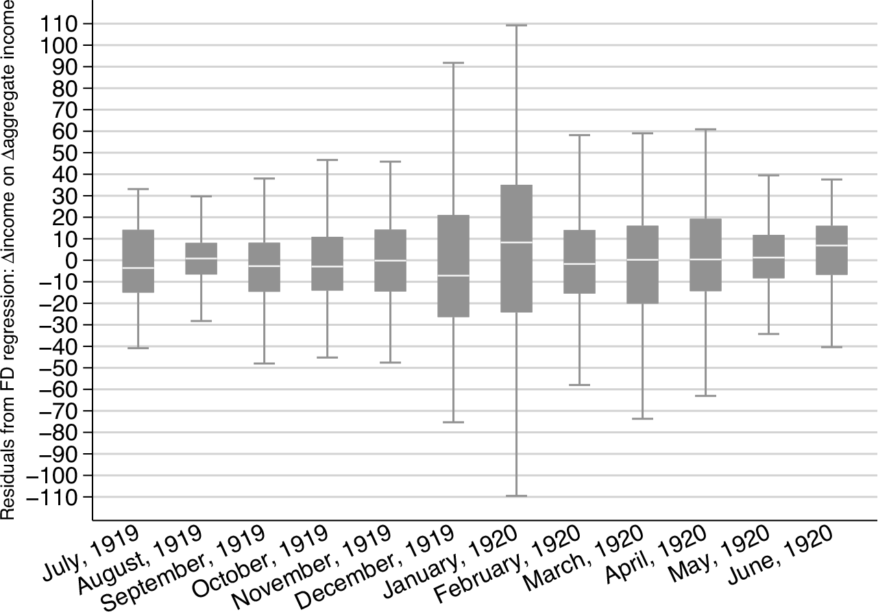
Figure 2 VARIATIONS IN IDIOSYNCRATIC SHOCKS (IN YEN)
Notes: This figure shows the box-and-whisker plot of the residuals from the regression of the first-difference in income on the first-difference in aggregate income. The 25th, 50th, and 75th percentiles are the bottom, middle (white line), and top of the box, respectively. The caps at the ends of the whiskers show the lower and upper adjacent values, respectively.
Sources: Created by the author from the Municipal Bureau of Labor Research of Osaka (Reference Tada1919–1920).
CONSUMPTION SMOOTHING
Estimation Strategy
I begin my analysis by investigating whether risk was shared and which categories of consumption were robust to shocks. Following Cochrane (Reference Cochrane1991) and Ravallion and Chaudhuri (Reference Ravallion and Chaudhuri1997), the empirical specification for household i in time t can be characterized as follows:
 $${\rm{log}}\;{c_{i,t}} = \theta {\rm{log}}\;{y_{i,t}} + x_{i,g,t}^\prime \psi {\rm{ + }}{\mu _{\rm{i}}}{\rm{ + }}{\phi _{\rm{t}}}{\rm{ + }}{u_{{\rm{i}},{\rm{t}}}},$$
where c
i,t
is consumption, y
i,t
is disposable income, µ
i
is the household fixed effect, φ
t
is the month-year fixed effect, and u
i,t
is a random error term.Footnote
37
Household-specific unobservables, such as permanent income and time-constant preferences, are captured by the household fixed effect. In addition, macroeconomic shocks and trends, including seasonality, are controlled for using the month-year fixed effect. Evidence suggests that the households had not lost their heads but had maintained their size during the sample periods. This means that unobservable preference shifts in household consumption do not disturb my results (see Online Appendix C.1 for details).Footnote
38
To be conservative, however, I consider the family size variables interacted with the quarter dummies to control for the potential preference shifts:
 $${x_{i,{g_t}}}$$
is a vector of the controls, where
$${x_{i,{g_t}}}$$
is a vector of the controls, where
 $${g_t} \in \left\{ {1,{\rm{\;}}2,{\rm{\;}}3,{\rm{\;}}4} \right\}$$
is the group membership variable indicating the quarters. Note that the family size controls are interacted with the quarter dummies because these variables are surveyed once in the initial period (Panels A and C of Table 2 show the summary statistics).Footnote
39
If idiosyncratic income shocks are perfectly insured, the coefficient on the change in the growth rate of individual income must be zero. Therefore, the income elasticity captured as the estimate of θ ranges from zero (full insurance) to one (absence of insurance).
$${g_t} \in \left\{ {1,{\rm{\;}}2,{\rm{\;}}3,{\rm{\;}}4} \right\}$$
is the group membership variable indicating the quarters. Note that the family size controls are interacted with the quarter dummies because these variables are surveyed once in the initial period (Panels A and C of Table 2 show the summary statistics).Footnote
39
If idiosyncratic income shocks are perfectly insured, the coefficient on the change in the growth rate of individual income must be zero. Therefore, the income elasticity captured as the estimate of θ ranges from zero (full insurance) to one (absence of insurance).
Table 2 SUMMARY STATISTICS: SAMPLE OF RLR HOUSEHOLDS

Notes: Panel A: Summary statistics for all 237 RLR households. Disposable income is income excluding tax payments. Panel B: Summary statistics for the 202 households that received any income from withdrawals and gifts are listed in Panel B-1. The summary statistics for the 65 households that received any income from borrowing are listed in Panel B-2. Disposable income is income excluding tax payments, temporary income from borrowing, and withdrawals and gifts. Summary statistics for the 194 households with three or more family members (i.e., households with children) are listed in Panel B-3. Panel C: Summary statistics of the family size control variables for all 237 RLR households are listed. The group of children aged 0–5 (%) is used as the reference group in the regression analysis.
Sources: Calculated by the author from the Municipal Bureau of Labor Research of Osaka (Reference Tada1919–1920).
Results
To gain some insights on consumption smoothing, I begin by investigating the raw relationships between the changes in consumption and income. Online Appendix Figures B.2a and B.2b show the distributions of the log-differences in monthly disposable income and expenditure, respectively. Changes in the log of disposable income range from approximately –2.5 to 2.0, whereas changes in the log of expenditure range from approximately –1.5 to 1.5. This finding suggests that income shocks are buffered to some degree. An important fact here is that these idiosyncratic shocks are short-run (temporary) rather than long-run (persistent). Indeed, most households that faced declining disposable income recovered the next month, suggesting that these shocks are caused by temporary sickness and/or layoffs as opposed to chronic diseases or long-term unemployment. This feature of idiosyncratic shocks helps me examine the short-run responses of households.Footnote 40 Online Appendix Figure B.2c describes the relationship between the log-differences in monthly expenditure and disposable income, which shows a positive linear relationship. To delve into this relationship, Figure 3 decomposes total expenditure into the 10 subcategories in Panel A in Table 2, suggesting similar positive relationships between changes in income and most of those subcategories. However, the relationships are rather unclear for housing and education expenditure, implying that some subcategories are less prone to being affected by income shocks.

Figure 3 RELATIONSHIP BETWEEN THE CHANGES IN DISPOSABLE INCOME AND EXPENDITURE
Notes: The relationship between the changes in disposable income and expenditure for the 10 subcategories (Panel A of Table 2) is described in the figures. For comparability, the minimum and maximum values of the y-axis are fixed at –7.0 and 7.0, respectively.
Sources: Created by the author from the Municipal Bureau of Labor Research of Osaka (Reference Tada1919–1920).
Panel A of Table 3 presents the results for Equation (1). For the total consumption category, I find that the estimated coefficient is 0.39 and is statistically significantly different from zero. This implies that a one percent decrease in income results in a 0.39 percent decrease in consumption. Thus, this result suggests that the risks were not perfectly insured, but they might have been partially mitigated. While comparable estimates for urban working-class households in developing economies are scarce, Townsend (Reference Townsend1995) estimated an income elasticity of approximately 0.4 in Bangkok in Thailand between 1975 and 1990. Given that the average standard of living was in a similar range in both cases, this similarity is considered to be plausible.Footnote 41 By contrast, Townsend (Reference Townsend1994) found much smaller estimates (less than 0.14) in Indian villages between 1975 and 1984. Skoufias and Quisumbing (Reference Skoufias and Quisumbing2005) also reported that the income elasticities of consumption were in a similar range in rural areas of Bangladesh, Ethiopia, and Mali in the 1990s (less than 0.15).Footnote 42 This implies that households in village economies are more likely to have access to informal insurance provided by networks, presumably through their familial relationships, than urban households.Footnote 43 However, directly comparing the income elasticity of urban economies with that of rural economies is practically difficult because village households can use self-consumption to mitigate idiosyncratic shocks, which tend to cause a downward bias in consumption. Ravallion and Chaudhuri (Reference Ravallion and Chaudhuri1997) present much greater estimates (approximately 0.5) by revising the bias in Townsend’s (1994) estimates due to such measurement errors in consumption data. This suggests that better access to savings and lending institutions, which is difficult for village households, can be important for mitigating idiosyncratic shocks. While the urban-to-rural comparison of income elasticities is beyond the scope of this study, this debate indicates that research is required to understand risk-sharing behavior in developing economies. In this light, the result provides the first benchmark estimate of income elasticity for any working-class household in the early phase of industrialization.
Table 3 RESULTS OF ESTIMATING INCOME ELASTICITIES

* = Signficant at the 10 percent level.
** = Signficant at the 5 percent level.
*** = Signficant at the 1 percent level.
Notes: This table shows the results of Equation (1): the regressions of the 11 measures of log-transformed consumption on log-transformed disposable income as well as on the family size controls, household fixed effects, and month-year fixed effects. The family size controls are interacted with the quarter dummies. The estimated coefficients on log-transformed disposable income are listed in the second column (Coef.). Panel A reports the estimates from the regressions using 237 households from June 1919 to June 1920. Panel B-1 reports the estimates from the regression using the 86 households with children aged 6–12 from June 1919 to June 1920. Panels B-2 and B-3 report the estimates from the regressions using the 82 households with children aged 6–12 from June 1919 to March 1920 and June 1919 to March 1920, excluding August 1919, respectively. Standard errors in brackets are clustered at the household level.
Sources: Calculated by the author from the Municipal Bureau of Labor Research of Osaka (Reference Tada1919–1920).
The estimates of the 10 subcategories in Panel A of Table 3 are statistically significantly positive in most cases. Overall, the elasticities are greater for “luxury” categories such as furniture (0.66), clothes (0.68), and entertainment expenses (0.55). On the contrary, they are relatively small for the other subcategories; those for food, housing, education, medical expenses, and transportation are smaller than the elasticity for total consumption (0.39). Specifically, as I show in a descriptive manner in Figure 3, the estimates of housing and education are particularly inelastic and even statistically insignificant at the critical level of 5 percent. The result for housing may not be surprising given that rent needs to be paid regardless of fluctuations. Indeed, since most landlords of rental houses in cities leased land from landowners, they should have paid ground rent (Kato Reference Kato1990, pp. 79–80). This feature led to rental trouble for the working class around 1920, including evictions (Ono Reference Ono1999, pp. 48–49).
By contrast, the result for education may need further clarification. I first trim the sample to the 86 households that have children aged 6–12. As Panel B-1 of Table 3 shows, the estimate for education is close to zero and statistically insignificant. Next, I remove the potential impacts of graduation on education expenditure. Because Japan’s academic year starts in April and ends in March, some children might have graduated from school at the end of March 1920, which would disrupt education expenditure. To address this issue, I run a regression using an alternative cut-off period between June 1919 and March 1920, as shown in Panel B-2 of Table 3. In the same way, I exclude August 1919 to deal with potential fluctuations due to the summer holiday, as shown in Panel B-3 of Table 3. The results remain unchanged, suggesting that graduation and open seasonality do not affect the findings.
Mean monthly education expenses per child among RLR households with children aged 6–12 are 0.44 yen, considerably lower than other expenses such as clothes, whose per-capita mean is 1.94 yen in those households. After the Order of Primary School (shōgakkō rei) was revised in 1900, primary school was regarded as compulsory education, and tuition fees declined throughout the early twentieth century (Hijikata Reference Hijikata2002). Indeed, average tuition spending was only 0.18 yen per month in Osaka city in 1920, accounting for less than 0.2 percent of the average monthly income of the households analyzed.Footnote 44 Consequently, withdrawals for economic reasons rarely occurred by the 1920s (Hijikata Reference Hijikata2002, p. 32).Footnote 45 This institutional advantage may explain my results.Footnote 46 However, my result for education may be influenced by the data frequency: one can expect less insurance at the monthly level than annually because the consumption of some goods can be delayed in the short term (Nelson Reference Nelson1994). In this light, education could be more of a long-term decision for parents. Thus, one must be careful in concluding that RLR households kept children in education despite idiosyncratic shocks.
Nakagawa (Reference Nakagawa1985) contended that urban factory worker households in the early twentieth century kept spending on miscellaneous payments other than food to maintain their household (p. 379). His argument is based on comparing expenditures on certain consumption categories calculated from several survey reports measured in different years. Despite the methodological differences, my results for food and housing expenses are consistent with his argument. Importantly, I also find that the income elasticities are positive in most consumption subcategories and that their magnitudes vary by category: payments for indispensable items such as food and housing are more likely to be inelastic than those for luxury items such as clothes and furniture.Footnote 47
RISK-COPING STRATEGIES
The foregoing results provide suggestive evidence that the factory worker households smoothed their consumption to some degree. In this section, I investigate whether temporary sources of income such as savings and borrowing served to share risk among households and whether adjusting labor supply helped them cope with shocks.
Savings and Borrowing
ESTIMATION STRATEGY
I derive the empirical specification to test risk-sharing strategies in the spirit of Fafchamps and Lund (Reference Fafchamps and Lund2003). The specification for household i at time t can be characterized as follows:
 $${r_{i,t}} = \kappa + \delta {\widetilde y_{i,t}} + x_{i,{g_t}}^{\rm{'}}\gamma + {\nu _i} + {\zeta _t} + {e_{i,t}}$$
Where
 $${\widetilde y_{i,t}}$$
is disposable income,
$${\widetilde y_{i,t}}$$
is disposable income,
 $${x_{i,{g_t}}}$$
is the family size controls included in Equation (1), νi indicates the household fixed effect,
$${x_{i,{g_t}}}$$
is the family size controls included in Equation (1), νi indicates the household fixed effect,
 $${\zeta _t}$$
indicates the month-year fixed effect, and ei,t is a random error term.Footnote
48
Since the household fixed effect absorbs variations in permanent income as well as the initial endowment of assets, disposable income
$${\zeta _t}$$
indicates the month-year fixed effect, and ei,t is a random error term.Footnote
48
Since the household fixed effect absorbs variations in permanent income as well as the initial endowment of assets, disposable income $({\widetilde y_{i,t}})$
captures the idiosyncratic income shocks in the regression.
$({\widetilde y_{i,t}})$
captures the idiosyncratic income shocks in the regression.
I use several income and expenditure categories for r i,t . First, temporary income from withdrawals and gifts is used to test the role of precautionary savings. I also use monthly deposits to savings to confirm the saving behavior of the households: the signs of the estimates for the withdrawals and gifts and for deposits to savings should be symmetric if the households had precautionarily saved their earnings during good times.Footnote 49 Second, I use temporary income from borrowing and liquidating loans to dually test the roles of lending institutions. One can expect the estimates to be almost symmetric. Finally, I use expenditures on clothes and furniture to test the potential role of pawnshops. Although the borrowing category is indivisible, pawnshops were the most popular lending institutions, and clothes were the dominant article for pawning. Hence, while the estimate for clothes could be sensitive to shocks, that for furniture, a placebo item, should be close to zero and statistically insignificant.
The analytical sample is trimmed to households that received income from either withdrawals and gifts or any borrowing during the sample period.Footnote 50 Panels B-1 and B-2 of Table 2 list the summary statistics.
RESULTS
Panels B-1 and B-2 of Table 2 indicate that households tended to rely more frequently on savings than borrowing (1,023 vs. 154 obs.). This suggests that households regard savings as the first line of defense and borrowing as the second line (Deaton Reference Deaton1991). Given this, I begin my analysis by estimating income elasticity for the savings categories.
Panel A of Table 4 presents the results. Columns (1) and (2) show the estimates for withdrawals and gifts. Columns (3) and (4) show the estimates for deposits to savings. The estimates in Columns (1) and (3) suggest that when households faced negative income shocks, withdrawals and gifts increased, whereas deposits to savings decreased.Footnote 51 To compare the estimate by addressing the attenuation effects induced by censoring, Columns (2) and (4) employ the fixed-effects Tobit model proposed by Honoré (Reference Honoré1992). As expected, the magnitudes become larger in both columns. The estimate for the withdrawals and gifts category is slightly higher than that for deposits to savings (0.46 vs. 0.32). Although inconclusive, as the former income category is indivisible, this margin might suggest the potential contribution of gifts from informal insurance provided by networks (Rosenzweig Reference Rosenzweig1988).
Table 4 RESULTS OF TESTING THE RISK-COPING MECHANISMS

* = Signficant at the 10 percent level.
** = Signficant at the 5 percent level.
*** = Signficant at the 1 percent level.
Notes: The results from the fixed-effects Tobit model, as proposed by Honoré (Reference Honoré1992), are reported in Columns (2) and (4) in each panel. A quadratic loss function is applied for the estimation to ensure computational tractability. Robust standard errors are in brackets. Standard errors are clustered at the household level in the linear models. Panel A presents the results for the savings category: withdrawals and gifts (Columns (1) and (2)) and deposits to savings (Columns (3) and (4)). Panel B presents the results for the borrowing category: borrowing (Columns (1) and (2)) and liquidation of loans (Columns (3) and (4)). Panel C presents the results for expenditure on clothes (Columns (1) and (2)) and furniture (Columns (3) and (4)). All the regressions in each panel include the disposable income, family size controls, household fixed effects, and month-year fixed effects. The family size controls are interacted with the quarter dummies.
Sources: Calculated by the author from the Municipal Bureau of Labor Research of Osaka (Reference Tada1919–1920).
The estimate in Column (2) suggests that a one standard deviation decrease in disposable income increases temporary income from withdrawals and gifts by 16 yen, accounting for roughly 50 percent of the average savings in savings banks of manufacturing workers in Osaka at that time. This finding implies that while precautionary savings served as a primary risk-coping strategy among households, they might not have provided sufficient compensation when households faced a rare but extreme loss of income (e.g., a more than two standard deviation decrease). Despite this, the result for deposits to savings also evokes a serious attribute of urban factory worker households: they saved the surplus built up in good times to prepare for future risks. This finding is consistent with James and Suto’s (2011) historical view of frugal working-class households.
Panel B of Table 4 lists the estimates for the borrowing categories in the same column layout. Columns (1) and (3) suggest that households borrowed money when they faced negative income shocks, whereas they liquidated loans in good times. As expected, the magnitudes become much larger after addressing the censoring issues in Columns (2) and (4). To delve into the mechanism behind the roles of borrowing, I next examine the results for expenditure on luxury items listed in Panel C of Table 4: Columns (1) and (2) for clothes and Columns (3) and (4) for furniture. While the estimates for clothes are weakly statistically significantly positive, the estimates from the placebo test using expenditure on furniture are close to zero and statistically insignificant. This finding seems to be consistent with the historical fact that clothes were the most representative article for pawning at that time, whereas furniture was rarely used, suggesting a role for pawnshops in mitigating idiosyncratic income shocks. Fafchamps, Udry, and Czukas (Reference Fafchamps, Udry and Czukas1998) showed that the ownership of mobile assets such as livestock can be used to mitigate vulnerability to idiosyncratic income shocks in village economies. In this light, my result implies that urban factory worker households in prewar Japan owned clothes as real assets and bought some of those assets in good times, as suggested by Deaton (Reference Deaton1992).
The estimate in Column (2) of Panel B of Table 4 implies that a one standard deviation decrease in disposable income increases temporary income from borrowing by 14 yen. Similarly, the estimate in Column (4) indicates that a one standard deviation increase in disposable income increases liquidation by 12 yen. Given that the average amount borrowed by factory workers per event in pawnshops in Osaka city was 11 yen, these magnitudes are quite reasonable. In other words, urban factory worker households took out loans within their solvencies.
HETEROGENEOUS RESPONSES
These findings suggest that both precautionary savings and borrowing mitigated idiosyncratic income shocks. However, richer households with high precautionary savings may borrow less because they see consumption fluctuations with income as savings run out.Footnote 52 To test such potential heterogeneous responses with respect to borrowing, I stratify the sample based on the median of households’ mean savings expensesFootnote 53 and run regressions for each subsample using Equation (2).Footnote 54 To deal with the attenuations from censoring revealed in Table 4, I use the fixed-effects Tobit estimation in all the regressions.
Panel A of Table 5 presents the results. Columns (1) and (3) show the estimates for withdrawals and gifts for the subsamples below and above the median, respectively. The estimates are statistically significantly negative and have a similar range in both cases. Columns (2) and (4) list the estimates of income from borrowing for the subsamples in the same layout.Footnote 55 The estimate for the subsample with less savings is statistically significantly negative, whereas the estimate for the subsample with more savings is negative but statistically insignificant. The estimate in Column (2) is greater than that in Column (4) in an absolute sense.
Table 5 RESULTS OF TESTING THE RISK-COPING MECHANISMS: HETEROGENEOUS RESPONSES

* = Signficant at the 10 percent level.
** = Signficant at the 5 percent level.
*** = Signficant at the 1 percent level.
Notes: The results from the fixed-effects Tobit model, as proposed by Honoré (Reference Honoré1992), are reported. A quadratic loss function is applied for the estimation to ensure computational tractability. Robust standard errors are in parentheses. Panel A presents the results for the temporary income categories: Columns (1) and (3) for withdrawals and gifts and Columns (2) and (4) for borrowing. The analytical sample used in Panel A of Table 5 is stratified into two subsamples based on the median of households’ mean monthly deposits to savings: Columns (1) and (2) for households lower than or equal to the median (101 and 33 households for Columns (1) and (2), respectively) and Columns (3) and (4) for households higher than the median (101 and 32 households for Columns (3) and (4), respectively). Panel B presents the results for expenditure on clothes and furniture: Columns (1) and (3) for clothes and Columns (2) and (4) for furniture. The analytical sample used in Panel B of Table 5 is stratified into two subsamples by the median of households’ mean monthly income from borrowing: Columns (1) and (2) for the 31 households less than or equal to the median and Columns (3) and (4) for the 34 households more than the median. All the regressions in each panel include the disposable income, family size controls, household fixed effects, and month-year specific fixed effects. The family size controls are interacted with the quarter dummies.
Sources: Calculated by the author from the Municipal Bureau of Labor Research of Osaka (Reference Tada1919–1920).
Panel B of Table 5 assesses whether the results are consistent with the role of pawnshops in the same manner as in Panel C of Table 4. In this panel, I stratify the sample based on the median of households’ mean monthly income from borrowing. Columns (1) and (3) present the estimates for clothes for the subsamples below and above the median, respectively. Income elasticity is statistically significantly positive among households that borrowed more, suggesting they might have stored the clothes in good times. The estimate for households with less borrowing is higher, albeit statistically insignificant. Although this result may partially reflect the income effects for clothes, the large standard error implies that a subset of households in this subsample did not pawn clothes. The placebo results seem to support the potential mechanism via pawning, as shown in Panel C of Table 4, where the estimates for the furniture are closer to zero in both subsamples (Columns (2) and (4)).
These results provide suggestive evidence that, while households regarded savings as a primary risk-coping strategy, borrowing was another option for relatively vulnerable households with less precautionary savings.
Labor Supply Adjustments
The increased dependence on the household head’s earnings due to urbanization could increase demand for market purchases of insurance (di Matteo and Emery 2002). However, additional labor supply could be an alternative means of coping with income shocks (Horrell and Oxley Reference Horrell and Oxley2000; Moehling Reference Moehling2001). In the foregoing regressions, I included family structure variables to control for potential preference shifts and related labor supply adjustments. In this subsection, I explicitly test whether shocks to the income of the household head caused the labor supply to be adjusted.
To create a suitable empirical setting for the test, I trim the sample to households with three or more family members, leaving 194 households, including the head and both the wife and the child(ren). I regress either the wife’s or the child’s income on the income of the household head, family size controls, and household and month-year fixed effects.Footnote 56 As shown in Panel B-3 of Table 2, approximately 20 percent (347/1,627) and 15 percent (244/1,627) of the observations have positive values for the wife’s and child’s incomes, respectively. To deal with this censoring issue, I employ the fixed-effects Tobit estimation and run the wife’s and child’s income equations separately.Footnote 57
Panel A of Table 6 presents the results. Column (1) shows the negative but insignificant estimate for the wife’s income. Column (2) shows the statistically significantly negative estimate for the child’s income.Footnote 58 The percentage of working children indicates that this result should come from children aged 13 years and older (i.e., those who have left primary school).Footnote 59 This finding is consistent with the discussion in the fourth section about the low income elasticity for education expenses. In addition, it is in line with the findings from cross-sectional evidence of urban working-class households in prewar Japan exploiting the labor supply of children aged 15 years and older.
Table 6 RESULTS OF TESTING THE RISK-COPING MECHANISMS: LABOR SUPPLY ADJUSTMENTS

* = Signficant at the 10 percent level.
** = Signficant at the 5 percent level.
*** = Signficant at the 1 percent level.
Notes: The results from the fixed-effects Tobit model, as proposed by Honoré (Reference Honoré1992), are reported. A quadratic loss function is applied for the estimation to ensure computational tractability. Robust standard errors are in parentheses. Panel A shows the results for the 194 households with three or more family members. Panel B stratifies households based on the median of households’ mean monthly deposits to savings. Columns (1) and (2) show the results for the 97 households below the median and Columns (3) and (4) present the results for the 97 households above the median. All the regressions in each panel include the income of the household head, family size controls, household fixed effects, and month-year fixed effects. The family size controls are interacted with the quarter dummies.
Sources: Calculated by the author from the Municipal Bureau of Labor Research of Osaka (Reference Tada1919–1920).
However, my estimates from the subsamples stratified by the median of households’ mean deposits to savings show a different story. Panel B of Table 6 presents the results. Columns (1) and (2) show the results for the subsample below the median, and Columns (3) and (4) show those for the subsample above the median. Among the former, the estimate for the wife’s income is now statistically significantly negative (Column (1)), and that for the child’s income is higher (Column (2)). By contrast, the estimates are not statistically significant among households above the median (Columns (3) and (4)). Compared with the elasticities for savings and borrowing, which are approximately 0.5 and 0.8 (Columns (1) and (2) in Panel A of Table 5), the elasticities of the labor supply of the wife and child (approximately 0.2 and 0.6, respectively) are slightly lower, but still within a similar range. Therefore, adjusting labor supply could have been an important risk-coping strategy among households with less savings. Finally, I confirm that these results are robust to using an alternative definition of the shock variable, namely, an indicator variable for the negative shock on the income of the household head (Online Appendix C.2).
CONCLUSION
Using a systematic empirical design with a unique household-based monthly-level panel dataset, this study is the first to investigate historical consumption smoothing behavior among factory worker households in an industrial city in Japan. The income elasticity estimate of total consumption expenditure provides evidence that factory worker households in Osaka in the 1920s were as vulnerable to idiosyncratic shocks as urban households in the developing world at the same developmental stage, such as Bangkok during the 1970s and 1980s. The estimated elasticities of the consumption subcategories also provide suggestive evidence that while households at that time could not fully cope with idiosyncratic shocks, they mitigated the fluctuations in indispensable consumption. Indeed, the results of the mechanism analysis suggest that while households withdrew their savings as the first line of defense to deal with idiosyncratic income shocks, they saved the surplus in good times to prepare for future risks. Among households with less savings, borrowing, particularly from pawnshops, worked as a second line of defense. The additional labor supply of the wife and child in response to shocks to the income of the household head was also observed in relatively vulnerable households.
The risk-coping behavior among urban factory worker households in prewar Japan documented in this study indicates that they partially coped with idiosyncratic short-term income shocks using available sources of temporary income and adjusting labor supply. To delve into the efficiency of historical insurance markets, it is also valuable to investigate whether the long-term variation in income was insured during historical economic growth. As evidence from developed economies suggests that permanent shocks are far less insured than transitory shocks (Blundell, Pistaferri, and Preston Reference Blundell, Pistaferri and Preston2008), long-term shocks may rarely be insured in historical cases. Despite this, the analyses based on the low-frequency budget data should provide new findings on the long-run risk-coping behaviors of the past.
Although the potential role of informal insurance, such as gifts from relatives and insurance sold in the market, should be investigated in more detail, the results of this study reveal the risk-coping mechanisms and illustrate a much clearer picture of consumption smoothing behavior among urban working-class households than the traditional view. This study provides the first estimates of income elasticities of consumption in the historical setting of working-class households in the first industrializing country in Asia. Given the increasing availability of historical panel data, this study’s estimates could serve as a benchmark for future studies on consumption smoothing behavior in other historical contexts.


