


1. Introduction
Flows through patterned conduits are encountered in numerous technological applications. Large-scale patterns are commonly added for the enhancement of heat and/or mass transfer. Sometimes wall corrugations result from adding ribs to increase the structural robustness of the design. Such surface irregularities alter the flow dynamics and can degrade flow performance by increasing hydraulic losses. The proper design and application of surface patterns can possibly allow us to mitigate undesired effects, increase structural robustness and improve the flow performance, either by increasing mixing through the onset of non-stationary, chaotic (in the Lagrangian sense) motions (Gepner & Floryan Reference Gepner and Floryan2020; Gepner, Yadav & Szumbarski Reference Gepner, Yadav and Szumbarski2020) or by decreasing hydraulic drag (Mohammadi & Floryan Reference Mohammadi and Floryan2010, Reference Mohammadi and Floryan2013; Yadav, Gepner & Szumbarski Reference Yadav, Gepner and Szumbarski2017, Reference Yadav, Gepner and Szumbarski2018, Reference Yadav, Gepner and Szumbarski2021), allowing for energy-efficient designs.
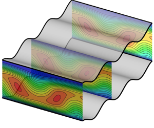
The intent of the current work is to study the dynamics of flows through conduits whose walls have been modified by large, regular groove patterns. The orientation of the grooves can be such that lines of constant elevation run parallel to the flow, forming longitudinal grooves (see figure 1a). The configuration where lines of constant elevation are perpendicular to the flow leads to transverse grooves (see figure 1b). It is known that longitudinal grooves lead to drag reduction (Mohammadi & Floryan Reference Mohammadi and Floryan2010, Reference Mohammadi and Floryan2013; Szumbarski & Błoñski Reference Szumbarski and Błoñski2011; Szumbarski, Blonski & Kowalewski Reference Szumbarski, Blonski and Kowalewski2011) and are subject to a low Reynolds number transition to secondary states driven by an inviscid instability mechanism (Szumbarski Reference Szumbarski2007; Mohammadi, Moradi & Floryan Reference Mohammadi, Moradi and Floryan2015; Yadav et al. Reference Yadav, Gepner and Szumbarski2017; Pushenko & Gepner Reference Pushenko and Gepner2021). They are also subject to transition at higher Re, driven by the classical, travelling Tollmien–Schlichting (TS) wave instability (Moradi & Floryan Reference Moradi and Floryan2014).

Figure 1. Groove direction.
Investigations of flows in conduits with transverse grooves go back to the work of Sobey (Reference Sobey1980) and the extensive experimental investigations of Nishimura and collaborators (Nishimura, Ohori & Kawamura Reference Nishimura, Ohori and Kawamura1984; Nishimura et al. Reference Nishimura, Ohori, Kajimoto and Kawamura1985, Reference Nishimura, Murakami, Arakawa and Kawamura1990a,Reference Nishimura, Yano, Yoshino and Kawamurab). Different forms of transverse grooves have been considered mostly as a method to augment heat and/or mass transfer (Wang & Vanka Reference Wang and Vanka1995; Wang & Chen Reference Wang and Chen2002). Recently, the use of grooves in microchannels was considered as part of an energy harvesting piezoelectric device (Lee et al. Reference Lee, Sherrit, Tosi, Walkemeyer and Colonius2015). Theoretical investigations have been directed at understanding the destabilization mechanisms activated by different variants of such grooves. The most important results include the identification of two types of unstable modes. The first one is the shear-driven travelling wave (Blancher, Creff & Le Quere Reference Blancher, Creff and Le Quere1998; Cabal, Szumbarski & Floryan Reference Cabal, Szumbarski and Floryan2002; Floryan Reference Floryan2005; Asai & Floryan Reference Asai and Floryan2006; Floryan Reference Floryan2007, Reference Floryan2015; Floryan & Floryan Reference Floryan and Floryan2010; Floryan & Asai Reference Floryan and Asai2011; Rivera-Alvarez & Ordonez Reference Rivera-Alvarez and Ordonez2013; Gepner & Floryan Reference Gepner and Floryan2016) that, in the limit of a smooth channel, reduces to the classical TS wave. This mode leads to transition from a stationary to an oscillatory (Stephanoff, Sobey & Bellhouse Reference Stephanoff, Sobey and Bellhouse1980; Ralph Reference Ralph1986), eventually aperiodic (Guzm $\dot{{\rm a}}$n & Amon Reference Guzmn and Amon1994; Blancher et al. Reference Blancher, Creff and Le Quere1998) and chaotic (Guzm $\dot{{\rm a}}$n & Amon Reference Guzmn and Amon1994, Reference Guzmn and Amon1996) flow as the relevant Reynolds number increases. The second instability mode is attributed to the centrifugal forces associated with the groove-imposed changes of the stream direction and is manifested by the onset of stationary, streamwise vortices. Its existence has been documented experimentally (Gschwind, Regele & Kottke Reference Gschwind, Regele and Kottke1995; Mitsudharmadi, Jamaludin & Winoto Reference Mitsudharmadi, Jamaludin and Winoto2012), numerically (Cho, Kim & Shin Reference Cho, Kim and Shin1998) and theoretically (Cabal et al. Reference Cabal, Szumbarski and Floryan2002; Floryan Reference Floryan2002, Reference Floryan2003a, Reference Floryan2007, Reference Floryan2015). It has been shown that the centrifugal mode might play a critical role in channels with a certain class of grooves (Floryan Reference Floryan2007; Floryan & Floryan Reference Floryan and Floryan2010; Gepner & Floryan Reference Gepner and Floryan2016). A similar instability mode has been identified in the channel flow modulated by streamwise-periodic wall transpiration with zero net flux (Floryan Reference Floryan1997, Reference Floryan2003b; Szumbarski Reference Szumbarski2002b).
While the number of possible groove configurations is uncountably infinite, here we focus on the effects of transverse sinusoidal grooves placed on both walls in the in-phase position which results in the formation of a wavy channel (see figures 2 and 3). The flow regimes subject to investigation are limited to moderate Reynolds numbers and the effects of several geometric parameters are examined. The analysis uses direct numerical simulations (DNS) based on a spectral finite-element spatial discretization in the streamwise and wall-normal directions combined with a Fourier decomposition in the spanwise direction as implemented in NEKTAR++ (Cantwell et al. Reference Cantwell2015; Moxey et al. Reference Moxey, Cantwell, Bao, Cassinelli, Castiglioni, Chun, Juda, Kazemi, Lackhove and Marcon2019). A similar approach was successfully used in investigations of stability and nonlinear saturation states by Gepner & Floryan (Reference Gepner and Floryan2016), Yadav et al. (Reference Yadav, Gepner and Szumbarski2017, Reference Yadav, Gepner and Szumbarski2018) and Gepner et al. (Reference Gepner, Yadav and Szumbarski2020).

Figure 2. Shift-symmetry of the geometry.

Figure 3. Sinusoidal channel geometry.
This paper is organized into four parts. First, we study the two-dimensional (2-D), low Reynolds number flows and use the small groove wavenumber approximation to arrive at an analytical formula for the hydraulic losses associated with the corrugations. Second, the dynamics and flow properties of 2-D stationary and oscillatory states are examined for arbitrary wavenumbers. Issues of interest are the onset and growth of the separation zones, the drag penalty associated with groove geometries, and the admissibility of in-, anti- and out-of-phase solutions. The notion of the flow solution being out of phase or either in phase or antiphase is understood here as its ability (or lack of it) to commensurate with the channel's geometry and is schematically illustrated in figure 2. Specifically, considering two consecutive grooves, one at the bottom and the other at the top of the channel, we note that the geometry is symmetric with a shift across the horizontal axis ( $y=0$) and with a shift equal to half of the corrugation wavelength. Flow solution either follows this type of symmetry (is in phase), reverses it (is in antiphase) or shifts spatially to become out of phase. We will examine this in more detail in § 3.1.1. Third, we analyse three-dimensionalization of the flow through the formation of stationary, streamwise vortices. Finally, the nonlinear states resulting from the interaction of the 2-D and three-dimensional (3-D) states are examined, leading to the construction of a bifurcation diagram illustrating possible paths for the flow evolution as the relevant Reynolds number increases.
2. Problem statement
Consider flow of an incompressible, Newtonian fluid forced through a wavy, sinusoidal channel depicted in figure 3. The upper and lower walls of the conduit are located at
 \begin{equation} \left.\begin{gathered} y=y_u=1+S\cos(\alpha x), \\ y=y_l=-1+S\cos(\alpha x). \end{gathered}\right\} \end{equation}
Channel geometry is parametrized by the corrugation wavelength  ${\lambda _\alpha =2{\rm \pi} /\alpha }$, with $\alpha$ being the corrugation wavenumber and the corrugation amplitude $S$ with half of the smooth ( $S=0$) channel opening $h$ used as the length scale. Flow domain extends to ${\pm \infty }$ in the streamwise $x$- and spanwise $z$-directions. Flow evolution is governed by the Navier–Stokes (N–S) and continuity equation,
 \begin{equation} \left.\begin{gathered} \boldsymbol{\nabla} \boldsymbol{\cdot} \boldsymbol{u} = 0,\\ \frac{\partial \boldsymbol{u}}{\partial t}+\boldsymbol{u} \boldsymbol{\cdot} \boldsymbol{\nabla} \boldsymbol{u} =-\boldsymbol{\nabla} p + \frac{1}{Re} \nabla^2 \boldsymbol{u}, \end{gathered}\right\} \end{equation}
where  $\boldsymbol {u}={[u,v,w]}^{\textrm {T}}$ is the velocity vector and $p$ stands for the pressure. Plane Poiseuille flow between flat walls located at $y=\pm 1$ is used as reference – it is characterized by the velocity $\boldsymbol {u}$, the pressure $p$ and the flow rate $Q_r$ of the form
 \begin{equation} \left.\begin{gathered} {u} = [1-y^2, 0, 0],\\ p=-\frac{2x}{Re}, \\ Q_r=\frac{4}{3}. \end{gathered}\right\} \end{equation}
Velocity is scaled with the maximum of the streamwise velocity component of the reference flow  $U_s$, $\rho U_s^2$ is used as the pressure scale, time is scaled with ${h}/{U_s}$ and ${Re={U_s h}/{\nu }}$ stands for the Reynolds number with $\nu$ representing kinematic viscosity. It is assumed that the pressure gradient driving the flow remains constant while the channel morphs into a sinusoidal form. This is equivalent to the imposition of the fixed pressure gradient constraint of the form
 \begin{equation} \left.\frac{\partial p}{\partial x}\right|_{mean} = \frac{-2}{Re}. \end{equation}
The resulting flow rate and the effective Reynolds number (defined either by the maximum or by the bulk velocity) change with geometry and need to be determined a posteriori.
Boundary conditions are the no-slip and no-penetration conditions at the channel walls and periodicity conditions in the streamwise  $x$- and spanwise $z$-directions, with $L_x$ and $L_z$ denoting dimensions of the computational box which must contain an integer number of grooves in the $x$-direction. Boundary conditions can be written in the following form:
 \begin{equation} \boldsymbol{u}=0 \text{ at } \begin{cases} y=y_u, \\ y=y_l, \end{cases}\quad \text{and}\quad \left.\begin{gathered} \boldsymbol{u}(x,y,z)=\boldsymbol{u}(x+L_x,y,z+L_z),\\ p(x,y,z) = p(x+L_x,y,z+L_z). \end{gathered}\right\} \end{equation}
 As the geometry of the channel morphs, the flow acquires new features and eventually bifurcates to a totally new state. We shall use the linear stability analysis to determine the onset conditions marking the formation of new states. In the forthcoming linear stability analysis, we start with a stationary flow solution  $(\boldsymbol {U},P)$ to (2.2) which we acquire via DNS using the numerical procedure outlined below. The flow is than represented as a superposition of this stationary solution and a small amplitude perturbation, i.e. $(\boldsymbol {U_T}, P_T) = (\boldsymbol {U}, P) + (\boldsymbol {u}_{\boldsymbol {p}}, p_p)$, where subscripts $T$ and $p$ stand for total and perturbation quantities. Perturbed quantities are substituted into governing equations (2.2), followed by standard linearization of the perturbation problem. The form of the perturbation $(\boldsymbol {u}_{\boldsymbol {p}}, p_p)$ is restricted to a normal mode form, periodic in the spanwise $x$- and streamwise $z$-direction, and of the form
 \begin{equation} \left.\begin{gathered} \boldsymbol{u}_{\boldsymbol{p}}(x,y,z,t)=\hat{\boldsymbol{u}}_p(x,y)\,{\rm e}^{{\rm i}(\delta x + \beta z -\sigma t)}+{\rm c.c.}, \\ p_p(x,y,z,t) = \hat{p}_p(x,y)\,{\rm e}^{{\rm i}(\delta x + \beta z - \sigma t)}+{\rm c.c.}, \end{gathered}\right\} \end{equation}
where  $\hat {\boldsymbol {u}}_p$ and $\hat {p}_p(x,y)$ are perturbation amplitude functions, c.c. stands for complex conjugate, $(\beta, \delta )$-pair represents the streamwise and spanwise wave numbers (both are real and treated as parameters) and $\sigma =\sigma _r+\textrm {i}\sigma _i$ is the complex amplification rate whose real and imaginary parts correspond to perturbation frequency and growth rate, respectively. The linearized flow problem with perturbation (2.6) leads to a generalized eigenvalue problem for the partial differential equations for the modal functions with $\sigma$ as the complex eigenvalue. Discretization transforms this problem into an algebraic eigenvalue problem for $\sigma$ which is solved numerically by several methods. Among the methods we use are (i) tracking the evolution of small perturbations using a full (nonlinear) N–S formulation, which requires control of the perturbation growth to prevent contamination of the amplification process by nonlinear interaction. For the majority of our analysis concerning stationary ( $\sigma _r=0$) modes we apply (ii) the linearized N–S operator and track evolution of the disturbance through a solution of an initial value problem. We also apply frequently (iii) the time-stepping (power-method-like) eigenproblem solution, or (iv) solve the generalized eigenvalue problem using standard tools (either a modified Arnoldi iteration or ARPACK routines (Lehoucq & Sorensen Reference Lehoucq and Sorensen1997)). We have found that the most efficient (timewise) for the shear-driven modes is the coupled linearized N–S solver, which needs to be periodically cross-checked with the time-stepping approach. The most efficient method for the centrifugal mode was direct tracking of the time evolution of the initial perturbation using the linearized N–S operator and recovery of the complex frequency from the evolution time history.
In general, the groove and disturbance wavelengths do not need to be identical, which needs to be accounted for when selecting the size of the computational domain. This domain must contain an integer number of disturbance wavelengths and an integer number of groove wavelengths which can be different from the number of disturbance wavelengths. Since this domain needs to be finite, direct analysis of incommensurate states is not possible, but potential existence of such states could be inferred by using limiting processes and analytical arguments. Streamwise length of the computational domain is  ${L_x=n\lambda _\alpha }$ with $n=1,2,\ldots$ where $n$ is an integer. This allows us to capture the onset of flow structures with wavelengths ${L_x/m}$, where $m=1,2,\ldots$ is also an integer (see Blancher, Le Guer & El Omari Reference Blancher, Le Guer and El Omari2015; Gepner & Floryan Reference Gepner and Floryan2016). This limits the streamwise wave numbers that can be observed using a particular computational box to ${\delta = \alpha m/n}$, i.e. it is not possible to vary disturbance wavenumber $\delta$ continuously. The process used in this study is explained in § 4.
The field equations are solved using the spectral/hp element solver available in the NEKTAR++ software package (Cantwell et al. Reference Cantwell2015; Xu et al. Reference Xu, Cantwell, Monteserin, Eskilsson, Engsig-Karup and Sherwin2018). Spatial discretization is based on the spectral element method in the  $(x, y)$-plane combined with Fourier decomposition in the spanwise $z$-direction. A regular, structured quadrilateral mesh of $12\times 10$ elements per corrugation wavelength in the streamwise and vertical directions, respectively, was used. The mesh was generated using the GMSH package (Geuzaine & Remacle Reference Geuzaine and Remacle2009). Local element expansion uses six modes of the modified Jacobi polynomial basis (Cantwell et al. Reference Cantwell, Sherwin, Kirby and Kelly2011; Karniadakis & Sherwin Reference Karniadakis and Sherwin2013) combined with Gauss–Lobatto–Legendre quadrature with six quadrature points in each direction.
Variation of solution in the spanwise direction is expressed as the Fourier expansion truncated to  $M$ leading modes, i.e.
 \begin{equation} \boldsymbol{u}( x, y, z, t ) = \sum^{k=M}_{k=-M} \boldsymbol{\hat{u}_{k}} (x, y, t ) \,{\rm e}^{{\rm i}k\beta z}, \end{equation}
where the complex-valued amplitude function  $\hat {\boldsymbol {u}}_{\boldsymbol {k}}$ satisfies conjugacy condition $\hat {\boldsymbol {u}}_{\boldsymbol {k}}=\hat {\boldsymbol {u}}^\ast _{-\boldsymbol {k}}$ and $\beta$ is the spanwise wavenumber. The number of Fourier modes $M$ used in analysis of saturation states was selected by looking at modal energies – the ratio of energies of the zeroth to the $M$th (highest mode used in calculations) must be $E_{0} / E_{M} > 10^{20}$. This condition was met in the current study using the number of Fourier modes M in the range $M\in [31,63]$. Temporal discretization employed a second-order velocity-correction scheme (Guermond & Shen Reference Guermond and Shen2003). The numerical accuracy used in this study has already been demonstrated in Gepner & Floryan (Reference Gepner and Floryan2016), Yadav et al. (Reference Yadav, Gepner and Szumbarski2017, Reference Yadav, Gepner and Szumbarski2018) and Gepner et al. (Reference Gepner, Yadav and Szumbarski2020), and both the spatial and temporal resolutions are more than sufficient to capture both the hydrodynamic instabilities and the nonlinear saturation states past bifurcation points.
3. Two-dimensional states
3.1. Long wavelength grooves
We start our analysis by first looking at stationary, 2-D solutions in the limit of long corrugation wavelengths ( $\alpha \rightarrow 0$) where an approximate analytical reasoning, similar to the one of Mohammadi & Floryan (Reference Mohammadi and Floryan2012), can be applied. The first step is to regularize the flow domain defined by (2.1) using the following transformation:
 \begin{equation} \left.\begin{gathered} \xi = \alpha x,\\ \eta = y-S\cos(\alpha x). \end{gathered}\right\} \end{equation}
Under this transformation field equation (2.2) obtains the form
 \begin{equation} \left.\begin{aligned} & \alpha \frac{\partial u}{\partial \xi} + F_{11} \frac{\partial u}{\partial \eta} + \frac{\partial v}{\partial \eta}=0,\\ & -\frac{\partial^2 u}{\partial \eta^2} - F_1\frac{\partial u}{\partial \eta} + F_2 u \frac{\partial u}{\partial \eta} + F_3 v \frac{\partial u}{\partial \eta} - F_4 \frac{\partial^2 u}{\partial \xi \partial \eta} - F_5 \frac{\partial^2 u}{\partial \xi^2} \\ & \quad + F_6 u \frac{\partial u}{\partial \xi} + F_6 \frac{\partial p}{\partial \xi} + F_2 \frac{\partial p}{\partial \eta} = 0,\\ & -\frac{\partial^2 v}{\partial \eta^2} - F_1\frac{\partial v}{\partial \eta} + F_2 u \frac{\partial v}{\partial \eta} + F_3 v \frac{\partial v}{\partial \eta} - F_4 \frac{\partial^2 v}{\partial \xi \partial \eta} - F_5 \frac{\partial^2 v}{\partial \xi^2}\\ & \quad + F_6 u \frac{\partial v}{\partial \xi} + F_3 \frac{\partial p}{\partial \eta} = 0, \end{aligned}\right\} \end{equation}
subject to boundary conditions and pressure gradient constraint
 \begin{equation} \left.\begin{gathered} {u}=0 \quad \text{at} \ \eta={\pm} 1,\\ \alpha \frac{\partial p}{\partial \xi} =-\frac{2}{Re}. \end{gathered}\right\} \end{equation}
Coefficients in the above equations are defined as
 \begin{equation} \left.\begin{array}{lll} F_1=\alpha^2 \dfrac{S\cos(\xi)}{F_7}, & F_2=\alpha\,Re\, \dfrac{S\sin(\xi)}{F_7}, & F_3=\dfrac{Re}{F_7}, \\ F_4=2\alpha^2 \dfrac{S\sin(\xi)}{F_7}, & F_5=\dfrac{\alpha^2}{F_7}, & F_6=\alpha \dfrac{Re}{F_7}, \\ F_7=1+\alpha^2 S^2 \sin^2(\xi), & F_{11}=\alpha S \sin(\xi). \end{array}\right\} \end{equation}
The solution to (3.2) is represented in terms of power expansions of the form
 \begin{equation} \left.\begin{gathered} u=u_0+\alpha u_1 + \alpha^2 u_2 + O(\alpha^2),\\ v=v_0+\alpha v_1 + \alpha^2 v_2 + O(\alpha^2),\\ p=\alpha^{-1} p_{-1}+p_0+\alpha^{1} p_{1}+O(\alpha). \end{gathered}\right\} \end{equation}
Substituting (3.5) in to (3.2) and retaining terms of up to  $\alpha ^2$ leads to a sequence of problems with the leading-order system of the form
 \begin{equation} \left.\begin{gathered} -\frac{\partial^2 u_0}{\partial \eta^2}+{ Re}\frac{\partial p_{-1}}{\partial \xi}=0,\\ \frac{\partial p_{-1}}{\partial \eta} = 0,\\ \frac{\partial v_0}{\partial \eta}=0. \end{gathered}\right\} \end{equation}
The next order system has the form
 \begin{equation} \left.\begin{gathered} -\frac{\partial^2 u_1}{\partial \eta^2} + {Re\,S \sin(\xi)u_0\frac{\partial u_0}{\partial \eta} +Re\,v_1\frac{\partial u_0}{\partial \eta} + Re \,u_0 \frac{\partial u_0}{\partial \xi} + Re\, \frac{p_0}{\partial \xi}} = 0,\\ \frac{\partial p_0}{\partial \eta}=0,\\ \frac{\partial u_0}{\partial \xi}+ { S \sin(\xi) \frac{\partial u_0}{\partial \eta}+ } \frac{\partial v_1}{\partial \eta}=0. \end{gathered}\right\} \end{equation}
Finally, the  $\alpha ^2$ system has the form
 \begin{equation} \left.\begin{aligned} & -\frac{\partial^2 u_2}{\partial \eta^2} + S \cos(\xi)\frac{\partial u_0}{\partial \eta} +Re\,v_2\frac{\partial u_0}{\partial \eta} + Re \frac{p_1}{\partial \xi}\\ & \quad - S^2 \,Re \sin^2(\xi)\frac{p_{-1}}{\partial \xi} + S \,Re \sin(\xi)\frac{p_{1}}{\partial \eta}= 0,\\ & \frac{\partial^2 v_1}{\partial \eta^2}+Re \frac{\partial p_1}{\partial \eta}=0,\\ & \frac{\partial v_2}{\partial \eta}=0. \end{aligned}\right\} \end{equation}
The solution of (3.6) is
 \begin{equation} \left.\begin{gathered} u_0=\frac{1-\eta^2}{1+\alpha^2 S^2},\\ v_0=0,\\ p_{-1}=-\frac{2\xi}{Re(1+\alpha^2 S^2)}, \end{gathered}\right\} \end{equation}
to (3.7)
 \begin{equation} \left.\begin{gathered} u_1=0,\\ v_1=-\frac{\sin(\xi)(1-\eta^2)}{1+\alpha^2 S},\\ p_0=0, \end{gathered}\right\} \end{equation}
and (3.8)
 \begin{equation} \left.\begin{gathered} u_2=-\frac{2\cos(\xi)(\eta-\eta^3)}{3 (1+\alpha^2 S)},\\ v_2=0,\\ p_1=\frac{2}{Re(1+\alpha^2 S)} \left[\eta \sin(\xi)-S\xi+\frac{1}{2}S \sin(2\xi)\right]. \end{gathered}\right\} \end{equation}
The approximate solution (3.5), (3.9)–(3.11) allows us to estimate hydraulic losses caused by the corrugations. The flow rate can be evaluated as
 \begin{equation} Q=\tfrac{4}{3} (S^2 \alpha^2+1)^{-1} + O(\alpha^4) \end{equation}
and reduces to the reference value of  $Q_r=\frac {4}{3}$ when $S\rightarrow 0$.
3.1.1. Grooves with wavelength  $O(1)$

The approximate analytical solution developed in § 3.1 demonstrates the existence of a 2-D, stationary flow that follows the channel's geometry and remains in phase with the corrugation leading to a form of self-similarity of the flow. The notion of being in phase comes down to the observation that the geometry of the channel is shift-symmetric with respect to the horizontal axis ( $y=0$) with a shift equal to half of the corrugation wavelength $\lambda _\alpha$ (see figure 2). Stationary flow solutions follow the wall geometry and produce velocity fields that maintain the shift-symmetry, i.e. between consecutive top and bottom grooves the vertical velocity component changes sign while the streamwise velocity component remains the same. This property is preserved with a decrease of the corrugation wavelength provided that the flow remains stationary. We shall consider non-stationary solutions later in § 3.2.
With the distance between consecutive furrows being exactly half of the corrugation wavelength  $\lambda _\alpha$, the self-similarity feature can be formalized as
 \begin{equation} \left.\begin{gathered} u(x, \eta) = u(x+\lambda_\alpha/2, -\eta),\\ v(x, \eta) =-v(x+\lambda_\alpha/2, -\eta),\\ p(x, \eta) = p(x+\lambda_\alpha/2, -\eta), \end{gathered}\right\} \end{equation}
with  $\eta = y-S\cos (\alpha x)$ being the same as defined in transformation (3.1). Figure 4 shows two cases of stationary solutions that remain in phase with the corrugation and obey the self-similarity rule (3.13). These flows correspond to $Re=900$ and channel geometry characterized by $(\alpha,S)=(1,0.1)$ in figure 4(a) and $(1,0.25)$ in figure 4(b). A special feature distinguishing those two flows is the formation of recirculation zones in the troughs of the larger of the two corrugations.

Figure 4. Streamlines (i) and isolines of the streamwise  $u$ (ii) and vertical $v$ (iii) velocity component of the developing recirculation zone for $\alpha =1$, $Re = 900$, at different groove amplitudes: (a) $S = 0.1$, (b) $S = 0.25$. Both solutions remain in phase with the corrugation and obey the self-similarity rule (3.13). Computational boxes containing one corrugation wavelength have been used to produce these results.
We note that the onset and size of recirculation zones depends on the channel geometry, i.e. the corrugation wavelength and amplitude, and on the flow conditions. Regardless of the details of the channel geometry, the formation and evolution of the recirculation zone with  $Re$ up to the limit of existence of the stationary flows remain qualitatively similar, with differences being purely quantitative.
We will now discuss the characterization and the onset and evolution of recirculation bubbles. Figure 5 illustrates changes to the recirculation region for a sequence of geometries characterized by the corrugation wavenumber  ${\alpha =3}$ at $Re=2100$ and increasing groove amplitude $S$. Initially, in the small amplitude limit, recirculation remains small and unnoticeable. As the amplitude increases, recirculation appears and initially occupies a small fraction of the groove located slightly upstream from the groove centre as shown in figure 5(a). Further increase of the amplitude causes the separation bubble to grow and occupy a larger fraction of the groove located slightly downstream of the groove centre as shown in figure 5(b,c). For a fixed Reynolds number, the flow remains stationary up to a certain (threshold) amplitude (figure 5a–c), above which the flow undergoes transition to a time-dependent, oscillatory flow with a pulsating recirculation zone, as shown in the snapshots displayed in figure 5(d).

Figure 5. Development of the recirculation region for  $\alpha =3$ at $Re = 2100$ as a function of the groove amplitude $S$. (a–c) Stationary solutions, (d) snapshots of the non-stationary flow.
We quantified the growth of the recirculation region for moderate and short wavelength corrugations – the size of the recirculation zone was measured using recirculation bubble height  $H$ at the groove centre ( $x = \lambda _\alpha /2$). Figure 6 illustrates variation of the ratio of the recirculation height $H$ and corrugation amplitude $S$ shown as a function of $Re$ for $\alpha =3$ representing grooves with moderate wavelengths (figure 5a) and for $\alpha =15$ representing short wavelength grooves (figure 5b). For small corrugation amplitudes and longer corrugation wavelengths the recirculation zone remains small, meaning that it fills only a small fraction of the groove's height. With the increase of the corrugation amplitude the portion of the groove occupied by recirculation zone increases and asymptotically approaches the limiting value of $H/S=2$ as the Reynolds number is increased. In general, geometries with shorter corrugation wavelengths lead to formation of recirculation regions both at lower values of $Re$ and at smaller corrugation amplitudes. As the corrugation wavelength is increased, formation of the recirculation zones requires either a higher $Re$ or larger corrugation amplitudes. Variations of $H/S$ with both the Reynolds number and with the corrugation amplitude are not dissimilar for both cases illustrated in figure 5, suggesting that for the particular corrugation geometry (fixed $\alpha$) it is the ratio of the corrugation amplitude $S$ to the corrugation wavelength $\lambda _\alpha$ that is important for the formation and growth of the recirculation region. Figure 7 demonstrates that the height of the recirculation zone follows an almost linear dependence on the $S/\lambda _\alpha$ ratio for the range of $Re$ considered in this study. At the same time, there seems to be a limiting ratio around $S/\lambda _\alpha = 0.1$ above which the onset of and monotonic growth of the recirculation region is proportional to the $S/\lambda _\alpha$ ratio.

Figure 6. Variations of the recirculation height  $H/S$ at the groove centre ( $x=\lambda _\alpha /2$) as a function of the Reynolds number and the corrugation amplitude for (a) ${\alpha =3}$ and (b) ${\alpha =15}$.

Figure 7. Variation of the recirculation height H as a function of the ratio of the groove amplitude  $S$ and the corrugation wavelength $\lambda _\alpha$. Shaded areas correspond to results obtained for a range of Reynolds numbers $Re\in (300,2500)$.
Grooves do not change the mean channel opening but their sinusoidal form forces the flow to change direction, which results in the formation of recirculation regions and leads to a decrease of the effective channel opening. Changes to the channel geometry and the resulting changes of the flow topology result in changes to hydraulic properties of the flow. Under the constant pressure gradient assumption, adopted in this work, those changes are manifested as a change in the flow rate  $Q$. On one hand, the onset of circulatory motions dissipates energy from the main flow, while on the other hand its formation results in the reduction of the effective cross-section flow area, as seen in figures 4 and 5, leading to an overall increase in hydraulic resistance. Variations of the flow rate $Q$, expressed as a fraction of the reference flow rate $Q_r = 4/3$, with the Reynolds number are illustrated in figure 8 for the same corrugation wavelengths as used in figure 6. A fivefold increase of the corrugation length does not result in a significant change of the flow rate, which is also little affected by variations of the Reynolds number. The flow deceleration is more pronounced when changing corrugation amplitude (marked by arrows in figure 8). Comparison of changes in the height of the recirculation zone (see figure 6) with variations of the flow rate (see figure 8) shows that a substantial change of the size of the recirculation zone with the Reynolds number has a small effect on the flow rate, indicating little correlation between these two flow properties and pointing to the change in the flow direction and narrowing of the cross-sectional area as reasons for increased hydraulic losses.

Figure 8. Variation of the flow rate  $Q/Q_r$ as a function of the Reynolds number for (a) $\alpha =3$ (b) $\alpha =15$.
Figure 9 illustrates variations of the flow rate  $Q$ related to the reference quantity $Q_r$ as a function of the corrugation wavenumber $\alpha$. Results have been obtained using computational domains spanning a single corrugation wavelength (i.e. $L_x=\lambda _\alpha$) to limit the computational cost and are limited to conditions giving rise to stationary flows, i.e. they end at a limit point. The reader might note that the size of the computational domain, equal to a single corrugation wavelength, acts as a filter and allows development of only those flow features that are commensurate with this length. Consequently, non-stationary states may be identified only when the computational box is long enough, as in the case with the long wavelength corrugations. This effect is further discussed in § 4. The largest impact of the corrugation wavelength on the stationary state flow rate is observed for a range of moderate corrugation wavelengths ( $0.5<\alpha <4$), with this effect becoming stronger with an increase of the corrugation amplitude and being marginally affected by the Reynolds number. We note that from the perspective of the hydraulic resistance it is the corrugation amplitude $S$ that influences the change in the flow rate the most as it is the main factor responsible for narrowing the effective cross-sectional area of the channel. The insert in figure 9 illustrates the approach to the limit of $\alpha \to 0$ and provides means for determination of the range of validity of analytic solution (3.12) (dashed lines). Since the values of $Q/Q_r$ displayed in the insert change by only $3\,\%$, it can be concluded that the approximate analytical solution provides an acceptable accuracy for $\alpha < 0.1$ or when $S < 0.04$ and $\alpha <0.5$ for Reynolds numbers not exceeding $300$.

Figure 9. Variation of the flow rate  $Q$ normalized with the reference flow rate $Q_r$, i.e. $Q/Q_r$ as a function of the corrugation wavenumber $\alpha$. Solid lines correspond to stationary DNS solutions obtained using computational domains extending over a single corrugation wavelength (i.e. $L_x=\lambda _\alpha$). The reader might note that some lines end on the small $\alpha$ side as no stationary solution can be obtained for those cases – black dots identify limit points. This effect is related to the relative size of the computational domain and the most unstable disturbance wavelength and is discussed in § 4. Dashed lines in the insert correspond to approximate solution (3.12). Arrows identify the increase of $Re$ for each corrugation amplitude. The insert illustrates flow properties in the small $\alpha$ range and indicates applicability of the approximate solution (3.12) for the evaluation of the flow rate.
3.2. Onset of the non-stationary flow
Variation of the channel geometry and/or increase of the Reynolds number may lead to a non-stationary form of the flow. The critical condition for this transition can be determined using the linear stability theory, which is discussed in § 4. The temporal flow variations for conditions slightly above critical have the form of pumping-like time-periodic motion of recirculation regions. We will demonstrate that flow under such conditions may either maintain the same self-similarity as the stationary solution, i.e. it remains in phase with the corrugation and follows (3.13), or it moves to be in antiphase with the corrugation, or it assumes a form not correlated with the geometry entirely. The flow form depends on the conduit geometry, the flow conditions and the size of the computational domain. We examine velocity fluctuations at two test points located  $(x,y)=(\lambda _\alpha /2, -1-S+0.005)$, $(x,y)=(\lambda _\alpha, 1+S-0.005)$ for corrugation wavenumber $\alpha =1$, amplitudes $S = 0.22$ and $0.19$ and the computational box containing a single corrugation – the solution is stationary for $Re = 1210$ and $Re = 1060$. Time variation of velocity components displayed in figure 10(a,b) demonstrates that the stationary solutions satisfy (3.13), follow the geometry and are in phase with it. An increase of the Reynolds number to $Re = 1230$ for $S = 0.19$ and to $Re = 1070$ for $S = 0.22$ leads to transition to oscillatory flows with characteristics illustrated in figure 10(c,d). The solution for $S = 0.19$ remains in phase with the corrugation and obeys the self-similarity property (3.13) (see also figure 11). Solution for $S = 0.22$ is in antiphase with geometry, i.e. fluctuations of the streamwise velocity component $u$ at consecutive grooves become shifted, while fluctuations of the vertical velocity component $v$ are synchronized with geometry (see also figure 12).

Figure 10. Time evolution of the streamwise  $u$ (a, c, e) and the vertical $v$ (b, d, f) velocity components at test points located at $(x,y) = (\lambda _\alpha /2, -1 - S + 0.005)$ (solid lines) and $(x,y) = (\lambda _\alpha, 1 + S - 0.005)$ (dashed lines). Plots in (a, b) show solutions that are stationary and in phase. Snapshots of velocity fields corresponding to (c, d) are shown in figure 11 for $S=0.19$ (non-stationary, in phase) and figure 12 for $S=0.22$ (non-stationary, in antiphase). Computational boxes containing one corrugation wavelength were used in (a)–(d). Results obtained for the same corrugation amplitude and wavenumber but using computational boxes containing three corrugation wavelengths are displayed in (e, f) – the oscillatory pattern is out of phase with the corrugation pattern. Lower Reynolds numbers are required for transition to non-stationary solutions when using a longer computational box.

Figure 11. Time snapshots of the oscillatory flow for  $\alpha =1$, $S=0.19$, $Re=1230$ – streamlines (a) and isolines of the streamwise $u$ (b) and vertical $v$ (c) velocity components. The solution remains in phase with the corrugation and exhibits the self-similarity property (3.13). The time difference between snapshots is $t=11$ time units and corresponds to the oscillatory pattern moving a distance of approximately half of the corrugation wavelength $\lambda _\alpha$ in the streamwise direction. Computational boxes containing one corrugation wavelength have been used.

Figure 12. Time snapshots of the oscillatory flow for  $\alpha = 1$, $S = 0.22$, $Re = 1070$ – streamlines (a) and isolines of the streamwise $u$ (b) and vertical $v$ (c) velocity component. Velocity fluctuations are in antiphase with the corrugation and flow solution does not satisfy the self-similarity properties (3.13). The time difference between snapshots is $t=4$ time units and corresponds to the oscillatory pattern moving a distance of approximately a quarter of the corrugation wavelength $\lambda _\alpha$ in the streamwise direction. Computational boxes containing one corrugation wavelength have been used.
Snapshots of flow topologies for  $S = 0.19$ at $Re = 1230$ (figure 11) and for $S = 0.22$ at $Re = 1070$ (figure 12) illustrate the qualitative differences in the flow character. These differences are underlined by the form of the perturbation velocity field obtained by subtracting the undisturbed, stationary flow from the oscillatory one (figure 13). We note that change in the flow temporal character is accompanied by a change in the spatial character of perturbations, both in their size and magnitude. Details of the change are to be examined in the next section using the linear stability techniques.

Figure 13. Isolines of the vertical disturbance  $v$-velocity component (solid lines, positive values; dashed lines, negative values) for the same conditions as in figures 11 and 12. In (a), disturbances represent the difference between the non-stationary solution for $Re=1230$ and the stationary solution for $1210$; in (b) disturbances represent the difference between the non-stationary solution for $Re=1070$ and the stationary solution for $Re=1060$. Computational boxes containing one corrugation wavelength have been used to produce these results.
We now wish to comment on the fact that change of the length of the computational box causes the oscillatory flow to be in general out of phase with the corrugation pattern. The time history of velocity components displayed in figure 10(c,d) shows their synchronization with geometry but loss of synchronization in figure 10(e,f) where the length of the computational box was increased to contain three corrugation wavelengths. The reader may note that  $Re$ required to initiate oscillatory flow decreased with an increase of the length of the computational box. We note that the form of the observed, non-stationary solutions that develop as the Reynolds number is increased depends on the length of the computational domain – either in-phase or antiphase oscillatory solutions may be obtained, depending on the length the computational box. The size of the computational box acts as a filter, which allows development of only these flow features which are commensurate with the box length $L_x$. Consequently, in a general case the out-of-phase oscillations should be expected. Our results also indicate that for a given geometry it should be possible to adjust parameters to obtain oscillations which can be either in phase or in antiphase with geometry. The above results indicate the need to examine the effect of the size of the computational box on the results of stability analysis.
4. The travelling wave instability
With an increase of the Reynolds number the flow transitions to a non-stationary, oscillatory form. This transition is associated with the onset of unstable travelling waves which can be examined using linear stability theory. In the following analysis we shall consider stationary flow solutions obtained via long time iteration of the non-stationary N–S solver as base flows, and use the linearization procedure outlined in § 2 in combination with the coupled linearized N–S solver using ARPACK (Lehoucq & Sorensen Reference Lehoucq and Sorensen1997), periodically cross-checked with the time-stepping algorithm. It is known that a diverging–converging channel is prone to the travelling wave instability (Floryan & Floryan Reference Floryan and Floryan2010; Gepner & Floryan Reference Gepner and Floryan2016). Flows in sinusoidal channels exhibit similar response with the form of disturbances approaching the 2-D TS wave in the smooth conduit limit with a well-defined critical wavenumber  $\delta _c$, i.e. disturbances which are either too long or too short are attenuated. Starting from the classical value of $\delta _c\approx 1.02$ for the smooth channel, the critical disturbances become shorter ( $\delta _c$ increases) as the corrugation amplitude increases, which can be explained by the channel becoming effectively narrower due to blockage created by increasing corrugation amplitude. Since the method used in this analysis captures only situations when an integer number of disturbance wavelengths is contained in the computational domain, we vary the length of the computational box to account for variations of $\delta _c$. Consequently, when the geometry is defined by the wavenumber $\alpha$, we use a computational box containing $n$ corrugation wavelengths which permits us to capture waves with wavenumbers $\delta = m \alpha /n$ where $m = 1,2,\ldots$.
Figure 14 shows critical conditions for the onset of travelling waves for corrugations with  $\alpha =1$ and different amplitudes. Computational boxes containing up to $n = 10$ corrugation wavelengths were used. Decrease of $Re_{crit}$ with the corrugation amplitude is illustrated in figure 14(a), and the corresponding variations of the critical wave frequency $\sigma _r$ are shown in figure 14(b). Results determined using the immersed boundary conditions (IBC) method (Floryan Reference Floryan2002; Szumbarski Reference Szumbarski2002a; Husain, Floryan & Szumbarski Reference Husain, Floryan and Szumbarski2009) were used for comparison purposes and are identified using the $\delta _c$ symbol in both plots. The reader may note that in the IBC formulation, Fourier expansions are used in both the streamwise and spanwise direction ( $x$ and $z$) along with Chebyshev expansions in the transverse $y$-direction coupled with the Tau method to enforce the no-slip and no-penetration conditions at the walls. Consequently, this method is very effective for small corrugation amplitudes and allows for the normal mode formulation that decouples wavenumber $\delta$ from the length of the computational box by the introduction of an additional multiplier parameter into the perturbation equation, thus allowing for variations of commensurate $\alpha$ and $\delta$ pairs at the cost of doubling the size of the computational problem. This approach has been applied, e.g. in Floryan (Reference Floryan2007). On the other hand, the spectral element approach used in the current work uses a standard mesh in the $(x, y)$ plane and Fourier expansion in the spanwise $z$-direction. This approach permits analysis of arbitrarily large corrugation amplitudes, but the study of commensurate $\alpha$, $\delta$ pairs in a way similar to the approach used in the case of the IBC method is not possible since the numerical cost quickly becomes prohibitive. Ultimately, boundary conditions remain the same for both methods, but in the spectral element approach the $x$-periodicity is enforced by the periodic inflow/outflow condition. We note that the difference in $Re_{crit}$, as well as the corresponding value of $\sigma _r$, obtained with the IBC and spectral element methods remains acceptable (see figure 14), but care must be taken in choosing a computational domain of appropriate length. We shall discuss this issue using the $n=1$ case as an example.

Figure 14. Variation of (a) the critical Reynolds number  $Re_{crit}$ and (b) the critical wave frequency $\sigma _r$ at the onset of 2-D travelling waves as functions of the corrugation amplitude $S$ for the corrugation wavenumber $\alpha = 1$ obtained using computational boxes containing $n$ corrugation wavelengths. Results obtained using the IBC method are represented using solid lines with label $\delta _c$. The jump in the $\sigma _r$ when using $n=1$ corrugation section results from the change in the wavelength of the most critical perturbation. This wavelength changes from $\delta =\alpha =1$ to $\delta =2\alpha =2$ with the increase of the corrugation amplitude.
Changing the length of the computational domain, by varying the number of corrugation sections, allows capture of perturbation wavelengths  $\lambda _\alpha$ that are commensurate with $L_x$. This is manifested in figure 14(b) as a jump in the value of $\sigma _r$ when $n=1$ section is used. The reason for this jump is a change in the wavelength of the critical perturbation. This wavelength decreases as the corrugation amplitude is increased, meaning that the critical perturbations become shorter as the amplitude of the corrugation is increased. Since the numerical method applied here fixes the length of the perturbation (or its integer multiplicity $m=1,2,3\ldots$) to the length of the computational domain $L_x$, only perturbation with wavelength being exactly $m=1,2,3,\ldots$ times shorter than the length of the computational domain might be detected. For the case characterized by corrugation wavenumber $\alpha =1$ at $n=1$ sections the computational box is $Lx=2{\rm \pi}$, and consequently, the available perturbations have lengths of $2{\rm \pi}$, ${\rm \pi}$, $0.5{\rm \pi}$, etc., respectively. Since, for the small corrugation amplitudes the critical perturbation is close to the most unstable wave of the canonical Poiseuille flow (the wave number of the most unstable TS wave is approximately $\delta _{TS}\approx 1.02$), waves of length $2{\rm \pi}$ are initially detected as being the most unstable. We note that fixing the length of the perturbation to the computational length results from limitation of the method, while in reality, the length of the most critical wave decreases continuously with corrugation amplitude. Consequently, with the increase of the corrugation amplitude, the wavelength of the critical perturbation decreases and, once corrugation amplitude is large enough, the most critical wave changes in a discontinuous manner to the one that is twice shorter than the computational domain.
Topology of the disturbance velocity field for  $\alpha =1$ is determined using computational box containing one corrugation wavelength is illustrated in figure 15. The conditions used in this figure were selected to illustrate the change of the critical wavenumber from $\delta =1$ (figure 13a for $S = 0.190$ at $Re=1060$) to $\delta =2$ (figure 13b for $S = 0.22$ at $Re=1210$) with these parameters corresponding to oscillatory flows shown in figures 11 and 12. The corresponding changes of the frequency $\sigma _r$ are marked using black circles in figure 14(b).

Figure 15. Topology of the least attenuated travelling wave determined for conditions leading to stationary flows. Geometry is the same as in figure 13(a,b) and the flow conditions correspond to  $Re=1060$ in (a) and $Re=1210$ in (b) and are the same as those used in figure 10(a,b). Negative (positive) isolines of the vertical velocity component $v$ are identified using dashed (solid) lines and values range from $-$1 to $1$. Computational boxes containing one corrugation wavelength have been used.
Rather than presenting a detailed discussion of the dependence of stability properties on the geometric and flow parameters, we present the critical stability characteristics of the flow, i.e. we show variations of the critical Reynolds number  $Re_{crit}$ as a function of the corrugation amplitude $S$ and wavenumber $\alpha$ (figure 16). These results were obtained using computational boxes containing $n = 1,2,\ldots$ corrugation wavelengths which constrains variations of the critical disturbance wavenumber $\delta _c$. Values of the critical Reynolds number shown in figure 16 correspond to the lowest $Re$ determined over all tested $n$ for a fixed $(\alpha, S)$ pair.

Figure 16. Variations of the critical Reynolds number  $Re_{crit}$ as a function of the corrugation amplitude $S$ for selected corrugation wavenumbers $\alpha$. Computational boxes with different numbers of corrugation wavelengths $n$ were used to account for variations of the critical wave number $\delta$ with amplitude. Values displayed correspond to the lowest computed Reynolds number for each $(\alpha, S, n)$ triple.
We note that for moderate corrugation wavenumbers increase in the corrugation amplitude  $S$ leads to a decrease of the critical Reynolds number and that this decrease might be substantial compared with the smooth reference channel. In the case of shorter corrugation wavelengths, the character of variations changes as the critical Reynolds number either plateaus or, surprisingly, increases as the corrugation amplitude increases. This change can be explained by noting that the flow is driven by a constant pressure gradient, so it slows down ( $Re$ decreases) as the corrugation amplitude is increased and the effective conduit opening is decreased due to increase of the size of the recirculation bubbles. As a result, the onset of the travelling waves for shorter corrugation wavelengths requires larger Reynolds numbers.
5. Centrifugal vortices
The shape of channel walls causes the flow to turn periodically up and down creating a centrifugal force field which may cause formation of a secondary flow in the form of streamwise pairs of counter-rotating vortices leading to flow three-dimensionalization. The vortices are stationary and maintain their position with respect to grooves. We use a linear stability approach to investigate the onset of such states by tracking the time evolution of perturbed base flows, while varying problem ( $\alpha$, $S$,
$S$,  $\beta$ and $Re$) parameters. Amplification rate, represented by $\sigma _i$, is recovered from the evolution history by monitoring the temporal changes of the energy of a Fourier mode characterized by wavenumber $\beta$ with the slope of the growth curve yielding twice the growth rate $\sigma _i$. This instability mode is characterized by a finite range of spanwise wavenumbers $\beta$ as shown in figure 17(a,b) for corrugation wavenumbers $\alpha = 3$ and $\alpha = 8$, respectively, and for selected amplitudes – it can be seen that excessively narrow as well as excessively wide vortices are attenuated, and the spanwise size of the vortices remains in approximately the same range with the change of the corrugation wavelength and amplitude.

Figure 17. Variations of the amplification rate  $\sigma _i$ for the vortex mode as a function of the spanwise wavenumber $\beta$ for selected corrugation amplitudes $S$ and the Reynolds number $Re$ for the corrugation wavenumbers (a) $\alpha = 3$ and (b) $\alpha = 8$.
The influence of the corrugation amplitude  $S$ on the flow's ability to amplify vortex mode works in two ways as shown in figure 18(a,b) and for $\alpha = 3$ and $\alpha = 8$, respectively. On one hand, the vortices can only exist if the corrugation amplitude is large enough so that streamline curvature is large enough. On the other hand, excessive amplitude leads to an increase of the size of the recirculation zone resulting in decrease of the streamline curvature. An overview of the resulting critical conditions required for the onset of vortices, displayed in figure 19, demonstrates destabilization potential at Reynolds numbers as low as $500$ if proper channel geometry is used.

Figure 18. Variations of the maximum amplification rate  $\sigma _i$ for the vortex mode as a function of the corrugation amplitude $S$ for selected Reynolds numbers for the corrugation wave numbers (a) $\alpha = 3$ and (b) $\alpha = 8$.

Figure 19. Variations of the critical Reynolds number for the onset of the vortex mode as a function of the corrugation amplitude for selected corrugation wavenumbers.
Presence of two instability modes raises the question: Which of them will dominate a particular flow? In general, an increase of the corrugation amplitude leads to destabilization of the vortex mode at lower Reynolds numbers than the travelling wave mode, making it effectively the dominant instability mechanism for a certain class of geometries. Comparison of the critical conditions presented in figure 20 illustrates an interesting relation between conditions required for the onset of travelling wave and stationary vortices. The former one seems to dominate in the moderate range of corrugation wavenumbers and for amplitudes above  $0.1$, while the latter one dominates for a range of corrugation wavelengths but only when the corrugation amplitude reaches a certain threshold for the range of Reynolds numbers considered in this analysis.

Figure 20. Variations of the critical Reynolds number for the travelling wave (dashed lines) and vortex (solid lines) modes as functions of the corrugation amplitude  $S$ and the wavenumber $\alpha$. Squares on the horizontal and vertical axes indicate geometries used for DNS computations. The isolines for specific values of $Re$ were created using quadratic spline interpolation.
6. Nonlinear solutions and bifurcations
We shall now discuss the flow character for supercritical conditions for both types of instability. As the instability modes are amplified to the point when nonlinear interactions appear, the flow transitions to new forms. This process can be illustrated using a bifurcation tree showing variations of the flow rate  $Q$ as a function of the Reynolds number. Such a tree has been constructed for the corrugation wavenumber $\alpha = 1$ and the amplitude $S = 0.19$ using computational boxes containing either $n = 1$ or $n = 3$ corrugation wavelengths with their spanwise extend characterized by the spanwise wavenumber $\beta = 1.5$. Streamwise vortices for such conditions appear already below $Re = 450$ and the travelling waves appear at $Re = 1220$ using computational box with $n=1$ and at $Re = 876$ using computational box with $n = 3$. The overall critical Reynolds number for the travelling waves was determined using computational boxes with up to $n =10$ is $Re_{crit} = 864$.
The bifurcation tree is displayed in figure 21. Initially, at low  $Re$ the flow maintains a 2-D and stationary form. As $Re$ increases the flow rate decreases monotonically. The flow becomes oscillatory due to formation of travelling waves around $Re\approx 875$ while maintaining two-dimensionality – its evolution follows one of the bifurcation branches determined using computational boxes of different lengths. The qualitative characterization of the oscillatory, 2-D flow character and its topology, once nonlinear effects lead to saturation of the travelling wave instability, is given in § 3.2. Only two branches are shown in figure 21 with the corresponding bifurcation points marked using crossed circles. The three-dimensionalization of the flow results from the onset of stationary centrifugal mode at $Re \approx 450$ and is marked in figure 21 using a circle. The 3-D ‘path’ results in a rapid decrease of the flow rate with $Re$ indicating a rapid growth of flow perturbations away from the base state, at least as far as this growth being measured by changes of the flow rate. Increasing the length of the computational box to $n = 3$ and allowing for flow three-dimensionalization, the solution follows the same path (as for $n = 1$) until approximately $Re = 870$ where the 3-D travelling wave instability appears. As a result, the flow undergoes a secondary (Hopf) bifurcation to another oscillatory form. Topology of the flow corresponding to the 3-D oscillatory branch is illustrated in figures 22 and 23, showing a single time snapshot of the flow field obtained at $Re = 900$ using a computational box with $n = 3$. We note that at the considered value of the Reynolds number, which is marginally supercritical with respect to the travelling wave instability, the flow features a mild time-dependant component, which seems to be limited to relatively small, pumping-like motions inside the grooves and not unlike those presented in § 3.2. Presence of streamwise vortices is illustrated by means of the isosurfaces of $x$-vorticity $\omega _x =\pm 0.5$ in figure 22(a) and with in-plane velocity components illustrated with arrows in figure 23. Isosurfaces of the vertical velocity component $v$ associated with the 3-D flow structures are shown in figure 22(b) along with spanwise slices, taken at $\lambda _\alpha /x=0$, $\lambda _\alpha /x=4/3$ and $\lambda _\alpha /x=8/3$ and coloured according to the distribution of the streamwise velocity component. Those slices are illustrated in figure 23 and show that the onset of centrifugal vortices results in the appearance of an additional in-plane velocity, which modifies the distribution of vertical velocity resulting from channel curvature and leads to modulation of the spanwise distribution of the streamwise velocity component, which could potentially lead to a type of instability not dissimilar to the one studied by Yadav et al. (Reference Yadav, Gepner and Szumbarski2017).

Figure 21. Bifurcation diagram displaying variations of the flow rate  $Q/Q_r$ as a function of $Re$ for channel geometry with $\alpha = 1$, $S = 0.19$. Computational boxes with $n = 1$ and $n = 3$ were used to capture travelling waves appearing at $Re = 1220$ and $Re = 876$, respectively. Spanwise wavenumber $\beta = 1.5$ was used for the vortex mode with this mode appearing below $Re = 450$. The circle marks the bifurcation point for streamwise vortices, while crossed circles are used to mark Hopf bifurcations leading to the formation of travelling waves. Dashed line results from extrapolation of the 2-D results.

Figure 22. Time snapshot of the flow topology for  $\alpha = 1$, $S = 0.19$ at $Re = 900$ using computational box with $n = 3$ illustrating 3-D oscillatory flow. (a) Isosurfaces of the $x$-vorticity component ( $W_x = \pm 0.5$) and (b) $y$-velocity component. Colours in the spanwise cuts illustrate variations of the streamwise velocity component.


7. Conclusions
Flows through wavy sinusoidal channels driven by a constant pressure gradient have been analysed. Our results demonstrate the formation of several flow types ranging from stationary 2-D and 3-D flows to time-dependent oscillatory flows, which can be either in or out of phase with the corrugations, and could be either 2-D or 3-D. The characters of these flows have been examined using linear stability theory. Two types of unstable modes have been identified. The first mode has the form of a downstream travelling wave, and the second mode has the form of a stationary streamwise vortex. The vortices are formed in the section of the channel where the stream impinging on the wall is forced to change direction. The overall flow stability diagram has been determined. Results of the linear stability analysis indicate that for a broad range of geometries, the critical value of the Reynolds number required for the onset of the shear driven, travelling wave instability is decreased compared with the canonical plane Poiseuille flow. At the same time the stationary, 3-D vortices may appear at much lower values of the Reynolds numbers than the shear-driven travelling wave mode, provided proper geometrical configuration is selected. For such geometries, this makes stationary vortices the critical form of instability, capable of changing the flow topology long before the shear driven waves may be detected. While the onset of stationary vortices leads to flow three-dimensionalization, we have shown that it is possible for the 2-D travelling wave to create the secondary Hopf bifurcation of the solution which already involves streamwise vortices, leading to a form of the flow involving a combination of the two states.
Acknowledgement
Numerical computations were performed at the computing facilities of the Aerodynamics Division at the Faculty of Power and Aeronautical Engineering of Warsaw University of Technology.
Funding
The authors would like to acknowledge the financial support of the National Science Centre, Poland, in the form of a Sonata-15 (2019/35/D/ST8/00090) grant.
Declaration of interests
The authors report no conflict of interest.
Data availability
The data that support the findings of this study are available from the corresponding author upon reasonable request.


 Open access