


1. Introduction
Technical and biological systems are often composed of connected elastic or rigid solid bodies. In the connecting joints of the bodies, the two adjacent components form a narrow gap. In order to reduce friction and wear or stick slip effects, the gap is usually filled with a lubricant, which is either gaseous, condensed or multi-phase.
The two main functions of the lubrication film are: (i) the reduction of the tangential drag force  $\boldsymbol D$ of the two parts moving relative to each other with tangential speed $\boldsymbol U$ and (ii) the generation of a pressure field $p$ within the narrow gap, resulting in a normal force $\boldsymbol N$ separating the two surfaces. Reduction of the drag force, e.g. by means of tailor-made fluids and interfaces, results in a reduction of the dissipated energy per unit time $|{\boldsymbol{U} \boldsymbol{\cdot} \boldsymbol{D}}|$ within the gap. This is of crucial importance with respect to sustainability considering that, in total, $25\,\%$ of the world's energy consumption is dissipated within narrow gaps of tribological contacts, as sketched in figure 1 (Holmberg & Erdemir Reference Holmberg and Erdemir2017).

Figure 1. Generic lubrication gap between two surfaces  $S$ and $S_H$ moving relative to each other with the velocity $\boldsymbol {U}+\dot {h}\boldsymbol {e}_z = U_i \boldsymbol {e}_i + \dot {h}\boldsymbol {e}_z$ (we use Einstein's summation convention for the index $i=1,2$). The equation of motion for the incompressible Newtonian fluid with wall slip is a Poisson type partial differential equation for the velocity $\boldsymbol {u}(\boldsymbol x,\,t)=u_i\boldsymbol {e}_i$ and pressure field $p(\boldsymbol x,\,t)$ for each point $\boldsymbol {x}=x_i\boldsymbol {e}_i+z\boldsymbol e_z$ in the gap. The fluid motion results in the force $\boldsymbol {F}=\boldsymbol N +\boldsymbol D$ applied by the fluid to the lower wall, see Appendix A.
For the gap sketched in figure 1,  $\psi = |\boldsymbol {\nabla } h|$ is the angle of inclination between the upper and lower surfaces, $h$ and $\dot {h}$ are the gap height and its time derivative and $\varrho$ and $\mu$ are the density and dynamic viscosity of the lubricant. For a journal bearing, the magnitude of the inclination angle and the relative bearing clearance, i.e. the ratio of the mean clearance $\bar h$ and the shaft radius $R$, are of the same order (see Appendix A).
1.1. Focus of this paper
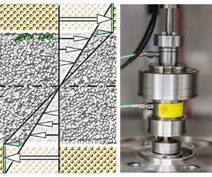
In technical systems the upper and lower surfaces of the adjacent solids are often metals being hardened and usually ground, honed or lapped, showing technical roughness  $k$ with an order of magnitude of $10\, \mathrm {nm}\ \mathrm {to}\ 1\, \mathrm {\mu }\mathrm {m}$, cf. figure 2. In any case, the surfaces in technical applications are far from being atomically smooth (Klocke & König Reference Klocke and König2005). Furthermore, the lubricant is usually mineral oil or synthetic oil. It is therefore a mixture of non-polar molecules with different molecular weights. To positively influence friction by tailor-made fluids, polar molecules, i.e. additives, are added to the lubricant. These molecules adsorb on the metal surface and thus change the dynamic boundary condition, i.e. the slip length $\lambda$ sketched in figures 1 and 5.

Figure 2. Rough metal surfaces after surface treatment (Klocke & König Reference Klocke and König2005). The images were created by means of a scanning electron microscope. For the honed and lapped surfaces, the depths of the groves are of the order of 1  $\mathrm {\mu }$m and 10 nm, respectively. The lapped surface is isotropic, whereas the honed surface is not due to the obvious surface structure. In the experiments described in this paper, all surfaces are lapped.
This work deals with the lubrication flow of Newtonian fluids (constant density  $\varrho$, constant dynamic viscosity $\mu$) in narrow gaps where the mean gap clearance $\bar {h}$ is so small in relation to the slip length $\lambda$ that wall slip becomes relevant. As we will show: for the typical order of magnitude $\lambda /\bar {h}\sim 10^{-2}$ that applies to hydrocarbon lubricated bearings, the wall slip indeed has a non-negligible influence on both the load carrying capacity of the bearing (see figures 13 and 15a) and the energy dissipation in the bearing (see figures 14 and 15b).
Although the theory of hydrodynamic lubrication with Stokes’ no-slip dynamic boundary condition is well developed, there are three open needs or questions regarding Navier's dynamic boundary condition for Newtonian fluids with and without additives in technically relevant flows, cf. § 2: first, there is a particular need for new measurement principles for the robust, automated and reproducible determination of temperature-dependent wall slip on technically relevant rough surfaces. Existing measurement principles, which have been developed and used in nanofluidics in recent years, are either not suitable for the interface between a solid metal surface and a hydrocarbon fluid, or are only suitable to a certain degree for technically relevant systems since the measurement area is too small to average stochastic interface variations. Second, from an epistemological point of view as well as for tailor-made fluids and interfaces, the relation between volume shear and wall slip and its dependence on temperature and molecular structure of hydrocarbon fluids are of interest. Third, in an application, the influence of wall slip on the load-carrying capacity through the force–displacement curve of narrow gaps, i.e. the Sommerfeld number as a function of relative eccentricity in the case of a journal bearing, is of practical interest as well as the friction torque in terms of a sustainability point of view.
The aim of this paper is firstly to discuss the constitutive relationship between shear stress and slip velocity at the liquid–solid boundary from the point of view of rate theory, secondly to measure this constitutive relationship for hydrocarbon lubricants of different molecular structures and thirdly to evaluate the influence of the boundary condition on the energetic and functional characteristics of the gap of a journal bearing.
1.2. Structure of the paper
In order to provide answers to the three open questions, the paper is divided into seven main sections, with this introduction stating the motivation, focus and research questions. § 2 shows that the necessary bridging between the two research fields of nanofluidics and tribology to answer the open questions is not yet sufficiently formed. Wall slip is then discussed from the point of view of rate theory, (§ 3) and in particular from the point of view of the Eyring model (§ 3.1), leading to the conclusion that the activation energy for wall slip  $E_{\lambda }$ in a mixture of non-polar hydrocarbon molecules is expected to be only approximately half of the activation energy for bulk shear, $E_{\lambda }\approx 0.5E_\mu$. This theoretical result will be experimentally validated in the further course of the paper.
For this purpose, § 4 presents a newly developed apparatus called the slip length tribometer (SLT). The SLT is used to simultaneously measure bulk shear and wall slip. This apparatus can be used over a wide and well-controlled temperature range,  $-30\,^\circ \mathrm {C} \le \varTheta = T-273.15\,\mathrm {K} \le 100\,^\circ \mathrm {C}$ with a temperature uncertainty smaller than $0.2\,^\circ \mathrm {C}$.
Model-based estimation, i.e. the Eyring model and the activation energy for wall slip, is experimentally validated, cf. § 5, figure 11 and table 2. The addition of polar molecules to the oil and their influence on slip length is investigated, cf. § 5.3. The results reveal that the addition roughly halves the slip length at room temperature, while the influence on the activation energy is negligible, cf. table 2.
Subsequently, we discuss the impact of wall slip on Sommerfeld's similarity theory of tribology and in particular on the Stribeck curve resulting from this theory (§ 6.3). This is done by employing the SLT measured viscometric constants given by the parameter set [ $\mu _0,E_\mu,\lambda _0,E_{\lambda }$] with $\mu _0=\mu (T_0)$, $\lambda _0=\lambda (T_0)$ at reference temperature $T_0$, see table 2, to predict the load capacity and frictional force of a journal bearing at different temperatures $T$ (see § 6, figures 13–15). For this purpose, the Reynolds equation generalised for wall slip (see Appendix A) is solved both numerically and by means of an asymptotic expansion.
Section 6 also shows that the asymptotic expansion gives a useful approximation of the numerical results, especially for small relative eccentricities and small Sommerfeld numbers. Hence, it provides a rule of thumb to estimate the influence of wall slip on the energy consumption due to tribological contacts. It is shown that the approximate solution is consistent with Petrov's equation (Petrov Reference Petrov1883) generalised for wall slip
To study the impact of wall slip in typical technical systems, § 7 presents two use cases, a typical camshaft journal bearing of a combustion engine and a journal bearing of an industrial compressor. The load-carrying capacity of the bearing as well as the drag force per unit length are compared for the presence and absence of wall slip within the bearing.
Appendix A gives a concise and strict derivation of the generalised Reynolds equation. In Appendix B a strict method to quantify the measurement uncertainty in the context of the SLT is derived. Appendix C finally reports slip lengths and activation energies for the most common lubricants, i.e. the mineral oils VG 46, VG 68. All values are gained with the SLT introduced here.
2. Literature review – wall slip in nanofluidics and tribology
In recent years, research on wall slip has been conducted in the two related research areas of nanofluidics and tribology. As § 2.2 shows, research to date in nanofluidics has focused primarily on the experimental determination of wall slip, often based on the atomic force microscope (AFM), while the focus in tribology (§ 2.3) has been on the theoretical determination of the load-bearing capacity and friction of technical components such as sliders and journal bearings. Previous work on tribology has mostly been of a purely theoretical nature, since experimentally determined input data for wall slip, e.g. in the form of measured slip lengths at technically relevant surfaces, are hardly available. On the one hand, existing experimental work in the field of nanofluidics is of limited value for tribology since stochastic interfacial variations due to interfacial roughness are not averaged and, on the other hand, the available experimental techniques are mostly not suitable for the technically relevant combination of metallic solids and hydrocarbon fluids. The following two subsections show that the two related research areas are not yet sufficiently connected.
An indication of this gap is that, in nanofluidics, the concept of Helmholtz’ slip length is commonly used as an interpretation of Navier's constitutive relation for wall slip, cf. (2.5) in the following subsection on the dynamic boundary condition. Thus, wall slip is interpreted from the perspective of kinematics or even geometry, whereas in tribology wall slip is usually interpreted from the Navier perspective, which relates shear stress to slip velocity or vice versa as in the constitutive relation (2.1), cf. the following subsection. One reason for this discrepancy could be the different length scales considered by the research groups. In nanofluidics, the length scales of interest range from 1 to 10 nm and are given by atomic scales and nano-surface roughness, while in tribology the typical length scales are given by engineering surface roughness and the typical size of a bearing or seal. The order of magnitude of the scales of interest in tribology therefore ranges from 10 nm to 100 mm (or even larger). In order to understand the influence of, for example, friction reducing additives on wall slip (i.e. slip length) but not on shear (i.e. viscosity), it is necessary to consider the scales and methods of nanofluidics holistically with the methods of tribology. This is attempted in this paper.
To provide a foundation for the paper and discussion, this literature review is introduced with a reminder of the boundary conditions at the solid–fluid interface for Newtonian lubricants and the distinction between Newtonian and non-Newtonian material behaviour.
2.1. Boundary conditions at the solid–fluid interface for Newtonian lubricants
As is well known, the kinematic boundary condition at the solid–fluid interface is given by Lagrange's theorem: ‘The interface is always made up of the same fluid particles’. This theorem is expressed in short by the scalar equation D $H/$D
$H/$D $t=0$ with $H=z-h(\boldsymbol x,\,t)=0$ for the upper wall of surface $S_H$ and $H=z=0$ for the lower wall of surface $S$, cf. (A5). Of greater interest than the kinematic boundary condition is the dynamic boundary condition, at least in the context of this paper. It is given by Newton's third law ‘actio est reactio’. This axiom demands the continuity of the stress vector $\boldsymbol{t} = {\rm d}\boldsymbol F/$d $S$ across the wall. The force $\boldsymbol F$ is determined for given $\boldsymbol t$ by integration over the wall surface $S$.
$S$.
If the nonlinear convective terms and the linear transient term on the left-hand side of the equation of motion are negligibly small (for the necessary conditions see Appendix A), which is assumed here, the inductance of the fluid in the gap is negligibly small so that the left side of the equation of motion can be neglected. Hence, the tangential and normal forces  $\boldsymbol D$ and $\boldsymbol N$ on both walls are equal in magnitude and opposite in direction. It is therefore sufficient to consider the forces on the lower wall only. The stress vector at the lower wall $z=0$ with normal vector $\boldsymbol e_z$ is given by $\boldsymbol t=(-p+\tau _{zz}) \boldsymbol e_z+\tau _{iz} \boldsymbol e_i$, $i=1,2$ (we use Einstein's summation convention). With the nonlinear convective terms and the linear transient term being negligible, the normal viscous stress $\tau _{zz}$ is much smaller than the static pressure $p$ and the tangential stress components: $\tau _{zz}/\tau _{iz}\sim \tau _{zz}/p\sim \psi \ll 1$ (Spurk & Aksel Reference Spurk and Aksel2019). The continuity of the normal component $\boldsymbol t\boldsymbol {\cdot } \boldsymbol e_z=-p$ demands the continuity of the static pressure $p$ across the interface, whereas the continuity of the tangential components $\boldsymbol t\boldsymbol {\cdot } \boldsymbol e_i=\tau _{iz}$ requires a constitutive relation, which is the subject of this subsection. This constitutive relation relates the shear stress components $\tau _{iz}$ to the relative slip velocity $w_i=U_i-u_i$ at the wall. Here, $u_i$ is the component of the flow velocity within the gap in the $i=1,2$ direction and $U_i$ is the lateral velocity of the walls, cf. figure 1.
Navier (Reference Navier1822) was the first to formulate a linear constitutive relationship between shear stress and slip velocity. The generalised tensor form of this relationship in Cartesian index notation is as follows:
 \begin{equation} \tau _{iz} = \,f_{ij}w_j, \quad(i,j=1,2). \end{equation}
Here,  $\,f_{ij}$ is the component of wall friction tensor, $\tau _{iz}$ the components of the stress vector tangential to the wall and $w_i=U_i-u_i$ the slip velocity at the wall. Multiplying Navier's slip law by $w_i$ yields the dissipation rate per unit wall surface area $w_i \tau _{iz}=w_i \,f_{ij} w_j$. From this, it follows that $\,f_{ij} = \,f_{ji}$, i.e. the wall friction tensor is symmetric.
The equivalent to Navier's constitutive law for wall slip is Newton's constitutive relation (Newton Reference Newton1687) for viscous friction at the wall for incompressible flow
 \begin{equation} \tau_{iz}= \mu \frac{\partial u_i}{\partial z}, \quad(i=1,2). \end{equation}
 Eliminating  $\tau _{iz}$ from (2.1) and (2.2) yields
 \begin{equation} \mu \frac{\partial u_i}{\partial z} = \,f_{ij}w_j. \end{equation}
 The relation of the slip length tensor  $\lambda _{ij}$ to the wall friction tensor $\,f_{ij}$ is defined by the equation
 \begin{equation} \lambda_{ik}\,f_{kj} := \mu \delta_{ij}. \end{equation}
(here, and in the following, ‘:=’ means ‘is defined to be equal to’ and  $\delta _{ij} = \boldsymbol {e}_i \boldsymbol {\cdot } \boldsymbol {e}_j$ is the Kronecker delta.) Combining (2.3) and (2.4) yields
 \begin{equation} \lambda_{ij}\frac{\partial u_j}{\partial z} = w_i. \end{equation}
Even though this seems to be a kinematic boundary condition, the dynamic character becomes clear.
The technical lubrication gaps being addressed within this paper show isotropic surfaces properties, i.e.  $\,f_{ij}=\,f\delta _{ij}$ and $\lambda _{ij}=\lambda \delta _{ij}$. The slip length $\lambda$ for isotropic surfaces was first introduced by Helmholtz & von Piotrowski (Reference Helmholtz and von Piotrowski1860). Hence, we have $\mu =f\lambda$ for the relation of viscosity $\mu$, friction factor $f$ and slip length $\lambda$. Recent results from molecular dynamics (MD) simulations by Mehrnia & Pelz (Reference Mehrnia and Pelz2021) showed that the apparent viscosity for (non-polar) hydrocarbon alpha-olefin (PAO 6) is shear rate independent up to an apparent shear rate of $\dot {\gamma }_{c} = 10^8\,\mathrm {s}^{-1}$ (see figure 10). Hence, the relaxation time for those typical lubricant with mean molar mass $\bar {M} = 600\, \mathrm {u}$ is approximately 10 ns (inverse of the critical shear rate) at ambient temperature. Furthermore, for the shear rates up to $10^5\,{\rm s}^{-1}$ being realised in the experiments reported in this work and which are relevant in lubrication gaps, the fluid is, in fact, Newtonian with dynamic viscosity $\mu$ and slip length $\lambda$, both being independent of shear rate. This is because apparent wall slip due to shear thinning, i.e. viscoelastic effects, are only expected at shear rates $\dot \gamma \sim \dot \gamma _c$ or larger.
The slip length scales with the effective molecular length  $a$ (Bocquet & Barrat Reference Bocquet and Barrat2007; Lauga, Brenner & Stone Reference Lauga, Brenner and Stone2007). This also results from the generalised Eyring model for wall slip developed in this paper, cf. § 3.1, (3.15). However, the statement $\lambda \sim a$ is only valid for $h\gg a$, which is always assumed in this work. Mehrnia & Pelz (Reference Mehrnia and Pelz2021) considered also the complementary case $h \to a$ by analysing the Couette flow between two plates (gap height $h$, tangential speed $U$) using MD methods. The simulation results show $\lambda \to \infty$ for $h \to a$. In fact, this singularity is easy to see: for $h \to a$ the slip velocity approaches half the relative velocity, $w \to U/2$, for symmetry reasons. As we will show in § 3.1, the adhesion forces between the molecules in the bulk are much larger than the adhesion forces between the non-polar molecules near the wall and the iron atoms of the wall. Therefore, for $h \to a$ the shear rate approaches zero. Equation (2.5) then gives $\lambda \to \infty$ for $h \to a$. We will come back to this when discussing the presented Stribeck curve, figure 15(b), in the asymptotic limit of very large Sommerfeld number and hence small gap height. In this limiting case, the assumption of a constant slip length no longer applies.
2.2. Wall slip in nanofluidics
In nanofluidics, wall slip is usually measured by measuring the slip length tensor  $\lambda _{ij}$ or the relative slip velocity $w_i=U_i-u_i= \lambda _{ij} \, \partial u_j / \partial z |_{z = 0,h}$ between a near-wall fluid particle of absolute velocity $u_i$ and the wall with the absolute velocity $U_i$ (see figure 1). The experiments can be performed either in a controlled laboratory environment (cf. this paper) or ‘in silico’ using MD simulations (Mehrnia & Pelz Reference Mehrnia and Pelz2021). In either case, the determined viscometric constants for both shear, i.e. the dynamic viscosity $\mu$, and wall slip, i.e. the slip length $\lambda$, are both ensemble averaged. Therefore, any method must explicitly or implicitly average over many molecules and many (technical) interface roughness peaks.
2.2.1. Local measurement principles
Over the years, a variety of experimental set-ups and techniques to measure wall slip emerged. See Neto et al. (Reference Neto, Evans, Bonaccurso, Butt and Craig2005), Lauga et al. (Reference Lauga, Brenner and Stone2007), Maali & Bhushan (Reference Maali and Bhushan2012) and Garcia (Reference Garcia2016) just to mention some of the more recent ones. The methods can be divided into optical methods, interfacial resolving dynamic methods and interfacial averaging dynamic methods. Here, dynamic means that it is about force measurements, e.g. by means of the AFM or also wall shear stress integrated over larger surfaces. The last case concerns this paper, in which the dynamic quantity to be measured is torque.
The first two groups of measurement principles can be described as local, while the latter methods can be described as integral. Local methods are common in the research field of nanofluidics, while integral methods are found in the research field of tribology and rheology. Today, the eight most popular local methods applied in nanofluidics are:
(i) Fluorescence recovery after photobleaching, FRAP, (Durliat, Hervet & Léger Reference Durliat, Hervet and Léger1997; Pit, Hervet & Léger Reference Pit, Hervet and Léger1999, Reference Pit, Hervet and Léger2000).
(ii) Total internal reflection-fluorescence recovery after photobleaching, TIR-FRAP (Pit et al. Reference Pit, Hervet and Léger2000).
(iii) Particle image velocimetry, PIV (Restagno et al. Reference Restagno, Crassous, Charlaix, Cottin-Bizonne and Monchanin2002; Joseph & Tabeling Reference Joseph and Tabeling2005).
(iv) Fluorescence correlation spectroscopy, FCS (Joly, Ybert & Bocquet Reference Joly, Ybert and Bocquet2006).
(v) Double-focus fluorescence cross-correlation, DF-FCS (Vinogradova et al. Reference Vinogradova, Koynov, Best and Feuillebois2009).
(vi) Colloidal probe AFM (McBride & Law Reference McBride and Law2010).
(vii) Surface force apparatus, SFA (Horn et al. Reference Horn, Vinogradova, Mackay and Phan-Thien2000).
(viii) Dynamic surface force apparatus, DSFA (Restagno et al. Reference Restagno, Crassous, Charlaix, Cottin-Bizonne and Monchanin2002).
The optical methods (i) to (v) are not well suited for the technical systems we are focused on here. The interfacial resolving dynamic methods, (vi), (vii) and (viii), can be very accurate but are not suited for technically relevant substrates. Although they belong to the same class of experimental techniques, they are technically very different and have various strengths and limitations. The following is an overview of previous research on these methods.
Due to its simplicity and high resolution, of the order of magnitude of  $0.5\,\mathrm {nm}$, the AFM is one of the most widely used methods for measuring wall slip. However, and besides its high resolution capabilities, many researchers have been confronted with significant noise during their measurements (Bonaccurso, Butt & Craig Reference Bonaccurso, Butt and Craig2003; Honig & Ducker Reference Honig and Ducker2007; McBride & Law Reference McBride and Law2010). To overcome the drawback of a noisy measurement signal, Zhu, Attard & Neto (Reference Zhu, Attard and Neto2011) developed an algorithm to reduce the impact of the experimental noise on the derived slip length, resulting in a reported overall systematic measurement uncertainty of only 2 nm (the typically reported measurement uncertainties of the different methods for measuring the slip length are given in table 1).
Table 1. Selection of typically reported measurement uncertainties of the different methods for measuring the slip length ( $^*$ no adequate or transparent uncertainty quantification reported).

The SFA was initially developed to measure drainage forces between two transparent, half-cylindrical mica surfaces (Tabor & Winterton Reference Tabor and Winterton1969; Israelachvili & Adams Reference Israelachvili and Adams1976). Here, the force is obtained by measuring the deflection of a cantilever spring with known stiffness, supporting one of the two mica surfaces. The width, shape and optical index of the gap between the two solids is measured using the fringes of equal chromatic order (FECO) method, cf. Israelachvili et al. (Reference Israelachvili2010). Whereas for example Persson & Mugele (Reference Persson and Mugele2004) moved one surface at a constant speed, the SFA can also be used for oscillatory operation in which the two solids oscillate relative to each other either in the lateral direction (Israelachvili, Mcguiggan & Homla Reference Israelachvili, Mcguiggan and Homla1988) or in the normal direction (Zhu & Granick Reference Zhu and Granick2001; Baudry et al. Reference Baudry, Charlaix, Tonck and Mazuyer2001). For further details on the SFA see the thorough review articles of Neto et al. (Reference Neto, Evans, Bonaccurso, Butt and Craig2005) and Israelachvili et al. (Reference Israelachvili2010).
Zhu & Granick (Reference Zhu and Granick2001) employed a modified SFA with tetradecane liquid confined between solid mica surfaces coated with a methyl-terminated close-packed monolayer of condensed octadecyltriethoxysiloxane. The authors observed a rise in slip length above a critical shear rate and reported slip lengths of the order of magnitude of 1  $\mathrm {\mu }$m. Those high values are presumed to be caused by shear induced nucleation of gas or vapour bubbles on the surfaces. Therefore, they are not typical in terms of slip lengths in general.
The first DSFA was developed by Tonck, Georges & Loubet (Reference Tonck, Georges and Loubet1988). This method allows the measurement of intermolecular forces of a liquid confined between a solid sphere and a solid plane for transient operation. For the DSFA the gap width is measured using a combination of a high resolution interferometric sensor and a capacitive sensor (Restagno et al. Reference Restagno, Crassous, Charlaix, Cottin-Bizonne and Monchanin2002; Cottin-Bizonne et al. Reference Cottin-Bizonne, Steinberger, Cross, Raccurt and Charlaix2008). The wetted area for the used apparatus has an order of magnitude of  $10^3\,\mathrm {\mu }{\rm m}^2$. The fluid is squeezed harmonically by a piezo actor and the inverse of the out of phase force component, i.e. the dissipative viscous force, is plotted vs the measured gap height. By means of linear regression and extrapolation, the slip length is derived.
Due to the deployment of the FECO method, the SFA is limited to transparent surfaces, whereas both the DSFA and the AFM are not limited to transparent substrates. However, the area to be examined (typical radius of the surfaces is of the order of magnitude of 10  $\mathrm {\mu }$m for the DSFA and smaller for the AFM) is too small compared with the area needed to handle technical roughnesses.
Regarding the limitation due to the need for transparent surfaces, FRAP, TIR-FRAP and PIV form a compromise between the SFA and DSFA. These methods require only one transparent substrate, while the other can be opaque. The probed area for FRAP is of the order of  $600\times 600\,\mathrm {\mu }{\rm m}$ (Hénot et al. Reference Hénot, Grzelka, Zhang, Mariot, Antoniuk, Drockenmuller, Léger and Restagno2018).
In conclusion, the limited possibility of measuring technical rough metal surfaces combined with technical lubrication motivated us to think of an alternative measurement principle. The SLT has the advantage of an intrinsic averaging of the slip length over a high measurement area, which leads to the possibility of measuring technically relevant surfaces.
2.2.2. Surface roughness
As mentioned before, technical surfaces are far from being atomically smooth. Therefore, regarding surface roughness in the scope of the paper, a classification of firstly atomic and secondly technical roughness is required. Technically, rough surfaces are the focus of this paper. They are the result of mechanical surface treatment such as grinding, honing or lapping, where the latter is rarely used for cost reasons. When grinding, the technical surface roughness is of the order of 0.2 to 0.8  $\mathrm {\mu }$m. Honed surfaces achieve surface roughness of the order of 0.1 to 0.65 $\mathrm {\mu }$m. A surface roughness of up to 10 nm is achieved by lapping, cf. Gomeringer et al. (Reference Gomeringer, Kilgus, Menges, Oesterle, Rapp, Scholer, Stenzel, Stephan and Wieneke2019). Technical roughnesses are thus in the range 10 nm to 1 $\mathrm {\mu }$m. With the SLT the surfaces are lapped and the arithmetic mean roughness is below 10 nm, cf. § 4.
Atomically rough surfaces show roughness of the order of only 1 to 10 nm. This low roughness often requires a chemical surface treatment, which usually cannot be used in technical systems for environmental reasons (Zhu & Granick Reference Zhu and Granick2002; Bonaccurso et al. Reference Bonaccurso, Butt and Craig2003; Granick, Zhu & Lee Reference Granick, Zhu and Lee2003; Vinogradova & Yakubov Reference Vinogradova and Yakubov2006). The so far investigated surface roughnesses ranged from 0.2 to  $6.0\, \mathrm {nm}$ (Zhu & Granick Reference Zhu and Granick2002), or 0.7 to $12.2\, \mathrm {nm}$ (Bonaccurso et al. Reference Bonaccurso, Butt and Craig2003). The results reported for those surfaces are somewhat contradictory, e.g. increasing or decreasing slip with or without surface roughness (Bonaccurso et al. Reference Bonaccurso, Butt and Craig2003; Granick et al. Reference Granick, Zhu and Lee2003; Zhu & Granick Reference Zhu and Granick2002). A detailed list of research on the influence of nano-scale surface roughness can be found in the review articles by Neto et al. (Reference Neto, Evans, Bonaccurso, Butt and Craig2005), Cao et al. (Reference Cao, Sun, Chen and Guo2009) and Vinogradova & Belyaev (Reference Vinogradova and Belyaev2011).
Regarding the isotropic roughness of technically relevant surfaces being of the order of  $10\, \mathrm {nm}$ to 1 $\mathrm {\mu }$m (see figure 2), surface roughness and also wall slip will be characterised by averaging over a representative and sufficiently large distance or area. Following this paradigm, the measurement of slip length of technically rough surfaces will also be integrally averaged. This requires that the process-specific characteristic length for measuring slip length shall be at least as large as the demanded length or surface area for determining the surface roughness. Otherwise, the measured slip length would not be objective, i.e. independent of the sample and operator.
With regard to the most commonly used techniques, almost all of them measure slip length using small characteristic length scales of the order of 10  $\mathrm {\mu }$m. Therefore, all presented techniques are inadequate for the determination of slip length in technically relevant rough surfaces.
Non-isotropic, i.e. structured, surfaces, which are considered e.g. in the work of Steinberger et al. (Reference Steinberger, Cottin-Bizonne, Kleimann and Charlaix2007), are not the focus of this work.
2.2.3. Temperature dependence of wall slip
In the reviews by Bocquet & Barrat (Reference Bocquet and Barrat2007) and Lauga et al. (Reference Lauga, Brenner and Stone2007), the molecular scale for wall slip was highlighted. Indeed, one task of this paper is to discuss wall slip from a molecular point of view based on rate theory (§ 3.1). This will give us an insight into the relation between the activation energy for slip and shear and will help us to discuss the experimental results.
It appears that Tolstoi (Blake Reference Blake1990) was the first to quantify the effect of surface energies on wall slip at the molecular level. According to Blake (Reference Blake1990), Tolstoi evaluated the relation between molecular layers and surface energies and how it changes near a solid–fluid interface. The Tolstoi model quantifies the slip length as a function of contact angle. According to the Tolstoi model, the slip length would decrease with increasing temperature, which is consistent with the experimental and theoretical results of the present work. Andrienko, Dünweg & Vinogradova (Reference Andrienko, Dünweg and Vinogradova2003) presented an alternative perspective for the dependence of slip length on temperature in terms of a prewetting transition, which is not considered further here.
Pelz & Corneli (Reference Pelz and Corneli2021) based an argument on dimensional analysis combined with an Arrhenius rate equation to relate the activation energy for bulk shear  $E_\mu$ and wall slip $E_{\lambda }$. The authors proposed to derive $E_\mu$ and $E_{\lambda }$ and hence also the activation energy for the friction factor, $E_f=E_\mu -E_{\lambda }$ (cf. § 2.1 for the definition of the friction factor and § 3 for the relation of the different activation energies), by employing an Arrhenius plot for the dynamic viscosity $\mu (T)$ and the slip length $\lambda (T)$.
Alternatively, and independently of arguments based on the Bridgman postulate, in this article we develop the Eyring model for wall slip to make a statement about the relation between the activation energies  $E_\mu$, $E_{\lambda }$, $E_f$, of which, from a phenomenological point of view, only two are independent due to the relationship $E_f=E_\mu -E_{\lambda }$. The Eyring model for wall slip for non-polar molecules leads to $E_{\lambda }\approx 0.5 E_\mu$. Hence, both viscosity and slip length decrease with increasing temperature, consistent with the experimental findings in this paper and the Tolstoi model. This decrease of slip length with increasing temperature is also a result of recent MD simulations by Mehrnia & Pelz (Reference Mehrnia and Pelz2021).
Hénot et al. (Reference Hénot, Grzelka, Zhang, Mariot, Antoniuk, Drockenmuller, Léger and Restagno2018) measured slip length as a function of shear rate for three polymers of different molecular weights utilising a velocimetry technique based on photobleaching. The authors report an increasing slip length with increasing temperature for the non-Newtonian fluid considered. This contradicts the results obtained for Newtonian fluids in this paper. This might be due to the fact that Hénot et al. (Reference Hénot, Grzelka, Zhang, Mariot, Antoniuk, Drockenmuller, Léger and Restagno2018) analysed bulk shear and wall slip of polymer liquids of large molecular weight and not Newtonian fluids of rather small molecular weight, as is the case in this paper. For amorphous polymeric liquids near their glass transition temperature it is well known that the temperature dependence of the bulk viscosity is given by the Williams–Landel–Ferry (WLF) equation and not the Arrhenius equation and it is expected that the temperature dependence of wall slip would be described by a WLF equation as well. Besides this, it was concluded using the relation  $E_f=E_\mu -E_{\lambda }$ that either an increase or a decrease in the slip length with respect to the temperature is to be expected (Pelz & Corneli Reference Pelz and Corneli2021; Hénot et al. Reference Hénot, Grzelka, Zhang, Mariot, Antoniuk, Drockenmuller, Léger and Restagno2018). The experiments presented in this paper, the Eyring model adapted for wall slip (§ 3.1), Tolstoi's model and the MD simulations all predict a decrease in slip length with increasing temperature for hydrocarbon lubricants in the Newtonian regime.
2.2.4. Non-Newtonian fluids
As with the paper of Hénot et al. (Reference Hénot, Grzelka, Zhang, Mariot, Antoniuk, Drockenmuller, Léger and Restagno2018) in terms of the temperature dependence of slip length, most of the research was carried out for non-Newtonian fluids (Yoshimura & Prud'homme Reference Yoshimura and Prud'homme1987; Hatzikiriakos & Dealy Reference Hatzikiriakos and Dealy1991). Hatzikiriakos & Dealy (Reference Hatzikiriakos and Dealy1992) investigated wall slip in a plate–plate tribometer with a non-Newtonian polymer flow to find the relationship between wall slip and shear stress. They stated that wall slip happens above a critical shear stress and it increases with increasing temperature. Andrienko et al. (Reference Andrienko, Dünweg and Vinogradova2003) measured the slip length as a function of temperature for a polymer mixture while the system was under a prewetting transition. Results revealed that the slip length reduces with the temperature rising after the prewetting transition.
2.3. Wall slip in tribology
The focus in tribology is mostly on the theoretical determination of the load capacity and friction of components such as slider and journal bearings under wall slip. In the research area of tribology, wall slip is sometimes regarded with altered shear stress at the wall (Shukla, Kumar & Chandra Reference Shukla, Kumar and Chandra1980; Ma, Wu & Zhou Reference Ma, Wu and Zhou2007; Xie et al. Reference Xie, Rao, Ta-Na, Liu and Chen2016; Xie, Ta & Rao Reference Xie, Ta and Rao2017). Here, Stokes’ no-slip boundary condition is the reference case. Spikes (Reference Spikes2003) used a concept of altered shear stress at the wall to describe a slider bearing with slip occurring at the upper but not the lower wall. By doing this, the author derives a form of Reynolds’ equation in which slip is considered at one of the surfaces. The concept of altered shear stress is not mis-matched with a yield stress of a Bingham medium.
Shukla et al. (Reference Shukla, Kumar and Chandra1980) derived a generalised form of Reynolds’ equation for liquid lubrication regarding an assumed viscosity variation in the gap and considering slip at the bearing surfaces. Cui et al. (Reference Cui, Le, Fillon and Zhang2021) studied the effect of coatings on the behaviour of plain journal bearings, considering wall slip occurring at the interface between oil and substrate, using a slip model introduced by Spikes & Granick (Reference Spikes and Granick2003).
Besides the theoretical work in the field of tribology, there is so far a lack of experimentally determined input data for wall slip, e.g. in the form of measured slip lengths at technically relevant interfaces. In the research area of tribology, integral measurement principles are employed mainly for non-Newtonian fluids.
2.3.1. Integral measurement principles
Cheikh & Koper (Reference Cheikh and Koper2003) employed a capillary to measure wall slip, similar to the historic work of Poiseuille. Since the pressure difference between the inlet and outlet of a capillary expresses the integral of the wall shear stress, it is, in fact, an integral measurement principle as well. Since it is hard to characterise the interface between solid and fluid insight the capillary with regard to surface roughness, a plate–plate topology is preferred in our work.
In tribology (and rheology) co-axial rotating plate–plate or plate–cone devices are common and were used to measure wall slip, especially for non-Newtonian fluids, cf. Henson & Mackay (Reference Henson and Mackay1995), Lee, Choi & Kim (Reference Lee, Choi and Kim2008) and Ming et al. (Reference Ming, Jian, Chunxia, Xiaokang and Lan2011). Henson & Mackay (Reference Henson and Mackay1995) used a plate–plate rheometer to investigate slip of monodisperse polystyrene melts. The discs, each of diameter 7.9 mm, were manufactured from titanium alloy and stainless steel. Lee et al. (Reference Lee, Choi and Kim2008) experimentally studied the effect of geometric parameters of a grooved and holed patterned hydrophobic surface on the liquid slip with a parallel plate geometry in a commercial torsional cone–plate rheometer. It should be noted that the measured slip length using a standard plate–plate or cone–plate rheometer is typically associated with high measurement uncertainty. For instance, Ming et al. (Reference Ming, Jian, Chunxia, Xiaokang and Lan2011) used a plate–plate rheometer to measure the slip length of glycerin solution moving relative to a superhydrophobic surface coated with carbon nanotube forests. From the diagrams shown by Ming et al. (Reference Ming, Jian, Chunxia, Xiaokang and Lan2011), the uncertainty of the slip length measured by them is approximately 2.8  $\mathrm {\mu }$m. This uncertainty is of the same order of magnitude as the gap height. It must therefore be concluded that standard and available plate–plate rheometers are not suitable for measuring wall slip in terms of uncertainty.
Still, the advantage of the integral measurement principle is that averaging over the technical surface roughness is immanent. Therefore, the SLT presented in § 4.1 also uses this averaging, which is inherent in every classical rheometer. The SLT is to be understood as a sophisticated further development of a plate–plate rheometer. The further development offers five specific advantages: firstly, the SLT is robust against kinematic disturbances such as misalignment of the plates, due to the classical fixed and floating bearings of the drive side and the jewel bearing of the driven side. By this means, the two plates on the drive and driven side position themselves naturally parallel to each other due to the levelling effect of the pressure distribution within the gap. Secondly, the SLT is robust with regard to temperature disturbances, e.g. due to dissipation, due to the superimposition of the circumferential Couette flow needed for the measurement of wall slip and bulk shear and the radial Poiseuille flow needed for separating the plates and ensuring a constant temperature. Thirdly, wall slip and bulk shear are measured simultaneously with the SLT offering a convenient means to detect errors. Fourthly, the complete automation of the measurement process allows for a high number of measurement repetitions, making the stochastic measurement uncertainty negligible. Fifth, automation keeps the risk of operator error small. As a result, the formerly mentioned stochastic uncertainties, i.e. noise, are reduced significantly, cf. § 4.5.
2.4. Conclusion of the literature review
As revealed by the literature review, the two disciplines, i.e. nanofluidics and tribology, focus on the same phenomenon from two different directions. Furthermore, it becomes clear that integral measurement principles such as plate–plate rheometers are well suited for measuring wall slip on technically rough surfaces. However, for relevant rough surfaces, there is no measurement device for objectively determining the slip length at different temperatures available at the moment. In fact, Cao et al. (Reference Cao, Sun, Chen and Guo2009) stated that there is a general need to develop new experimental techniques to overcome the uncertainty when measuring nano-scale effects near liquid–solid surfaces. To comply with this request, the SLT is introduced in § 4. Before the detailed description of the SLT, however, we discuss wall slip from the point of view of rate theory. This leads to the conclusion that the activation energy for wall slip  $E_{\lambda }$ in a mixture of non-polar hydrocarbon molecules is expected to be only approximately half of the activation energy for bulk shear, $E_{\lambda }\approx 0.5E_\mu$. This is, in fact, validated by our experiments, cf. § 5.
3. Generalised Eyring model for wall slip and activation energy for shear and slip
As shear takes place in the bulk and slip at the wall, the starting points are the two phenomenological constitutive relations, first Newton's law for the shearing motion of two fluid layers and second Navier's law for slip of a fluid layer relative to a wall. For a Newtonian flow, Newton (Reference Newton1687) described the response of a fluid to shear stress  $\tau$ in the constitutive law
 \begin{equation} \tau = \mu(T)\dot{\gamma}. \end{equation}
 The response is a shear rate  $\dot {\gamma }$ that is, for a Newtonian fluid, proportional to the shear stress $\tau$. The shear rate is a measure of the relative velocity $\Delta u = a\dot {\gamma }$ of two adjacent fluid layers separated by the normal distance $a$. The viscometric function, the dynamic viscosity $\mu (T)$, is already needed on dimensional grounds. The viscosity is a function of the molecules’ activation, the inner energy measured by the absolute temperature $T$. On statistical grounds and heuristic arguments, Eyring derived the Arrhenius function, $\mu (T)\propto \exp (E_\mu /\mathcal {R}\,T)$, arguing that the activation energy for shear $E_\mu$ is the difference of two Gibbs free energies in the context of transition state theory (Bird, Stewart & Lightfoot Reference Bird, Stewart and Lightfoot2007); $\mathcal {R}$ is the universal gas constant.
The second phenomenological constitutive relation is Navier's slip law (Navier Reference Navier1822), see § 2.1
 \begin{equation} \tau = f(T)w. \end{equation}
 The response of the fluid near the wall to a shear stress  $\tau$ is a slip velocity $w$. The viscometric function is the friction factor $f(T)$. Helmholtz & von Piotrowski (Reference Helmholtz and von Piotrowski1860) introduced the slip length
 \begin{equation} \lambda(T) = \frac{\mu(T)}{f(T)}. \end{equation}
 It is the task of this section to derive  $f(T)\propto \exp (E_f/\mathcal {R}T)$ and $\lambda (T)\propto \exp (E_{\lambda }/\mathcal {R}T)$ and discuss the relation of activation energy for shear $E_\mu$ and slip $E_f$, $E_{\lambda }$. Due to (3.3), the activation energies are related by
 \begin{equation} E_{\lambda} = E_\mu -E_f\quad \mathrm{or}\quad \frac{E_{\lambda}}{E_\mu} + \frac{E_f}{E_\mu}=1. \end{equation}
Here,  $E_\mu$ is usually derived by viscosity measurements at different temperatures, or it may be estimated by the evaporation temperature $T_v$ using the relation
 \begin{equation} E_\mu\approx 3.8\, \mathcal{R} T_v \end{equation}
(Bird et al. Reference Bird, Stewart and Lightfoot2007).
The results of the following section are threefold:
(i) The slip length derives the concise result $\lambda (T) = a \exp (E_{\lambda } / \mathcal {R}T)$.
(ii) The slip length scales with the distance between two molecule layers
$a$, i.e. the effective molecular size.(iii) For a weak interaction of the molecules with the solid wall, we derive
$E_{\lambda }\approx 0.5 \, E_\mu$. This will be validated by the experimental results shown in § 5 (see figure 11 and table 2).


Table 2. The table gives the quadruple  $[\mu (T_0),E_\mu,\lambda (T_0 ),E_{\lambda }]$ for each of the four investigated oils measured by the SLT. The reference temperature is $T_0 = 313.15\,\mathrm {K}$, $\varTheta _0 = 40 \, ^\circ \mathrm {C}$. In addition, for verification purposes the dynamic viscosity $\mu _{ref}(T_0)$ as well as the activation energy for bulk shear $E_{\mu,{ref}}$ of the four oils obtained by a capillary rheometer is given.

3.1. Eyring model for bulk shear and wall slip
Recapturing bulk shear, based on well-known literature, e.g. Bird et al. (Reference Bird, Stewart and Lightfoot2007), we discuss the similarity and difference of shear and slip. Eyring (Reference Eyring1935) developed an understanding of viscous friction based on the Eyring rate equation
 \begin{equation} k=\frac{k_B T}{\hslash} \exp\left(-\frac{E}{\mathcal{R}T}\right). \end{equation}
The introduced rate may be seen as a generalisation (Pollak & Talkner Reference Pollak and Talkner2005) of the Arrhenius (Reference Arrhenius1889) rate
 \begin{equation} k=A \exp\left(-\frac{E}{\mathcal{R}T}\right). \end{equation}
Often only relative rates are of interest. Therefore, the prefactor is often eliminated (Pollak & Talkner Reference Pollak and Talkner2005).
In the rate equation (3.6),  $k_B$ is the Boltzmann and $\hslash$ the Planck constant, whereas $E$ is the molar free energy of activation. This is the Gibbs free energy at a transition state minus the minimal Gibbs free energy along the reaction path. In the context of the Arrhenius equation, this energy is often called the activation energy, a term we prefer due to its widespread usage, although it is somewhat less precise.
Figure 3(a) shows the Eyring model of bulk shear. The effective molecular size is given by the distance  $a$ of the cages and holes. The heuristic model reads as follows: a molecule is usually trapped in a cage. By thermal activation, it may escape through a bottleneck into a hole at a distance $a$. The bottleneck is due to the adjacent molecules in the upper or lower molecular layer. The jumps take place with a rate $k$ being different for shear and slip. The shear stress $\tau$ reasons the non-equilibrium and hence asymmetry of the process with regard to forward (index $+$) and backward (index $-$) jumps. The kinematic response is the velocity difference between two molecule layers. It is the effective molecular size $a$ multiplied with the net rate, i.e.
 \begin{equation} \Delta u = a\dot{\gamma}=ak_\mu=a(k_{\mu+}-k_{\mu-}). \end{equation}
Figure 3. (a) Eyring model for bulk shear. The sketch (a) is adapted from the figure shown in Bird et al. (Reference Bird, Stewart and Lightfoot2007); (b) wall slip near a solid wall.
The energy equation formulated for one mole of molecules (the number of molecules is given by the Avogadro constant  $N_A$) occupying the molar volume $V_m$ moving forward or backward reads
 \begin{equation} E_{\mu\pm} = E_\mu \mp \tfrac{1}{2}\tau V_m. \end{equation}
Here,  $E_\mu$ is the activation energy for the fluid at rest. Hence, the constitutive relation between shear rate and shear stress is derived in the Eyring model as
 \begin{equation} \dot{\gamma}=\frac{\Delta u}{a}=\tau \frac{V_m}{\hslash N_A}\exp\left(-\frac{E_\mu}{\mathcal{R}T}\right) + O\left(\frac{\tau V_m}{\mathcal{R}T}\right)^3. \end{equation}
For  $\tau V_m \ll \mathcal {R}T$ the dynamic viscosity is given by
 \begin{equation} \mu(T)=\frac{\tau}{\dot{\gamma}}=\frac{\hslash N_A}{V_m}\exp\left(\frac{E_\mu}{\mathcal{R}T}\right). \end{equation}
For practical application, (3.9) is used in the equivalent form, i.e. the time–temperature shift factor
 \begin{equation} a_\mu(T,T_0):=\frac{\mu(T)}{\mu(T_0)}=\exp\left[\frac{E_\mu}{\mathcal{R}}\left(\frac{1}{T}-\frac{1}{T_0}\right)\right]. \end{equation}
As was mentioned earlier, due to the relative formulation the prefactor  $\hslash N_A/V_m$ is eliminated. Here, $\mu _0=\mu (T_0)$ is the dynamic viscosity at a reference temperature. The activation energy is determined by an Arrhenius graph, i.e. a semilogarithmic plot of the viscosity ratio vs the inverse temperature (see figure 11).
With the schematic shown in figure 3(b) the transfer to wall slip is straightforward but new. From the heuristic model, it is made evident by replacing  $\Delta u$ by the slip velocity $w$. Besides this, the interpretation and the complete derivation remains unchanged, yielding
 \begin{equation} \frac{w}{a}=\tau\frac{V_m}{\hslash N_A}\exp\left(-\frac{E_f}{\mathcal{R}T}\right) + O\left(\frac{\tau V_m}{\mathcal{R}T}\right)^3. \end{equation}
For  $\tau V_m \ll \mathcal {R}T$ the friction factor is derived as
 \begin{equation} f(T)=\frac{\tau}{w}=\frac{1}{a}\frac{\hslash N_A}{V_m}\exp\left(\frac{E_f}{\mathcal{R}T}\right). \end{equation}
 The result is more concise and easy to remember using the slip length. Since the slip length is a relative quantity, i.e. the ratio of two dynamic viscometric functions, the prefactor  $\hslash N_A/V_m$ is eliminated, yielding with (3.3),
 \begin{equation} \lambda(T) = a \exp\left(\frac{E_\mu -E_f}{\mathcal{R}T}\right) = a\exp\left(\frac{E_{\lambda}}{\mathcal{R}T}\right). \end{equation}
 From this result and the model, we draw several conclusions: first, the slip length scales with the effective molecular length  $a$. A result that is evident on dimensional grounds and in accordance with Bocquet & Barrat (Reference Bocquet and Barrat2007) and Lauga et al. (Reference Lauga, Brenner and Stone2007). Second, comparing the two schematic illustrations in figure 3(a,b) it is evident that the two bottlenecks for shear and slip differ, since for the latter there are only a few or even no molecules trapped in the near-wall holes. For an oil–metal interface, this is likely the case for a mixture of non-polar hydrocarbon molecules typically used in technical applications. We expect $E_f$ to be smaller than $E_\mu$. In fact, $E_f\approx 0.5 E_\mu$ should hold for non-polar molecules, since only half of the molecules contribute to the bottleneck. Again, for experiments and applications typically the relative formulation
 \begin{equation} a_{\lambda}(T,T_0) := \frac{\lambda(T)}{\lambda(T_0)}=\exp\left[\frac{E_{\lambda}}{\mathcal{R}}\left(\frac{1}{T}-\frac{1}{T_0}\right)\right], \end{equation}
with  $\lambda _0 = \lambda (T_0)$ is used being the slip length at a reference temperature. The activation energy $E_{\lambda }$ may be determined again by plotting the logarithm of the time–temperature shift factor for wall slip vs $1/T$ (see figure 11). With $E_f \approx E_\lambda\approx 0.5 E_\mu$ and (3.5) a first guess for the activation energy of wall slip would be
 \begin{equation} E_{\lambda} \approx 1.9\, \mathcal{R} T_v , \end{equation}
for molecules with no affinity to the wall.
The result  $E_{\lambda }=E_\mu -E_f\approx 0.5 \, E_\mu$ is indeed confirmed by the experimental results for the non-polar hydrocarbons presented in § 5 (see figure 11 and table 2). We will further show how the Eyring model for wall slip proposed here serves to determine the effective molecular size $a$ as well as the molar volume $V_m$ based on the SLT presented in the following section.
4. Slip length tribometer
In order to provide adequate viscometric functions  $\lambda (T)$ and $\mu (T)$ at different absolute temperatures $T$ (relative temperature $\varTheta =T-273.15$ K), the present section presents and discusses a newly developed integral measurement apparatus, the SLT. Here, we use Helmholtz’ concept of slip length, which is consistent with Navier's constitutive relation between wall shear stress and relative slip velocity. Our preference originates from the fact that the slip length can be graphically interpreted as an effective increase in gap clearance, cf. figure 5. Subsequently and similar to the concept of the DSFA, the slip length is obtained via extrapolation. In addition, the SLT allows the synchronous measurement of wall slip and bulk shear in a technical relevant temperature range for relevant rough surfaces. Therefore, the introduced SLT is reliable and unique for measuring the temperature-dependent slip length of atomically smooth, atomically rough as well as of technically rough surfaces. Being an integral measurement method makes it valuable for gaining insight into technically relevant fluid–solid interfaces.
4.1. Measurement principle of the SLT
To overcome the drawbacks and end up with a robust apparatus that is applicable for quantifying viscosity and slip length simultaneously for technical lubrication gaps at relevant temperatures, the SLT was designed, cf. figure 4.

Figure 4. (a) Schematic sketch of the SLT; disk radius  $R = 32\, \mathrm {mm}$). The temperature is controlled by tempering the rheometer as well as the fluid in a temperature test chamber. The volume flow $Q$ allows a constant temperature within the narrow gap. (b) Photograph of the SLT.
Consisting of two circular plates, the SLT uses the fact that for a Couette flow the true gap height  $h$ of a technical lubrication gap is effectively increased by twice the slip length (see figure 5a). To determine the slip length, the real gap height between the upper rotating disk and the lower stationary one as well as the transmitted frictional torque $M$ by the flow from the upper to the lower plate is measured. By plotting the inverse torque $M^{-1}$ vs the measured true gap height $h$, originating at the lower disk surface, all measurement points $x_i = h_i,y_i=M_i^{-1}$, with $i$ being the index of the measurement point, fall on a straight line $y=a\kern0.7pt x+b$. Considering the polar second moment of area $I_p:=\int _S r^2\,\mathrm {d}S$ of the disks, the slip length $\lambda$ is derived by a linear regression and extrapolation (see figure 5b)
 \begin{equation} M^{{-}1}=\frac{h+2\lambda}{\mu\varOmega I_p}. \end{equation}
Figure 5. (a) Effectively increased lubrication gap by the slip lengths. (b) Sketch of the measurement principle of the SLT for measuring the temperature-dependent slip length and bulk viscosity. The uncertainty quantification for the SLT is given in Appendix B.
In order to manage and minimise the measurement uncertainty, the rheometer was designed as follows.
The chosen motion is rotational with a constant rotational speed  $\varOmega = 2{\rm \pi} n/60$. This is because steady rotating motions can be realised much more precisely than a translation motion by using proven design elements such as bearings, springs and electrical drives. Hence, the apparatus is designed out of two plane circular discs of radius $R=32\, \mathrm {mm}$ each. Both disks are made of an edge hardened stainless steel (steel type 1.8519). The surface is treated by state-of-the-art lapping techniques (see figure 2) resulting in a disk planarity of $15\, \mathrm {nm}$ and an isotropic surface with arithmetic mean roughness below $10\, \mathrm {nm}$.
The presented set-up has a characteristic length of  $2R = 64\,\mathrm {mm}$. This is much larger than the demanded length for determining the surface roughness, i.e. a measurement length of $80\,\mathrm {\mu }{\rm m}$ for a surface roughness of $10\, \mathrm {nm}$. The wetted area is of the order $3\times 10^3\, \mathrm {mm}^2$ and thus six orders of magnitude larger than the wetted area of known apparatus for measuring wall slip. This enables an in situ or built-in reduction of uncertainty.
For the SLT, the lower disc is resting, supported by a jewel needle bearing, allowing a cardanic levelling. The upper disc is rotating and shows a flexible support in the axial direction. The gap height  $h$ is controlled by the fluid pressure $p$ at the fluid inlet through a central bore. For the control loop, the gap height is measured by two capacitive distance sensors integrated into the stationary circular disk at different radii $R_1 = 15\,\mathrm {mm}$ and $R_1 = 25\,\mathrm {mm}$ with an angular offset of $90\,^\circ$. With a measurement range of $400\, \mathrm {\mu }\mathrm {m}$ and a resolution of $4\, \mathrm {nm}$, both sensors are used to measure the gap height $h$ and as a control device of the correct alignment of the disks. The thermal expansion of $100\, \mathrm {nm}\,^{\circ }{\rm C}^{-1}$ limits the uncertainty to $\delta x < 60 \, \mathrm {nm}$.
4.2. The in situ calibration of the SLT
Since the electric capacity of the gap depends on the lubricant as well as on the temperature, the capacitive sensors need to be calibrated in situ. Within the SLT the sensors are used for absolute displacement measurement of fluids with different relative permittivity at varying temperature. Therefore, the permittivity of the fluid has to be known as well as the absolute position of the sensor to the gap surface. The temperature-dependent calibration of the capacitive distance sensors is realised by an interferometric thickness measurement (see figure 6a).

Figure 6. (a) Absolute calibration set-up for the capacitive distance sensors by means of the wavelength of light; (b) temperature-dependent calibration curves of the integrated capacitive sensors.
For this, a high-precision Precitec CHRocodile SE in combination with an interferometric probe IF 40 + Soft is used. The interferometric probe is supplied by a halogen white light source through a fibre optics and a fibre coupler. The Precitec CHRocodile SE in combination with the interferometric probe IF 40 + Soft is capable of measuring up to two transparent layers with a systematic uncertainty of  $13.2\,\mathrm {nm}$. The systematic measurement uncertainty of the voltage measurement can be neglected compared with the other uncertainties. This is because the analogue-to-digital conversion is performed with a 24-bit converter so that the voltage is converted with an accuracy of $596 \times 10^{-9}\,\mathrm {V}$. Converted to the measurement range of the sensor, this corresponds to a resolution of $0.024\,\mathrm {nm}\,\mathrm {bit}^{-1}$.
4.3. Strategies to minimise stochastic and systematic uncertainty – assuming a worst-case uncertainty propagation
In the context of the paper, we have used the terms systematic and stochastic uncertainty several times so far. The former used to be called bias error, the latter random error (Abernethy, Benedict & Dowdell Reference Abernethy, Benedict and Dowdell1985). Today, the terms systematic and stochastic uncertainty are common (Joint Committee for Guides in Metrology 2008; Kamke Reference Kamke2010; Bailer-Jones Reference Bailer-Jones2017; Pelz et al. Reference Pelz, Groche, Pfetsch and Schaeffner2021). The term systematic uncertainty is used for all reproducible measurement errors that can be attributed to a measurement set-up with individually selected sensors and corresponding calibration curves, whereas the term stochastic uncertainty is used for all data that show a probability distribution when performing different measurement runs with the particular measurement set-up.
Within this paper, our strategy to minimise stochastic uncertainty is automation of the measurement system, which offers the possibility to conduct a large number of measurement runs leading to a low variance, cf. § 4.5. Measurements with low variance are usually called precise (Bailer-Jones Reference Bailer-Jones2017).
For systematic uncertainty, the primary means of minimisation is (i) calibration of the sensors, (ii) robust design and operation of the apparatus, i.e. minimal sensitivity to disturbances, and (iii) accurate fabrication and assembling of the parts. These three points were carefully taken into account during the development of the SLT. Measurements with small systematic uncertainty and hence a small bias are called accurate (Bailer-Jones Reference Bailer-Jones2017).
In terms of accuracy, the measurement of the gap width is crucial. Hence, as mentioned, we calibrate the capacitive distance sensors in situ by an interferometric measurement method. But this calibration sensor also shows stochastic and systematic uncertainties that shall be taken into account. Usually, only a constant overall uncertainty within an incertitude interval of say a sensor is given and not the uncertainty distribution function of the sensor. Hence, when it comes to uncertainty quantification, there is the question of how to propagate such a combined systematic and stochastic uncertainty jointly with other stochastic uncertainty using Gaussian uncertainty propagation, cf. Pelz et al. (Reference Pelz, Groche, Pfetsch and Schaeffner2021).
Our answer to the raised question is a worst-case uncertainty quantification according to the procedure suggested by Joint Committee for Guides in Metrology (2008) and Kamke (Reference Kamke2010) resulting in an upper bound for the measurement uncertainties of the slip length and all other derived measures such as the activation energies for wall slip and bulk shear.
In this quantification method, the uncertainty distribution of a sensor is assumed to be uniform between the given uncertainty bounds. This uniform distribution is mapped to a representing Gaussian, i.e. normal, distribution by multiplying the given uncertainty by  $1/\sqrt {3}$ to gain the standard deviation of the representing Gaussian distribution (Joint Committee for Guides in Metrology 2008; Kamke Reference Kamke2010). We use this worst-case approach to methodically account for the uncertainty interval of both the torque sensor and the interferometric sensor in the Gaussian uncertainty propagation method, cf. (B12).
With the interferometric measurement, the thickness of the lubricating film between the upper and lower disks and the voltage signal of the capacitive distance sensor are measured simultaneously. To measure film thicknesses with the interferometric sensor, optical accessibility is required and the refractive indices at the interface of optical accessibility and test liquid must differ sufficiently. Optical accessibility is achieved by replacing the upper rotating disk with an optically continuous flat glass with a planarity of  $\pm 15\, \mathrm {nm}$. The thickness measurement is based on the superposition of the light reflected at both interfaces. If the refractive index of the film is known, the thickness can be determined from the spectrum of the reflected light, i.e. the refractive index. The refractive index of the glass is 1.41 and for the test liquids ranges from 1.41 to 1.48, and these were measured outside the laboratory at a commercial provider. For the liquids, a multi-wavelength refractometer Abbemat MW was used. The uncertainty of the measured refractive index of the liquids is reported as $\pm 4 \times 10^{-5}$ at a wavelength of $589.3 \, \mathrm {nm}$ at $20 \, ^\circ \mathrm {C}$. The refractive indices were measured at eight different wavelengths, ranging from $436.4$ to $657.2 \, \mathrm {nm}$ and two temperatures $12.5\,^\circ \mathrm {C}$ and $60.2\,^\circ \mathrm {C}$. The relative deviation of the measured values at $12.5\,^\circ \mathrm {C}$ and $60.2\,^\circ \mathrm {C}$ is approximately $1\,\%$.
In order to achieve a sufficiently large difference in the refractive indices between the interface and the test liquid as well as electrical conductivity at the same time, the glass is coated with optically continuous and electrically conductive indium tin oxide with a refractive index of 1.80. With the absolute calibration method presented, the capacitive distance sensors are used for different liquids at different temperatures. To reiterate, the calibration is absolute with the wavelength of light. From the above considerations, the systematic uncertainty of the distance measurement is determined to  $\delta x = 60\,\mathrm {nm}$.
4.4. Control and evaluation of the temperature-related uncertainty
To minimise the uncertainty regarding ambient conditions, the SLT is placed inside a temperature test chamber. Within the chamber, the temperature is controlled over a temperature range from  $-30$ to $100\, ^{\circ }\mathrm {C}$ with an uncertainty of max. $\pm 0.1 ^{\circ }\mathrm {C}$. To guarantee a uniformly heated test bench, the SLT is tempered for several hours before starting the measurements. The variation of the temperature inside the temperature test chamber allows a temperature-dependent calibration as well as temperature-dependent measurement of the slip length.
The pressure difference  $p$ between the pressure at the fluid inlet (see figure 4) and the ambient pressure at the gap outlet forces a radial Poisson flow of volume flow $Q$ superimposed on the circumferential Couette flow. Both flows are independent of each other due to the linearity of the equation of motion and the linearity of the boundary condition at the solid–liquid interface (see § 2.1 and Appendix A).
On the one hand, the gap clearance  $h$ is closed loop controlled via the pressure difference $p$. On the other hand, the pressure difference $p$ enables the radial Poisson flow of the volume flow $Q$, which is necessary and desired for the constant temperature maintenance of the fluid in the narrow gap. In fact, this works remarkably well. With the SLT the fluid viscosity can be used as an indirect temperature sensor. Corneli (Reference Corneli2019) showed that the temperature in the gap fluctuates by a maximum of only $\pm 0.2\, ^\circ \mathrm {C}$. This indirect estimate of the temperature-related uncertainty was confirmed by a simulation of the temperature field in the gap taking into account dissipation and convective as well as diffusive heat conduction.
For a given relative velocity  $\varOmega r$ (radius $0< r\leq R$, rotational speed $\varOmega$) the shear stress is inversely proportional to gap clearance: $\tau ^{-1}=(h+2\lambda )/(\mu \varOmega r)$. The transmitted frictional torque $M = 2{\rm \pi} \,\int _{0}^{R}\tau r\, \mathrm {d}r$ is measured using a piezoelectric torque sensor with a measurement range of $\pm 1\, \mathrm {N\ m}$ and a uniform distributed uncertainty of $\pm 0.7 \times 10^{-3}\,\mathrm {N\ m}$. The uncertainty of the inverse torque is maximum at minimum transmitted frictional torque. Thus, at a minimum measured torque of $0.1\,\mathrm {N\,m}$, the normal distributed uncertainty of the inverse frictional torque is determined to $\delta y = \delta M^{-1} < 0.04\, (\mathrm {N\ m})^{-1}$. During the parameter studies, a reproducibility of $3\times 10^{-3}\, \mathrm {N\ m}$ was determined.
4.5. Minimising stochastic uncertainty through number of data points
An adequate and transparent uncertainty quantification is important (Pelz et al. Reference Pelz, Groche, Pfetsch and Schaeffner2021). Therefore, the discussion and presentation of the regression method and Gaussian error propagation used for the SLT are presented in Appendix B.
The total measurement uncertainty of slip length is determined in two steps: (i) first the stochastic and the systematic measurement uncertainty are considered determining the uncertainty of the intercept  $\delta a$ with the abscissa and slope $\delta b$ (see figure 6); (ii) second, the calculated uncertainty of the intercept $\delta a$ and slope $\delta b$ is used in a Gaussian uncertainty propagation giving the uncertainty of the slip length measurement $\delta \lambda$. For the measurement presented in figure 9 the slip length uncertainty is $\delta \lambda = 39\,\mathrm {nm}$. Considering a $95\,\%$ confidence interval, the slip length is measured with an uncertainty of $\delta \lambda _{95\,\%} = \pm 76\,\mathrm {nm}$. Due to the fact that all measurements are carried out using the same equipment, i.e. sensors, data acquisition systems, calibration devices, the systematic uncertainty of the measurements is the same for all measurements. However, the stochastic uncertainty differs from measurement to measurement. Due to the large number of data points for each measurement, cf. § 5, the stochastic uncertainty is reduced to such an extent that it becomes negligible. Nevertheless, it is included in the uncertainty quantification by means of the empirical variance, cf. (B10).
5. Viscometric and molecular parameters derived from SLT slip measurements and Eyring model
In the following, the results of the conducted experiments are provided and consequently molecular quantities are derived using the generalised Eyring model for non-polar molecules. First, the temperature of the fluid is varied, leading to the mentioned Arrhenius plot. Secondly, the influence of molecular mass on slip length is observed by experimentally varying the molecular mass, structure and polarity of a hydrocarbon liquid. The influence of polarity on the molecular distribution in the gap is shown schematically in the figure 7.

Figure 7. Bulk shear and wall slip of (a) non-polar molecules moving relative to a metal wall; (b) polar molecules adsorbed to a metal wall reduce wall slip.
Overall, the activation energy for bulk shear and wall slip shall both depend on the van der Waals forces and hence on two major factors: first on the molecule's length, i.e. the geometric mean average of the molar mass  $\bar {M}$; second on the polarity of the molecules.
To shed some light on this, the molecular structure from the unsaturated hydrocarbon alpha-olefin is varied, being a mixture of three main fractions (see figure 8) to two saturated hydrocarbons, i.e. mineral oils of mean molar mass  $\bar {M} = 666\, \mathrm {u}$ (ISO VG 46) and $806\, \mathrm {u}$ (ISO VG 68). Finally, a small fraction of long chained molecules with polar end groups (Viscosity Index Improver, VI) is added to the mineral oil (ISO VG 46). Adding a small fraction of long chained molecules changes the viscosity as well as the activation energy for bulk shearing. The fraction of the added molecules is selected in a manner such that the viscosity of the blended mineral oil (ISO VG 46+VI) at $40\,^\circ \mathrm {C}$ corresponds to the viscosity of the mineral oil ISO VG 68 at the same temperature. To ensure that no residues of the previous oil affect the molecular structure of the subsequent oil, the rheometer is completely dis- and reassembled after each experiment, cleaning all parts with acetone and a special cleaning liquid.

Figure 8. Area normalised molar mass distribution for the alpha-olefin (PAO 6), the mineral oils (ISO VG 46, ISO VG 68) as well as for the mineral oil blended with a small fraction of polar lubricant additive (ISO VG 46 + VI).
5.1. SLT measurement of a synthetic non-polar hydrocarbon lubricant (PAO 6) moving relative to a metal wall
Figure 9 shows the measurement results of the temperature variation on the slip length for a hydrocarbon alpha-olefin (PAO 6). The temperature was varied in a range of  ${12.5 \, ^\circ \mathrm {C} \leq \varTheta \leq 60.0 \, ^\circ \mathrm {C}}$. Due to the very low stochastic uncertainty, the error bars disappear behind the markers.

Figure 9. Slip length measurements for a synthetic hydrocarbon alpha-olefin (PAO 6). The temperature was varied in a range of  $12.5\,^\circ \mathrm {C} \leq \varTheta \leq 60.0\,^\circ \mathrm {C}$. The measurement uncertainty of gap height and torque are so small that the uncertainty intervals are hidden behind the markers. Nevertheless, the existing uncertainties are taken into account in the uncertainty propagation according to Appendix B to determine the measurement uncertainty of the slip length.
To reduce the stochastic uncertainty of the slip length measurement,  $20$ to $40$ measurement series are performed in each measurement run. Each measurement series consists of $15$ to $20$ measurement points. Each measurement point is averaged over $70\,000$ individual measurements in a measurement interval of 10 s. Each linear regression is supported by $300$ to $800$ measurement points for one single slip length measurement only. The evaluation of the linear regression is based on the measurement points of all measurement series, using a robust bisquare weighted fit to exclude possible outliners (The MathWorks, Inc. 2021). By using the bisquare fitting algorithm, a specific weight is assigned to each measurement point. Here, outliners, i.e. data points far from the linear regression curve, are weighted less than data points close to the curve. Therefore, their impact on the measured slip length and viscosity is reduced. The measurement results in figure 9 show that, with an increase in temperature, the slopes of the graphs increase and the intersection with the abscissa, i.e. twice the slip length $2\lambda$, moves to the origin of the ordinate. This is reasonable because an increased temperature results in a decreased dynamic viscosity of the alpha-olephin, leading to an increased slope of the graph. Furthermore, the increased temperature results in a decreasing wall slip, i.e. slip length at the fluid–metal interface. The measured mean slip length for the synthetic hydrocarbon alpha-olefin (PAO 6) at $40\,^\circ \mathrm {C}$ is $\lambda = 464\, \mathrm {nm}$, whereas the slip length reduces to $\lambda = 348\, \mathrm {nm}$ at a temperature of $60\,^\circ \mathrm {C}$.
In addition, the linear behaviour of the inverse frictional torque  $M^{-1}$ is revealed. Thus, the assumption of linear velocity profiles within the lubrication gap is valid. The coefficient of determination $r^2$ for (4.1) is above $0.999$. Based on this linearity of the inverse frictional torque, the earlier mentioned shear rate independence of the slip length is asserted: all measurements plotted in figure 9 show the same slip length, even though the shear rate varies from ${2 \times 10^3\,\mathrm {s}^{-1}\ \mathrm {to}\ 2\times 10^5\,\mathrm {s}^{-1}}$ over the plate radius. This is consistent with recent results obtained by Mehrnia & Pelz (Reference Mehrnia and Pelz2021) who showed that the apparent viscosity for hydrocarbon alpha-olefin (PAO 6) is shear rate independent up to a apparent shear rate of $\dot {\gamma }_{c} = 10^8\,\mathrm {s}^{-1}$ (see figure 10).

Figure 10. Molecular dynamic simulation (marker) of the apparent dynamic viscosity  $\mu _{{app}} = \tau /\dot {\gamma }_{{app}}$ at different apparent shear rates $\dot {\gamma }_{{app}}=U/h$ for a hydrocarbon alpha-olefin (PAO 6) at $T = 293\,{\rm K}$, cf. Mehrnia & Pelz (Reference Mehrnia and Pelz2021).
The temperature-dependent slip length measurements are now used to calculate the activation energy for bulk shear and wall slip (see § 3.1). For this purpose, in addition to the slip length, the dynamic viscosity is determined from the measurement data of the SLT. For reference purposes, the dynamic viscosity of is also determined using a Lauda iVisc capillary rheometer.
Figure 11 shows the Arrhenius plot for the synthetic hydrocarbon alpha-olefin (PAO 6). The time–temperature shift factors for bulk shear  $a_\mu (T,T_0)$ and wall slip $a_{\lambda }(T,T_0)$ are plotted vs the inverse absolute temperature $T$. The solid lines represent the fit through the measurement data obtained by the SLT, whereas the dashed line and diamond markers represent the fit related to the data obtained by the reference capillary rheometer. Due to the high accuracy of the measurement, the error bars for the viscosity disappear behind the markers. Examining the figure more closely, the time–temperature shift factors for bulk shear and wall slip show the former mentioned dependencies. In addition, the comparison between the time–temperature shift factors for bulk shear obtained by the SLT and the reference capillary rheometer shows a very good agreement. This supports the quality of the newly developed SLT. As predicted by the Eyring model, both relations, (3.12) and (3.16) are observed. The activation energy for bulk shear of the alpha-olefin obtained by the SLT is $E_\mu = (36.4 \pm 1.11) \, \mathrm {kJ}\, \mathrm {mol}^{-1}$. The experiments indicate an activation energy of $E_{\lambda } = (12.8 \pm 4.8)\, \mathrm {kJ}\, \mathrm {mol}^{-1}$. This is $0.35$ times the activation energy for bulk shear, and is in agreement with the predicted $0.5$ times the activation energy for bulk shear by the rough estimation based on the Eyring model generalised for wall slip, § 3.

Figure 11. Arrhenius plot for bulk shear obtained by the SLT and wall slip for alpha-olefin (PAO 6). The solid lines show the results obtained by the SLT, whereas the dashed line and diamond markers represent the results with a capillary rheometer as reference. The activation energy for bulk shear obtained by the SLT is  ${E_\mu = 36.4\, \mathrm {kJ}\, \mathrm {mol}^{-1}}$ and for wall slip $E_{\lambda } = 12.8\, \mathrm {kJ}\, \mathrm {mol}^{-1}$. The shown uncertainty is determined by the uncertainty quantification method reported in Appendix B based on the measurements including their uncertainty shown in figure 9.
5.2. Molecular quantities of PAO 6 derived from SLT measurements and the Eyring model for wall slip
In the previous section, the activation energies for bulk shear  $E_\mu$ and wall slip $E_{\lambda }$ are derived from SLT measurements for PAO 6. For known activation energies, the Eyring model for volume shear (3.11) and wall slip (3.15) leads us to determine the molar volume $V_m$ and the effective molecular size $a$. Using the mean values of the measured activation energies, we obtain $V_m = 18.7 \times 10^{-6} \, \mathrm {m}^3\,\mathrm {mol}^{-1}$. This indirectly measured molar volume of PAO 6 is of the same order of magnitude as that of non-polar benzene, namely $89.1 \times 10^{-6} \, \mathrm {m}^3\,\mathrm {mol}^{-1}$ (Rumble Reference Rumble2021). We calculate the effective molecular size from the measured data to be $a = 3.6 \, \mathrm {nm}$. This agrees well with the results of recent MD simulations for PAO 6 (Mehrnia & Pelz Reference Mehrnia and Pelz2021).
So far, we have assumed that the activation energy for wall slip is measured by means of the SLT. To check the validity of the estimation equation (3.17) we use the evaporation temperature of PAO 6 at ambient pressure, i.e.  $T_v \approx 419\,^\circ \mathrm {C}$: $E_{\lambda } \approx 10.9 \, \mathrm {kJ}\,\mathrm {mol}^{-1}$. This rough estimate agrees surprisingly well with the activation energy determined from the SLT measurements, i.e. $E_{\lambda } \approx (12.8 \pm 4.8) \, \mathrm {kJ}\,\mathrm {mol}^{-1}$.
5.3. Impact of molecular weight and polarity on viscosity and slip length of Newtonian lubricants
Table 2 gives the values of viscometric coefficient  $[\mu (T_0),E_\mu,\lambda (T_0 ),E_{\lambda }]$, describing the tribological system hydrocarbon–metal interface for each fluid. The corresponding slip length measurements as well as the Arrhenius plots are given in the Appendix C.
From the results, we point out three conclusions regarding the dependence of the slip length and activation energy for slip: (i) the slip length increases with increasing molar mass; (ii) a change from saturated (i.e. ISO VG 68) to unsaturated (i.e. PAO 6) hydrocarbon influences both shear and slip; (iii) adding a small fraction of polar molecules to the hydrocarbon decreases the slip length but does not influence the activation energy for wall slip.
Furthermore, for the unsaturated hydrocarbon alpha-olefin (PAO 6) as well as for the mineral oil ISO VG 68, the measured activation energy for wall slip agrees with the predicted value based on the Eyring mode, i.e.  $E_{\lambda } \approx 0.5 E_\mu$.
However, for ISO VG 46 and ISO VG 46+VI, the measured activation energies are approximately twice the predicted value. For the blended ISO VG 46 + VI, a small amount of long-chain polar molecules was added to the oil. Due to the polar end groups, these molecules absorb to the metal wall, as schematically sketched in figure 7. From this model concept, it becomes clear that the presented Eyring model for wall slip only applies to non-polar hydrocarbons that show little interaction with the wall. It should be noted that the measured slip lengths for the ISO VG 46 + VI are of the order of magnitude of the given measurement uncertainty. Therefore, the data might not be conclusive for the determined activation energies. However, an overall trend is visible.
The interpretation of the measurement data, especially from the synthetic oil PAO 6, has so far been convincing. This does not apply to the data obtained with the oil ISO 46, cf. table 2. Assuming that the oil was not contaminated with polar molecules, as is indicated by the molar mass distribution shown in figure 8, the data suggest either an inaccurate measurement or a negative activation energy  $E_f$.
The viscometric reference measurement determined with a capillary rheometer provides confidence in the SLT measurement. As for the possibility of a negative  $E_f$, within the Eyring model it is assumed that $E_f$ is positive and smaller than the activation energy for bulk shear $E_\mu$.
We shall conclude this section with a look at the molar mass distribution (see figure 8). This shows that the technically relevant lubricants are mixtures of different molecular lengths. This distribution also influences the slip length (or friction factor) and the corresponding activation energy: the introduced quadruple provides a phenomenological description of the interface in a continuum mechanical sense. The strength of the results presented is a suitable and objective physical method for quantifying the physics at the liquid–solid interface, even for technically relevant systems. When considering non-polar hydrocarbon molecules, an increase in the slip length with increasing molecular mass is shown.
6. Impact of wall slip on the energetic and functional quality of journal bearings
Up to this point, we introduced this paper with the generic narrow gap sketched in figure 1. To determine the slip length by a well-controlled experiment we used the flow in a special narrow gap formed by the two plates of the SLT as sketched in figure 4 where we have a Couette flow in the circumferential direction superimposed by a Poiseuille flow of volume flow  $Q$ in radial direction. For the application part of the paper treated in this section, we consider the narrow gap of a hydrodynamic bearing.
Hydrodynamic bearings in general are the most widely used bearings and are often decisive for the availability and function of machines, e.g. turbo-machinery. However, they are also decisive for the energetic quality of these machines and thus for the sustainability of their functional performance.
For a slider bearing the upper wall is inclined by an angle  $\psi$ with respect to the lower drawn wall. The dragging of the fluid into the narrowing gap by the friction drag force $D$ acting on the lower surface that moves with speed $U$ relative to the upper surface must cause a pressure build up in the gap resulting in a normal force component $N$ in order to fulfil the continuity condition (see Appendix A). This normal force component is, in fact, a beneficial force given the function of the bearing. The energy required per unit time to enable the load-bearing function is $P_D = |D|U$. This dissipation measures the energetic quality of the bearing.
For a journal bearing, consisting of a bearing and a rotating shaft with radius  $R$, clearance $\bar {h}$ and rotational frequency $\varOmega$, the unwound gap is convergent to the narrowest and divergent to the widest gap width (see figure 12). There are four reasons that justify focusing on journal bearings in this section. Firstly, it is their technical relevance, e.g. for the bearing of the rotor of a turbomachine. Secondly, pars pro toto, what applies to plain bearings also applies to other hydrodynamic bearings. Hence, all tribological knowledge about journal bearings can also be applied to simpler bearings, i.e. slider bearings. Thirdly, the similarity theory of tribology was established for journal bearings in the first place. Fourth, Sommerfeld (Reference Sommerfeld1944) discussed the paradox between Coulomb friction and Newtonian, i.e. viscous, friction for journal bearings. This paradox is still of great epistemological interest today. In addition, journal bearings are one of the most important and widely used machine components and are therefore highly relevant for the overall energy consumption due to friction. Subsequently, they are significantly contributing to the global energy dissipation and thus to a sustainable system design.

Figure 12. (a) Journal bearing of shaft radius  $R$ and average clearance $\bar h$ operating at rotational frequency $\varOmega$ and temperature $T$ with a Newtonian lubricant of dynamic viscosity $\mu (T)$ and slip lengths $\lambda _l(T)$, $\lambda _u(T)$. The lubricant is dragged into the narrowing gap by means of adhesion forces resulting in a pressure field. The integration of the pressure field yields the normal force component $N$. The integration of the shear stress yields the viscous drag force $D$ and the friction torque $M=D\,R$. The shaft is deflected normal to the shaft load $N$ resulting in an eccentricity $e$. (b) Unwound narrow gap of the journal bearing.
6.1. Impact of wall slip on Sommerfeld's similarity theory of tribology
In order to calculate the load and drag displacement curves, figures 13 and 14, as well as the dimensionless Stribeck curve, figure 15, of the journal bearing the generalised Reynolds equation (a rigorous derivation of this equation with a critical evaluation of all conditions for its validity can be found in the Appendix A)
 \begin{equation} \boldsymbol{\nabla}\boldsymbol{\cdot}\left[\boldsymbol{\nabla} p \frac{h^3}{12\mu} \left(\frac{1+4 \lambda_{l} / h+4 \lambda_{u}/ h +12 \lambda_{l} \lambda_{u} / h^{2}}{1+\lambda_{l} / h+\lambda_{u} / h}\right) \right] = \boldsymbol{\nabla}\boldsymbol{\cdot}\left[\frac{\boldsymbol{U} h}{2} \left(\frac{1+2 \lambda_{l} / h}{1+\lambda_{l} / h+\lambda_{u} / h}\right) \right] + \frac{\partial h}{\partial t} \end{equation}
has to be solved with respect to the boundary condition for the pressure field. Here,  $h(\boldsymbol {x}, t)$ is the gap height, $\lambda _l$ the slip length at the outer, stationary surface $z= 0$ and $\lambda _u$ the slip length at the inner shaft surface.

Figure 13. Impact of temperature-dependent wall slip on the Sommerfeld number vs the relative eccentricity. The thick solid lines show the numeric results. The thin dashed line represents the asymptotic expansion. The table gives the dimensionless slip length  $\lambda /\lambda _0$ for PAO 6 at different temperatures, as reported in this work.

Figure 14. Impact of temperature-dependent wall slip on the friction force vs the relative eccentricity. The thick solid lines show the numeric results. The thin dashed line represents the asymptotic expansion. The table gives the dimensionless slip length  $\lambda /\lambda _0$ for PAO 6 at different temperatures, as reported in this work.

Figure 15. (a) The dimensionless force displacement curve and (b) the dimensionless Stribeck curve without dry friction introduced by Sommerfeld for an infinite journal bearing with wall slip. The solid line is given by Sommerfeld (Reference Sommerfeld1904), the broken line represents the consistent generalisation of Sommerfeld's lubrication theory regarding wall slip. The selected ratio  $\lambda _0/\bar h=0.03$ is typical for a journal bearing with shaft diameter of $2R=20$ mm, typical relative bearing clearance of $\psi =0.0015$ and the SLT measured slip length of 464 nm for PAO 6 at a temperature of 313.15 K. The table gives the dimensionless slip length $\lambda /\lambda _0$ for PAO 6 at different temperatures, as reported in this work.
For the infinitely long journal bearing sketched in figure 12, whose depth is much greater than the radius  $R$, the flow within the narrow gap is plane. Therefore, the flow is independent of the spatial coordinate $x_2$ and all tensor components with index $2$ are identical zero. For the sake of clearness and conciseness, we will therefore omit the index $i=1$ in the following.
We consider the gap width  $h(\varphi )=\bar h\,(1-\varepsilon \cos \varphi )$, polar angle $0 < \varphi := x/R \le 2{\rm \pi}$ (Spurk & Aksel Reference Spurk and Aksel2019), $\lambda _l$ the slip length at the outer, stationary surface $z= 0$ and $\lambda _u$ the slip length at the inner, rotating shaft surface $z = h(x, t)$. The surfaces are moving relative to each other with $U=\varOmega R$. For equal materials for the two surfaces of journal and bearing, i.e. equal slip lengths, $\lambda _l = \lambda _u = \lambda$ the generalised Reynolds equation reduces to (Appendix A)
 \begin{equation} \frac{1}{R}\frac{\mathrm{d}}{\mathrm{d}\varphi}\left[ \frac{1}{R}\frac{\mathrm{d} p}{\mathrm{d}\varphi} \frac{h^3}{12\mu} \left(1 + 6 \frac{\lambda}{h} \right) \right] = \frac{1}{R}\frac{\mathrm{d}}{\mathrm{d}\varphi}\left(\frac{U h}{2} \right). \end{equation}
 Sommerfeld (Reference Sommerfeld1904, Reference Sommerfeld1921, Reference Sommerfeld1944) solved this Poisson type partial differential equation (6.2) for the no-slip condition  $\lambda =0$ and for the periodic pressure boundary condition $p(0)=p(2{\rm \pi} )$. To gain a representation that is independent of bearing sizes, materials and operational conditions, Sommerfeld measured the normal force component $N$ of a journal bearing not in multiples of Newtons but in multiples of the typical inherent load of the bearing $\mu U/\psi ^2$. He measured the tangential viscous frictional drag force $D$ component in multiples of $\mu U/\psi$ where $N$ and $D$ are both forces per unit depth for a plain flow and $\psi :=\bar h/R$ is the relative clearance, i.e. the mean gap width or mean clearance $\bar h$ of the narrow gap related to the radius of the shaft $R$. This yields the dimensionless normal force component given by the Sommerfeld number $So:=\psi ^2 \, |N|/\mu U$ and the dimensionless tangential force component $D_+:=\psi \, |D|/\mu U$. Sometimes, the inverse dimensionless product $\mu U/N$ without the relative clearance is also called the Sommerfeld number. However, Sommerfeld (Reference Sommerfeld1904, Reference Sommerfeld1921, Reference Sommerfeld1944) introduced the dimensionless product in the form presented here. Indeed, the realisation that $N/\mu U$ always occurs in the product with $\psi ^2$ is an essential insight that is at times ignored. Sommerfeld represented his results by three dependent dimensionless measures
 \begin{equation} So :=
\frac{|N|}{U\mu}\psi^2 , \quad D_+ := \frac{|D|}{U\mu}\psi,
\quad q_+ := \frac{q}{U\, R}\frac{1}{\psi}.
\end{equation}
\begin{equation} So :=
\frac{|N|}{U\mu}\psi^2 , \quad D_+ := \frac{|D|}{U\mu}\psi,
\quad q_+ := \frac{q}{U\, R}\frac{1}{\psi}.
\end{equation}
To reiterate, the first dimensionless product is the Sommerfeld number  $So$, i.e. the normal load $N$ measured in multiple of $U\, \mu$ multiplied with the square of the relative bearing clearance $\psi :=\bar {h}/R$, giving the load-carrying capacity of the technical lubrication gap (about the relation of $\psi$ and the inclination angle; see Appendix A). For an infinitely long journal bearing, the force $N$ is perpendicular to the direction of the eccentricity $e$. The second dimensionless product measures the mentioned dissipation, by means of the frictional drag force $D$ that is a tangential force to the shaft. Hence, the frictional torque is $M=D \, R$. The final dimensionless product gives the volume flow $q$ per unit length of lubrication within the gap.
In Sommerfeld's results, all three quantities are only a function of the relative eccentricity  $\varepsilon := e/\bar {h}$ representing the lateral displacement of the bearing
 \begin{equation} So(\varepsilon)= \frac{12{\rm \pi}}{\sqrt{1-\varepsilon^2}}\frac{\varepsilon}{2+\varepsilon^2}, \quad D_+(\varepsilon)=\frac{4{\rm \pi}}{\sqrt{1-\varepsilon^2}}\frac{1+2\varepsilon^2}{2+\varepsilon^2}, \quad q_+(\varepsilon)=\frac{1-\varepsilon^2}{2+\varepsilon^2}. \end{equation}
 A particularly concise result is gained for the ratio  $D_{+}/So$. This ratio is a generalised friction coefficient $\mu _{+} := |D|/(|N\psi|)$. It is the ratio of tangential drag force $D$ divided by the normal force $N$ both acting on the shaft normalised by the relative bearing clearance $\psi$ ( $\psi$ can also represent the inclination angle of a slider, cf. Appendix A)
 \begin{equation} \mu_+:= \frac{D_+}{So} = \left|\frac{D}{N} \frac{1}{\psi}\right|= \frac{1+2\varepsilon^2}{3\varepsilon}. \end{equation}
This normalised friction coefficient  $\mu _+$ is at the same time an important measure for the energetic quality of the bearing.
In the presence of slip, a second independent dimensionless measure comes into play, the relative slip length  $\lambda _+:=\lambda / \bar h$. Hence, we now have
 \begin{equation}
So = So(\varepsilon, \lambda_+), \quad D_+= D_+(\varepsilon, \lambda_+), \quad
q_+= q_+(\varepsilon, \lambda_+).
\end{equation}
\begin{equation}
So = So(\varepsilon, \lambda_+), \quad D_+= D_+(\varepsilon, \lambda_+), \quad
q_+= q_+(\varepsilon, \lambda_+).
\end{equation}
Eliminating  $\varepsilon$ from the first two equations yields the dimensionless friction coefficient including wall slip
 \begin{equation} \mu_+=\mu_+(1/So,\,\lambda_+) . \end{equation}
This function is known as the Stribeck curve (see figure 15b)
Examining the generalised Reynolds equation, it is obvious that it is still a Poisson type partial differential equation for the pressure field  $p(\varphi )$. Furthermore, it can easily be seen that the generalised form reduces to the well-known Reynolds equation for $\lambda \to 0$.
An approximate as well as a numerical solution is derived as follows.
Equation (A12) yields the volume flow in the  $x$-direction per unit depth
 \begin{equation} q = \frac{U h}{2} - \frac{1}{R} \frac{\mathrm{d} p}{\mathrm{d} \varphi} \frac{h^3}{12\mu} \left(1 + 6 \frac{\lambda}{h}\right). \end{equation}
 The pressure field  $p(\varphi )$ inside the infinite journal bearing is periodic in $2{\rm \pi}$, i.e. $p(0)=p(2{\rm \pi} )$. Integrating equation (6.8) from 0 to $2{\rm \pi}$ leads to
 \begin{equation} q = \frac{U R \psi}{2} \frac{I_1}{I_2}. \end{equation}
Here,  $I_1$ and $I_2$ are integrals obtained by applying Sommerfeld's transformation $h(\varphi )/\bar {h}=1-\varepsilon \cos \varphi = 1-\varepsilon ^2 /(1+\varepsilon \cos \chi )$. The angle $\chi$ is the so-called Sommerfeld variable, ranging from $\chi = 0$ to $\chi = 2{\rm \pi}$ (note that the Sommerfeld variable has its origin in celestial mechanics, where it describes the true anomaly: $\chi$ is the inclination angle of an elliptical orbit, cf. Maday Reference Maday2002).
Including wall slip, we solve the integrals both numerically and analytically. For the latter, we apply an asymptotic expansion approach for small relative slip length  ${\lambda _+:=\lambda /\bar {h}\ll 1}$. This asymptotic expansion yields
 \begin{align} I_1\left(\varepsilon, \lambda_+\right) &= \int_{0}^{2{\rm \pi}}\left(\frac{\bar{h}}{h}\right)^2 \frac{1}{1 + 6\lambda/h}\,\mathrm{d}\varphi \nonumber\\ &= \frac{2{\rm \pi}}{(1-\varepsilon^2)^{3/2}} - 6{\rm \pi} \lambda_+\frac{2+\varepsilon^2}{(1-\varepsilon^2)^{5/2}} + 36{\rm \pi}\lambda_+^2 \frac{2+3\varepsilon^2}{(1-\varepsilon^2)^{7/2}} + O\left(\lambda_+^3\right), \end{align}
and
 \begin{align} I_2\left(\varepsilon, \lambda_+\right) &= \int_{0}^{2{\rm \pi}}\left(\frac{\bar{h}}{h}\right)^3 \frac{1}{1 + 6\lambda/h}\,\mathrm{d}\varphi \nonumber\\ &= {\rm \pi}\frac{2+\varepsilon^2}{(1-\varepsilon^2)^{5/2}} - 6{\rm \pi} \lambda_+\frac{2+\varepsilon^2}{(1-\varepsilon^2)^{7/2}} + 9{\rm \pi}\lambda_+^2 \frac{8+24\varepsilon^2+3\varepsilon^4}{(1-\varepsilon^2)^{9/2}} + O\left(\lambda_+^3\right). \end{align}
 The leading terms are equal to the ones derived by Sommerfeld, indicating the consistency of the presented theory. To determine the normal force component, i.e. the bearing load  $N$, we have to integrate the pressure field (see Appendix 2.1). Equation (6.9) in combination with (6.8) yields the pressure gradient
 \begin{equation} \frac{1}{R} \frac{\mathrm{d} p}{\mathrm{d} \varphi} = \frac{6 \mu U}{h^2} \frac{1}{1 + 6\lambda/h} \left(1 - \frac{\bar{h}}{h} \frac{I_1}{I_2}\right). \end{equation}
Equation (A15) yields the normal force  $N$ on the shaft in the vertical direction $\boldsymbol e_V$. It is given by the integration of the stress vector $\boldsymbol t=-p \boldsymbol e_z+\tau _{iz}\boldsymbol e_i$ along the shaft surface $S$ with the normal vector $\boldsymbol e_z=\boldsymbol e_r$
 \begin{equation} N ={-}\int_{0}^{2{\rm \pi}} p\left(\varphi\right)\boldsymbol e_r \boldsymbol{\cdot} \boldsymbol e_V \,\mathrm{d}\varphi={-}\int_{0}^{2{\rm \pi}} p\left(\varphi\right)\sin\varphi\,R\, \mathrm{d}\varphi. \end{equation}
There is no force in the horizontal direction  $\boldsymbol e_H$ due to the fact that $\boldsymbol e_r\boldsymbol {\cdot } \boldsymbol e_H=\cos \varphi$ is an even function with respect to $\varphi$ and the pressure distribution is due to symmetry an odd function, i.e. $p(\varphi )=-p(-\varphi )$. Hence, the integral that would give a horizontal force component is zero
 \begin{equation} 0={-}\int_{0}^{2{\rm \pi}} p\left(\varphi\right)\boldsymbol e_r \boldsymbol{\cdot} \boldsymbol e_H \,R\,\mathrm{d}\varphi={-}\int_{0}^{2{\rm \pi}} p\left(\varphi\right)\cos\varphi\,R\, \mathrm{d}\varphi. \end{equation}
 Partial integration in combination with (6.12) and the periodicity of the pressure in the circumferential direction, i.e.  $p(0) = p(2{\rm \pi} )$, gives the load capacity $N$ of the infinitely long journal bearing as a function of the integrals $I_1$ to $I_4$
$I_4$
 \begin{equation} |N| = R\,p\left(\varphi\right)\cos\varphi\big|_0^{2{\rm \pi}} - \int_{0}^{2{\rm \pi}} \frac{\mathrm{d} p}{\mathrm{d}\varphi} \cos\varphi\, R\,\mathrm{d}\varphi =\frac{6 \mu U}{\psi^2} \left( \frac{I_1\,I_4}{I_2}-I_3\right). \end{equation}
 The asymptotic expansion of the integrals  $I_3$ and $I_4$ reads
 \begin{align} I_3\left(\varepsilon, \lambda_+\right) &= \int_{0}^{2{\rm \pi}}\left(\frac{\bar{h}}{h}\right)^2 \frac{1}{1 + 6\lambda/h}\cos\varphi\, \mathrm{d}\varphi \nonumber\\ &= 2{\rm \pi} \frac{\varepsilon}{(1-\varepsilon^2)^{3/2}} - 18{\rm \pi} \lambda_+\frac{\varepsilon}{(1-\varepsilon^2)^{5/2}} + 36{\rm \pi}\lambda_+^2 \varepsilon\frac{4+\varepsilon^2}{(1-\varepsilon^2)^{7/2}} + O\left(\lambda_+^3\right), \end{align}
and
 \begin{align} I_4\left(\varepsilon, \lambda_+\right) &= \int_{0}^{2{\rm \pi}}\left(\frac{\bar{h}}{h}\right)^3 \frac{1}{1 + 6\lambda/h}\cos\varphi\, \mathrm{d}\varphi \nonumber\\ &= 3{\rm \pi} \frac{\varepsilon}{(1-\varepsilon^2)^{5/2}} - 6{\rm \pi} \lambda_+\varepsilon\frac{4+\varepsilon^2}{(1-\varepsilon^2)^{7/2}} + 45{\rm \pi}\lambda_+^2 \varepsilon\frac{4+3\varepsilon^2}{(1-\varepsilon^2)^{9/2}} + O\left(\lambda_+^3\right). \end{align}
To determine the final measure, i.e. the dimensionless friction force, the shear stress (2.2)
 \begin{equation} \tau_{1z} = \mu \frac{\partial u_1}{\partial z}\bigg \vert _{z=h} = \frac{\mu U}{2\lambda + h} + \frac{1}{2R} \frac{\mathrm{d} p}{\mathrm{d} \varphi} \frac{2 \lambda h + h^2}{\lambda + h} \end{equation}
is to be integrated yielding the viscous drag force  $D$, cf. (A16)
 \begin{equation} |D| = \int_{0}^{2{\rm \pi}} \tau_{1z}\, R\,\mathrm{d}\varphi = \frac{\mu U}{\psi}\left(I_5 - 3I_6 \frac{I_1}{I_2}\right), \end{equation}
with the integrals
 \begin{align} I_5\left(\varepsilon, \lambda_+\right) &= \int_{0}^{2{\rm \pi}}\frac{\bar{h}}{h} \frac{4 + 19\lambda/h + 18\lambda^2/h^2}{(1 + \lambda/h)(1 + 2\lambda/h)(1 + 6\lambda/h)}\, \mathrm{d}\varphi \nonumber\\ &= \frac{8{\rm \pi}}{(1-\varepsilon^2)^{1/2}} - 34{\rm \pi} \lambda_+ \frac{1}{(1-\varepsilon^2)^{3/2}} + 91{\rm \pi}\lambda_+^2\frac{2+\varepsilon^2}{(1-\varepsilon^2)^{5/2}} + O\left(\lambda_+^3\right), \end{align}
and
 \begin{align} I_6\left(\varepsilon, \lambda_+\right) &= \int_{0}^{2{\rm \pi}}\left(\frac{\bar{h}}{h}\right)^2 \frac{1+2\lambda/h}{(1+\lambda/h)(1+6\lambda/h)}\, \mathrm{d}\varphi \nonumber\\ &= \frac{2{\rm \pi}}{(1-\varepsilon^2)^{3/2}} - 5{\rm \pi} \lambda_+ \frac{2+\varepsilon^2}{(1-\varepsilon^2)^{5/2}} + 29{\rm \pi} \lambda_+^2\frac{2+3\varepsilon^2}{(1-\varepsilon^2)^{7/2}} + O\left(\lambda_+^3\right). \end{align}
 The three dimensionless dependent variables, i.e. Sommerfeld number, dimensionless friction force and dimensionless volume flow are therefore given as a function of the two independent variables  $\varepsilon :=e/\bar h$ and $\lambda _+:=\lambda /\bar h$
 \begin{equation} \left. \begin{gathered} So\left(\varepsilon, \lambda_+\right) = 6\left(\frac{I_1\,I_4}{I_2} - I_3\right),\quad D_+\left(\varepsilon, \lambda_+\right) = I_5 - 3I_6 \frac{I_1}{I_2},\\ {q}_+\left(\varepsilon, \lambda_+\right) = \frac{1}{2}\frac{I_1}{I_2}. \end{gathered} \right\} \end{equation}
To fill the theory with life and to judge the relevance of wall slip based on the presented generalised lubrication theory, the former given measurement results for the unsaturated hydrocarbon PAO 6 are applied to the infinite journal bearing. This is reasonable because typical journal bearings, like camshaft or turbocharger bearings, are manufactured using hardened steel, similar to the one used in the SLT. Furthermore, they are operated at shear rates of the order of  $10^5\,\mathrm {s}^{-1}$, a wide temperature range between $0\, ^\circ \mathrm {C} \leq \varTheta \leq 100\, ^\circ \mathrm {C}$ and a relative eccentricity range between $0 < \varepsilon < 1$. Here, the relative eccentricity is load dependent. In principle, typical journal bearings are operated in an eccentricity range greater than $\varepsilon > 0.5$.
6.2. Generalised load–deflection and friction–deflection curves for wall slip
In the following, the impact of wall slip on the force displacement curves (see figures 15a and 13) as well as its impact on the dimensionless Stribeck curve (figure 15) is presented.
Examining the dimensionless measures, Sommerfeld number, dimensionless friction force and generalised friction coefficient, emphasises the need for taking wall slip, measured by an integral method, into account. Recapitulation of the dependencies yields
 \begin{equation} So = So(\varepsilon, \lambda_+); \quad{D_+} = D_+(\varepsilon, \lambda_+); \quad \mu_+= \mu_+(1/So, \lambda_+). \end{equation}
 In accordance with the relative bearing clearance  $\psi$, it is reasonable to describe the presence of wall slip with a dimensionless measure obtained by the slip length at a reference temperature $\lambda _0 = \lambda (T_0)$ and the mean gap height of the bearing $\bar {h}$, i.e. $\lambda _0 / \bar {h}$. Extending the dimensionless slip length $\lambda _+ := \lambda / \bar {h}$ by the slip length at reference temperature $\lambda _0$ gives $\lambda _+ := \lambda / \bar {h} = (\lambda _0 / \bar {h})(\lambda / \lambda _0)$. Thus, the Sommerfeld number, friction force and friction coefficient are a function of three dimensionless measures
 \begin{align} So = So(\varepsilon, \lambda_0/\bar{h}, \lambda/\lambda_0); \quad D_+= D_+(\varepsilon, \lambda_0/\bar{h}, \lambda/\lambda_0); \quad \mu_+= \mu_+(\varepsilon, \lambda_0/\bar{h}, \lambda/\lambda_0). \end{align}
 However, it should be kept in mind that only the product  $(\lambda _0 /\bar {h})(\lambda /\lambda _0)$, i.e. $\lambda _+ := \lambda /\bar {h}$, is an independent dimensionless measure.
Figure 13 shows the impact of wall slip on the load–deflection curve as well as the asymptotic expansion solution for the unsaturated hydrocarbon PAO 6. The dimensionless slip length at reference temperature is chosen to represent a typical camshaft bearing of a combustion engine, i.e.  $\lambda _0/\bar {h}= 0.03$. The impact of wall slip is examined at the three different temperatures $\varTheta = -7.4, \, 12.2, \, 54.5 \, ^\circ \mathrm {C}$, i.e. the normalised slip lengths $\lambda /\lambda _0 = 2.4, \, 1.6, \, 0.8$.
It is shown that the presence of wall slip has a significant impact on the load-carrying capacity, i.e. the Sommerfeld number. With decreasing temperature, the slip increases, resulting in a flattening of the load–deflection curve. As can be seen, the asymptotic approximation of the force–deflection curve
 \begin{equation} So\left(\varepsilon, \lambda_+\right) = 6\left(\frac{I_1(\varepsilon, \lambda_+)\,I_4(\varepsilon, \lambda_+)}{I_2(\varepsilon, \lambda_+)} - I_3(\varepsilon, \lambda_+)\right) \end{equation}
is a perfectly applicable approximation to the numerical solution up to an eccentricity of  $\varepsilon = 0.6$ . However, the approximation is not acceptable for larger eccentricities.
In contrast, figure 14 shows the impact of wall slip on the dimensionless friction force. It exhibits an equivalent behaviour in comparison with the impact of wall slip on the load–deflection curve. The dimensionless friction force is reduced when taking wall slip into account. Here, a decrease in temperature results in an increased slip length and therefore reduces friction torque. In contrast to the asymptotic expansion of the load-carrying capacity, the asymptotic approximation of the friction force
 \begin{equation} D_+\left(\varepsilon, \lambda_+\right) = I_5(\varepsilon, \lambda_+) - 3 I_6(\varepsilon, \lambda_+) \frac{I_1(\varepsilon, \lambda_+)}{I_2(\varepsilon, \lambda_+)} \end{equation}
is a valid approximation up to a relative eccentricity of  $\varepsilon \approx 0.7$. Again, the approximation is not acceptable for larger eccentricities.
6.3. Generalised Stribeck curve for wall slip
As stated earlier, Sommerfeld (Reference Sommerfeld1944) discussed the paradox between Coulomb friction and Newtonian, i.e. viscous, friction for journal bearings. In Coulomb friction, the tangential frictional drag force component  $D$ is proportional to the normal force component $N$ and independent of the relative velocity $U$ of the two friction partners. In contrast, in Newtonian friction, the frictional force $D$ is independent of the normal force $N$ but proportional to the relative velocity $U$.
$U$.
The dimensionless Stribeck curve introduced by Sommerfeld (see figure 15b) for the no-slip condition, i.e.  $\lambda =0$, shows that there is also an asymptotic friction characteristic of the Coulomb type for small relative velocities, i.e. large Sommerfeld numbers, in the area of hydrodynamic lubrication. In this limiting case, the friction force becomes independent of the relative velocity, as in the case of Coulomb friction. In the limiting case of large relative velocity, i.e. small Sommerfeld number, the results of Sommerfeld show the results of viscous Newtonian friction. Here, we generalise the results for wall slip, indicating the relevance of wall slip for a typical journal bearing.
Figure 15 shows the impact of wall slip on the dimensionless displacement curve, as well as the corresponding Stribeck curve without dry friction for the infinite journal bearing.
It is evident that the presence of wall slip has a significant impact on both curves. With decreasing temperature, the slip length increases, resulting in an increasing displacement of the shaft. However, the Stribeck curves for different slip lengths (cf. figure 15b) show a variety of interesting aspects: from (6.5) the minimum for  $\lambda =0$ of the friction factor is derived to be $\mu _{+_{min}}=2\sqrt {2}/3$ at an optimal eccentricity of $\varepsilon _{opt}=1/\sqrt {2}$. This ‘sweet spot’ of friction is marked in figure 15 by a white filled circle. As figure 15(b) indeed reveals, this sweet spot of the type ‘as good as it gets’ is lost in the presents of wall slip, i.e. $\lambda >0$. Nevertheless, there is also a distinguished point in the presence of wall slip, i.e. $So^{-1} \approx 0.85$, dividing the operation of the bearing in a ‘slow’ and a ‘fast’ regime.
For ‘fast’ operation of the bearing, i.e. above an inverse Sommerfeld number of  $So^{-1}>0.85$, the friction decreases with increasing slip length. A lower bound for the generalised friction factor in the presence of wall slip is well described by Petrov's equation (Petrov Reference Petrov1883) generalised by the effective gap clearance $h_{eff}=h+2\lambda$ as sketched in figure 5
 \begin{equation} So \to 0:\quad \frac{\mu}{\psi}\to\frac{2{\rm \pi} }{So}\,\frac{1}{1+2\lambda_+}. \end{equation}
 If one increases the load or reduces the speed  $So^{-1}<0.85$ to a ‘slow’ operation, the generalised friction factor and also the dissipation within the bearing is increased compared with the no-slip flow treated by Sommerfeld (Reference Sommerfeld1904).
For  $So^{-1}\to 0$ and thus $\varepsilon \to 1$ or $h\to a$ the theory presented here is no longer valid, as discussed in § 2.1.
Therefore, the observed strong decrease of the generalised friction factor for  $So^{-1}<0.25$ is consistent with the theory presented here. However, the condition $h\gg a$ is violated, which in turn violates the validity of the theory in this limiting case.
7. Application to typical camshaft and compressor bearings
To study the impact of wall slip in typical technical systems, we consider two use cases (i) and (ii). In the first case (i) we consider a typical camshaft journal bearing of a combustion engine. The shaft has a diameter of  $2R = 0.02 \, \mathrm {m}$ and spins with a rotational speed of $n = 1500 \, \mathrm {rpm}$ at a relative eccentricity of $\varepsilon = 0.6$. The relative bearing clearance is considered to be $\psi = 0.0015$. For PAO6 the dimensionless slip length at the reference temperature of $\varTheta = 40 \, ^\circ \mathrm {C}$ is $\lambda _0 / \bar {h} = 0.03$. For this combination, table 3 gives the temperature-dependent viscosity $\mu$, the slip length $\lambda$, the load-carrying capacity as well as the drag force per unit length without and with the consideration of wall slip $N_{{ref}}$, $N$ and $D_{{ref}}$, $D$. Examining the values of the load $N$ and drag force $D$ with and without slip, table 3 shows that the presence of wall slip effects the load-carrying capacity and the drag force significantly. This is particularly evident at a temperature of $\varTheta = -7.4 \, ^\circ \mathrm {C}$. In this case, the load capacity is reduced by approximately $30 \, \%$, whereas the drag force is reduced by $23 \, \%$ due to the presence of wall slip. When the temperature is increased, the slip length decreases. Therefore, the differences between the predicted load-carrying capacities and drag forces become smaller.
Table 3. Case (i): the table gives the temperature-dependent viscosity  $\mu$, the slip length $\lambda$ and the load-carrying capacity and drag force per unit length of the bearing without and with the consideration of wall slip $N$,
$N$,  $N_{ref}$ and $D$,
$D$,  $D_{ref}$ for a typical camshaft bearing of a combustion engine at three different temperatures. The shaft of the bearing has a diameter of $2R = 0.02 \, \mathrm {m}$ and spins with a rotational speed of $n = 3000 \, \mathrm {min}^{-1}$. The bearing has a relative clearance of $\psi = 0.0015$ and operates at a relative eccentricity of $\varepsilon = 0.6$. The reference temperature for the PAO 6 is $T_0 = 313.15\,\mathrm {K}$, $\varTheta _0 = 40 \, ^\circ \mathrm {C}$. The dimensionless slip length at reference temperature is $\lambda _0 / \bar {h} = 0.03$.

The second case (ii) is a journal bearing of an industrial compressor, cf. Allaire & Flack (Reference Allaire and Flack1981). Here, the shaft has a diameter of  $2R = 0.076 \, \mathrm {m}$ and spins with a rotational speed of $n = 7500 \, \mathrm {rpm}$ at a relative eccentricity of $\varepsilon = 0.6$. The relative clearance of the bearing is greater than the one in case (i), i.e. $\psi = 0.004$. Therefore, the dimensionless slip length at the reference temperature of $\varTheta = 40 \, ^\circ \mathrm {C}$ is reduced to $\lambda _0 / \bar {h} = 0.003$. For this combination, table 4 gives the temperature-dependent viscosity $\mu$, the slip length $\lambda$, the real load and the drag force per unit length without and with the consideration of wall slip $N_{{ref}}$, $N$ and $D_{{ref}}$, $D$. Table 4 exhibits that the differences in the load-carrying capacities and drag forces for case (ii) are significantly lower than in the case (i). At a temperature of $\varTheta = -7.4 \, ^\circ \mathrm {C}$, the load-carrying capacity is only reduced by approximately $5\,\%$, whereas the drag force exhibits a reduction of $3 \, \%$. This is due to the reduced dimensionless slip length at the reference temperature $\lambda _0 / \bar {h} = 0.003$. From a physical point of view, this means that the apparent effective increase of the relative gap clearance due to wall slip, cf. figure 5, is almost negligible compared with the mean gap height $\bar {h}$ of the journal bearing. This effect becomes even more pronounced with increasing temperature, i.e. decreasing slip length.
Table 4. Case (ii): the table gives the temperature-dependent viscosity  $\mu$, the slip length $\lambda$, the load-carrying capacity and drag force per unit length of the bearing without and with the consideration of wall slip $N_{ref}$, $N$ and $D_{ref}$, $D$ for a typical journal bearing of an industrial compressor at three different temperatures. The shaft of the bearing has a diameter of $2R = 0.076 \, \mathrm {m}$ and spins with a rotational speed of $n = 7500 \, \mathrm {min}^{-1}$. The bearing has a relative clearance of $\psi = 0.004$ and operates at a relative eccentricity of $\varepsilon = 0.6$. The reference temperature for the PAO 6 is $T_0 = 313.15\,\mathrm {K}$, $\varTheta _0 = 40 \, ^\circ \mathrm {C}$. The dimensionless slip length at reference temperature is $\lambda _0 / \bar {h} = 0.003$.

8. Summary and conclusion
In the presented paper we discuss the measurement, interpretation and relevance of wall slip and its activation energy for hydrocarbon lubricants in contact with technically machined metal surfaces. In the first part, the most recent research of different scientific disciplines with regard to wall slip in general and its dependence on temperature and molecular structure of the lubricant is reviewed. To overcome the deficits presented revealed, the second part of the paper first introduces and discusses a newly developed apparatus, the SLT. The tribometer is specifically designed to overcome the drawbacks of existing measurement devices in terms of characterising relevant rough surfaces by measuring the slip length at different temperatures over a sufficiently large wetted area. By applying an extensive uncertainty analysis, it is shown that the SLT is capable of measuring wall slip with an uncertainty of  $\delta \lambda _{95\,\%} = \pm 76\, \mathrm {nm}$. Subsequently, wall slip is discussed from the point of view of rate theory resulting in an activation energy for wall slip. It is shown that the slip length scales with the effective molecular length, and that the activation energy for non-polar hydrocarbon oils is roughly half of the activation energy for the fluid at rest. In addition, an extensive experimental study is carried out. The measurements show that the slip length increases monotonically with the molecular weight of non-polar hydrocarbons, as does the viscosity. A small fraction of polar hydrocarbons added to the oil reduces the slip length by a factor of two. This is due to adsorption of the polar molecules on the metal surface. At the same time, the effect on the activation energy is negligible. The activation energy for wall slip is determined by a systematic temperature variation and the subsequent Arrhenius plot. In the third part, the experimental results are used to calculate the impact of wall slip on the illustrative example of journal bearings. This generalises Sommerfeld's similarity theory of tribology. An approximate as well as a numerical solution for the generalised Reynolds equation considering wall slip is presented. There is a relevant impact of wall slip on the dissipation within typical journal bearings. This dissipation is given by a dimensionless Stribeck curve being – due to the similarity theory – representative of a large number of journal bearings of different sizes, operational conditions and lubricants.
We conclude with an outlook kindly pointed out to us by a reviewer of this article: for the SLT, only the Couette flow has been used so far to determine the slip length. The superimposed radial Poiseuille flow has so far only had a serving function (controlling the gap height and cooling). In the future, it will make sense to additionally measure both the radial volume flow and the pressure difference required for this. Together with the measured gap height and torque this creates redundancy in the SLT when measuring shear and wall slip. Hence, the associated viscometric coefficients can be derived independently from both the Couette and the radial Poiseuille flow. This will help to further reduce uncertainty.
The function of polar additives at the interface has been only little investigated in this work. The MD simulations combined with SLT measurements can provide many more insights that will help in the optimisation of tailor-made fluids. The often contradictory goals here are to reduce friction and increase the load-carrying capacity of bearings to support sustainability.
Acknowledgments
Finally, we thank the reviewers for their time and effort. To give just one example from the review process: §§ 4.3 and 5.2 were inspired by a reviewer. One reviewer also pointed out how to achieve redundant slip measurements with the SLT by also measuring the Poiseuille flow of the SLT in future work. We are well aware of how important the work of reviewers is for scientific progress and quality. This also applies to the persistent work of the editor who has accompanied this paper over a long period of time in a very fair and objective manner.
Funding
We kindly acknowledge the financial support by the German Research Foundation (DFG) within the Collaborative Research Centre 1194 ‘Interaction of Transport and Wetting Processes’ – Project-ID 265191195, sub-project C06 as well as the support of the German Federation of Industrial Research Associations (AiF) – Project-ID 17392N/1 and the Research Association for Fluid Power of the German Engineering Federation VDMA. Special gratitude is expressed to the participating companies and their representatives in the accompanying industrial committee for their advisory and technical support.
Declaration of interests
The authors report no conflict of interest.
Appendix A. The generalised Reynolds equation of lubrication theory including wall slip
The flow in narrow gaps is often calculated using Reynolds’ equation of lubrication theory, cf. Navier (Reference Navier1822), Reynolds (Reference Reynolds1885), Sommerfeld (Reference Sommerfeld1904), Sommerfeld (Reference Sommerfeld1921) and Sommerfeld (Reference Sommerfeld1944). It is derived by superimposing the lateral Couette and Poiseuille flow component. This superposition is only valid if the nonlinear convective terms of the Navier–Stokes equations are negligibly small and the boundary condition at the solid–liquid interface is linear. An order of magnitude analysis yields the necessary conditions to neglect the nonlinear terms in the equation of motion, cf. Spurk (Reference Spurk1992),
 \begin{equation} \psi\,Re=\psi\,\frac{\varrho |\boldsymbol{U}| h}{\mu}\ll 1, \quad \psi\ll 1, \quad \frac{\varrho \dot{h} h}{\mu}\ll 1. \end{equation}
Here,  $\psi := |\boldsymbol {\nabla } h|$ is the inclination angle between the upper and lower surfaces, $\boldsymbol {U}$ is the relative lateral velocity of the two surfaces, $h$ and $\dot {h}$ are the gap height and its time derivative and $\varrho$ and $\mu$ are the density and dynamic viscosity of the lubricant, cf. figure 16. The only challenge deriving Reynolds’ equation is the application of proper boundary conditions and the lack of data for the dynamic boundary condition as a function of temperature in terms of measurement data for relevant roughness, surfaces and lubricants.

Figure 16. Generic lubrication gap between two surfaces  $S$ and $S_H$ moving relative to each other with the velocity $\boldsymbol {U}+\dot {h}\boldsymbol {e}_z = U_1 \boldsymbol {e}_1 + U_2 \boldsymbol {e}_2 + \dot {h}\boldsymbol {e}_z = U_i \boldsymbol {e}_i + \dot {h}\boldsymbol {e}_z; \; \boldsymbol {x}=x_i\boldsymbol {e}_i; \, \boldsymbol {u}=u_i\boldsymbol {e}_i$.
The derivation of Reynolds’ equation including wall slip is recaptured in the following rigorous and in detail. In general, the continuity equation in differential form is used and the equation is then integrated over the gap height  $h$. Since our experience can only be based on the axioms in integral form, it is methodological more consistent to derive the Reynolds equation from the continuity equation in integral form.
The continuity equation in integral form for the sketched control volume  $V$, cf. figure 16, bounded by the three surfaces $S, S_c, S_H$ reads
 \begin{equation} \int_{V}^{} \frac{\partial \varrho}{\partial t}\, \mathrm{d} V+\int_{S+S_{C}+S_{H}} \varrho \boldsymbol{u} \boldsymbol{\cdot} \boldsymbol{n}\, \mathrm{d} S=0 . \end{equation}
 The control volume is chosen that the closed curve  $C$ encloses the lower control surface $S$ being part of the lower surface (index $l$). A point $\boldsymbol {x} = x_i \boldsymbol {e}_i$ on this surface is mapped by the implicit function $H(z, \boldsymbol {x},t)=z-h(\boldsymbol {x},t)=0$ to the upper surface (index $u$)
$u$)  $S_H$. By this, the normal vector $\boldsymbol {n}$ of the cylindrical surface $S_C$ is perpendicular to $\boldsymbol {e}_z$ and the increment $\mathrm {d} S_H$ of the upper surface can be expressed by $\mathrm {d}S_H=|\boldsymbol {\nabla }_z H|\,\mathrm {d}S$. Here, $\boldsymbol {\nabla }_z:=\boldsymbol {\nabla } + \partial /\partial z \,\boldsymbol {e}_z$ is the three-dimensional nabla operator and $\boldsymbol {\nabla }=\partial /\partial x_i \boldsymbol {e}_i$ is the two-dimensional nabla operator. With the mass flow density (mass flow per unit depth) and the height averaged density
 \begin{equation} \boldsymbol{\varTheta}=\varTheta_i\boldsymbol{e}_i:=\int_{0}^{h} \varrho \boldsymbol{u}\, \mathrm{d} z, \quad \bar{\varrho} = \frac{1}{h} \int_{0}^{h} \varrho\, \mathrm{d} z, \end{equation}
( $i=1,2$) the continuity equation yields
 \begin{equation} \int_S \frac{\partial \bar{\varrho}}{\partial t} h\, \mathrm{d} S+\oint_{C} \boldsymbol{\varTheta} \boldsymbol{\cdot} \boldsymbol{n}\, \mathrm{d} C+\int_{S_{H}} \varrho \boldsymbol{u} \boldsymbol{\cdot} \boldsymbol{n}\, \mathrm{d} S_{H}=0. \end{equation}
For impermeable walls the kinematic boundary condition at the upper and lower wall is given by Lagrange's theorem
 \begin{equation} \frac{\mathrm{D} H}{\mathrm{D} t}=\frac{\partial H}{\partial t}+\boldsymbol{u} \boldsymbol{\cdot} \boldsymbol{\nabla}_z H=\frac{\partial H}{\partial t}+\boldsymbol{u} \boldsymbol{\cdot} \boldsymbol{n}\,|\boldsymbol{\nabla}_z H|=0. \end{equation}
Here, the normal vector  $\boldsymbol {n}$ is expressed by $\boldsymbol {n}=\boldsymbol {\nabla }_z H /|\boldsymbol {\nabla }_z H|$. Inserting Lagrange's theorem into the continuity equation yields
 \begin{equation} \int_{S} \frac{\partial \bar{\varrho}}{\partial t} h\, \mathrm{d} S+\oint_{C} \boldsymbol{\varTheta} \boldsymbol{\cdot} \boldsymbol{n}\, \mathrm{d} C+\int_{S_H} \bar{\varrho} \frac{1}{|\boldsymbol{\nabla}_z H|} \frac{\partial h}{\partial t}\, \mathrm{d} S_{H}=0. \end{equation}
 Changing the integration domain form  $S_H$ to $S$ for the third integral on the left-hand side using $\mathrm {d}S_H=|\boldsymbol {\nabla }_z H|\,\mathrm {d}S$ and applying Gauss’ theorem for the second integral yields
 \begin{equation} \int_{S} \frac{\partial \bar{\varrho}}{\partial t} h\, \mathrm{d} S+\int_{S} \boldsymbol{\nabla} \boldsymbol{\cdot} \boldsymbol{\varTheta}\, \mathrm{d} S+\int_{S} \bar{\varrho} \frac{\partial h}{\partial t}\, \mathrm{d} S=0. \end{equation}
 Thus, the three-dimensional problem is reduced to a two-dimensional one. This equation is independent of the arbitrary selection of the integration domain  $S$. Hence
 \begin{equation} \frac{\partial (\bar{\varrho} h)}{\partial t}+\boldsymbol{\nabla} \boldsymbol{\cdot} \boldsymbol{\varTheta}=0. \end{equation}
 For a constant density  $\varrho =\bar {\varrho }=\textrm {const.}$ the equation simplifies to
 \begin{equation} \frac{\partial h}{\partial t}+\boldsymbol{\nabla} \boldsymbol{\cdot} \boldsymbol{q}=0, \end{equation}
with the volume flow per unit depth
 \begin{equation} \boldsymbol{q}=q_i\boldsymbol{e}_i:=\int_{0}^{h} \boldsymbol{u}\, \mathrm{d} z. \end{equation}
A.1. Superposition of Couette and Poiseuille flow
The continuity equation as well as the kinematic boundary condition (A5) and dynamic boundary condition (2.5) are linear. In addition, the necessary conditions for neglecting the convective terms within the Navier–Stokes equations, (A1), are usually fulfilled. Thus, different volume flow vectors  $\boldsymbol {q}$ can be superimposed
 \begin{equation} \boldsymbol{q}=\boldsymbol{q}^{(1)}+\boldsymbol{q}^{(2)}+\ldots. \end{equation}
 Switching back to the symbolic notation, the motion of a fluid of constant density  $\varrho$ within the narrow gap between the two surfaces $z=0$ and $z=h(\boldsymbol {x},t)$ satisfies the continuity equation. This yields the volume flow per unit depth including wall slip
 \begin{equation} \boldsymbol{q} = \frac{\boldsymbol{U} h}{2} \frac{1+2\lambda_l/h}{1 + \lambda_l/h + \lambda_u/h} - \boldsymbol{\nabla} p \frac{h^3}{12\mu} \frac{1 + 4\lambda_l/h + 4\lambda_u/h + 12\lambda_l\lambda_u/h^2}{1 + \lambda_l/h + \lambda_u/h}. \end{equation}
Here,  $\lambda _l$ is the slip length at the moving lower surface $z=0$ and $\lambda _u$ is the slip length at the upper wall $z=h(\boldsymbol {x},t)$. Inserting equation (A12) into the continuity equation yields the generalisation of Reynolds’ equation of lubrication theory including wall slip we are looking for
 \begin{equation} \boldsymbol{\nabla}\boldsymbol{\cdot}\left[\boldsymbol{\nabla} p \frac{h^3}{12\mu} \left(\frac{1+4 \lambda_{l} / h+4 \lambda_{u}/ h +12 \lambda_{l} \lambda_{u} / h^{2}}{1+\lambda_{l} / h+\lambda_{u} / h}\right) \right] = \boldsymbol{\nabla}\boldsymbol{\cdot}\left[\frac{\boldsymbol{U} h}{2} \left(\frac{1+2 \lambda_{l} / h}{1+\lambda_{l} / h+\lambda_{u} / h}\right) \right] + \frac{\partial h}{\partial t}. \end{equation}
 The solution of this Poisson type partial differential equation in the two-dimensional domain  $S$ spanned by $\boldsymbol x=x_i \boldsymbol e_i$, taking into account the pressure boundary conditions at the closed boundary $\partial S$ of this domain, yields the pressure as well as the velocity field in the narrow gap between the two walls.
The stress vector at the lower surface  $z=0$ with normal vector $\boldsymbol e_z$ is given by $\boldsymbol t=-p \boldsymbol e_z+\tau _{iz} \boldsymbol e_i$, $i=1,2$. Here, the normal viscous stress $\tau _{zz}$ is to be neglected since its order of magnitude is only $\tau _{zz}/\tau _{iz}\sim \tau _{zz}/p\sim \psi \ll 1$ (Spurk & Aksel Reference Spurk and Aksel2019).
Hence, the fluid force on the lower wall is given by the integration of the stress vector as
 \begin{equation} \boldsymbol F=N \boldsymbol e_z + D_i \boldsymbol e_i = \int_{S}^{} \boldsymbol t \,\mathrm{d} S\;, \quad N ={-}\int_{S}^{} p\, \mathrm{d}S\;, \quad D_i = \int_{S}^{} \tau_{iz}\, \mathrm{d}S . \end{equation}
In cylindrical coordinates, relevant for journal bearings, we have  $\boldsymbol e_z=\boldsymbol e_r$ with $\boldsymbol e_r\boldsymbol {\cdot } \boldsymbol e_V=\cos \varphi$. Hence, the normal force component is given by
 \begin{equation} N ={-}\int_{S}^{} p\,\sin \varphi \, \mathrm{d}S. \end{equation}
 With (2.2) the two components  $i=1,2$ of the viscous drag force $\boldsymbol D=D_i \boldsymbol e_i$ are given by
 \begin{equation} D_i = \int_{S}^{} \mu \frac{\partial u_i}{\partial z}\, \mathrm{d}S . \end{equation}
 For  $\lambda _{l}=\lambda _{u}=\lambda$ the (A13) is greatly simplified
 \begin{equation} \boldsymbol{\nabla}\boldsymbol{\cdot}\left[\boldsymbol{\nabla} p \frac{h^3}{12\mu} \left(1 + 6 \frac{\lambda}{h} \right) \right] = \boldsymbol{\nabla}\boldsymbol{\cdot}\left(\frac{\boldsymbol{U} h}{2} \right) + \frac{\partial h}{\partial t}. \end{equation}
 This special form of the generalised Reynolds equation (A13) was derived all ready by Burgdorfer (Reference Burgdorfer1958) for Knudsen, i.e. gas. In fact, the ratio  $\lambda _+:=\lambda /\bar h$ is analogous to the Knudsen number. This is known to be an important dimensionless parameter in connection with the flow of dilute gases.
Appendix B. Uncertainty quantification
As stated before, a strict uncertainty is crucial when measuring the slip length. Therefore, the paper provides an adequate uncertainty quantification for the measurement data gained with the SLT. The presented uncertainty quantification leads to an uncertainty of  $\delta \lambda < 39\,\mathrm {nm}$ for the slip length measurement. The provided uncertainty quantification takes the uncertainty of the probe as well as the uncertainty of the measurement system into account, since the geometric uncertainty $\delta x_{D} < 30\,\mathrm {nm}$ is related to the manufacturing tolerance of the disk surfaces. Excluding this uncertainty, the uncertainty of the measurement system yields $\delta \lambda < 30\,\mathrm {nm}$. This uncertainty is relevant for the comparison of the tribometer, which is also a rheometer, with the previously mentioned measurement methods, e.g. the AFM.
B.1. Uncertainty of the slip length measurement
The SLT is based on the linear relation  $y = a + bx$ mapping the distance $x = h$ on the inverse torque $y = M^{-1}$. During the measurements, the gap height $h$ and the transmitted torque $M$ are simultaneously measured. The indirect measured quantities are the sum of the slip length $2\lambda$ at both interfaces, given by the intersection with the axis of abscissa and the viscosity $\mu$. The slip length and the viscosity are obtained by
 \begin{equation} \lambda = \frac{1}{2}\frac{a}{b},\quad \mu = \frac{1}{b\,\varOmega I_p}. \end{equation}
 The intercept  $a$ and the slope $b$ are determined by means of a weighted bi-square least square fit for $n$ measurements
 \begin{gather} a = \frac{\sum W_i \, x_i^2 \sum W_i \, y_i -\sum W_i \, x_i \sum W_i \, x_i y_i}{\sum W_i \sum W_i \, x_i^2-\left(\sum W_i \, x_i\right)^2},\quad i=1,\ldots,n, \end{gather}
 \begin{gather} b = \frac{\sum W_i \sum W_i \, x_i y_i -\sum W_i \, x_i \sum W_i \, y_i}{\sum W_i \sum W_i \, x_i^2 - \left(\sum W_i \, x_i\right)^2},\quad i=1,\ldots,n. \end{gather}
Here, the weights  $W_i$ represent the contribution of each measurement point to the regression curve. If a value lies clearly outside the regression curve, cf. figure 19, its weight is reduced in comparison with the other supposedly correct data points. Thus, its influence on the regression curve is reduced. The weights $W_i$ are determined iteratively, adjusting the value of the weights until their change falls below a predetermined value, cf. The MathWorks, Inc. (2021).
Since both measures, the distance  $x$ and the inverse torque $y$, are subjected to a systematic and stochastic measurement uncertainty, the intercept $a$ and the slope $b$ are uncertain as well. However, the weights $W_i$ are assumed to be uncertainty free. The square of the uncertainty regarding the slip length (B1a,b) is given by the Gaussian uncertainty propagation (Kamke Reference Kamke2010)
 \begin{align} (\delta\lambda)^2 &<\left(\frac{\partial \lambda}{\partial a}\right)^2(\delta a)^2 +\left(\frac{\partial \lambda}{\partial b}\right)^2(\delta b)^2\nonumber\\ &=\left(\frac{1}{2b}\right)^2(\delta a)^2 +\left(\frac{a}{2 b^2}\right)^2(\delta b)^2. \end{align}
 Equation (B4) considers the uncertainty of the intercept  $\delta a$ as well as the uncertainty of the slope $\delta b$. Both uncertainties are unknown. The uncertainty of intercept and slope are determined using the generalised Gaussian uncertainty propagation. Both direct measures show a mean $\bar {x}$, $\bar {y}$, a stochastic uncertainty $s$ (empirical standard deviation) and systematic uncertainty $\delta x$, $\delta y$ (see figure 5). During the experiments $x$ and $y$ are independent measures. Thus, with respect to correlated uncertainty, only the systematic measurement uncertainty has to be taken into account. The uncertainties of intercept $\delta a$ and slope $\delta b$ are given by
 \begin{align} (\delta a)^2& < \sum_{i=1}^{n}\left[ \left(\frac{\partial a}{\partial x_i}\right)^2 (\delta x)^2+\left(\frac{\partial a}{\partial y_i}\right)^2\right] \left(s^2\!+\!(\delta y)^2\right)\nonumber\\ &\quad + 2\sum_{i=1}^{n-1}\sum_{j=i+1}^{n}\left[ \frac{\partial a}{\partial x_i}\frac{\partial a}{\partial x_j}(\delta x)^2 + \frac{\partial a}{\partial y_i}\frac{\partial a}{\partial y_j}(\delta y)^2 \right], \end{align}
 \begin{align} (\delta b)^2 & < \sum_{i=1}^{n}\left[ \left(\frac{\partial b}{\partial x_i}\right)^2(\delta x)^2+\left(\frac{\partial b}{\partial y_i}\right)^2\left(s^2\!+\!(\delta y)^2\right)\right]\nonumber\\ &\quad + 2\sum_{i=1}^{n-1}\sum_{j=i+1}^{n}\left[ \frac{\partial b}{\partial x_i}\frac{\partial b}{\partial x_j}(\delta x)^2 + \frac{\partial b}{\partial y_i}\frac{\partial b}{\partial y_j}(\delta y)^2\right]. \end{align}
 The partial derivatives are given for  $i,j=1,\ldots,n$ by
 \begin{align} \frac{\partial a}{\partial x_i} &= \frac{2 W_i \, x_i \sum W_j \, y_j - \left( W_i \, \sum W_j \, x_j y_j + W_i \, y_i \sum W_j \, x_j \right)}{\sum W_j \sum W_j \, x_j^2 - \left(\sum W_j \, x_j\right)^2} \nonumber\\ &\quad - 2\frac{ \left( \sum W_j \, x_j^2 \sum W_j \, y_j - \sum W_j \, x_j \sum W_j \, x_j y_j \right) \left( W_i \, x_i \sum W_j - W_i \, \sum W_j \, x_j \right)}{\Big[\sum W_j \sum W_j \, x_j^2-\left( \sum W_j \, x_j \right)^2 \Big]^2}, \end{align}
 \begin{align} \frac{\partial a}{\partial y_i} &= \frac{W_i \, \sum W_j \, x_j^2 - W_i \, x_i \sum W_j \, x_j}{\sum W_j \, \sum W_j \, x_j^2 - \left( \sum W_j \, x_j \right)^2}, \end{align}
 \begin{align} \frac{\partial b}{\partial x_i} &= \frac{W_i \, y_i \sum W_j - W_i \, \sum W_j \, y_j }{\sum W_j \sum W_j \, x_j^2-\left(\sum W_j \, x_j\right)^2} \nonumber\\ &\quad - 2\frac{ \left( \sum W_i \sum W_i \, x_i y_i -\sum W_i \, x_i \sum W_i \, y_i \right) \left( W_i \, x_i \sum W_j - W_i \, \sum W_j \, x_j \right)}{\left[ \sum W_j \sum W_j \, x_j^2 - \left( \sum W_j \, x_j\right)^2 \right]^2},\notag\\ \frac{\partial b}{\partial y_i} &= \frac{W_i \, x_i \sum W_j - W_i \, \sum W_j \, x_j}{\sum W_j \, \sum W_j \, x_j^2 - \left( \sum W_j \, x_j \right)^2}. \end{align}
 It can easily be shown that, for uniform weights  $W_i = 1$, the intercept $a$ and slope $b$ as well as their derivatives take the form of an unweighted fit. Still, the stochastic uncertainty $s$ (empirical standard deviation) and systematic uncertainties $\delta x$ and $\delta y$ have to be considered.
The empirical variance
 \begin{equation} s^2=\frac{1}{n-1}\sum_{i=1}^{n}\left[M_i^{{-}1}-(a+bx_i)\right]^2 \end{equation}
takes the stochastic uncertainty of the measures  $(x_i,y_i)$ from the linear relation $y=a+bx$ into account. This stochastic uncertainty is reduced by repeating the experiment $m$ times. To reduce $(\delta \lambda )^2$, $m = 20 \dots 40$ measurement series are performed in each measurement run. Each measurement series consists of $p=15\dots 20$ measurement points (see figure 9). The evaluation of the linear regression is based on the measurement points of all $m$ measurement series. Hence, the linear regression is supported by $n=m \times p=300\ldots 800$ measurement points for one single slip length measurement only. This results in a variance $s^2 < 0.0015\, (\mathrm {N}\ \mathrm{m})^{-2}$ for (B10). In addition, each measurement point is averaged over $70\,000$ individual measurements in a measurement interval of 10 s. As a result of this averaging process, the variances of the single measurement points can be neglected compared with the deviations of the linear relation. The measurement time per measurement series to obtain the slip length is approximately 45 min. On average, 30 series of measurements are recorded for each temperature-dependent slip length.
The systematic uncertainty  $\delta y$ of the inverse torque results from the torque measuring system. Since we measure the torque and not the inverse torque, the uncertainty of the inverse torque is determined again by means of Gaussian uncertainty propagation
 \begin{equation} \delta y < \frac{\delta M}{M^2}. \end{equation}
 The systematic uncertainty of the torque measurement is composed of the uncertainty of the sensor and the signal processor and is specified by an uncertainty bound  ${\delta M = 0.7 \times 10^{-3}\,\mathrm {N}\ \mathrm {m}}$. However, the probability distribution of the uncertainty bound is unknown. Therefore, the worst-case scenario, i.e. a uniform distributed uncertainty, is assumed, cf. § 4.3. For the Gaussian uncertainty propagation, the uncertainty shall be normally distributed. Hence, the uniform distributed uncertainty of the uncertainty bound is converted into a normal distributed uncertainty (Kamke Reference Kamke2010; Pelz & Corneli Reference Pelz and Corneli2021)
 \begin{equation} \delta y < \frac{1}{\sqrt{3}}\frac{\delta M}{M^2}. \end{equation}
The uncertainty quantification of the torque sensor includes a systematic deviation of the sensor characteristic from an ideal linear one. However, an uncertainty resulting from a time-dependent drift of the sensor is not considered. This systematic uncertainty can be observed in some results, cf. figure 19, and requires a closer examination in the context of further research. However, it can be shown that the results of the slip length measurements are only insignificantly affected by the slight curvatures of the curves, i.e. the deviations when neglecting and considering the curved curves are within the given measurement uncertainty.
The systematic uncertainty  $\delta x$ of the distance measurement results from two sources: (i) the calibration of the capacitive distance sensor $\delta x_{S} < 60\,\mathrm {nm}$, and (ii) the planarity of the disks $\delta x_{D} < 30\,\mathrm {nm}$. The total systematic uncertainty of the distance measurement results from the addition of both partial uncertainties $\delta x < 90\,\mathrm {nm}$.
B.2. Uncertainty of the activation energy
The activation energy for wall slip  $E_{\lambda }$ as well as the one for bulk shear $E_\mu$ is determined by using a bi-square least square fit and the relative formulation of the Arrhenius relation, cf. (3.12) and (3.16),
 \begin{gather} a_{\lambda}(T,T_0) := \frac{\lambda(T)}{\lambda(T_0)}=\exp\left[\frac{E_{\lambda}}{\mathcal{R}}\left(\frac{1}{T}-\frac{1}{T_0}\right)\right], \end{gather}
 \begin{gather} a_\mu(T,T_0):=\frac{\mu(T)}{\mu(T_0)}=\exp\left[\frac{E_\mu}{\mathcal{R}}\left(\frac{1}{T}-\frac{1}{T_0}\right)\right]. \end{gather}
 Similar to the weighted fitting for the determination of the slip length, the activation energies  $E_{\lambda }$ and $E_\mu$ are determined for $n$ measurements
 \begin{gather} E_{\lambda} = \mathcal{R} \frac{\sum W_i y_{\lambda,i} \left( x_i - x_0\right)}{\sum W_i \left(x_i - x_0 \right)^2}, \quad = 1,\ldots,n, \end{gather}
 \begin{gather} E_{\mu} = \mathcal{R} \frac{\sum W_i y_{\mu,i} \left( x_i - x_0\right)}{\sum W_i \left(x_i - x_0 \right)^2}, \quad = 1,\ldots,n. \end{gather}
Here,  $x_i$ and $x_0$ are the measured and reference inverse temperatures, whereas $y_{\lambda,i}$ and $y_{\mu,i}$ are the logarithms of the temperature shift factors for wall slip and bulk shear, $\ln [{a_{\lambda }(T,T_0)}]$ and $\ln [{a_\mu (T,T_0)}]$. The uncertainty of the activation energies is again given by the Gaussian uncertainty propagation
 \begin{equation} \left(\delta E_{\lambda,\mu}\right)^2 = \left(\frac{\partial E_{\lambda,\mu}}{\partial T}\right)^2 \left(\delta T\right)^2 + \left(\frac{\partial E_{\lambda,\mu}}{\partial a_{\lambda,\mu}}\right)^2 \left(\delta a_{\lambda,\mu}\right)^2. \end{equation}
Appendix C. Additional measurement results for the mineral oils
In the following, the remaining slip length measurements for the mineral oils ISO VG 68, ISO VG 46 and ISO VG 46 + VI and the corresponding Arrhenius plots are presented. It should be noted that the measured slip lengths for the ISO VG 46 + VI are of the order of magnitude of the given measurement uncertainty. Therefore, the data might not be conclusive for the determined activation energies. However, an overall trend is visible.
The spurious data points in figure 17 and 19, i.e. the measurements for the ISO VG 68 and the ISO VG 46 + VI, result from air bubbles crossing the distance sensors. When the motor is started for the first time at the beginning of a measurement, a small amount of air can enter the system through the rotary union at the fluid inlet. The bubbles are transported through the tribometer especially in the first few minutes of a measurement run. Due to the different capacity of air compared with the test liquid, the data points appear as outliners in the diagram. However, the number of spurious data points is  $O(10^1)$, whereas the number of supposedly accurate ones is $O(10^3)$. Due to that and the fact that a robust bisquare fitting algorithm used to evaluate the measurement data, the spurious data points do not affect the uncertainty or the regression significantly.

Figure 17. Slip length measurements at different temperatures for a ISO VG 68.

Figure 18. Slip length measurements at different temperatures for a ISO VG 46.

Figure 19. Slip length measurements at different temperatures for a ISO VG 46+VI.

Figure 20. Arrhenius plot for bulk shear obtained by the SLT, a reference viscometer and wall slip for the ISO VG 68. The solid lines show the results obtained by the SLT, whereas the dashed line and diamond markers represent the results by the viscometer. The activation energy for bulk shear obtained by the SLT is  $E_\mu = 40.2\, \mathrm {kJ}\, \mathrm {mol}^{-1}$ and for wall slip $E_{\lambda } = 24.4\, \mathrm {kJ}\, \mathrm {mol}^{-1}$.

Figure 21. Arrhenius plot for bulk shear obtained by the SLT, a reference viscometer and wall slip for the ISO VG 46. The solid lines show the results obtained by the SLT, whereas the dashed line and diamond markers represent the results by the viscometer. The activation energy for bulk shear obtained by the SLT is  $E_\mu = 40.9\, \mathrm {kJ}\, \mathrm {mol}^{-1}$ and for wall slip $E_{\lambda } = 51.6\, \mathrm {kJ}\, \mathrm {mol}^{-1}$.

Figure 22. Arrhenius plot for bulk shear obtained by the SLT, a reference viscometer and wall slip for the ISO VG 46 + VI. The solid lines show the results obtained by the SLT, whereas the dashed line and diamond markers represent the results by the viscometer. The activation energy for bulk shear obtained by the SLT is  $E_\mu = 38.2\, \mathrm {kJ}\, \mathrm {mol}^{-1}$ and for wall slip $E_{\lambda } = 48.9\, \mathrm {kJ}\, \mathrm {mol}^{-1}$.
The noticeable slight curvatures of the measurement results in figure 19 could be explained by the drifting of the piezoelectric torque sensor during one measurement run and the linear correction of the measurement data. The observed drift characteristic obtained at one defined load is linear. Over a measurement run, however, the sensor experiences an increasing load, which could result in a nonlinear drift characteristic leading to the observed curvatures of the  $M^{-1}(h)$ curve. Again, due to the robust fitting, the slight curvature does not affect the slip length measurements significantly.


 Open access