Since the comprehensive textbook entitled Laser Remote Sensing: Fundamentals and Applications, written by R. M. Measures, was published by Wiley-Interscience in 1984 [Reference Measures1.1], there have been tremendous advances both in laser technology – especially in the realm of spectral purity and high power – and in information/digital technology. These advances in the past three-plus decades have transformed narrowband lidars from being demonstrations of remote sensing concepts to working instruments capable of probing the atmosphere on regular and quasi-continuous bases. Nevertheless, until 2005 there was no substantial textbook development about atmospheric lidars to keep up with these advances. At that time, two extensive collections of book chapters, written by experts and researchers specializing in different aspects and types of lidars, were published. They are Laser Remote Sensing, published by CRC Press with Takashi Fujii and Tetsuo Fukuchi [Reference Takashi Fujii and Fukuchi1.2] as editors, and Lidar: Range-Resolved Optical Remote Sensing of the Atmosphere, published by Springer with Claus Weitkamp [Reference Weitkamp1.3] as the editor. These books brought up to date all important advances and practices in lidar research. The book chapters in these collections, though already more than a decade old at the time of this writing, contain sufficient information for beginners to learn and to initiate a chosen type of lidar for their remote sensing and research needs. When coupled with manufacturers’ websites that now provide up-to-date information on the availability of lidar hardware, these resources represent sufficient information for state-of-the-art system development.

What is lacking is a book on the fundamental treatment of Rayleigh and Raman scattering as well as laser-induced fluorescence (LIF) relating to the atmospheric components and sensing relevant to lidar-enabled research. Since we strongly believe that, in addition to technology, a sound physical understanding and consistent knowledge of various scattering cross sections and associated frequency distribution will enhance the creativity of students and researchers in the field of laser remote sensing, we decided to write this book. In order to maintain physical clarity, we shall treat single scattering of atoms and linear molecules in some detail, as they are the dominant scattering species within different layers (heights) of the neutral atmosphere. At the same time, light interaction with these species can be understood by manageable quantum mechanical manipulations. With this aim in mind, this book first presents classical light scattering theory (Chapter 2), followed by semiclassical (quantum) treatment of light absorption and scattering from atoms (Chapter 3), and Rayleigh and Raman scattering from linear molecules (Chapter 4). These treatments are supplemented by an overview of electric dipole interactions and structures of atoms and of linear molecules (Appendix A), and by a discussion of coordinate systems used and their transformations (Appendix B). The second half of the book treats the fundamentals of atmospheric lidars, starting with the lidar equation in Chapter 5. We move on to lidars using broadband pulsed lasers in Chapter 6, including Rayleigh–Mie, conventional, and Stokes-vector–based polarization lidars. In Chapter 7, we treat lidars employing narrowband pulsed laser transmitters, considering measurements of aerosol optical properties and atmospheric state parameters (density, temperature, and wind) via Cabannes scattering, pure rotational Raman scattering, and laser-induced fluorescence. Finally, Chapter 8 begins with a brief account on transmitting and receiving optics and telescopes. It then moves to an overview of atmospheric turbulence and the basics of laser guide stars (LGS). Much of the material in these chapters has already been documented in the book chapters edited by Weitkamp [Reference Weitkamp1.3] and by Fujii and Fukuchi [Reference Takashi Fujii and Fukuchi1.2] in 2005.

Research literature, since 2005, has guided much of the new material presented in this book, particularly that on Stokes-vector–based polarization lidars (detailed in Chapter 6) and on atmospheric parameter measurements with narrowband laser-induced resonance fluorescence (LIF) lidars (detailed in Chapter 7). The new materials also include relevant literature as recent as 2020 and 2021, noticeably, the proposal of maintenance-free Cabannes lidar at 770 nm (in Sections 7.3.4 and 7.3.5) and the use of large power-aperture product lidar at 589 nm for the challenging investigations of atmospheric turbulence in “real time.” The latter research could benefit both atmospheric and astronomical communities (see Section 7.5.3), as it has the potential to (1) characterize the turbulent heating of a transient event, such as wave breaking, and (2) to follow the Na layer centroid, as a LGS, in a timescale of seconds in order to negate the wavefront distortions caused by atmospheric turbulence using adaptive optics for modern telescopes. Brief discussions on atmospheric turbulence and LGS can be found in Sections 3.5, 7.5.3, and 8.5.

The basic relevant light scattering processes are depicted in Fig. 1.1, in which light scattering from a particle with a simplified energy level structure is shown. When the incident laser optical frequency matches that of an electronic transition (of a metal atom, for example), the incident photon may be absorbed by the atom, which in turn is excited. The excited atom then emits a photon a brief time (ca. 10⁻⁸ s) later by the process of fluorescence. This is depicted in the top panel of Fig. 1.1. If the incident photon at the frequency ${\nu }_L$ is from an incoherent source, the direction of the fluorescence emission will be random and isotropic. If the incident light is coherent (as if from a laser), it will induce a dipole moment, which then emits fluorescence with an angular distribution (i.e., an antenna pattern) – often referred to as the Hanle effect in the lidar literature and detailed in Chapter 3. This angular pattern depends on the polarization of the incident light and on the atomic transition in question. The combined processes of absorption and fluorescence are called laser-induced fluorescence (LIF). In this book, we will treat only resonant scattering, or LIF, from atoms (not molecules). The simplest case is a system with two states, |0> and |2>, as depicted in the upper panel in Fig. 1.1, or a system with a single resonance frequency. Such a system may be modeled by a classical damped harmonic oscillator, as described in Chapter 2. For realistic atoms, like Na, K, or Fe, in which ground and excited electronic states have many levels – for the example shown in Fig. 1.1, the electronic ground state is split into |0> and |1> – quantum treatment must be invoked; this is done in Chapter 3.

Fig. 1.1 Simple optical scattering processes relevant to atmospheric lidars.

When the incident photon energy, $h{\nu }_L$, is much less than that needed to cause absorption by an atom or molecule (e.g., nitrogen and oxygen molecules), nonresonance optical scattering can occur. The frequency of the scattered photon can be nearly the same as that of the incident photon or quite different. In the former case, the molecule returns to its original state, designated as $|0〉$. The process is called Rayleigh scattering if the dimension of the scattering particle, $a$, is much smaller than the wavelength of the light $\lambda (a\ll \lambda )$, and it is called Mie scattering if $a$ is comparable to, or larger than $\lambda (a\gtrsim \lambda )$. This is depicted in the lower-left panel of Fig. 1.1. In molecules, the electronic ground state is split into sublevels due to rotational and vibrational motions. In this case, the scattered photon frequency may be less than the incident photon frequency, and the molecule is promoted to a higher rotational or vibrational level, designated as $|1〉$ in the lower-right panel of Fig. 1.1. This process is called Raman scattering.

Besides its angular distribution, the fluorescence (thus LIF) cross section is on the same order as the absorption cross section for a given atom, about $5\times {10}^{-16}{\text{m}}^2$ for the Na D transition. The cross section for rotational Raman scattering in visible wavelengths is ~ 2.5% of that for Rayleigh scattering, which in turn is 15 orders of magnitude smaller than that for absorption or LIF, and about 3 orders of magnitude larger than that of vibrational Raman scattering.

At higher spectral resolution, Rayleigh scattering of diatomic molecules has a fine structure that was unresolved in the days of Lord Rayleigh. It consists of a center peak called the Cabannes line, plus two sidebands of (pure) rotational Raman lines [Reference Inaba and Hinkley1.4; Reference She1.5; Reference Young1.6]. Due to the absence of rotational motions, quasi-elastic scattering from atoms, such as those of noble gases, has only the Cabannes line. The nonresonant scattering spectrum of a diatomic molecule, such as N₂ or O₂, in a relative frequency scale, ${\nu }_S-{\nu }_L$, with ${\nu }_S\text{and}{\nu }_L$ being, respectively, the scattering frequency and incident laser frequency, is shown schematically in the upper panel of Fig. 1.2. In addition to Rayleigh scattering (Cabannes scattering plus rotational Raman scattering), Fig. 1.2 includes vibrational Raman scattering resulting from molecular vibration. Positive frequency shifts correspond to the “anti-Stokes” line (transition from $|1〉$ to $|0〉$, not included in Fig. 1.1), and negative frequency shifts correspond to the “Stokes” line (in the lower-right panel of Fig. 1.1), which results in lower frequency emission and the molecule gaining energy (transition from $|0〉$ to $|1〉$).

Fig. 1.2 Rayleigh and vibrational Raman scattering spectrum of a diatomic molecule in frequency shift, ${\nu }_S-{\nu }_L$

(1 cm⁻¹ $=$ 30 GHz).

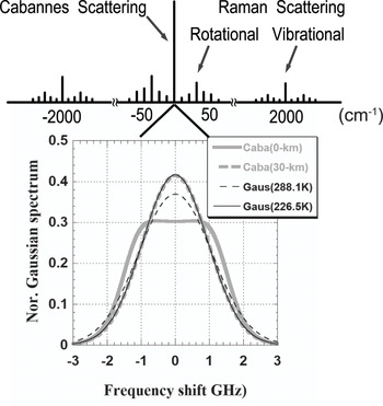
Cabannes spectra along with their Gaussian estimates are shown on an expanded frequency scale in the lower panel of Fig. 1.2. It is well known that at thermal equilibrium the scattering spectrum from a gas is Doppler broadened, giving rise to a Gaussian spectrum with full width at half-maximum (FWHM) depending on the gas temperature. These are shown as black thin-dashed and solid lines in the lower part of Fig. 1.2, respectively corresponding to atmosphere at 288.15 K (mean temperature at sea level) and at 226.15 K (mean temperature at 30 km altitude). Comparing the Cabannes spectra, gray thick solid and dashed lines, of atmospheric scattering at altitudes of 0 km (288.15 K, 1 atm) and 30 km (226.15 K, 0.012 atm), respectively, we see that the sea-level Cabannes spectrum is not Gaussian, whereas at 30 km it is virtually indistinguishable from a Gaussian. The reason that the Cabannes scattering at sea level is not Gaussian is that in addition to temperature (entropy) fluctuations, the molecular ensemble is subject to pressure fluctuations due to collisions. Atmospheric pressure fluctuations, responsible for sound wave propagation, give rise to Brillouin scattering, resulting in a scattering angle-dependent frequency shift.

For backscattering, which is of interest here, the magnitude of the mean scattering wave vector is twice that of the incident wave vector. This means the wavelength of the backward propagating (sound or perturbation) wave in the atmosphere equals half of the incident optical wavelength (i.e., $\Lambda =\lambda /2$). Thus, the mean Brillouin frequency shift is 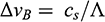$\Delta {\nu }_B=c_s/\Lambda$, where $c_s$ is the speed of sound. For atmosphere at 288 K at sea level, 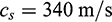$c_s=340\text{m/s}$, which for $\lambda =532\text{nm}$ results in a frequency shift of $\Delta {\nu }_B=1.28\text{GHz}$.

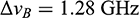While a more thorough description of the Cabannes spectrum will be given in Chapter 4, an oversimplified account describes the atmospheric Cabannes spectrum as the result of translational motion of the molecules. In the absence of collisions, molecules in thermal equilibrium move independently and randomly, giving rise to a Doppler-broadened Cabannes line. As pressure increases, the chance of colliding with other molecules increases. This allows the molecules to move correlatively and sound waves to propagate, which diverts part of the scattering power to the Brillouin wings, with two sidebands centered at 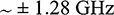$~\pm 1.28\text{GHz}$ for 1 atm, in the backward direction. The relative contribution of the sidebands (Brillouin scattering) is determined by a comparison between the scattering wavelength, 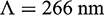$\Lambda =266\text{nm}$, and the mean free path between collisions $\overline{\ell }$. A simple calculation yields a mean free path of 66 nm at sea level and 44,000 nm at 30 km. Thus, at sea level many collisions occur within one scattering wavelength, which makes the Cabannes spectrum much broader (shown as the gray solid curve), while at 30 km $\overline{\ell }\gg \Lambda$, the Cabannes spectrum (thin black solid curve) appears to be identical to the associated Doppler-broadened spectrum (thick gray dashed curve). The details of nonresonant light scattering from linear molecules, their spectral distribution and relative line strengths, will be treated quantum mechanically in more detail in Chapter 4.

Lidar remote sensing of the atmosphere began in 1954 with the use of searchlights for the study of atmospheric temperature, density, and pressure in the altitude range between 10 and 68 km [Reference Elterman1.7]. Soon after the invention of the ruby laser in 1960, the first Rayleigh–Mie, differential absorption, Raman, and fluorescence lidar observations were reported between 1969 and 1970. Since that time, lidar remote sensing of the atmosphere has become increasingly active. A selected collection of milestone papers on the achievements during the first three decades was published in 1997 [Reference Grant, Browell, Menzies, Sassen and She1.8]. We hope with this book to cover the fundamentals that made those achievements, as well as those in the years that followed, possible. For this objective, we have made no attempt to include an exhaustive list of relevant publications in the literature; rather, we refer to selective publications that allow us to explain the physics fundamentals for the atmospheric lidars in question.