6.1 Introduction

Soil depth is a fundamental property of soils. Sensitivity tests have shown that uncertainty in our knowledge of soil depth is a significant contributor to uncertainty in estimating carbon and water fluxes between the terrestrial environment and the atmosphere (Knorr and Lakshmi, Reference Knorr, Lakshmi, Lakshmi, Albertson and Schaake2001; Peterman et al., Reference Peterman, Bachelet, Ferschweiler and Sheehan2014), and thus the soil moisture and the biosequestration potential of the terrestrial environment.

Yet even something as apparently simple as soil depth can be difficult to define objectively, as the definitions discussed in the previous chapter for regolith, soils and saprolite indicate. The models described below define soil as all materials above the unweathered bedrock or saprolite, so soil depth is that depth to the bedrock or saprolite interface. In the field such a distinct boundary may or may not exist. For instance, the regolith may contain significant corestones surrounded by soil, and the corestones may become bigger and more frequent with depth until there is a transition to solid bedrock (e.g. Fletcher et al., Reference Fletcher, Buss and Brantley2006; Graham et al., Reference Graham, Rossi and Hubbert2010). Measurements of changes in porosity and bulk density down through the soil profile in the field show mixed results even when allowing for the impacts of agricultural landuse. Some profiles show no significant change down the soil profile suggesting that all change occurs at the base of the profile (e.g. Angers et al., Reference Angers1997; Corti et al., Reference Corti, Agnelli, Certini and Ugolini2001), while others show a trend of increasing bulk density with depth suggesting that changes may occur gradually throughout the profile (e.g. Unger and Jones, Reference Unger and Jones1998; Graham et al., Reference Graham, Rossi and Hubbert2010). Ouimet (Reference Ouimet2008) noted a sharp boundary in bulk density within his profiles and attributed this to tree throw physically mixing (i.e. bioturbation) the soil. Finally, Richter and Markewitz (Reference Richter and Markewitz1995) report a gradual transition in the soil biogeochemistry with depth and argue that physical properties underestimate the depth of the biochemically active zone. Despite these conflicting data the literature discussed in this chapter typically assumes that a distinct interface between saprolite and soil exists.

6.2 Soil Depth and Bedrock Conversion to Soil

Ahnert (Reference Ahnert1976) first described a model for the evolution of soil depth:

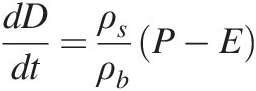
$\frac{\mathrm{dD}}{\mathrm{dt}}=\frac{{\rho }_s}{{\rho }_b}\left(P-E\right)$(6.1)

where D is the depth of the soil, P is the rate of conversion of bedrock to soil (depth/time), E is the erosion rate (depth/time) and ρ_s${\rho }_s$ and ρ_b${\rho }_b$ are the bulk densities of the soil averaged over depth and bedrock density at the soil-bedrock interface, respectively. Some early equations ignore changes in porosity and bulk density that occur in the conversion from bedrock to soil. Equation (6.1) includes this bulk density change. Ahnert did not consider bulk density changes resulting from soil production but they are included above for consistency with Chapter 2. The general form of Equation (6.1) (either with or without the density change) is the basis of all the soil depth modelling that has followed on from Ahnert.

This equation ignores the effect of dissolution because, as we see when we discuss bulk density evolution (Section 7.6), there is the possibility of complex interactions between dissolution and bulk density changes. However, in a model of chemical dissolution in soil Mudd and Furbish (Reference Mudd and Furbish2004) and Yoo and Mudd (Reference Yoo and Mudd2008) assumed that bioturbation would mix the soil from top to bottom and ensure that bulk density remained the same throughout the profile (Brimhall et al., Reference Brimhall, Chadwick, Lewis, Compston, Williams, Danti, Dietrich, Power, Hendricks and Bratt1992). Brimhall et al. (Reference Brimhall, Chadwick, Lewis, Compston, Williams, Danti, Dietrich, Power, Hendricks and Bratt1992) found a complex pattern of dilation (e.g. increase in porosity) and collapse (decrease in porosity) based on depth, age and mineralogy, and attributed many of the changes to bioturbation and related processes, which will be discussed in Chapter 7.

The function P is (interchangeably) called the bedrock conversion function, bedrock weathering function, bedrock erosion function or soil production function. In recent years the soil production function (SPF) has been the most commonly used description, and this is the terminology used in this book. If, as is commonly accepted, the SPF declines with the depth of the soil-bedrock interface below the surface, then an equilibrium depth can be attained. A particularly simple solution arises when the ‘exponential’ SPF is used:

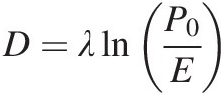
where P₀$P_0$ is the soil production rate when there is zero soil coverage, λ$\lambda$ is the rate at which the conversion rate decreases with increasing soil depth and z is the depth below the soil surface. For equilibrium when the left-hand side of Equation (6.1) equals zero,

where D is the depth below the surface of the bedrock interface (i.e. the soil depth), or rearranging

$D=\lambda ln\left(\frac{P_0}{E}\right)$(6.4)

This equation shows that if the SPF and erosion rates are the same everywhere, then the soil depth will also be the same everywhere. Also if the SPF rate increases or the erosion rate decreases, then the soil depth will increase. Since it is rare for soils to be constant depth everywhere, one of the conversion or erosion rates must vary in space if Equation (6.4) is to be true. Equation (6.4) also says that everything else being equal, then higher erosion rates should lead to shallower soils, which has been observed in the field (Cox, Reference Cox1980; Dietrich et al., Reference Dietrich, Reiss, Hsu and Montgomery1995; Heimsath et al., Reference Heimsath, Dietrich, Nishiizummi and Finkel1999).

The conceptual appeal of the exponential form of the SPF is that the conversion rate decreases with the depth of the bedrock interface below the soil surface. If soil production is driven by temperature (e.g. driving cycles of internal thermal stresses in rock particles) and soil wetness variations (e.g. driving cycles of salt crystallisation), both of which become less extreme with depth in the soil profile, this function is qualitatively consistent with observed behaviour. Recent research using cosmogenic nuclides for the dating of soil profiles has provided strong empirical evidence that, to first order, the exponential decline with depth in Equation (6.2) is well founded (Heimsath et al., Reference Heimsath, Dietrich, Nishiizummi and Finkel1997, Reference Heimsath, Dietrich, Nishiizummi and Finkel1999). There do, however, appear to be significant variations in both P₀$P_0$ and λ$\lambda$ from site to site (Anderson et al., Reference Anderson, Dietrich and Brimhall2002). Recent field research has clarified some causal factors for variations from site to site (Navarre-Sitchler et al., Reference Navarre-Stichler, Cole, Rother, Jin, Buss and Brantley2013) with

• the underlying geology and soil moisture being highlighted as dominant and

• less clear-cut conclusions on the role of temperature, with some authors showing a strong impact (e.g. Eppes and Griffing, Reference Eppes and Griffing2010) while others show a relatively minor impact for sites below the snowline (e.g. Rasmussen et al., Reference Rasmussen, Dahlgren and Southard2010).

There are other postulated SPFs. One criticism of the exponential function is that it has the highest weathering rate when there is no soil. If weathering is also driven by the time that the rock is wet (e.g. by chemical reactions), then the rate should be highest just below the surface when there is sufficient soil to store some of the infiltrated water (Carson and Kirkby, Reference Carson and Kirkby1972). To model this, the “humped” function was developed (Figure 6.1). A variety of mathematical forms have been presented (e.g. Ahnert, Reference Ahnert1977; Anderson, Reference Anderson2002), all of which are empirical. While Heimsath et al. (Reference Heimsath, Hancock and Fink2009) and Stockmann et al. (Reference Stockmann, Minasny and McBratney2014) provided experimental evidence which supports the exponential function, their data are also consistent with humped behaviour because there is significant scatter in their data for shallow soil depths.

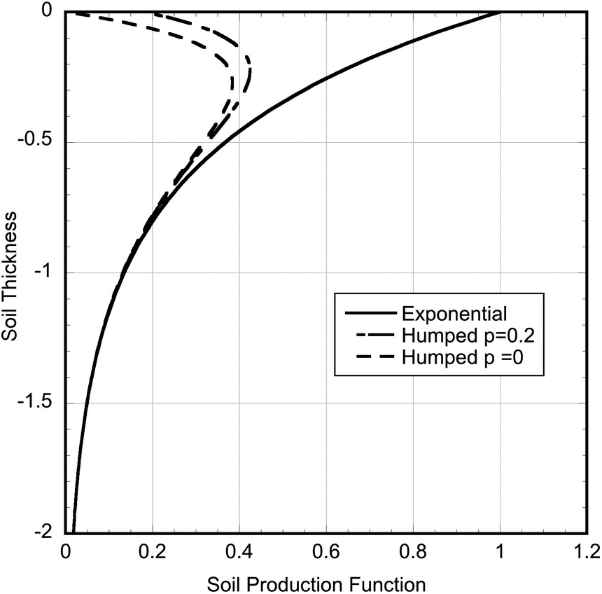
Figure 6.1: Example exponential and humped soil production functions (SPFs). Two humped functions are shown: (a) p = 0$p=0$ is zero at the soil surface, (b) p = 0.2$p=0.2$ is nonzero at the soil surface; all other parameters are the same. The depth decay parameter is the same for all three functions (i.e. λ = δ₂$\lambda ={\delta }_2$), so, in this example, the exponential and humped functions converge to the same value for deeper soils.

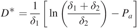
The key differences between the mathematical formulations of the humped SPF are whether (1) the function goes to zero or not, for zero soil depth (i.e. whether a bare rock surface can weather at all), (2) it asymptotes to zero for large depths (i.e. weathering declines to zero at depth like the exponential function) and (3) the function is continuously differentiable over its range (differentiability can be useful for numerical solvers). Many of the published equations do not meet the third point because they provide different equations for above and below the depth of maximum weathering rate. One equation that satisfies all three requirements is a modification of that used by Minasny and McBratney (Reference Minasny and McBratney2006) and Cohen et al. (Reference Cohen, Willgoose and Hancock2010):

where δ₁,${\delta }_1,$ δ₂${\delta }_2$ and P_a$P_a$ are all parameters with positive values, where δ₁ > δ₂,${\delta }_1>{\delta }_2,$ and P_a$P_a$ controls the weathering rate for zero soil depth. The depth D^∗$D^{\ast }$ at which maximum weathering rate occurs is

$D^{\ast }=\frac{1}{{\delta }_1}\left(ln\left(\frac{{\delta }_1+{\delta }_2}{{\delta }_2}\right)-P_a\right)$(6.6)

Furbish and Fagherazzi (Reference Furbish and Fagherazzi2001) present another equation, but it has the disadvantage that it cannot control the rate of decline with depth (i.e. the δ₂${\delta }_2$ in Equation (6.5)) independently of the weathering rate at the surface (i.e. P_a$P_a$ in Equation (6.5)), so we will not discuss it. Finally some studies suggest that soil production rates are independent of depth (Wilkinson et al., Reference Wilkinson, Humphreys, Chappell, Fifield and Smith2003), though they are in the minority and the reasons for their observed behaviour is not known.

All these equations are empirical and based on field experiment data including cosmogenic nuclide dating (CN), optically stimulated luminescence (OSL) dating and geochemical modelling of rivers and soil profiles (Minasny et al., Reference Minasny, Finke, Stockmann, Vanwalleghem and McBratney2015). One consideration with the dating methods is they rely upon assumptions about rates of exposure to the atmosphere. Bioturbation potentially mixes the soil, bringing deeper material to the surface and burying surface material. If the soil is fully mixed from top to bottom, then the cosmogenic dating methods will yield the average age of the soil, whereas OSL will yield the time since the particle(s) were last at the surface (Dunai, Reference Dunai2010).

One of the limitations of the SPF above is that they lack any explicit feedbacks with soil moisture and temperature. The work of Freer et al. (Reference Freer, McDonnell, Beven, Peters, Burns, Hooper, Aulenbach and Kendall2002) provides empirical evidence of the importance of spatial feedbacks that are not included in the above formulations. They mapped the bedrock topography and soil depth at the Panola site and showed that the spatial pattern of the bedrock topography and soil depth appeared to be unconnected to the surface topography. The bedrock surface had patterns of drainage with valleys and holes in the bedrock surface suggestive of concentrated water flow over the bedrock surface (James et al., Reference James, McDonnell, Tromp-van Meerveld and Peters2010). This disconnect between the surface topography and the bedrock topography, but where the patterns were clearly not random nor linked to geology, suggested feedbacks in the soil thickness dynamics that cannot be modelled by the simple models above.

Saco et al. (Reference Saco, Willgoose and Hancock2006) investigated whether the bedrock patterns observed at Panola are a result of soil water where the lateral soil water drainage patterns are determined by the bedrock topography, not the soil surface topography. They extended the exponential SPF by making it a function of soil moisture so that the SPF became

where M is the soil moisture as determined by using the wetness index

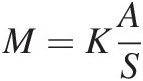$M=K\frac{A}{S}$(6.8)

but where the contributing area A and slope S used in the wetness index formulation were derived from analysing the bedrock topography rather than, as is traditionally done, the soil surface topography. Depending on the functional relationship between soil moisture and weathering used (i.e. the functional form of f(M)$f\left(M\right)$, e.g. using absolute depth of soil water versus percentage saturation of the soil profile) spatial patterns in the bedrock topography and soil depth qualitatively similar to that observed by Freer could be generated (Figure 16.1).

There are ecological feedbacks that I will touch on briefly here but will return to later in the book. In arid zones where the vegetation spatial distribution is banded, it has been observed (Ludwig et al., Reference Ludwig, Wilcox, Breshears, Tongway and Imeson2005) that infiltration was higher (and therefore so was soil moisture) within the bands of vegetation (enhanced organic matter changed the soil structure and increased the infiltration capacity) than between the vegetation bands. Underneath the bands of vegetation the soil depth was greater than in the interband areas where there was lower soil moisture and organic matter. The model formulations of Saco et al. (Reference Saco, Willgoose and Hancock2006, Reference Saco, Willgoose and Hancock2007) are consistent with this behaviour.

Gabet and Mudd (Reference Gabet and Mudd2010) have proposed a tree throw mechanism that results in a distinct soil-saprolite boundary, a distinct change in bulk density at this boundary and which naturally leads to a humped SPF. In essence tree roots rip out rock from the saprolite during tree throw. This causes the distinct boundary and bulk density change at the soil-saprolite interface. The humped SPF results from an interaction between an exponential decline in root density in depth, and an increasing density of trees as soil depth increases (Figure 6.2). The model has been tested in a heavily forested wet climate (Figure 6.3). Finke et al. (Reference Finke, Vanwalleghem, Opolot, Poesen and Deckers2013) modelled tree throw as a hypothesis for explaining the apparent random variability in soil depth and lack of any spatial organisation in soil cores at an aeolian site in Belgium (Vanwalleghem et al., Reference Vanwalleghem, Poesen, McBratney and Deckers2010). A model with tree throw was an improvement over a model without tree throw, though the improvement was relatively small.

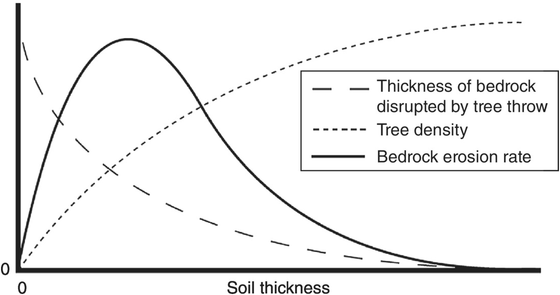
Figure 6.2: As soil thickness increases, the amount of bedrock disrupted by tree roots decreases because of their limited vertical extent. Conversely, thicker soils support higher tree densities. The combination of these two competing trends is posited to produce a humped soil production function.

(Figure 2 from Gabet and Mudd, Reference Gabet and Mudd2010)

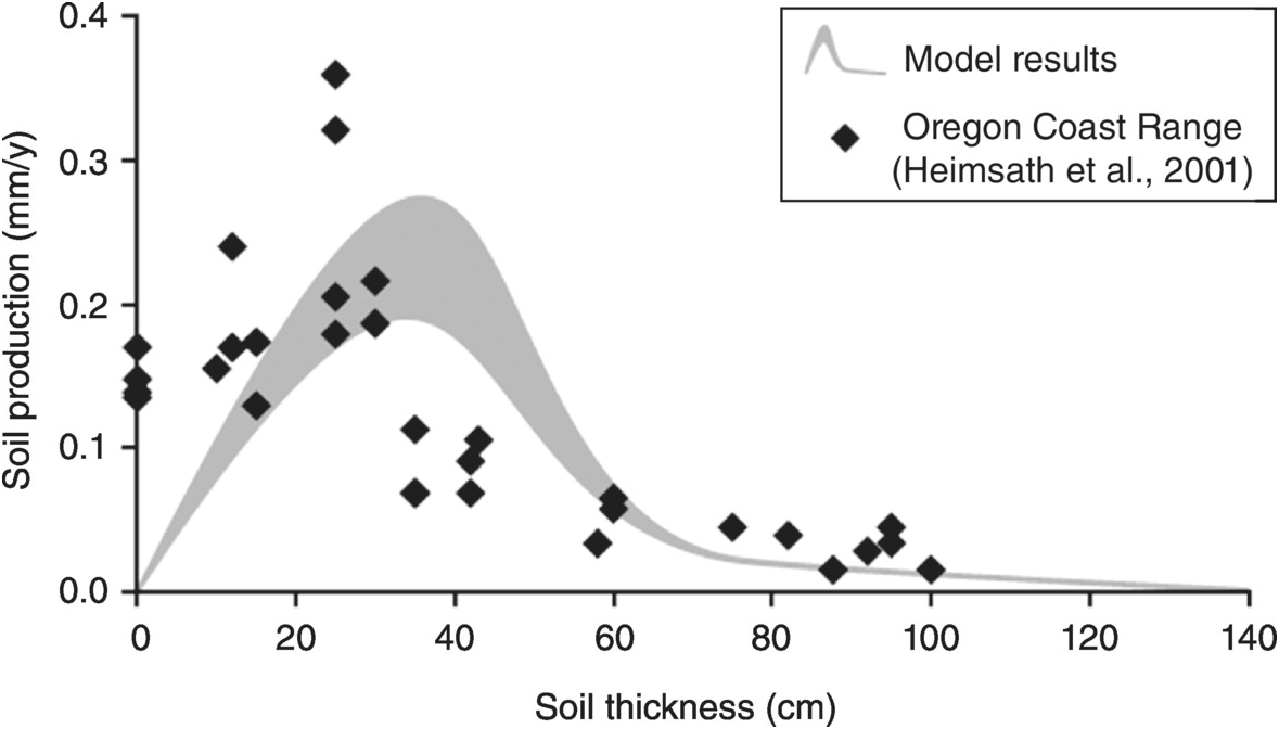
Figure 6.3: Model results compared to soil production rates measured in a Douglas fir forest in the Oregon Coast Range. The results of Gabet and Mudd, (Reference Gabet and Mudd2010) (their Figure 6) bracket the shaded area. Both the data and the model results reveal a humped relationship between bedrock erosion rates and soil thickness.

(Figure 7 from Gabet and Mudd, Reference Gabet and Mudd2010)

One final observation on the SPFs is on the stability of the equilibrium solutions to the soil depth equation. Kirkby (personal communication) has pointed out that the solution in Equation (6.4) for the exponential function is unconditionally stable for all soil depths, so that any soil, if at the equilibrium in Equation (6.4), will return to this equilibrium if the soil depth is perturbed slightly (this return to the previous solution is the mathematical definition of stability, with respect to soil depth). The humped function, however, is not unconditionally stable everywhere (Figure 6.4). For soil depth greater than the hump peak D^∗$D^{\ast }$ (Equation (6.6)) the soil depth solution is stable. However, for soil depths between zero and the hump peak, the equilibrium solution for soil depth is unstable. In this region if the soil depth is slightly increased, then the SPF increases and the soil depth increases further. This continues until the soil depth reaches the hump peak, and the soil depth will evolve past the peak (because at the hump peak soil production is greater than the erosion rate) until it reaches the corresponding equilibrium soil depth greater than D^∗,$D^{\ast },$ and vice versa if the soil depth is slightly decreased, then the soil production function decreases and the soil thins further. Again this will continue until the soil depth is zero (the rock exposure likely turning that part of the hillslope into a weathering- or detachment-limited regime).

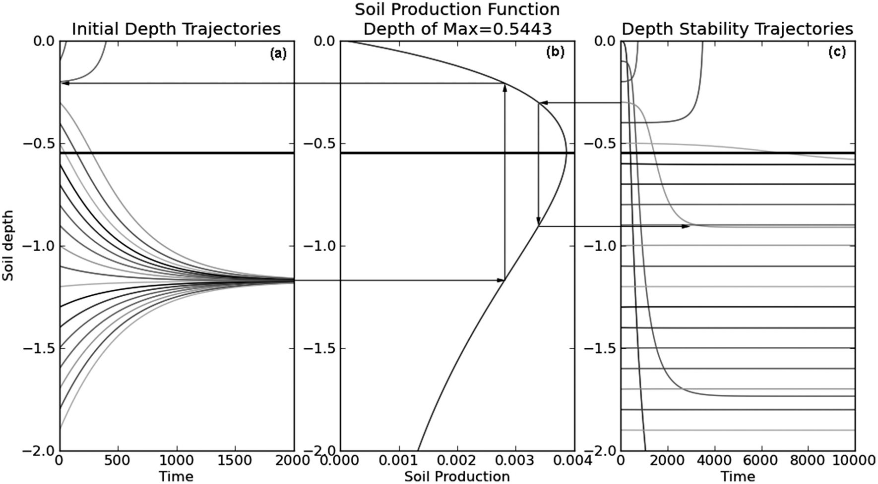
Figure 6.4: Trajectories over time of soils with a range of initial soil depths and subjected to the humped soil production function. (a) All simulations have the same erosion rate for each initial soil depth and trajectory with time; (b) the soil production function applied in this example and (c) each initial soil depth has an erosion rate just balancing the corresponding soil production rate for that initial soil depth. In panel (c) a small random perturbation on this erosion rate (±0.5% the erosion rate) is then applied, and this panel shows the subsequent trajectory of the soil depth.

Figure 6.4 shows an example of the soil depth evolution for a range of initial soil depths (in increments of 0.1 m from 0.1 m to 2.0 m) and the humped SPF in Equation (6.5). The same erosion is applied to all the trajectories so soils grow deeper or shallower based on the imbalance between the erosion and the soil production for that depth. In this example most of the initially deeper soils evolve to an equilibrium depth of 1.17 m (the exact value of the equilibrium depth is a function of the parameters used in the SPF, 1.17 m is the solution for the parameters used in Figure 6.4). Figure 6.4a shows if you project across to the SPF in Figure 6.4b, that the equivalent shallow depth equilibrium with the same soil production rate is 0.21 m. All soils with initial depth less than 0.21 m (i.e. in the figure the 0.1 m and 0.2 m initial soil depths) diverge away from the equilibrium to have zero depth, while soils with an initial depth of greater than 0.21 m converged past the hump to the deeper equilibrium. This means that in practice while a solution for soil depth between zero depth and D^∗$D^{\ast }$ is mathematically possible it is unstable, and the solution will diverge from this equilibrium toward either zero depth or the stable depth on the other side of D^∗.$D^{\ast }.$

Figure 6.4c shows a slightly different but equally enlightening set of depth trajectories for the same SPF in Figure 6.4b. In this figure for each initial depth, the erosion rate that would exactly balance the soil production rate has been calculated. If the soil production and erosion exactly balance, then the soil depth will not change with time, but if the equilibrium is unstable, tiny perturbations will grow and eventually cause the depth to diverge from the equilibrium and converge on the stable equilibrium. To trigger this divergence, a small (±0.05%) random perturbation on the erosion rate was applied so some erosion rates will be slightly higher (i.e. so soils will initially thin slightly) while others are slightly smaller (so soils will initially thicken slightly) than the exact equilibrium. Figure 6.4c shows that for soils depths greater than the hump, the trajectory is a straight line because they are a stable equilibrium and slight perturbations do not make significant difference in the equilibrium soil depth. However, for all the depths less than the hump there is divergence. Some of the trajectories converge on zero. These are the cases where the random perturbations produced an erosion rate slightly higher than equilibrium so soils thin. Some of the other trajectories increase and converge on the equilibrium soil depth that is at greater depth than the hump. For instance, projecting across to the SPF in Figure 6.4b, the trajectory starting at 0.4 m converges on the equilibrium at about 0.9 m. The zero depth simulation in also interesting because the parameters chosen for the SPF have a nonzero value at depth zero and the random perturbation results in a reduced erosion rate. Because the erosion is very small, the balancing soil production rate is also very small, and they only balance when the depth is off-scale at the bottom (about 8 m in this case). This is the reason the zero depth simulation disappears off-scale at time 1000.

Carson and Kirkby (Reference Carson and Kirkby1972, p. 105) and Kirkby (Reference Kirkby, Abrahart, Openshaw and See2000) speculated that these stable/unstable equilibria will lead to a hillslope that is a patchwork of bare rock and soil with depths greater than D^∗$D^{\ast }$ and is potentially a factor in badland development. Figure 6.4c supports that idea because even with identical physics minor random perturbations caused some soils to disappear and some to deepen. This argument is true for any shape SPF where there is a region where the SPF increases with increasing depth, so is more general than the exact form of Equation (6.5) and the example in Figure 6.4. To further investigate this hypothesis Furbish and Fagherazzi (Reference Furbish and Fagherazzi2001) coupled the humped SPF with diffusive and fluvial hillslope transport and showed that the spatial coupling does not substantially change the hillslope profile at the hilltops but may lead to significant changes downslope where fluvial transport is dominant.

The key characteristics of the models in this chapter are that they only simulate the processes that are occurring at the top and bottom of the soil profile and use these processes to determine the mass balance of the soil profile, lumped as a whole from top to bottom, to describe the dynamics. However, much weathering occurs within the profile (e.g. Anderson et al., Reference Anderson, Dietrich and Brimhall2002), so focussing on the top and the bottom of the profile is a simplification. More importantly these models do not describe what the characteristics are of the soil that is created, and they do not provide any information about what is occurring within the soil profile. We will now discuss models that simulate the evolution of soil characteristics within the profile.