


1. INTRODUCTION
The Larsen Ice Shelf, located to the east of the Antarctic Peninsula, has exhibited a persistent, stepped retreat since aerial observations began in the 1950s, with significant retreat since 1986 (Fig. 1; Cooper, Reference Cooper1997; Ferrigno and others, Reference Ferrigno2008; Cook and Vaughan, Reference Cook and Vaughan2010). Between January and March 1995, the majority of the Larsen A Ice Shelf collapsed, co-incident with the collapse of the Prince Gustav Ice Shelf and a large calving event from the Larsen B Ice Shelf (Rott and others, Reference Rott, Skvarca and Nagler1996). The floating area of the Larsen A Ice Shelf reduced by half during the last week of January 1995 alone, and by 8 March 1995, covered only 18% of its previous extent (Rott and others, Reference Rott, Rack, Stuefer and Skvarca1997; Skvarca and others, Reference Skvarca, Rack, Rott and Ibarzábal y Donángelo1999). At the time of collapse, there was considerable debate regarding the role of lateral buttressing in flow dynamics, specifically the nature of grounding line dynamics following a significant perturbation such as the loss of an ice shelf (e.g. Weertman, Reference Weertman1974; Hindmarsh, Reference Hindmarsh1993; Hindmarsh and Le Meur, Reference Hindmarsh and Le Meur2001; Ritz and others, Reference Ritz, Rommelaere and Dumas2001; Dupont and Alley, Reference Dupont and Alley2005). Observations following the Larsen A collapse confirmed the significant and rapid effect of this event on the flow dynamics of tributary glaciers, with far-reaching effects upstream (Rott and others, Reference Rott, Rack, Skvarca and Angelis2002, Reference Rott2014; De Angelis and Skvarca, Reference De Angelis and Skvarca2003; Shuman and others, Reference Shuman, Berthier and Scambos2011). Previous modelling studies of Larsen A considered the conditions and possible mechanisms for the break-up of the ice shelf (Doake and others, Reference Doake, Corr, Rott, Skvarca and Young1998; Scambos and others, Reference Scambos, Hulbe, Fahnestock and Bohlander2000; Vieli and others, Reference Vieli, Payne, Shepherd and Du2007; Albrecht and Levermann, Reference Albrecht and Levermann2014), but did not consider the whole ice-sheet ice-shelf system including observed changes in buttressing and velocity and the effects upstream of the grounding line within tributary glaciers. The collapse of Larsen A provides one of the few examples in glaciology, where model validation can be performed.
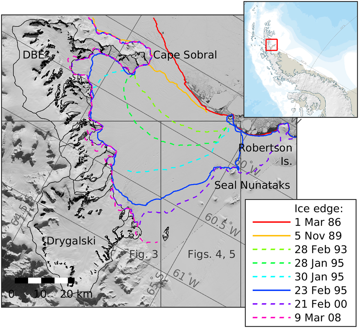
Fig. 1. Area of interest showing ice shelf extents (solid and dashed coloured lines; Skvarca and others, Reference Skvarca, Rack, Rott and Ibarzábal y Donángelo1999; Ferrigno and others, Reference Ferrigno2008) and ice catchments (thin black lines; Cook and others, Reference Cook, Vaughan, Luckman and Murray2014). Inset displays the location on the Antarctic Peninsula using a basemap from the SCAR Antarctic Digital Database 6.0. Base image is Landsat from 1 Mar 1986. Figures are plotted using WGS84 Antarctic Polar Stereographic projection with Standard Parallel at − 71 °S.
Surface velocities of Larsen A tributary glaciers upstream of the grounding line increased significantly within 8 months of the collapse, from 200 m a−1 at the outlets of Drygalski and Dinsmoor-Bombardier-Edgeworth (DBE) glaciers to over 900 m a−1 by austral spring 1995 (Fig. 2; Bindschadler and others, Reference Bindschadler, Fahnestock, Skvarca and Scambos1994; Rack and others, Reference Rack, Rott, Siegel and Skvarca1999; Rott and others, Reference Rott2014; Seehaus and others, Reference Seehaus, Marinsek, Helm, Skvarca and Braun2015) and continued accelerating for at least 5 a post collapse (Rott and others, Reference Rott2014). This acceleration resulted in dynamic thinning and mass loss: in total, the mass loss from former Larsen A tributaries has contributed 17–18% of the mass loss from the northern Antarctic Peninsula (Scambos and others, Reference Scambos2014).

Fig. 2. Observed surface speeds from ERS-1 DInSAR pairs and model mesh extents (a) acquired 8 December 1992–16 February 1993 (Seehaus and others, Reference Seehaus, Marinsek, Helm, Skvarca and Braun2015) with inset displaying the 6-node mesh and (b) acquired 31 October – 5 November 1995 (Rott and others, Reference Rott2014). The model no-flow boundaries (thick black line), free-slip boundaries (thick grey line) and open boundaries (thick coloured lines, with colours relating to Fig. 1 for before and after the ice-shelf collapse respectively) are shown. Base images are Landsat, from 1 March 1986 and 31 December 2001, the latter acquired some time after the ice-shelf collapse.
Recent reanalysed velocity datasets (Rott and others, Reference Rott2014; Seehaus and others, Reference Seehaus, Marinsek, Helm, Skvarca and Braun2015) and new developments in inversions for bed elevation (Huss and Farinotti, Reference Huss and Farinotti2014) now enable high-resolution modelling of the former Larsen A Ice Shelf region including an investigation of the effects of a reduction in ice-shelf buttressing. Here, we use a numerical ice flow model of a type commonly used in glaciology to quantify future changes in flow due to changes following collapse in January 1995. We then compare these numerical results with remote-sensing observations of velocity obtained shortly after the collapse. Besides providing new insights into the effect of the ice-shelf collapse on ice-shelf buttressing, we are thereby able to test the performance of the numerical model against observations.
This paper demonstrates with a real-world example, the instantaneous effect that removing buttressing has on upsteam flow. Section 2 describes the numerical model and datasets used. We demonstrate that the observed glacier velocity speed up near the grounding line can be replicated well by modelling only the change in the ice shelf extent (Section 3). We discuss the modelled change in backstress due to the ice-shelf collapse, its effect on the acceleration of tributary glaciers in the vicinity of the grounding line and discrepancies between the modelled and observed data (Section 4). These discrepancies are discussed in the context of model limitations, transient effects and alternative contributing mechanisms on glacier acceleration of the order of 10 km upstream.
2. METHODOLOGY
We use an ice flow model to calculate the instantaneous changes in flow due to the collapse of Larsen A Ice Shelf. Ice flow, as calculated by the model, is primarily a function of geometry and model parameters describing basal sliding (slipperiness, C) and internal ice deformation (rate factor, A). These two distributed parameter sets were determined from measurements of ice flow using inversion techniques.
2.1. Numerical model
The numerical ice flow model, referred to as Úa, solves the shallow shelf approximation (SSA) equations in two-horizontal-dimensions (2HD) on a finite-element mesh. Úa has been tried-and-tested in all recent model intercomparison exercises (Pattyn and others, Reference Pattyn2012, Reference Pattyn2013) and in real world settings (Favier and others, Reference Favier2014; De Rydt and others, Reference De Rydt, Gudmundsson, Rott and Bamber2015), and is described by Gudmundsson and others (Reference Gudmundsson, Krug, Durand, Favier and Gagliardini2012).
The computational domain was discretised using linear, quadratic and cubic elements with sizes ranging from 100 to 1000 m, with the finest resolution applied around grounding lines.
The model parameters basal slipperiness and rate factor were determined using commonly used inversion methods (MacAyeal, Reference MacAyeal1992, Reference MacAyeal1993), each with nonlinear exponents, m = 3 and n = 3.
2.2. Model geometry
We used the ice edge extents determined by Ferrigno and others (Reference Ferrigno2008) for periods from March 1986 to February 1995 to define the model geometries prior and post collapse (Figs 1, 2; data sources are listed in Table 1). Along the calving fronts the (vertically integrated) hydrostatic ocean pressure was applied. Along the furthermost upstream boundaries, velocities were set to zero. The model domain included several nunataks (SCAR Antarctic Digital Database 6.0 http://www.add.scar.org), and these ice-free regions were represented as holes in the finite-element mesh. Along such inner boundaries, a free-slip boundary condition was applied, where normal velocities were set to zero while the ice was allowed to move freely in tangential direction.
Table 1. Data sources

For the Antarctic Peninsula, surface topographic data at 100 m resolution has recently been published revisiting ASTER data (Cook and others, Reference Cook, Murray, Luckman, DG and Barrand2012). Unfortunately, the ASTER GDEM is derived from data acquired during the period 2000–09 but the acquisition date(s) used for each region have not been retained with the DEM and the data masked to the 2008 ice edge. Significant elevation changes have occurred since the ice-shelf collapse in 1995 and there appear to be several inconsistencies in the ASTER dataset between elevation and grounding line positions. Surface elevation required for hydrostatic equilibrium at the grounding line at Drygalski Glacier (from February 1996; Rignot and others, Reference Rignot, Mouginot and Scheuchl2011) is 100 m above the ASTER GDEM surface elevation.
Having considered, and discounted, various possible modifications to the ASTER GDEM to arrive at a realistic elevation distribution around observe grounding lines, we instead used RAMP ice-surface data (an integration of elevation data acquired to 1999; Liu and others, Reference Liu, Jezek, Li and Zhao2001) in the region of grounded ice, supplemented by ERS-1 reanalysed altimetry data for the ice-shelf region (Gilbert and others, Reference Gilbert2014). The ERS-1 altimetry was corrected for the geoid to make consistent with the surface and bedrock data, and for the tide using the CATS model v2.01 (Padman and others, Reference Padman, Fricker, Coleman, Howard and Erofeeva2002).
Bedrock data recently calculated by Huss and Farinotti (Reference Huss and Farinotti2014) at a high-horizontal resolution of 100 m was tied in to bathymetry from IBCSO (Arndt and others, Reference Arndt2013). Ice thickness was determined from the difference between the surface and bedrock data, with areas of floatation and hence the ice-shelf base determined from hydrostatic equilibrium arguments. In the floatation point calculation, the density of ice was estimated allowing for firn thickness and density determined by Ligtenberg and others (Reference Ligtenberg, Helsen and van den Broeke2011). The surface elevation, bathymetry and ice thickness was checked for consistency with the observed location of the grounding line before the ice-shelf collapse and from this assessment, we concentrate on the results for Drygalski Glacier.
2.3. Surface velocities
We used surface velocity datasets obtained from differential interferometry both prior and post collapse. The pre-collapse velocities were determined by Seehaus and others (Reference Seehaus, Marinsek, Helm, Skvarca and Braun2015) from pairs acquired between 8 December 1992 and 16 February 1993 and the post-collapse velocities were determined by Rott and others (Reference Rott2014) from pairs acquired between 31 October 1995 and 5 November 1995 (Fig. 2).
3. RESULTS
3.1. Replicating post-collapse velocities
Following the model inversion routine for the post-collapse state that initialised the model parameters for the grounded ice, model discrepancies were mostly small compared with the observed surface velocities (Fig. 3). The mean difference between modelled and observed speed across the whole domain is −42.6 m a−1 and the RMSE is 85.3 m a−1. (The mean observed post-collapse speed across the domain is 86.1 m a−1.)

Fig. 3. Model initialisation: The difference between the modelled and observed surface speed (m a−1) for Drygalski Glacier following the ice-shelf collapse, after running the model inversion routine (a) in plan view and (b) along the grounding line and calving-front defined from DInSAR acquired in February 1996 (Rignot and others, Reference Rignot, Mouginot and Scheuchl2011).
The biggest discrepancy of 40% between modelled and observed velocities was found upstream of the right-hand flank of the glacier adjacent to Sentinel Nunatak. The observed post-collapse velocity (Fig. 2b) peaked here at over 1000 m a−1 whereas the model predicted speeds around 600 m a−1. However, along the grounding line and calving-front of Drygalski Glacier the modelled speeds were very close to those observed (Fig. 3b), which gives confidence in model estimates of the flux from grounded ice to floating or calved ice contributing to sea level.
3.2. Change in the velocity field due to loss of ice-shelf buttressing
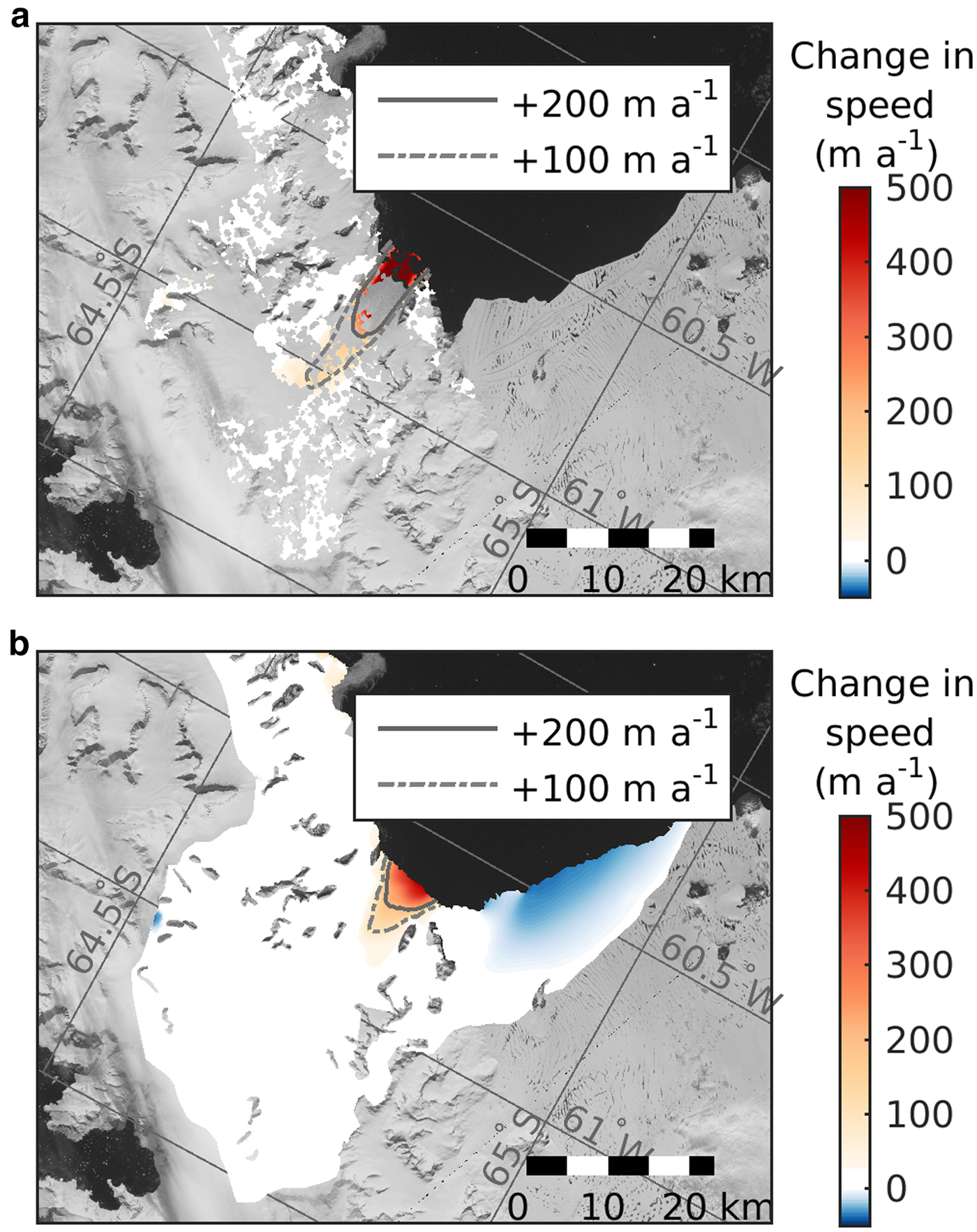
After the above described initialisation step, the model was re-run with the section of the ice shelf that collapsed in January–March 1995 removed. The observed speed up of Drygalski Glacier between periods before and after the ice-shelf collapse (Fig. 4a) was used to validate the modelled difference in speed (Fig. 4b).

Fig. 4. The increase in speed (m a−1) for Drygalski Glacier as a result of the collapse of Larsen A Ice Shelf (a) from observations (see Fig. 2) and (b) modelled by removing the ice-shelf geometry (from the 1989 extent to the 1995 extent). Note that the colour scale is saturated at 500 m a−1 to emphasise the upstream extent of the observed speed-up.
The maximum modelled increase in speed of 722 m a−1 compared well against the observed increase in speed of 763 m a−1. However, the spatial distribution of the speed up was not fully replicated by the model, with the modelled impact of the collapse not affecting the ice flow as far upstream as observed. As discussed below, this discrepancy is most likely due to dynamic effects because the model results present the instantaneous impact of the ice-shelf collapse on ice velocities and the post-collapse velocity data from late 1995, 8 months after the collapse took place.
4. DISCUSSION
4.1. Change in backstress due to ice-shelf collapse
There has been a recent impetus in the discussion of ice stream dynamics and marine ice-sheet stability in regard to the effect of buttressing (Goldberg and others, Reference Goldberg, Pollard and Schoof2009; Katz and Worster, Reference Katz and Worster2010; Gudmundsson, Reference Gudmundsson2013; Favier and others, Reference Favier2014). A metric of local buttressing attributable to the presence of the ice shelf is defined by Gudmundsson (Reference Gudmundsson2013), calculated as the difference between the pressure, which would be exerted by hydrostatic equilibrium and that pressure acting normal to the grounding line. Positive values of this backstress metric define areas where the hydrostatic pressure equivalent from the presence of an ice shelf is greater than the englacial stresses acting against the direction of the grounding line (or flow field) and negative backstress indicates areas where the englacial stresses along the grounding line are greater than the hydrostatic pressure at that point.
Along the outflow of Drygalski Glacier and at a number of other outflows along the Cape Worsley coast, the modelled backstress decreases consistently (up to −300 kPa) as a result of removing the ice shelf in the model (Fig. 5). Regions of a positive change in backstress are modelled where the ice shelf had flowed away from the grounding line ‘pulling’ the grounded ice out with it but after the ice-shelf collapse the ice flow was stagnant (the backstress increased from negative to zero). It is noted that the Seal Nunataks remnant ice shelf is modelled to slow down after the ice-shelf collapse (Fig. 4). The slow down in surface velocity can be explained by a change in the primary direction of flow between the cases with and without the ice shelf present. With the Larsen A Ice Shelf present, the outflow from Drygalski Glacier progresses outwards towards the ice shelf edge pulling adjacent regions of ice shelf with it. After the 1995 break-up the Seal Nunataks remnant ice shelf becomes static, and the area modelled to slow down calved or disintegrated within 6 a (Fig. 4; the background image is taken from December 2001 and demonstrates further ice-shelf collapse). The backstress exerted within the remnant ice shelf is in the main reduced following the 1995 break-up of the main ice shelf (Fig. 5). The exceptions are in the vicinity of pinning points where the stress field remains unchanged, and closer to the grounding line where parts of the remnant ice shelf exhibit a modelled increase in backstress because the englacial stresses are no longer affected by the inflow from Drygalski Glacier and instead are primarily forced by hydrostatic pressure.
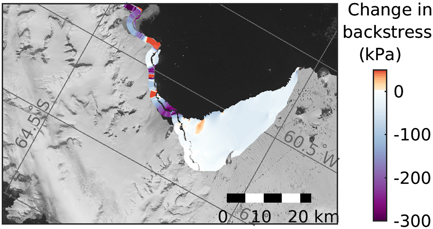
Fig. 5. The change in modelled backstress (kPa) for Drygalski Glacier and the remnant ice shelf at Seal Nunataks as a result of the collapse of Larsen A Ice Shelf. Backstress is calculated along the grounding line (thick offset line) and within the remnant ice shelf (colouring within the ice shelf), the latter calculated with the normal vector to the grounding line replaced with the normal vector to ice flow in Gudmundsson (Reference Gudmundsson2013).
4.2. Instantaneous and dynamic adjustment following ice-shelf collapse
The successful model prediction of change in speed in the vicinity of the grounding line (Fig. 4) demonstrates the significant and immediate effect of an abrupt change to the transmissive ‘membrane’ stresses acting across the grounding line on flow dynamics, highlighting the importance of explicitly including variations in the lateral transmissive stresses in model studies.
While a number of modelling studies have been published that account for changes in backstress, which can propagate upstream through transmissive horizontal lateral stresses (Joughin and others, Reference Joughin, Smith and Holland2010; Favier and others, Reference Favier2014; De Rydt and others, Reference De Rydt, Gudmundsson, Rott and Bamber2015), there are many studies that use a ‘flowline’ approach (Nick and others, Reference Nick, Vieli, Howat and Joughin2009, Reference Nick2012; Gladstone and others, Reference Gladstone2012; Goelzer and others, Reference Goelzer2013). It has been shown that flowline models are deficient in some circumstances including those more complex settings where buttressing effects are important (Gudmundsson and others, Reference Gudmundsson, Krug, Durand, Favier and Gagliardini2012; Gudmundsson, Reference Gudmundsson2013). While the flowline models may be supplemented by including lateral stress gradients and some parameterization of the lateral boundaries, they do not explicitly include variations in these lateral stresses from changes in the width of a glacier or changes in backstress at the glacier front. Gagliardini and others (Reference Gagliardini, Durand, Zwinger, Hindmarsh and Meur2010) discuss the complex behaviour of an ice-sheet ice-shelf system solving the full Stokes equations in plane flow. In that study, the lateral resistance of the ice shelf is accounted for by adding a body force in the momentum equation by a parameterisation on the flowline velocity. This provides sufficient variation to demonstrate interesting features in the model, but it obviously cannot accurately account for real-world variability in the lateral stresses. For regional studies attempting to predict future change, such as Nick and others (Reference Nick2013) and Barrand and others (Reference Barrand2013), it is difficult to ensure that the flow dynamics of each of the glacier catchments modelled and their evolution in time can be replicated by such flowline models. Barrand and others (Reference Barrand2013) discuss this issue, stating that their ‘forecasts over the early decades following break-up, therefore, will be subject to errors arising from ignoring membrane stresses’.
There remains a substantial change in speed observed upstream in the glacier channel, which the model does not capture (Fig. 4). For example, the contour of 200 m a−1 speed increase lies 12.1 km upstream of the grounding line in the observed data but only 4.6 km upstream in the model results. This remaining observed change in speed not predicted by the diagnostic model is likely to be due to dynamic adjustment of the glacier flow, for the reasons outlined below.
The post-collapse velocity observations were taken from a period 8 months after the ice shelf collapsed back to the ice edge position used in the model. Drygalski Glacier surface speed increased further between November 1995 and November 1999 (Rott and others, Reference Rott, Rack, Skvarca and Angelis2002) and dynamic thinning by glacier ‘surging’ was evident by a photographic survey conducted in October 2001 (De Angelis and Skvarca, Reference De Angelis and Skvarca2003). The timescale of the observed response is shorter than the timescale between the ‘fast’ and ‘slow’ forcing branches from perturbations discussed by Williams and others (Reference Williams, Hindmarsh and Arthern2012). Low frequency forcing or ‘slow’ perturbations lead to changes in flow at the grounding line and geometry that are able to propagate far upstream. High frequency forcing or ‘fast’ perturbations lead to a rapidly adjusted velocity but ‘thickness varies little and upstream propagation occurs through the direct transmission of membrane stresses’. Using the approach of Williams and others (Reference Williams, Hindmarsh and Arthern2012) for Drygalski Glacier assuming a length scale, X*, of 34.15 km, a mean thickness across the grounding line, H*, of 264 m and a mean flow speed across the grounding line, u*, of 498 m a−1, the minimum decay length for ‘fast’ perturbations is calculated to be 12.4 km and the timescale for the demarcation between the two forcing branches is 10 a. Although these dimensional scaling factors are subject to estimations and hence are highly uncertain, the observational evidence of surging of Drygalski Glacier with associated elevation changes within 6 a of the ice-shelf collapse is suggestive of substantial mass redistribution occurring within a very short period following the significant dynamic change of the ice-shelf collapse.
Thus, the observed change in speed may include both the dynamic effects of acceleration and thinning, whereas the model only includes the immediate (time-independent) effect of removing the buttressing provided by the ice shelf at the new ice edge. Additionally, there may have been substantial changes to the basal processes of the tributary glaciers following the ice-shelf collapse, in particular an increase in frictional heating or till deformation with increased velocity due to the release of backstress that could, in principle, cause acceleration upstream. The model in this study uses the same time-invariant distribution for the basal slipperiness C derived from the post-collapse velocities for both model runs. Unfortunately there is no published elevation data coincident with the break-up of the ice shelf (i.e. in 1995) that could be used to understand whether or not any thinning occurred before the glacier collapse coinciding with an apparent speed up of the ice shelf (Bindschadler and others, Reference Bindschadler, Fahnestock, Skvarca and Scambos1994; Rack and others, Reference Rack, Rott, Siegel and Skvarca1999) and if not, how rapidly dynamic thinning was instigated. Therefore, we cannot further verify the model results.
A more stringent test of the model for future work would be to run a time-dependant forward-model to quantify the associated thinning and speed up of the glacier tens of kilometres upstream of the grounding line.
4.3. Mass flux across the grounding line
The grounding line has been defined by DInSAR measurements in February 1996 (Fig. 3; Rignot and others, Reference Rignot, Mouginot and Scheuchl2011) together with the ice edge across the outlet of Drygalski Glacier. Using the ice thickness and velocities from the model, the ice volume flux out of Drygalski Glacier is modelled to be 0.63 km3 a−1 before the ice-shelf collapse, increasing to 1.21 km3 a−1 after the ice-shelf collapse. The equivalent modelled ice mass fluxes are 0.58 and 1.10 GT a−1 respectively. The modelled volume or mass flux therefore approximately doubles as a result of the removal of ice-shelf buttressing.
5. CONCLUSIONS
We have demonstrated the importance of ice-shelf buttressing for tributary glacier flow by replicating the observed acceleration following the collapse of Larsen A Ice Shelf. The observed change in speed following this abrupt collapse is successfully modelled in the vicinity of the grounding line where the maximum increase in speed occurred. The 2HD SSA model predicts an approximate doubling in mass flux across the grounding line, directly contributing to sea level rise, due solely to a reduction in ice-shelf buttressing. While a substantial increase in surface velocity and increase in glacier thinning has been observed in the months and years following ice-shelf collapse, this modelling study demonstrates the role of instantaneous adjustment to changes in englacial transmissive horizontal ‘membrane’ stresses using a real-world example.
The instantaneous removal of the ice shelf in the model results in a notable velocity increase 10 km upstream, and tripling of the peak glacier surface speed in the vicinity of the grounding line. These results counter previous mathematical studies stating that the removal of ice-shelf buttressing leading to enhanced flow in grounded ice can be ‘discounted as a significant influence on mechanical grounds’ (Hindmarsh and Le Meur, Reference Hindmarsh and Le Meur2001). Glacier speed up following ice-shelf collapse is a primary driver of mass-loss and hence sea level contribution for the Antarctic Peninsula. The results of this study demonstrate that real-world predictive modelling must accurately account for lateral transmissive stresses in order to correctly calculate changes in buttressing and the resulting temporal evolution of the ice sheet. A similar statement can be made for other regions dominated by marine-terminating glaciers or ice sheets.
The observed response to the ice-shelf collapse extends further upstream into the Drygalski Glacier interior than our model suggests. Although detailed elevation observations are not available within the Drygalski Glacier catchment for the period immediately before and after the ice-shelf collapse, it is plausible that dynamic thinning (which is not included in this study) leading to steepening of the upstream glacier led to accelerations in the upstream glacier from an increase in the gravitational driving stress within a few months of the ice-shelf collapse. There is certainly evidence of significant elevation change within 6 a of the ice-shelf collapse (De Angelis and Skvarca, Reference De Angelis and Skvarca2003; Shuman and others, Reference Shuman, Berthier and Scambos2011). It is also plausible that the basal properties of the glacier changed sufficiently during the period of ice-shelf collapse to accelerate upstream flow. Having successfully validated the model for the interplay between buttressing and ice flow, future work will need to demonstrate the ability of ice-sheet models in the much more stringent test of replicating the transient response and subsequent mass redistribution following ice-shelf collapse.
ACKNOWLEDGEMENTS
We thank Thorsten Seehaus and Matthias Braun at the University of Erlangen and Helmut Rott, Jan Wuite and others at ENVEO for providing derived surface velocity data for the region. We also thank two anonymous reviewers and Helen Fricker for their patience and comments, which greatly improved this paper. S.R. was funded through UK Natural Environment Research Council (NERC) research grant NE/K004867/1. G.H.G. was partly supported by core funding from the NERC to the British Antarctic Survey.


 Open access