


1. Introduction
Global warming is strongly expected to affect seasonally snow-covered areas in the mid-latitudes, because increases in temperature change snowfall to rainfall and encourage snow melting (López-Moreno and others, Reference López-Moreno, Pomeroy, Revuelto and Vicente-Serrano2013). Changes in precipitation in response to global warming are another factor that could affect the amount of snowpack. Recent modeling studies have suggested that the amount of snowpack will decrease by the end of the 21st century (Rousselot and others, Reference Rousselot2012; Kudo and others, Reference Kudo, Yoshida and Masumoto2017); these results were robust, regardless of greenhouse gas emission pathway, under a globally warming climate, especially at low altitudes (Steger and others, Reference Steger, Kotlarski and Jonas2013), due to the high sensitivity of snowpack to temperature (Sun and others, Reference Sun, Hall, Schwartz, Walton and Berg2016). In contrast, at high altitude, global warming has been predicted not to decrease the amount of snowpack (Rousselot and others, Reference Rousselot2012; Steger and others, Reference Steger, Kotlarski and Jonas2013). For example, in high alpine areas of Japan, little decrease in the amount of snowpack relative to the late 20th-century values is predicted even in the late 21st century under representative concentration pathway (RCP; Moss and others, Reference Moss2010) scenarios 2.6 and 4.5 (Kudo and others, Reference Kudo, Yoshida and Masumoto2017), because the amount of snowfall in such areas is correlated with precipitation rather than temperature (Sun and others, Reference Sun, Hall, Schwartz, Walton and Berg2016). The impact of climatic warming on snowpack would probably depend not only on altitude but also on geographical location (Rousselot and others, Reference Rousselot2012; Bavay and others, Reference Bavay, Grünewald and Lehning2013), because the change in local atmospheric circulation caused by the temperature increase would likely promote snowfall (Rasmussen and others, Reference Rasmussen2011; Kawase and others, Reference Kawase2013). The impact of temperature on snowpack might increase the runoff amount at the catchment scale even in midwinter (Rasmussen and others, Reference Rasmussen2011; Bavay and others, Reference Bavay, Grünewald and Lehning2013). Furthermore, global warming is expected to change the snow grain type to the melt form (MF) (Inoue and Yokoyama, Reference Inoue and Yokoyama2003; Rasmus and others, Reference Rasmus, Räisänen and Lehning2004) due to an earlier onset of snow melting (Katsuyama and others, Reference Katsuyama, Inatsu, Nakamura and Matoba2017). Moreover, the change of snow quality has been shown to cause the earlier occurrence of wet avalanches in Western North America (Lazar and Williams, Reference Lazar and Williams2008), and to potentially increase avalanche activity in midwinter at high altitudes in France (Castebrunet and others, Reference Castebrunet, Eckert, Giraud, Durand and Morin2014). Moreover, climate change could lead to increased snowpack loss and thereby threaten water resources (Beniston, Reference Beniston2003), could have an impact on agriculture due to a reduction of soil-frost depth related to height of snow cover (HS) (Inatsu and others, Reference Inatsu, Tominaga, Katsuyama and Hirota2016), and could lead to a reduction in the number of operating days at snow resorts (Uhlmann and others, Reference Uhlmann, Goyette and Beniston2009).
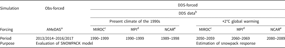
A general modeling procedure to predict the response of snowpack to global warming has been constructed using atmospheric models and a snowpack model. Firstly, a coarse-resolution climate change projection provided by general circulation models (GCMs; Solomon and others, Reference Solomon2007; Stocker and others, Reference Stocker2014) is dynamically downscaled (DDS) into a finer grid for a limited target domain with a 3-D regional climate model (RCM) (Wang and others, Reference Wang2004). Secondly, a 1-D snowpack model is forced with the DDS data at a grid-point location (Rasmus and others, Reference Rasmus, Räisänen and Lehning2004). Snowpack estimation using this procedure strongly depends on the DDS data, which inherently contain uncertainty in the estimation of future climate such as greenhouse gas emission pathway, climate sensitivity in GCMs, planetary-scale circulation in GCMs and local precipitation in GCMs and RCMs. Recently, Katsuyama and others (Reference Katsuyama, Inatsu, Nakamura and Matoba2017) evaluated the response of snowpack to global warming at Kutchan, Shiribeshi, Hokkaido, Japan (Fig. 1a; Table 1), with a clear separation of uncertainty. They used DDS data for a decade (2050–2059, 2060–2069 and 2080–2089 with three different GCM results) when the global mean temperature increased by 2°C relative to present levels (basically 1990–1999 but 1989–1998 with only a GCM) to separate the globally averaged temperature change from the change in synoptic phenomena such as storm tracks, winter monsoons and orographic precipitation (Inatsu and others, Reference Inatsu2015).

Fig. 1. (a) Sub-regions of the island of Hokkaido, Japan names with their abbreviations and color summarized in Table 1. The dotted red rectangle shows the area in (c) and the solid red rectangle in the inset shows the location of Hokkaido in Japan. (b) Altitude (km) of dynamically downscaled (DDS) data. Circles show stations of the Automated Meteorological Data Acquisition System (AMeDAS) where the height of snow cover (HS) is observed. (c) Altitude as in (b) showing snow-pit observation sites (numbered symbols). Symbol color denotes the distance (km) from the nearest AMeDAS station, as given in Table 3. Symbol shape indicates the set of variables observed at the nearest AMeDAS station: star, the full set; hexagon, the set without shortwave radiation; square, the set without shortwave radiation and relative humidity; and triangle, the set without height of snow cover, shortwave radiation or relative humidity.
Table 1. Summary of sub-regions names and their abbreviations in Figures 1a, 10, 11. The color in Figures 1a, 10 is also shown.

The important point in snowpack simulation is to assure model performance via comparison with observation. If only HS were required, the snowpack model could be readily evaluated because HS has been automatically observed at many sites for a long period. However, if other snowpack variables were desired, such as snow water equivalent (SWE) and snow grain types, the lack of observational data would preclude the evaluation of the snowpack model. This is due to the fact that these variables can be obtained only by snow-pit observation, the spatial and temporal resolution of which is insufficient. Probably as a result of this impediment to model evaluation, Bavay and others (Reference Bavay, Grünewald and Lehning2013), who tried to estimate SWE for a relatively wide region, used HS and catchment discharge instead of SWE. Katsuyama and others (Reference Katsuyama, Inatsu, Nakamura and Matoba2017) evaluated the snowpack model for a single target site by comparison with snow-pit observations from a different site far from the target site. Hence, the lack of snow observation is a barrier to performing snowpack estimation over large areas, even though the calculation itself can be accomplished merely by looping the calculation at a single site.
In this study, the approach of Katsuyama and others (Reference Katsuyama, Inatsu, Nakamura and Matoba2017) is expanded to the whole of Hokkaido, Japan (Fig. 1a) by using the same snowpack model and the same DDS dataset, which provided predictions of the characteristics of future snow amount and snow quality. To relieve the problem of the lack of snowpack observations, we use special snow-pit observations from 28 sites over central and eastern Hokkaido during 2014–2017 (Fig. 1c; Shirakawa and Kameda, Reference Shirakawa and Kameda2019). Moreover, we evaluate the model-predicted climatological snow amount by comparison with long-term HS observations from 1990 to 1999 made at 108 stations in Hokkaido operated by the Japan Meteorological Agency (JMA; JMA, 2013). We attempt to evaluate the snowpack model using as much available data as possible to establish the reliability of snowpack estimation forced by DDS data over a large area, Hokkaido, which is characterized with a contrast between much snow amount and predominant rounded grains (RG) in the west and little snow amount and predominant depth hoar in the east (Ishizaka, Reference Ishizaka2008; Shirakawa and Kameda, Reference Shirakawa and Kameda2019).
The remainder of this paper is organized as follows. Section 2 describes the methods of snowpack model evaluation and the estimation of snowpack response to +2°C global warming relative to the present climate (1990–1999) using observational data and DDS data. Additionally, in this section, a simple diagnosis is described which helps us interpret the regional variation and uncertainty of snowpack response to this +2°C global warming. Section 3 provides the results of the snowpack model evaluation and the snowpack response to +2°C global warming. This section also focuses on the uncertainty arising from differences in results among the various boundaries of GCMs for the DDS data. The model evaluation and snowpack response are discussed in Section 4. Finally, Section 5 concludes the paper.
2. Data and method
2.1. Snowpack model
Version 3.3.1 of the SNOWPACK model, a 1-D multi-layered Lagrangian model that basically solves mass- and energy-balance equations via the finite-element method (Bartelt and Lehning, Reference Bartelt and Lehning2002), was used for the snowpack calculations. This model has been used to estimate snowpack behavior at Japanese sites, including in Hokkaido (Hirashima and others, Reference Hirashima, Nishimura, Baba, Hachikubo and Lehning2004; Yamaguchi and others, Reference Yamaguchi, Sato and Lehning2004; Nishimura and others, Reference Nishimura, Baba, Hirashima and Lehning2005; Nakamura and others, Reference Nakamura, Sato, Yamanaka and Nishimura2011; Saito and others, Reference Saito2012; Katsuyama and others, Reference Katsuyama, Inatsu, Nakamura and Matoba2017). The model's metamorphism scheme was set to the NIED option, which included an empirical expression of the metamorphic processes observed in Japan (Hirashima and others, Reference Hirashima, Nishimura, Baba, Hachikubo and Lehning2004). The latent and sensible heat transfer between the snow surface and atmosphere were calculated based on Monin–Obukhov bulk formulation (Michlmayr and others, Reference Michlmayr2008). The output used in this study was the hourly time series of each layer's thickness, density and snow grain type classified into precipitation particles (PP), decomposing and fragmented PP, RG, faceted crystals, depth hoar, surface hoar and MF (Lehning and others, Reference Lehning, Bartelt, Brown, Fierz and Satyawali2002). This study combined PP and decomposing and fragmented PP into a single category (simply called ‘PP’), and also combined faceted crystals, depth hoar and surface hoar into a hoar category (HC). We applied the SNOWPACK model point-by-point on flat terrain, and did not consider the horizontal transport of snow such as snowdrifts and avalanches. These assumptions might not affect the results because the snow transportation has a horizontal scale of 1 km or less, which is much less than the distance between adjacent points in the snowpack calculation (see Section 2.5).
The SNOWPACK model was forced by hourly meteorological data on precipitation, air temperature, relative humidity, wind speed and downward shortwave and longwave radiation. Snowfall should be discriminated from rainfall because the snowpack response to each is quite different (Kudo and others, Reference Kudo, Yoshida and Masumoto2017). Regardless of the dataset, we used the following formula for the fractions of the amount of liquid phase in precipitation:

where T and f, respectively, denote air temperature (°C) and relative humidity (%), T r = 4, T s = 0, $f_{\rm r} = 46\sqrt {7.2-T}$ and f s = −7.5T + 93 (Matsuo and Sasyo, Reference Matsuo and Sasyo1981). The fraction of the solid phase in precipitation is then 1 − w. This discrimination method for solid and liquid precipitation is widely used by meteorologists (e.g. Yasutomi and others, Reference Yasutomi, Hamada and Yatagai2011)
For an accurate calculation of snowpack parameters in a soil-frost environment such as eastern Hokkaido (Hirota and others, Reference Hirota2006), the SNOWPACK model was coupled with a simple soil model containing ten top layers, each with a thickness of 10 cm, five bottom layers, each with a thickness of 20 cm, and a bottommost layer with a thickness of 8 m. The physical properties of the layers were controlled by conductivity, density, heat capacity and volumetric fraction of pores. Because these parameters were completely unknown, we assumed that the bottommost layer of soil was mineral soil and all other layers were a 1:1 mixture of mineral soil and organic soil. Based on a report of the physical properties of mineral and organic soil (Farouki, Reference Farouki1981), the conductivity, density and heat capacity were, respectively, fixed at 2.9 W m−1°C−1, 2650 kg m−3 and 1925 J kg−1°C−1 in the bottommost layer, and at 1.575 W m−1°C−1, 1975 kg m−3 and 2218.5 J kg−1°C−1 in all other layers. For all layers, the volumetric fraction of pores was set to 0.1 (Iwata and others, Reference Iwata2011) and the soil temperature was initially set as the annual mean surface soil temperature at a given point, approximately given by the annual mean air temperature plus 2°C (Hirota and others, Reference Hirota, Fukumoto, Shirooka and Muramatsu1995). The bottom boundary temperature of soil was fixed at the initial temperature since the bottom temperature would be approximately constant with the annual mean surface temperature according to the soil temperature model with our setting of physical soil property (Hirota and others, Reference Hirota, Pomeroy, Granger and Maule2002).
2.2. Snow-pit observation
The snow-pit observations at 28 sites covering the regions of Ishikari and Sorachi, Kamikawa, Tokachi, Okhotsk, and Kushiro and Nemuro (Figs 1a, c) were manually conducted between 2014 and 2017 in late winter (Fig. 2), on dates approximately corresponding to the seasonal maximum of SWE (Shirakawa and Kameda, Reference Shirakawa and Kameda2019). The observed variables were HS, SWE, layer thickness constructing a vertically layered structure of snowpack and the snow grain type of the layer. For the measurement of HS and SWE, three snowpack columns were sampled from the surface to bottom using a Kamuro-type snow sampler with a cross-sectional area of 20 cm2. HS and SWE were then determined by averaging the lengths and weights of the samples. The snow grain type in each layer was subjectively determined by observation of sampled grains with a magnifying glass after digging a snow pit down to the soil–snow interface.
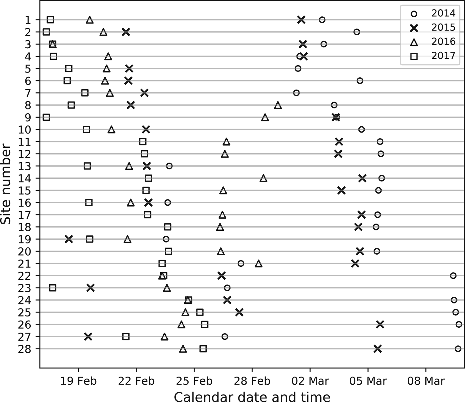
Fig. 2. Local date and time when the snow-pit observations were performed at each site; numbers correspond to those of the sites labeled in Figure 1c. Circles, crosses, triangles and squares, respectively, indicate observation years of 2014, 2015, 2016 and 2017.
2.3. Height of snow cover observations by Automated Meteorological Data Acquisition System
The JMA has operated the Automated Meteorological Data Acquisition System (AMeDAS), a network of ground-based automatic weather stations installed throughout Japan. For the data used in this study, HS observations were operationally conducted via the measurement of the return time of ultrasonic waves or of a laser emitted downwards toward the snow surface. Hourly HS data from 108 sites were used, as shown in Figure 1b. The AMeDAS sites are located in an enough open terrain and flat area with no obstacles near the measurement instruments and satisfy the JMA regulation, so that we can assume that the HS at the site is representative of the value in a local area around the site with little effect of small-scale wind speed.
2.4. Observation-forced simulation
The observation-forced SNOWPACK simulation was performed using hourly atmospheric forcing data observed at 28 AMeDAS stations nearest to the snow-pit observation sites (Fig. 1c, Table 2). Each winter calculation was made from 1 October to the late-winter date when the snow-pit observation was made (Fig. 2). The full set of atmospheric variables observed at the AMeDAS stations were air temperature, precipitation, wind speed and direction, relative humidity, downward shortwave radiation and sunshine duration, meaning that downward longwave radiation was lacking for the SNOWPACK experiment (Section 2.1). Moreover, some AMeDAS stations lacked observations of shortwave radiation (marked as hexagons, squares and triangles in Fig. 1c) and relative humidity (marked as squares and triangles in Fig. 1c). Furthermore, errors in the precipitation observed at AMeDAS stations were sometimes found, with little consistency between precipitation amount and HS increase, despite quality control having already been implemented by the JMA (JMA, 2013). It should be noted that our additional quality control for precipitation observations could not be implemented at the AMeDAS stations where HS was not available (triangles in Fig. 1c). Furthermore, the AMeDAS observation data had some missing values. The aforementioned lacking observations, missing data and errors were complemented with mesoscale analysis data (JMA, 2013) and RADAR-AMeDAS precipitation data (JMA, 2013), with a basis of similarity between AMeDAS data and mesoscale analysis and between AMeDAS data and RADAR-AMeDAS data (not shown). A statistical relationship between the lacking variables and other available variables was also used to estimate the lacking variables. See Appendix A for more details.
Table 2. Summary of the data used and experiments performed in this study.
a Automated Meteorological Data Acquisition System (AMeDAS).
b Dynamically downscaled (DDS) data.
c The high-resolution version of the Model for Interdisciplinary Research on Climate 3.2 (MIROC).
d The fifth-generation atmospheric GCM of the Max Planck Institute for Meteorology, Hamburg, Germany (ECHAM5/MPI).
e Version 3 of the Community Climate System Model of the US National Center for Atmospheric Research (CCSM3/NCAR).
Table 3. Positions of snow-pit observations and their nearest AMeDAS station.
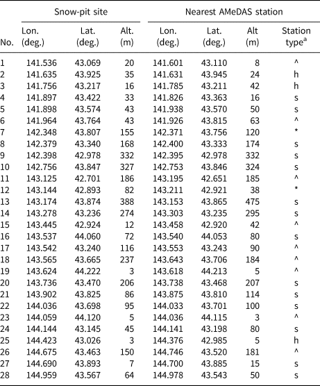
a Symbols in the rightmost column indicate the AMeDAS observation variables: an asterisk (star marks in Fig. 1c) denotes the full set of variables to run the SNOWPACK model except for downward longwave radiation; ‘h’ (hexagons in Fig. 1c) denotes the additional lack of shortwave radiation; ‘s’ (squares in Fig. 1c) denotes the additional lack of relative humidity; and hat (‘^’) (triangles in Fig. 1c) denotes the additional lack of height of snow cover.
2.5. DDS-forced simulation
The DDS-forced SNOWPACK simulation was performed with hourly DDS data under the present climate of the 1990s and +2°C global warming at all longitude–latitude grid points in Hokkaido (Table 2). The calculation ran from 1 October to 31 August of the following year. The DDS provided all the atmospheric variables necessary to drive the SNOWPACK model, but the DDS data originally had a systematic bias. The air temperature and precipitation were bias-corrected by comparing climatic observations with the 10-year mean of the DDS data under the present climate, since the estimation of snowpack parameters was quite sensitive to air temperature and precipitation (López-Moreno and others, Reference López-Moreno, Pomeroy, Revuelto and Vicente-Serrano2013). The DDS temperatures were simply offset for the monthly mean to match with the MESHCLIM 2010 climate mesh (Kitamura, Reference Kitamura1990) provided by the JMA. In this procedure, a MESHCLIM grid configuration with a 1 km spacing was aggregated into the DDS grid configuration with a 10 km spacing. The DDS precipitation was simply multiplied by a correction coefficient (Prudhomme and others, Reference Prudhomme, Reynard and Crooks2002) for the monthly climate data to match with the monthly climate data of the APHRO_JP gridded precipitation data (Kamiguchi and others, Reference Kamiguchi2010) after APHRO_JP data were re-gridded into the DDS grid configuration. A bias correction was not performed for wind speed, shortwave radiation or relative humidity, but downward longwave radiation was replaced with a statistically estimated value obtained from relative humidity and bias-corrected air temperature, following Kondo and others (Reference Kondo, Nakamura and Yamazaki1991) (Hirashima and others, Reference Hirashima, Nishimura, Yamaguchi, Sato and Lehning2008), due to the strong dependence of longwave radiation on temperature.
The atmospheric forcing was prescribed as each of three DDS datasets with the numerical integration of the JMA/Meteorological Research Institute non-hydrostatic model (Saito and others, Reference Saito2006) with a 10 km horizontal resolution imposed with different lateral boundaries of the high-resolution version of the Model for Interdisciplinary Research on Climate 3.2 (MIROC; Hasumi and Emori, Reference Hasumi and Emori2004), the fifth-generation atmospheric GCM of the Max Planck Institute for Meteorology, Hamburg, Germany (ECHAM5/MPI; Roeckner and others, Reference Roeckner2003), and version 3 of the Community Climate System Model of the US National Center for Atmospheric Research (CCSM3/NCAR; Collins and others, Reference Collins2006), all of which contributed to the Coupled Model Inter-Comparison Project Phase 3 (CMIP3) (Kuno and Inatsu, Reference Kuno and Inatsu2014). These three GCMs were comparably reliable in the reproduction of the atmospheric circulation around Japan under the present climate in winter (Kuno and Inatsu, Reference Kuno and Inatsu2014) and in summer (Inatsu and others, Reference Inatsu2015). The present-climate DDS data were created using MIROC results for 1990–1999, MPI results for 1990–1999 and NCAR results for 1989–1998. The future-climate DDS data were created using MIROC results for 2050–2059, MPI results for 2060–2069 and NCAR results for 2080–2089, each of which corresponds to a decade when the global mean air temperature was predicted to increase by 2°C relative to present levels in the Special Report on Emissions Scenarios A1b (Solomon and others, Reference Solomon2007). These decades with a +2°C global warming enabled us to evaluate the uncertainty in synoptic phenomena that are independent of climate sensitivity and emission amount (Section 1; Inatsu and others, Reference Inatsu2015). It should be noted that the 10-year mean (1990–1999) and 20-year mean (1980–1999) were nearly the same (Inatsu and others, Reference Inatsu2015), although the 10-year mean was considered too short to compute a climatological value. See Kuno and Inatsu (Reference Kuno and Inatsu2014) for more details of the DDS calculation.
Figure 3 shows the bias-corrected climatological air temperature for Hokkaido (10-year mean) for December, January and February (DJF), and its response to the +2°C climate. The temperature in the region in these months ranges from −10 to 0°C in the present climate, being warmer in the Oshima and Hiyama sub-region and colder in the Rumoi and Soya, Kamikawa, and Okhotsk sub-regions (Figs 1a, 3a). The global warming response showed a significant increase of 2–4°C in Hokkaido (Figs 3b–d). Using the DDS with the NCAR GCM, a greater temperature increase was predicted in the Rumoi and Soya, Okhotsk, Kushiro and Nemuro, and Tokachi sub-regions (Fig. 1a), while using the DDS with the MIROC and MPI GCMs, a more uniform increase was predicted across Hokkaido. The large increase with NCAR would be highly sensitive to an ablation of sea ice which made the temperature warmer through ice-albedo feedback and stronger monsoonal northwesterly (Matsumura and Sato, Reference Matsumura and Sato2011). Figure 4 shows the bias-corrected climatological precipitation (also a 10-year mean) for DJF and its response to the +2°C climate. In the present climate, high precipitation is observed along the Sea of Japan coast, while less precipitation is observed along the other coasts (Fig. 4a). The DDS results for the +2°C climate showed an increase in precipitation in Hokkaido (Figs 4b–d) due to the Clausius–Clapeyron relation. Precipitation on the western side of the central mountains, anti-correlated with the storm track activity passing south of Japan (Nakamura, Reference Nakamura1992), significantly increased in the DDS using the MIROC and MPI boundaries, and increased uniformly in the DDS using the NCAR boundary. This feature is consistent with the stronger storm track activity responding to the global warming with MIROC boundary (Inatsu and Kimoto, Reference Inatsu and Kimoto2005). The increase in Rumoi and Kamikawa and Kamikawa sub-regions would be partially related to the changes in monsoonal northwesterly with NCAR boundary (Matsumura and Sato, Reference Matsumura and Sato2011).
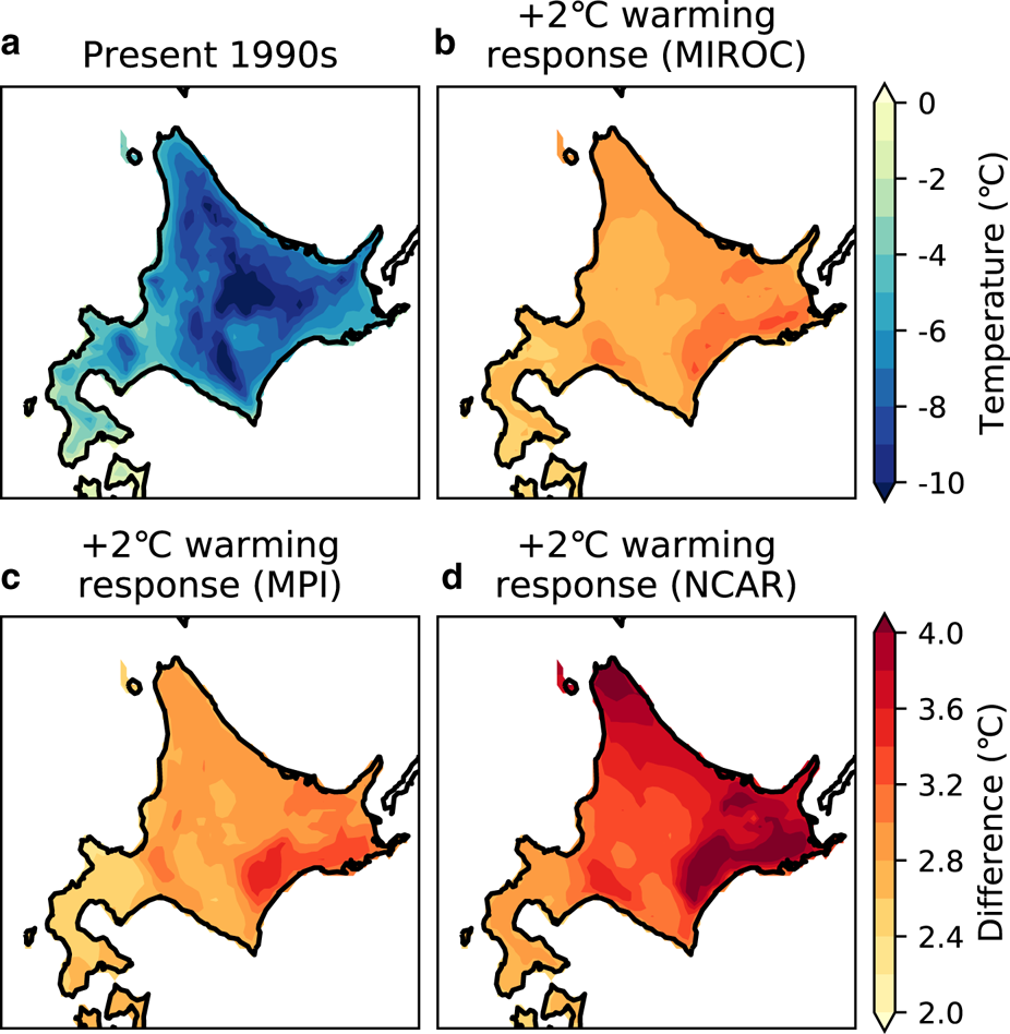
Fig. 3. (a) Bias-corrected 10-year mean air temperature from the DDS data from December, January and February (DJF) in the present climate and its difference with the temperatures predicted for the +2°C global warming climate scenario using the DDS data of the boundary conditions of (b) MIROC, (c) MPI and (d) NCAR.

Fig. 4. (a) Bias-corrected 10-year mean daily precipitation in DJF in the present climate and its difference with the precipitation predicted for the +2°C global warming climate scenario using the DDS of the boundary conditions of (b) MIROC, (c) MPI and (d) NCAR. The hatched areas denote statistical significance at the 5% level.
2.6. Diagnosis of direct and indirect temperature response
We separated the pure direct effect of a rising temperature baseline corresponding to a global warming level from other effects. Following Casola and others (Reference Casola2009), a relative increase in SWE is expressed as the sum of the direct effect and the residual:

where T and Q are the climatological air temperature and seasonal-maximum SWE, respectively, and δT is the global mean temperature increase, which is 2°C in this study. The residual δQ′/Q is now called the indirect effect, and includes the uncertainty across the GCM boundaries and other effects, such as the change in precipitation that accompanies the rise in global mean temperature. Therefore, the indirect effect with MIROC and NCAR boundaries may be different with MPI boundary in some sub-regions responding to the stronger storm activity and winter monsoon (Section 2.5). In contrast, the direct effect includes only the pure direct effect of a rise in temperature baseline of 2°C. The direct effect does not depend on the GCM projection, but rather only on the relative sensitivity of the seasonal-maximum SWE (1/Q)(dQ/dT) depending on sub-regions, which is always negative because the snow amount must decrease by the temperature increase. We obtained this relative sensitivity based on the scatter plot of point-by-point climatological air temperatures and seasonal-maximum SWEs in each sub-region under the present 1990s climate, which reflects the effect of topographic height to sensitivity. The indirect effect is then obtained by subtracting the direct effect from the total change δQ/Q estimated based on the comparison of DDS simulation between the present 1990s climate and the +2°C climate.
3. Results
3.1. Model evaluation
The SNOWPACK model was first evaluated by a comparison of values of HS, SWE and the thickness ratio of RG, MF and HC on a late-winter date obtained by the observation-forced simulation with values obtained from AMeDAS atmospheric data (Section 2.4) and special snow-pit observations at 28 sites (Section 2.2). This evaluation revealed that the SNOWPACK model moderately reproduced HS and SWE on a late-winter date at the 28 snow-pit sites, with relative errors mostly <50% (Fig. 5). With the metric of thickness ratio defined as the ratio of the time-integrated layer thickness of a particular snow grain type to the time-integrated thickness of the whole snowpack, RG was well reproduced in Hokkaido, while MF was underestimated and HC was overestimated at some sites in the Ishikari and Sorachi and Kamikawa sub-regions (Fig. 6).
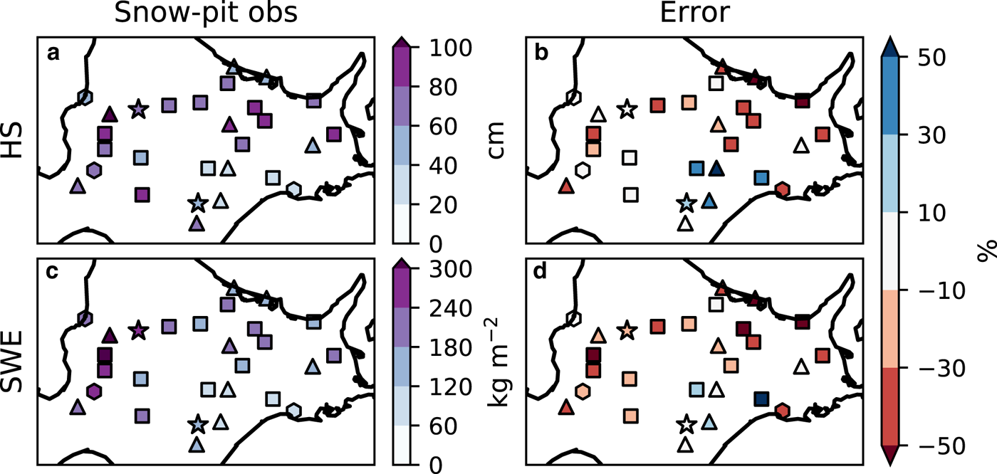
Fig. 5. A comparison between data from snow-pit observations and those from the observation-forced simulation. (a) Observed mean height of snow (HS), (b) mean error of the calculated HS, (c) observed mean snow water equivalent (SWE) and (d) mean error of the calculated SWE.
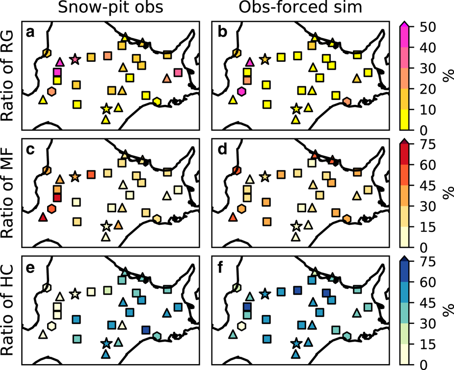
Fig. 6. Mean thickness ratio of (a) rounded grain (RG), (c) melt form (MF) and (e) hoar category (HC) obtained by snow-pit observation. The figures (b, d, f): same as (a, c, e), but for the observation-forced simulation.
Next, the SNOWPACK model was evaluated by a comparison between the seasonal-maximum HS and the number of snow-covered days (SCDs), which is here defined as the total number of days with a daily maximum HS larger than 5 cm, obtained from the DDS-forced simulation under the present climate (Section 2.5), and the values obtained by routine AMeDAS observation at 108 stations in Hokkaido (Section 2.3). Although biases without monthly mean air temperature and monthly mean precipitation probably remained in the bias-corrected DDS data, that are strictly different data among the GCM boundaries, the DDS-forced simulation of all GCM boundaries commonly showed that the seasonal-maximum HS reached 150 cm along the coast of the Sea of Japan due to moisture advection by the winter monsoon (Figs 4a, 7a–c), and the SCDs mostly ranged from 100 to 200 d due to low temperatures (Figs 3a, 7d–f). It was noted that the seasonal-maximum SWE showed a similar distribution to the HS, however this parameter was not used in the model evaluation because seasonal-maximum SWE was not measured at AMeDAS stations (Figs 7g–i). Comparison with the AMeDAS observations revealed only a few stations with an underestimation of HS of more than 50% (Figs 7a–c), and a few stations with an overestimation of SCDs of more than 30 d (Figs 7d–f).
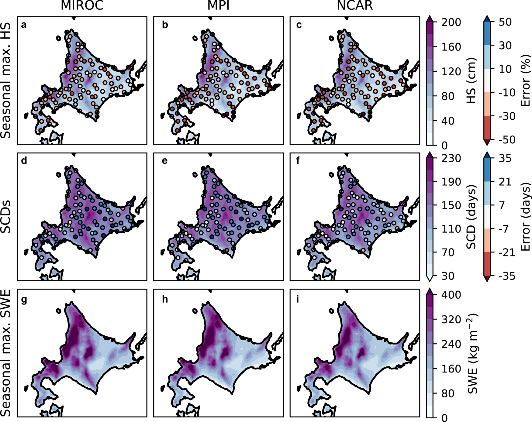
Fig. 7. The 10-year mean of: (a–c) seasonal-maximum HS and its error based on AMeDAS observation; (d–f) snow-covered days (SCDs) and its error from the AMeDAS observation; and (g–i) seasonal-maximum SWE obtained by the DDS-forced simulation of the boundary conditions of (a, d, g) MIROC, (b, e, h) MPI and (c, f, i) NCAR, in the present climate. The errors in HS are normalized by the observation with the rightmost color scale.
In the model evaluation, the results of the observation-forced simulation and the DDS-forced simulation under the present climate were separately compared with the observations. These two different comparisons were achieved using a Taylor diagram displaying the spatial correlation, Std dev. and root-mean-square error (RMSE) (Taylor, Reference Taylor2001; Fig. 8). Note that the Std dev. and RMSEs of the simulations were normalized by the Std dev. of the observations. In the Taylor diagram, the performance of the model was generally judged by how close a simulation point was to the reference point cross-marked at (1, 0) (Fig. 8). According to the diagram, the climatology of seasonal-maximum HS was best reproduced by the SNOWPACK model, with a spatial correlation of 0.9 and an RMSE of 0.5 relative to the Std dev. of the observed data. The climatology of SCDs was also well reproduced with slightly worse scores than the case of seasonal-maximum HS. Whereas the snow amount at a specific time by the observation-forced simulation was worse than the climatology by the DDS-forced simulation, HS was better reproduced than SWE focusing only on the observation-forced simulation. This might indicate a better production of the climatology of seasonal-maximum SWE than that of seasonal-maximum HS because of linearity between SWE and HS (Shirakawa and Kameda, Reference Shirakawa and Kameda2019).
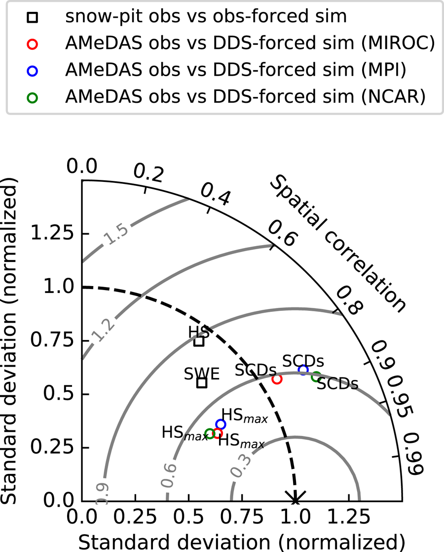
Fig. 8. Taylor diagram showing the comparison between simulated and observed parameters. Black squares show the comparison between the HS and SWE values obtained by snow-pit observation and those obtained by observation-forced simulation. Colored circles show comparisons between the seasonal-maximum HS (HSmax) and the snow-covered days (SCDs) obtained from AMeDAS observations and those obtained from the DDS-forced simulation in the present climate. Red, blue and green denote the boundary conditions of MIROC, MPI and NCAR, respectively. The Std dev. and the root mean square errors (RMSEs) of the simulations are normalized by the Std dev. of the observations. Concentric gray lines centered on the reference point (indicated by a cross mark) show RMSE.
3.2. Response to +2°C global warming
Figure 9 shows the response of the seasonal-maximum HS and SWE, and SCDs, to the +2°C global warming climate scenario. The SNOWPACK simulation driven by the DDS data with any GCM boundaries commonly predicted significantly decreased HS (by 30%) and SWE (by 40%) in the Oshima and Hiyama, Shiribeshi, and Iburi and Hidaka sub-regions, probably due to a significant increase in temperatures throughout the winter season (Fig. 3). In the Kushiro and Nemuro sub-region, the predicted HS and SWE also decrease, exceeding a 5% statistical significance level regardless of the choice of GCM boundaries, except for the decrease of HS for the MIROC and MPI boundaries, which were not statistically significant. Under the +2°C global warming, the number of SCDs in Hokkaido commonly declined by ~30 d with a statistically significant level at 5%. This shortening indicates, for example, that the +2°C climate would result in only half as many SCDs in the Oshima and Hiyama and the Kushiro and Nemuro sub-regions compared with the present climate. Focusing on a variety of results across the GCM boundaries imposed on DDS, the uncertainties in HS and SWE were quite large in the Rumoi and Soya sub-region (Fig. 1a); a significant decrease in HS (by 20%) was predicted only for MPI and an insignificant decrease in SWE was predicted only for NCAR. The snowpack response in terms of HS and SWE significantly depended on elevation; the HS and SWE were predicted to decrease slightly on the highest mountain located at the boundary between the Kamikawa and Tokachi sub-regions, while the HS and SWE were predicted to decrease by 30–40% in the Ishikari and Sorachi sub-region in a flat plain (Figs 1, 9). This dependency on elevation is consistent with previous studies (e.g. Kawase and others, Reference Kawase2013; Katsuyama and others, Reference Katsuyama, Inatsu, Nakamura and Matoba2017).
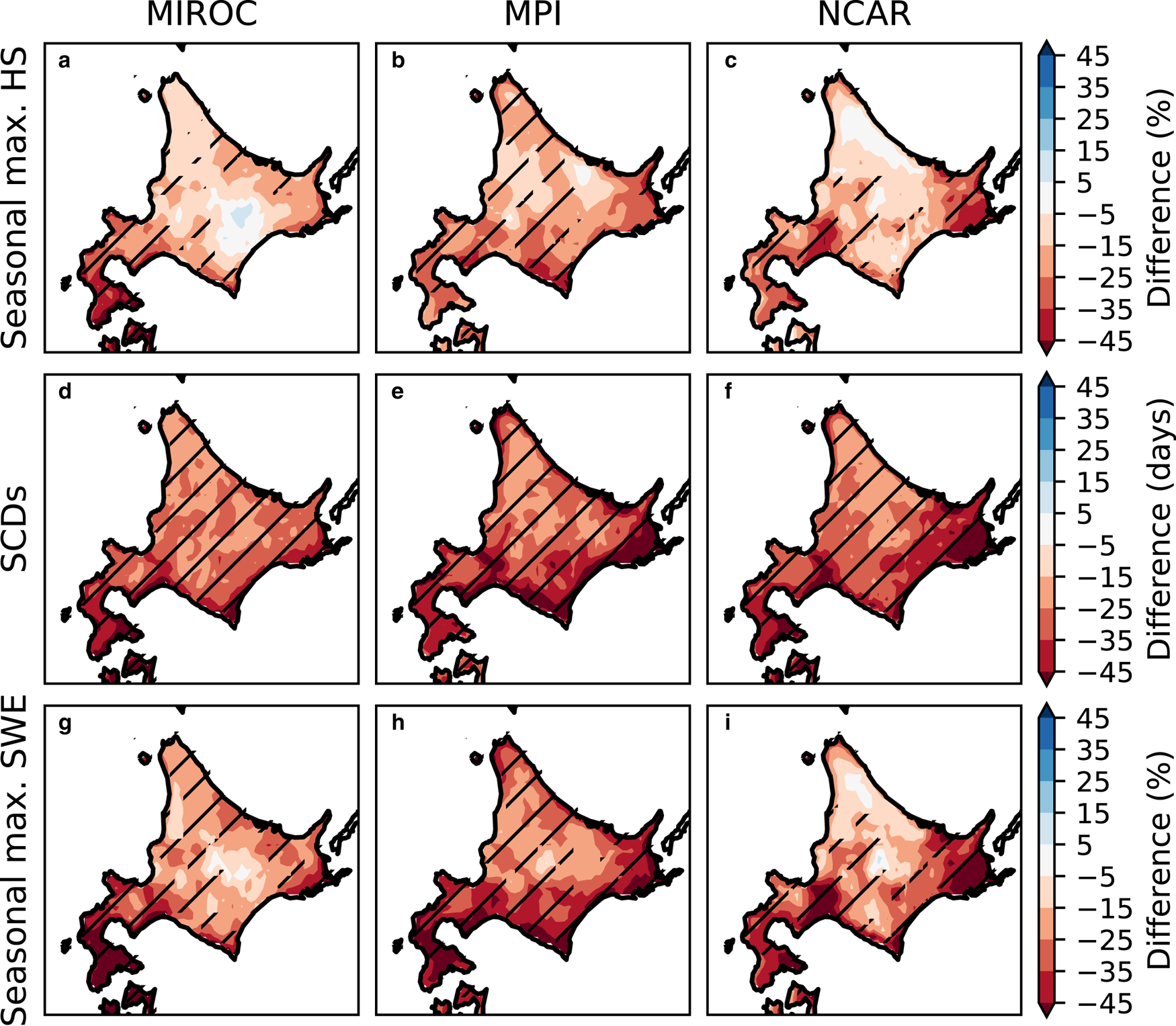
Fig. 9. The difference in the 10-year mean of (a–c) seasonal-maximum HS, (d–f) SCDs and (g–i) seasonal-maximum SWE, between the +2°C global warming climate scenario and the present climate. The difference between HS and SWE is normalized by the present climate. The hatched areas show statistical significance at the 5% level.
Moreover, we investigated the decrease in the seasonal-maximum snow amount and its uncertainty among GCM boundaries using Eqn (2) for each sub-region (Fig. 1a). Figure 10 shows a scatter plot of air temperature in DJF (Fig. 3a) approximately covering the snow accumulation period versus the seasonal-maximum SWE (Figs 7g–i) for all GCM boundaries for all grid points in each sub-region under the present climate. By linear fitting of the scattered data, the sensitivity of SWE to temperature ((1/Q)(dQ/dT) in Eqn 2) was determined to range from −14 to −3%°C−1 (Fig. 10), which is nearly consistent with previous studies focusing on Western North America (Casola and others, Reference Casola2009) and Japanese main island, Honshu (Kawase and others, Reference Kawase2013). The sensitivity of SWE to temperature was statistically stable, with a narrow confidence interval of 95% in all sub-regions (not shown).
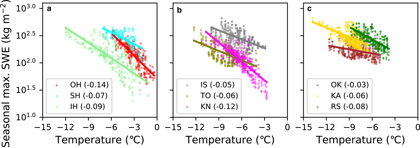
Fig. 10. Scatterplots of the 10-year mean of seasonal-maximum SWE versus the 10-year mean of air temperature in DJF under the present climate for all the DDS grid points in the (a) OH, SH and IH sub-regions; (b) IS, TO and KN sub-regions; and (c) OK, KA and RS sub-regions. Colors as in Figure 1a/Table 1. The best-fitting line is superimposed for each dataset, with its slope ((1/Q)(dQ/dT) in Eqn 2) given in the legend.
By multiplying the 2°C increase in global mean temperature (δT = 2) by the estimated temperature sensitivity of SWE ((1/Q)(dQ/dT); Fig. 10), it was found that the 2°C increase would directly decrease SWE by 6–28%; this is referred to as the direct effect (Eqn 2; Fig. 11). This direct effect was strongest in the Oshima and Hiyama, Kushiro and Nemuro, and Rumoi and Soya sub-regions (Figs 11a, f, i). Additionally, the indirect effects (δQ′/Q) were also calculated as by subtracting the direct effects from the total (Eqn 2; Fig. 11). The indirect effect for SWE was larger than the direct effect in the Shiribeshi, Ishikari and Sorachi, and Okhotsk sub-regions for all the DDS-forced simulations, which means that the indirect effect provided the major contribution to the total decrease in SWE. In these sub-regions, the variation in the indirect effect among GCM boundaries was quite small. In contrast, the indirect effect of only the MPI boundary caused the major contribution to the total decrease in SWE, while the indirect effects of the other boundaries did not cause the major contribution in the Iburi and Hidaka, Tokachi, Kamikawa, and Rumoi and Soya sub-regions. This was well consistent with what the MPI was a case of less obvious atmospheric response to the global warming such as changes in storm track and winter monsoon than the MIROC and NCAR (Fig. 4; Section 2.5).

Fig. 11. The difference between the +2°C global warming climate scenario and the present climate for seasonal-maximum SWE, precipitation and runoff amount integrated during the accumulation period, averaged over each sub-region. The direct and indirect effects of the difference in seasonal-maximum SWE are also shown. Red, green and blue colors indicate the boundaries of MIROC, MPI and NCAR.
The total decrease in seasonal-maximum SWE was split into that of the total amounts of precipitation (P), runoff (R) and evaporation and sublimation (E) integrated during the accumulation period, defined from an initial snow-covering date to the date of seasonal-maximum SWE, based on the modeled mass conservation expressed as Q = P − R − E. Because evaporation and sublimation were quite small (not shown), the sum of decreases in the precipitation and runoff was nearly equal to the total decrease in SWE, that is δQ ≈ δP − δR. These integrated amounts are controlled by the air temperature (Fig. 3a), the daily amount of precipitation (Fig. 4a) and shortening of snowfall season which in turn is SCDs (Figs 7d–f). Figure 11 shows that the change in the integrated precipitation was the main contributor to the total SWE decrease in most of the sub-regions. In Oshima and Hiyama, Tokachi, Kushiro and Nemuro, and Okhotsk sub-regions where the daily amount of precipitation would not significantly change due to uncertain atmospheric changes (Fig. 4), the decrease in the integrated precipitation was much large. This feature was predicted even in the other sub-regions where the daily amount of precipitation would significantly increase (Figs 4, 11), though the decrease in the integrated precipitation would be less (Fig. 11). Therefore, the decrease in the integrated precipitation here is mainly attributed to the decrease in the number of SCDs (Fig. 9). However, the increase in runoff is predicted to contribute as much to the total SWE decrease as the precipitation decrease in the Ishikari and Sorachi, Kamikawa, and Rumoi and Soya sub-regions (Figs 11d, h, i), even though the runoff should be predicted to decrease following the decline in the number of SCDs if the daily amount of runoff did not increase. The variations of changes in the integrated precipitation and runoff amounts across GCMs are also controlled by that in the air temperature, daily amount of precipitation and SCDs. Then, the decrease in the integrated precipitation would be much large with MPI in Iburi and Hidaka sub-region, which was a case of less obvious atmospheric response to the global warming such as changes in storm track and winter monsoon (Fig. 4; Section 2.5). This feature was recognized in the other sub-regions, and the decrease in the integrated precipitation would be mostly uncertain (Fig. 11). On the other hand, the increase in runoff amount integrated over the accumulation period would be fairly certain in most sub-regions (Fig. 11). Since the decrease in SCDs was not uncertain (Figs 9d–f), it is thought that the uncertainty in the seasonal-maximum SWE decrease is mainly attributed to the uncertainty in the daily precipitation change related to the atmospheric response.
Figures 12 and 13 show the response to global warming of the total thickness ratio of PP, RG, MF and HC for whole winter seasons. Considering the bias in the SNOWPACK model (Section 3.1), we only showed the climatological thickness ratio averaged over all DDS results weighted by the time-integrated thickness of the whole snowpack for each DDS result. The ratio of PP is predicted to increase in the Oshima and Hiyama and Ishikari and Sorachi sub-regions in the +2°C climate scenario relative to the present climate (Figs 12a, b), even though the temperature is predicted to increase (Fig. 3). While the ratio of RG is predicted to tend to decrease (Figs 12c, d), that of MF is predicted to tend to increase. MF is predicted to occupy more than half of the snow amount in the Shiribeshi, Iburi and Hidaka, and Kushiro and Nemuro sub-regions in the +2°C climate scenario (Figs 13a, b). In contrast, the ratio of MF is predicted to decrease by 30–40% in the Oshima and Hiyama sub-region, where MF is predicted to exceed that of the present climate by 50%. This indicates that the density of the total snow cover will be lower, because PP is lighter than MF. The HC-dominated area is predicted to almost completely vanish in the +2°C climate scenario, while HC was the dominant snow grain type in the Okhotsk and Tokachi sub-regions under the present climate due to the low temperature and low precipitation (Figs 13c, d). The decrease in the HC-dominated area is consistent with a rough statistical estimation made in previous studies (Inoue and Yokoyama, Reference Inoue and Yokoyama2003), in spite of the moderate model bias in MF and HC (Section 3.1).

Fig. 12. (a, b) The total thickness ratio of precipitation particles (PP) under (a) the present climate and (b) the +2°C global warming climate scenario predicted by the DDS-forced simulation. (c, d) Same as (a, b), but for RG.
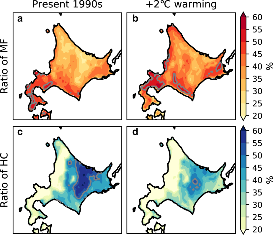
Fig. 13. (a, b) The thickness ratio of MF under (a) the present climate and (b) the +2°C global warming climate scenario predicted by the DDS-forced simulation. (c, d) Same as (a, b), but for HC. The gray contour indicates a ratio of 50%.
4. Discussion
4.1. Model evaluation
We evaluated the SNOWPACK model by comparing the results of the observation-forced simulation with the snow-pit observations. There is a potential concern about the representativeness of snow-pit sites, especially in mountainous regions in which the snowpack state is not always the same as the dominant state in the surrounding area. First, observation sites were selected, with all efforts made to exclude non-standard sites such as those with buildings nearby, those on top of a hill, those at the bottom of a valley, those in the center of a town or those with restricted access. The sites were generally located in homogeneous areas, without any buildings nearby. A pair of sites, #18 and #20, which are located near one another in a mountainous region (Fig. 1c), and for which observations were made at almost at the same times (Fig. 2), showed very similar observed snowpack states (Figs 5a, c, 6a, c, e). Additionally, almost simultaneous observations at sites #11 and #12 (Figs 1c, 2) also showed a similar snowpack states (Figs 5a, c, 6a, c, e). These results support the supposition that the snow-pit observations well reflected the typical snowpack state around the sites.
In the observation-forced simulation, the forcing data were assumed to be unbiased; however, MF was underestimated and HC was overestimated at some sites in the Ishikari and Sorachi and Kamikawa sub-regions (Figs 6a–d). In addition, the snowpack amount at a few sites, #5, #21, #23 and #27, were largely underestimated by over 50% (Fig. 5). There are three possibilities relating to forcing data that might lead to a bias in the snowpack simulation. The first possibility for the bias is the lack of observation of some variables at AMeDAS sites, which are complemented with statistical estimation or replaced with analytical data from the nearest gridpoint (Section 2.4). In particular, the precipitation remained biased at some sites with no HS observation. However, the error in HS, SWE and snow grain type has no significant dependence on the extent of the lack of observational variables (Figs 5, 6). The second possibility for the error is distance between AMeDAS stations and snow-pit sites (Fig. 1c). However, the results suggest that the systematic error was insensitive to this distance (Figs 5, 6). Hence, we consider that the error in the observation-forced simulation is not basically caused by meteorological input, though imperfect quality control on precipitation data was still concerned at #23 and #27, where precipitation frequently accompanied strong wind over 10 m s−1 (not shown). The third possibility for the bias is the representativeness of snow observation due to site-scale wind distribution. In an ideal sense, it might be said that the HS data were affected by the buildings and trees around the site, if any. Moreover, the blowing snow due to strong wind could accumulate or erode site-scale snow and then affect site-scale HS distribution. Such pessimistic ideas never wipe out completely without dense and perfect observation. Yet, a moderate consistency between observation and simulation in most of 108 points (Figs 7a–c, 8) reversely assured the representativeness of AMeDAS observation not in a sense of an individual site but as an overall evaluation for sites over Hokkaido.
We furthermore discuss the bias in snow grain types of the SNOWPACK model that successfully reproduced the SWE. The tendency to overestimate HC is possibly due to an unreasonable growth rate of sphericity and/or an overestimation of the snowpack temperature gradient (Bartelt and Lehning, Reference Bartelt and Lehning2002; Hirashima and others, Reference Hirashima, Nishimura, Baba, Hachikubo and Lehning2004). The unreasonable growth rate of sphericity would only lead to a bias in HC because the growth rate is a snowpack microstructural parameter of metamorphosis efficiency (Lehning and others, Reference Lehning, Bartelt, Brown, Fierz and Satyawali2002). The overestimation of the snowpack temperature gradient would also lead to a bias in HS because the temperature gradient might affect the snowpack settlement (Bartelt and Lehning, Reference Bartelt and Lehning2002). However, the DDS-forced simulation did not show a bias in the seasonal-maximum HS in the present climate (Fig. 8). Therefore, we consider that the unreasonable growth rate might bias HC, and the thickness ratio of the other grain types was biased to keep the sum of ratios unity. If one desired to improve the estimate of HC amount in the SNOWPACK calculation, it might be possible to set a different value of the growth rate of sphericity for each sub-region. However, we have still given this parameter uniformly over Hokkaido to maintain consistency in the physics of snow metamorphosis.
In the DDS-forced simulation, the SNOWPACK model was forced by the DDS results from the MIROC and the GCMs of MPI and NCAR with a single RCM (Kuno and Inatsu, Reference Kuno and Inatsu2014). These GCMs were selected by Kuno and Inatsu (Reference Kuno and Inatsu2014) because the models reasonably reproduced atmospheric circulation around Japan under the present climate. We corrected the systematic DDS bias in temperature and precipitation, which is quite important for snowpack calculation (López-Moreno and others, Reference López-Moreno, Pomeroy, Revuelto and Vicente-Serrano2013) (Section 2.5). If the forcing data had biases in other variables, such as radiation, the data should have different features among the GCM boundaries. However, the results of the DDS-forced simulation were not largely different between the different GCM boundaries (Fig. 7).
Comparing the results between the observation-forced and DDS-forced simulation, snowpack amount at a specific date and time was worse reproduced than the climatology of that (Fig. 8), including large error in SWE at #23 and #27 snow-pit sites. However, we focused on the climatology of snowpack over Hokkaido in this study, so that the best reproduction of climatology of seasonal-maximum HS (Fig. 8) strongly supported an ability that SNOWPACK could be applied to the climate modeling. Fortunately, in the observation-forced simulation, SWE had been better reproduced than HS, the best reproduction in climatological time-scale. We had also discarded sites #23 and 27 in tuning SNOWPACK model because it is unreasonable to tune the model site by site considering that the model must follow the physical laws.
We performed the snowpack calculation gridpoint by gridpoint, assuming that a single gridcell is sufficient in an open terrain and that a gridpoint is representative of the surrounding environment (Section 3.2). However, a realistic gridcell contains more complex terrain and varied vegetation. For example, snow is largely redistributed in mountainous regions, and then the thinner snowpack rapidly diminishes in the snow melting season. This makes it difficult to compare snowpack observations with our calculations. A combination of higher-resolution atmospheric forcing data and a physical snowpack and snow transport models (e.g. Lehning and others, Reference Lehning2006) may resolve the problem, albeit with a greatly increased computational cost.
4.2. Snowpack response to +2°C global warming
We investigated the decrease in the seasonal-maximum SWE based on the climate sensitivity to air temperature (Figs 10, 11). Then, the direct effect would be the major contributor to the total decrease, so that the regional variation of the sensitivity of seasonal-maximum SWE to the climatology of air temperature would be the major causality to the decrease in SWE depending on sub-regions (Fig. 11). One reason for the regional variation of sensitivity was air temperature during the accumulation period when precipitation occurred; the sensitivity would be high if the precipitation occurred around in the freezing point of air temperature. Another reason was related to a temperature profile of inner snowpack. If the snowpack was isothermal condition in vertical, snowpack would immediately start to melt above the freezing point. Since warm condition in air temperature often coincided with strong incoming shortwave radiation, the radiation furthermore promoted the snowpack melting (López-Moreno and others, Reference López-Moreno, Pomeroy, Revuelto and Vicente-Serrano2013). The isothermal condition is roughly diagnosed by the thickness ratio of MF (Lehning and others, Reference Lehning, Bartelt, Brown, Fierz and Satyawali2002). In Oshima and Hiyama sub-region (Fig. 1a), where MF were dominant (Fig. 13a) and much snowfall was given around in the freezing point (not shown), therefore, the sensitivity to air temperature was much high (Fig. 10a). On the other hand, in Okhotsk sub-region (Fig. 1a), where MF were merely formed (Fig. 13a) and much snowfall was produced in enough cold air temperature (not shown), the sensitivity was much low (Fig. 10c).
The estimate at the fixed 2°C warming can be extended to any future time in any scenario, if the analysis is limited to the direct effect, with the use of the sensitivity of SWE to air temperature (Fig. 10). For example, the RCP8.5 scenario with the new-generation CMIP5 models (Moss and others, Reference Moss2010) provided a global air temperature increase of 2°C in the 2050s and of 4°C in the 2100s relative to the 1990s temperature (Stocker and others, Reference Stocker2014). The direct effect would then be double (1/Q)(dQ/dT) in the 2050s and quadruple (1/Q)(dQ/dT) in the 2100s (Eqn 2; Fig. 10). In the Oshima and Hiyama sub-region, the direct effect is predicted to lead to a decrease in SWE of 28% in the 2050s (Fig. 10a). Similarly, the RCP2.6 scenario saturated the temperature increase at 1°C after the 2050s (Stocker and others, Reference Stocker2014). The direct effect would explain the SWE decrease saturating at a value of (1/Q)(dQ/dT). Similarly, the uncertainty in the SWE decrease due to the direct effect would be also estimated as 3–14% in the 2050s under the RCP8.5 scenario among 39 GCMs, where the global mean temperature increases ranged between 1.5 and 2.5°C (Stocker and others, Reference Stocker2014). However, we could not estimate the total decrease in seasonal-maximum SWE due to the large uncertainty in the indirect effect. A large number of GCMs would be needed to evaluate this uncertainty accurately, however this study considered only three GCMs.
As a similar context of our interpretation on the decrease in SWE based on the sensitivity to air temperature, the shortening number of SCDs predicted in this study was interestingly reviewed by Hantel and others (Reference Hantel, Ehrendorfer and Haslinger2000), who explained SCD normalized by a reference SCD based on a sigmoid model. In their model, the sensitivity of the SCD to temperature was zero in a fully snow-covered or non-snow-covered case, whereas it was a negative maximum in a case where the normalized SCD is 50%. Our analysis showed that SCDs in the Oshima and Hiyama and Kushiro and Nemuro sub-regions would significantly decrease by ~50% under the +2°C global warming climate scenario regardless of the choice of GCM boundaries (Figs 7g–i, 9g–i). This actually corresponded to the negative maximum sensitivity of SCDs, so that the uncertainty of decrease was expected to be strongly affected by that of an increase in air temperature. However, the uncertainty would not be large (Figs 9g–i) due to small uncertainty of increase in air temperature (Figs 3b–d). On the other hand, in Kushiro and Nemuro where the 50% decrease in SCDs (Figs 9d–f) and large uncertainty of increase in air temperature (Fig. 3) were also estimated, the uncertainty of decrease in SCDs would be large due to the strongest sensitivity of SCDs. Interestingly, in Rumoi and Soya where the large uncertainty of increase in air temperature was estimated as well as Kushiro and Nemuro, the uncertainty of decrease in SCDs was much small because the decrease in SCDs was not sensitive to air temperature due to small decrease in SCDs.
5. Conclusion
We have performed two experiments: observation-forced simulation for 28 sites in Hokkaido in the winters of 2013/14 to 2016/17, and DDS-forced simulation at all the grid points in Hokkaido for ten winters of the present climate (1990–1999) and for a +2°C global warming climate scenario relative to the present level using three GCM boundaries selected from CMIP3 models with the A1b scenario (Table 2). The comparison of HS, SWE and the ratios of MF, RG and HC obtained by the observation-forced simulation and those obtained from the special snow-pit observations were used to evaluate the snowpack model, even with the moderate bias that the model underestimated the MF and overestimated the HC in the Ishikari and Sorachi and Kamikawa sub-regions (Figs 5, 6). Moreover, SCDs and seasonal-maximum HS were evaluated by comparing the results of the DDS-forced simulation with the operational observations of HS at the nearest grid points to the AMeDAS stations in the present climate (Fig. 7). The snowpack response to global warming was estimated by comparing the DDS-forced simulation between the present climate and the +2°C global warming climate scenario. The results commonly found in all GCM boundaries suggested that the number of SCDs would robustly decrease in Hokkaido by ~30 d, including the largest decrease in Oshima and Hiyama and Kushiro and Nemuro sub-regions (Fig. 9). Additionally, the results suggested that the seasonal-maximum HS and SWE would also decrease by 30–40% in the Oshima and Hiyama, Shiribeshi, Iburi and Hiyama, and Kushiro and Nemuro sub-regions, mainly due to a decrease in the precipitation amount integrated in the shortening snow accumulation period (Figs 9, 11). The decrease in snowfall was uncertain in the Rumoi and Soya, Okhotsk, Kushiro and Nemuro, and Tokachi sub-regions, due to uncertainty in the response of synoptic-scale phenomena. Additionally, the thickness ratios of PP and MF were predicted to increase by 20% and a half of snowpack would be MF in the larger area while those of RG and HC were predicted to decrease <50% all over Hokkaido (Figs 12, 13).
Acknowledgements
The authors thank four reviewers, including S. Morin, for giving us insightful suggestions that helped us improve the original manuscript. We also thank S. Minobe, K. Nishimura and Y. N. Sasaki for comments on our earlier results. The AMeDAS data were provided by the JMA. The mesoscale analysis data were provided by way of the Meteorological Research Consortium, a research cooperation framework of the JMA and the Meteorological Society of Japan. The MESHCLIM was constructed by the JMA and downloaded from a web-system of the National Land Information Division, National Spatial Planning and Regional Policy Bureau, Ministry of Land Infrastructure, Transport, and Tourism of Japan. YK is supported by Grant-in-Aid for Scientific Research 18J12196, funded by the Japan Society for the Promotion of Science. MI is supported by JSPS KAKENHI grant No. 18K03734, 18H03819 and 19H00963, the Social Implementation Program for Climate Change Adaptation Technology, funded by the Ministry of Education, Culture, Sports, Science and Technology, the Environment Research and Technology Development Fund 2-1905 of the Environmental Restoration and Conservation Agency of Japan, and Research Field of Hokkaido Weather Forecast and Technology Development (Endowed by Hokkaido Weather Technology Center Co. Ltd.), and is partly supported by NEXCO EAST Technical Research Grant and a collaboration study with the Tokyo Marine and Nichido Risk Consulting Co., Ltd.
Appendix A
Quality control for forcing of observation-forced simulation
The forcing data for the observation-forced simulation were prepared after a quality control of the AMeDAS data and a complementation of the lacking or missing RADAR-AMeDAS precipitation data, or errors in these data, or the mesoscale analysis. First, the precipitation data were checked, even though the JMA had already performed a quality control on the data since a rain gauge failed to catch all PP due to strong wind (Goodison and others, Reference Goodison, Louie and Yang1998). In this study, the precipitation data were regarded as unexpected if they corresponded to a snowfall density <10 kg m−3, which is less than the minimum density observed directly (Ishizaka and others, Reference Ishizaka2016). Note that this quality control could not be performed for some AMeDAS stations with no HS observations (Table 3).
The unexpected and missing precipitation data were complemented with the nearest gridpoint value of the RADAR-AMeDAS data by combining a weather radar network consisting of 20 C-band radars over Japan with AMeDAS precipitation data (JMA, 2013). Missing and lacking values of atmospheric variables except for precipitation were replaced with the nearest gridpoint value of the mesoscale analysis, assimilated with upper-air soundings and RADAR-AMeDAS observations (JMA, 2013). It should be noted that the mesoscale analysis had a different surface air temperature from that of the site observations due to the different surface height; the temperature was therefore offset every winter by a difference between the average temperature of the AMeDAS observation and that of the nearest gridpoint. The downward shortwave and longwave radiation were statistically estimated from the sunshine duration, air temperature and relative humidity (Kondo and others, Reference Kondo, Nakamura and Yamazaki1991; Hirashima and others, Reference Hirashima, Nishimura, Yamaguchi, Sato and Lehning2008).


 Open access