


Impact Statement
Floods cost thousands of lives, create economic damages of billions of dollars, and affect hundreds of millions of individuals annually. Remote-sensing-based flood segmentation can enable large-scale deployment of early flood warning systems, so that everyone can be informed and safe. Machine learning approaches have now taken over physics-simulation-based models to provide more reliable information. However, expensive and time-consuming process of generating hand-labeled data annotations results in lack of availability of large-scale training data for building such robust models. In this work, we propose a cross-modal distillation setup that uses paired multi-modal data from a small set of hand-labeled data along with a large-scale unlabeled data to build a more accurate flood mapping model.
1. Introduction
Floods are one of the major natural disasters, exacerbated by climate change, affecting between 85 million and 250 million people annually and causing between $ 32 $
to
$ 32 $
to $ 36 $
billion in economic damages (Guha-Sapir et al., Reference Guha-Sapir, Below and Hoyois2015; Emerton et al., Reference Emerton, Stephens, Pappenberger, Pagano, Weerts, Wood, Salamon, Brown, Hjerdt, Donnelly, Baugh and Cloke2016). Some of these harms can be alleviated by providing early flood warnings, so that people can take proactive measures such as planned evacuation, move assets such as food and cattle and use sandbags for protection. One of the important user experience elements for an effective warning system is its overall accuracy, as false alerts lead to eroded trust in the system. Our work contributes toward improving the accuracy of flood warning systems such as in the study by Nevo et al. (Reference Nevo, Morin, Gerzi Rosenthal, Metzger, Barshai, Weitzner, Voloshin, Kratzert, Elidan, Dror, Begelman, Nearing, Shalev, Noga, Shavitt, Yuklea, Royz, Giladi, Peled Levi, Reich, Gilon, Maor, Timnat, Shechter, Anisimov, Gigi, Levin, Moshe, Ben-Haim, Hassidim and Matias2022) by increasing the accuracy of the inundation module. The inundation model in the study by Nevo et al. (Reference Nevo, Morin, Gerzi Rosenthal, Metzger, Barshai, Weitzner, Voloshin, Kratzert, Elidan, Dror, Begelman, Nearing, Shalev, Noga, Shavitt, Yuklea, Royz, Giladi, Peled Levi, Reich, Gilon, Maor, Timnat, Shechter, Anisimov, Gigi, Levin, Moshe, Ben-Haim, Hassidim and Matias2022) learns a mapping between historical river water gauge levels and the corresponding flooded area. This mapping can be used to predict future flooding extent based on the forecast of the future river water gauge level. The accuracy of these forecasts is directly correlated with the accuracy of the underlying historical segmentation maps, and we aim to improve this segmentation module in this work.
$ 36 $
billion in economic damages (Guha-Sapir et al., Reference Guha-Sapir, Below and Hoyois2015; Emerton et al., Reference Emerton, Stephens, Pappenberger, Pagano, Weerts, Wood, Salamon, Brown, Hjerdt, Donnelly, Baugh and Cloke2016). Some of these harms can be alleviated by providing early flood warnings, so that people can take proactive measures such as planned evacuation, move assets such as food and cattle and use sandbags for protection. One of the important user experience elements for an effective warning system is its overall accuracy, as false alerts lead to eroded trust in the system. Our work contributes toward improving the accuracy of flood warning systems such as in the study by Nevo et al. (Reference Nevo, Morin, Gerzi Rosenthal, Metzger, Barshai, Weitzner, Voloshin, Kratzert, Elidan, Dror, Begelman, Nearing, Shalev, Noga, Shavitt, Yuklea, Royz, Giladi, Peled Levi, Reich, Gilon, Maor, Timnat, Shechter, Anisimov, Gigi, Levin, Moshe, Ben-Haim, Hassidim and Matias2022) by increasing the accuracy of the inundation module. The inundation model in the study by Nevo et al. (Reference Nevo, Morin, Gerzi Rosenthal, Metzger, Barshai, Weitzner, Voloshin, Kratzert, Elidan, Dror, Begelman, Nearing, Shalev, Noga, Shavitt, Yuklea, Royz, Giladi, Peled Levi, Reich, Gilon, Maor, Timnat, Shechter, Anisimov, Gigi, Levin, Moshe, Ben-Haim, Hassidim and Matias2022) learns a mapping between historical river water gauge levels and the corresponding flooded area. This mapping can be used to predict future flooding extent based on the forecast of the future river water gauge level. The accuracy of these forecasts is directly correlated with the accuracy of the underlying historical segmentation maps, and we aim to improve this segmentation module in this work.
In recent years, remote sensing technology has considerably improved and helped with the timely detection of floods and monitoring their extent. It provides us with satellite data at different spatial resolutions and temporal frequencies. For example, MODIS (Justice et al., Reference Justice, Vermote, Townshend, Defries, Roy, Hall, Salomonson, Privette, Riggs, Strahler, Lucht, Myneni, Knyazikhin, Running, Nemani, Zhengming, Huete, van Leeuwen, Wolfe, Giglio, Muller, Lewis and Barnsley1998) provides low-resolution data (250 m) with high temporal frequency ( $ \approx $
2 days). There are medium spatial resolution satellites, from 10 m to 30 m range, such as Sentinel-2 (Drusch et al., Reference Drusch, del Bello, Carlier, Colin, Fernandez, Gascon, Hoersch, Isola, Laberinti, Martimort, Meygret, Spoto, Sy, Marchese and Bargellini2012), Sentinel-1 (Torres et al., Reference Torres, Snoeij, Geudtner, Bibby, Davidson, Attema, Potin, Rommen, Floury, Brown, Traver, Deghaye, Duesmann, Rosich, Miranda, Bruno, L’Abbate, Croci, Pietropaolo, Huchler and Rostan2012), and Landsat (Roy et al., Reference Roy, Wulder, Loveland, C.E., Allen, Anderson, Helder, Irons, Johnson, Kennedy, Scambos, Schaaf, Schott, Sheng, Vermote, Belward, Bindschadler, Cohen, Gao, Hipple, Hostert, Huntington, Justice, Kilic, Kovalskyy, Lee, Lymburner, Masek, McCorkel, Shuai, Trezza, Vogelmann, Wynne and Zhu2014) available, but they have a slightly lower temporal frequency (
$ \approx $
2 days). There are medium spatial resolution satellites, from 10 m to 30 m range, such as Sentinel-2 (Drusch et al., Reference Drusch, del Bello, Carlier, Colin, Fernandez, Gascon, Hoersch, Isola, Laberinti, Martimort, Meygret, Spoto, Sy, Marchese and Bargellini2012), Sentinel-1 (Torres et al., Reference Torres, Snoeij, Geudtner, Bibby, Davidson, Attema, Potin, Rommen, Floury, Brown, Traver, Deghaye, Duesmann, Rosich, Miranda, Bruno, L’Abbate, Croci, Pietropaolo, Huchler and Rostan2012), and Landsat (Roy et al., Reference Roy, Wulder, Loveland, C.E., Allen, Anderson, Helder, Irons, Johnson, Kennedy, Scambos, Schaaf, Schott, Sheng, Vermote, Belward, Bindschadler, Cohen, Gao, Hipple, Hostert, Huntington, Justice, Kilic, Kovalskyy, Lee, Lymburner, Masek, McCorkel, Shuai, Trezza, Vogelmann, Wynne and Zhu2014) available, but they have a slightly lower temporal frequency ( $ \approx $
6–15 days). High-resolution data with resolution ranging from a few centimeters to 1 m can also be obtained on demand using airborne radars. However, the process of obtaining airborne data is expensive. Hence, Sentinel-1 and Sentinel-2 satellites are preferred to map the surface of water because they provide a good trade-off between both spatial and temporal resolutions along with open access to their data. Although Sentinel-2 is better for water segmentation because it shows high water absorption capacity in short-wave infrared spectral range (SWIR) and near infrared (NIR) spectrum, it cannot penetrate cloud cover. This limits its application for mapping historical floods as cloud cover is highly correlated with flooding events. On the other hand, radar pulses can readily penetrate clouds, making synthetic aperture radar (SAR) data provided by Sentinel-1 satellite well suited for flood mapping (Vanama et al., Reference Vanama, Mandal and Rao2020; Mason et al., Reference Mason, Dance and Cloke2021; Tarpanelli et al., Reference Tarpanelli, Mondini and Camici2022). Figure 1 shows examples of Sentinel-1 and Sentinel-2 images during flooding events.
$ \approx $
6–15 days). High-resolution data with resolution ranging from a few centimeters to 1 m can also be obtained on demand using airborne radars. However, the process of obtaining airborne data is expensive. Hence, Sentinel-1 and Sentinel-2 satellites are preferred to map the surface of water because they provide a good trade-off between both spatial and temporal resolutions along with open access to their data. Although Sentinel-2 is better for water segmentation because it shows high water absorption capacity in short-wave infrared spectral range (SWIR) and near infrared (NIR) spectrum, it cannot penetrate cloud cover. This limits its application for mapping historical floods as cloud cover is highly correlated with flooding events. On the other hand, radar pulses can readily penetrate clouds, making synthetic aperture radar (SAR) data provided by Sentinel-1 satellite well suited for flood mapping (Vanama et al., Reference Vanama, Mandal and Rao2020; Mason et al., Reference Mason, Dance and Cloke2021; Tarpanelli et al., Reference Tarpanelli, Mondini and Camici2022). Figure 1 shows examples of Sentinel-1 and Sentinel-2 images during flooding events.
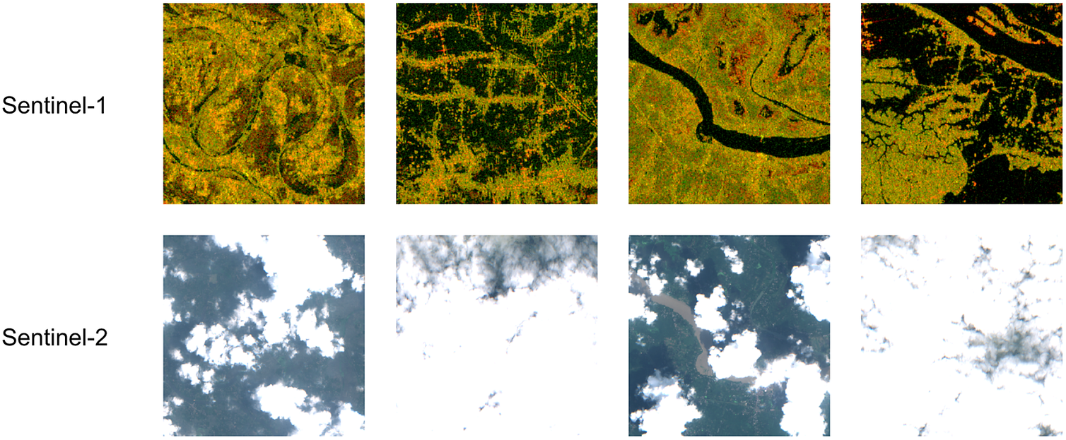
Figure 1. Selectively sampled Sentinel-1 and Sentinel-2 images taken during flooding events.
Note: Clouds are heavily correlated with flooding events, and these examples visualize some Sentinel-2 images during such events. On the other hand, SAR images can see through the clouds and serve as a more useful input for segmentation models during flooding events.
Thresholding algorithms (Martinis and Rieke, Reference Martinis and Rieke2015; Brown et al., Reference Brown, Hambidge and Brownett2016; Liang and Liu, Reference Liang and Liu2020) are traditionally used to segment flooded regions from SAR images since water has a low backscatter intensity. Commonly used techniques like Otsu thresholding (Bao et al., Reference Bao, Lv and Yao2021) assume that the histogram of a SAR image has a bimodal distribution, which works well for many cases. However, its failure modes include generating false positives for mountain shadows and generating excessive background noise due to speckle in SAR imagery. This noise can be removed using Lee speckle filters (Lee, Reference Lee1981) or mean filters; however, this results in small streams being missed out. In recent years, convolutional neural networks (CNNs) have been used to segment flooded areas from satellite images. Unlike traditional pixel-wise methods, they can look at a larger context and incorporate spatial features from an image. Mateo-Garcia et al. (Reference Mateo-Garcia, Veitch-Michaelis, Smith, Oprea, Schumann, Gal, Baydin and Backes2021) and Akiva et al. (Reference Akiva, Purri, Dana, Tellman and Anderson2021) have focused on using opportunistically available cloud-free Sentinel-2 images. Although these methods have good performance, their utility at inference time is limited because of the cloud cover issues mentioned previously. Another line of work fuses Sentinel-1 and Sentinel-2 images (Tavus et al., Reference Tavus, Kocaman, Nefeslioglu and Gokceoglu2020; Bai et al., Reference Bai, Wu, Yang, Yu, Zhao, Liu, Yang, Mas and Koshimura2021; Konapala et al., Reference Konapala, Kumar and Ahmad2021; Drakonakis et al., Reference Drakonakis, Tsagkatakis, Fotiadou and Tsakalides2022) to enhance surface water detection during flooded events. These methods not only require a cloud-free Sentinel-2 imaget also require that both images are acquired at about the same time to avoid alignment issues. There also has been some work done that uses multi-temporal images (Zhang et al., Reference Zhang, Chen, Liang, Tian and Yang2020; Sunkara et al., Reference Sunkara, Leach and Ganju2021; Yadav et al., Reference Yadav, Nascetti and Ban2022) containing a pre-flood and a post-flood event. These methods do change detection and exhibit better performance. In our work, however, we focus on methods that only take a single Sentinel-1 timestamp image as input.
Sen1Floods11 (Bonafilia et al., Reference Bonafilia, Tellman, Anderson and Issenberg2020) is a popular dataset for flood segmentation, which was used in prior work that takes a single Sentinel-1 image as input (Katiyar et al., Reference Katiyar, Tamkuan and Nagai2021; Ghosh et al., Reference Ghosh, Garg and Motagh2022; Helleis et al., Reference Helleis, Wieland, Krullikowski, Martinis and Plank2022). It is publicly available and has a small set of high-quality hand-labeled images and a larger set of weak-labeled images. However, the limitation of using weak-labeled data (despite using various regularization techniques) is that the model still learns the mistakes present in those labels. Previously, Wang et al. (Reference Wang, Liu and Tao2017), Song et al. (Reference Song, Kim and Lee2019), Huang et al. (Reference Huang, Zhang and Zhang2020), and Zheng et al. (Reference Zheng, Awadallah and Dumais2021) have explored to handle noisy label using loss adjustment. Wang et al. (Reference Wang, Liu and Tao2017) use loss re-weighting to assign a lower weight to incorrect labels, and Song et al. (Reference Song, Kim and Lee2019) and Huang et al. (Reference Huang, Zhang and Zhang2020) employ label refurbishing by using entropy to correct noisy labels or by doing a progressive refinement of the noisy labels using a combination of the current model output and the label. Zheng et al. (Reference Zheng, Awadallah and Dumais2021) proposes a meta-learning-based framework, where a label correction model is trained to correct the noisy labels and the main model is trained on these corrected labels. However, most of these methods have only been explored for classification and are hard to optimize for segmentation tasks due to increased complexity. Our work also explores methods to do label correction; however, we use a simpler idea of using historical temporal imagery to correct weak labels during training as described in Section 3.2.
In contrast to the above work, we also explore leveraging unlabeled data through semi-supervised learning techniques as opposed to creating weak labels. Methods such as those used by Sohn et al. (Reference Sohn, Berthelot, Carlini, Zhang, Zhang, Raffel, Cubuk, Kurakin and Li2020), Paul and Ganju (Reference Paul and Ganju2021), Ahmed et al. (Reference Ahmed, Morerio and Murino2022), and Wang et al. (Reference Wang, Wang, Shen, Fei, Li, Jin, Wu, Zhao and Le2022) have explored semi-supervised techniques to make use of both labeled and unlabeled data. The basic principle of the method used by Sohn et al. (Reference Sohn, Berthelot, Carlini, Zhang, Zhang, Raffel, Cubuk, Kurakin and Li2020) is that it uses pseudo labels predicted on the weak augmented image to consistently train heavily augmented images. Ahmed et al. (Reference Ahmed, Morerio and Murino2022) ensemble predictions from multiple augmentations to produce more noise resilient labels. However, most of these works focus on RGB images and their performance degrades in remote sensing images. This happens because most of the augmentations are handcrafted for RGB images only. Motivated to use different modalities of satellite data of the same location as natural augmentations in semi-supervised methods and cross-modal feature distillation (Gupta et al., Reference Gupta, Hoffman and Malik2016), we use a teacher–student setup that extracts information from a more informative modality (Sentinel-2) to supervise paired Sentinel-1 SAR images with the help of a small hand-labeled and a large unlabeled dataset. Similar to the work of Gupta et al. (Reference Gupta, Hoffman and Malik2016), we transfer supervision between different modalities. However, instead of supervising an intermediate feature layer as mentioned in the study Gupta et al. (Reference Gupta, Hoffman and Malik2016), we transfer supervision at the output layer and apply this toward a new application (i.e., flood segmentation). Our main contribution in this work are:
-
• We propose a cross-modal distillation framework and apply it to transfer supervision between different modalities using paired unlabeled data.
-
• We propose a method to improve the quality of weak labels using past temporal data and use that to enhance the weak-label baseline.
-
• We curate an additional large dataset (in addition to Sen1Floods11) from various flooding events containing paired Sentinel-1 and Sentinel-2 images and a weak label based on Sentinel-2 data.
The remainder of this paper is structured as follows. A description of the datasets is provided in Section 2, followed by a detailed explanation of our method in Section 3. The training details and a summary of the results are presented in Section 4, and a sensitivity analysis is discussed in Section 5. Finally, conclusions are stated in Section 6.
2. Data
2.1. Data features
2.1.1. Sentinel-1 image
Sentinel-1 (Torres et al., Reference Torres, Snoeij, Geudtner, Bibby, Davidson, Attema, Potin, Rommen, Floury, Brown, Traver, Deghaye, Duesmann, Rosich, Miranda, Bruno, L’Abbate, Croci, Pietropaolo, Huchler and Rostan2012) mission launched by European Space Agency (ESA) consists of two polar orbiting satellites to provide free SAR data. However, recently, one of the satellite malfunctioned and currently remains out of service. ESA has plans to launch another satellite in 2023. This satellite is an example of an active remote sensing satellite and uses radio waves operating at a center frequency of 5.405 GHz, which allows it to see through cloud cover. It has a spatial resolution of 10 m and has a return period of 6 days. We use the Sentinel-1 GRD product and utilize the bands that consist of dual polarized data: vertical transmit-vertical receive (VV) and vertical transmit-horizontal receive (VH). These bands representing the backscatter coefficient are converted to logarithmic (dB) scale. The backscatter coefficient is mainly influenced by the physical characteristics such as roughness and the geometry of the terrain and the dielectric constant of the surface. It is discriminative for detecting surface water, as water specularly reflects away all the emitted radiation from the satellite.
2.1.2. Sentinel-2 image
Sentinel-2 (Drusch et al., Reference Drusch, del Bello, Carlier, Colin, Fernandez, Gascon, Hoersch, Isola, Laberinti, Martimort, Meygret, Spoto, Sy, Marchese and Bargellini2012) mission was also launched by the ESA and has two polar orbiting satellites. It provides multispectral data at a resolution of 10 m and has a return period of 5 days. We use the L1-C Top of Atmosphere (TOA) product. It is a passive remote sensing satellite operating in visible and infrared wavelength. Its images are affected by atmospheric conditions and often contain significant cloud cover. The multispectral data consist of 13 bands, and in this work, we use four bands: B2 (blue), B3 (green), B4 (red), and B8 (NIR). These bands are used for various tasks like land cover/use monitoring, climate change, and disaster monitoring.
2.1.3. Weak label
The weak labels are computed from the Sentinel-2 image. Although cloud-free Sentinel-2 data are rarely available during a flooding event, we can still opportunistically sample timestamps from a long time range and get enough cloud-free views. Initially, the cloud mask is estimated using Sentinel-2 quality assurance band (QA60). The cloud mask is then dilated to mask out the nearby cloud shadows as the spectral signature of the cloud shadows is similar to that of water (Li et al., Reference Li, Sun and Yu2013). Weak flood labels are then created by thresholding the normalized difference water index (NDWI) ( $ NDWI=\left(B3-B8\right)/\left(B3+B8\right) $
) band. The pixels having value greater than 0 are marked as water and the rest are marked dry.
$ NDWI=\left(B3-B8\right)/\left(B3+B8\right) $
) band. The pixels having value greater than 0 are marked as water and the rest are marked dry.
2.1.4. Water occurrence map
The water occurrence map (Pekel et al., Reference Pekel, Cottam, Gorelick and Belward2016) shows how water is distributed temporally throughout the 1984–2020 period. It provides the probability of each pixel being classified as water averaged over the above time period at a spatial resolution of 30 m. The data were generated using optical data from Landsat 5, 7, and 8. This map can be used to capture both the intra- and inter-annual changes and to differentiate seasonal/ephemeral flooding pixels from permanent water pixels. Each pixel was individually classified into water/non-water using an expert system, and the results were collated into a monthly history for the entire time period. Averaging the results of all monthly calculations gives the long-term overall surface water occurrence.
2.2. Datasets
2.2.1. Sen1Floods11 dataset
This is a publicly available dataset (Bonafilia et al., Reference Bonafilia, Tellman, Anderson and Issenberg2020) containing 4,831 tiles from 11 flooding events across six continents. It contains paired Sentinel-1 SAR and Sentinel-2 multi-spectral images. Each tile is $ 512\times 512 $
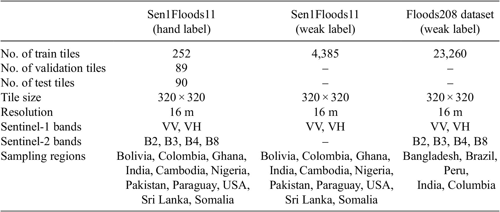
pixels at a resolution of 10 m per pixel. Due to the high cost of labeling, only 446 tiles out of 4,831 are hand labeled by remote sensing experts to provide high-quality flood water labels. The authors provide an IID split of these hand-labeled tiles, containing 252 training, 89 validation, and 90 test sample chips. The remaining 4,385 tiles have weak labels prepared by thresholding normalized difference vegetation index (NDVI) and modified normalized difference water index (MNDWI) values. The weak labels are only used for training. We also augment the dataset with the water occurrence map for every tile.
$ 512\times 512 $
pixels at a resolution of 10 m per pixel. Due to the high cost of labeling, only 446 tiles out of 4,831 are hand labeled by remote sensing experts to provide high-quality flood water labels. The authors provide an IID split of these hand-labeled tiles, containing 252 training, 89 validation, and 90 test sample chips. The remaining 4,385 tiles have weak labels prepared by thresholding normalized difference vegetation index (NDVI) and modified normalized difference water index (MNDWI) values. The weak labels are only used for training. We also augment the dataset with the water occurrence map for every tile.
2.2.2. Floods208 dataset
We curated additional imagery by downloading closely acquired Sentinel-1 and Sentinel-2 images from Earth Engine (Gorelick et al., Reference Gorelick, Hancher, Dixon, Ilyushchenko, Thau and Moore2017) during flood events provided to us by external partners.
The data are extracted using the following steps:
-
• For each data point consisting of latitude, longitude, and flooding event timestamp, get the Sentinel-1 image of the area of interest (AOI).
-
• Search for overlapping Sentinel-2 images within 12 h of Sentinel-1 timestamp. Filter out images with $ >12\% $
cloud cover.
$ >12\% $
cloud cover. -
• Pick the Sentinel-2 image closest to Sentinel-1 timestamp from the filtered images. If none are available, we discard this data point.

The data points were extracted from 208 flooding events across Bangladesh, Brazil, Colombia, India, and Peru. These regions are shown in Figure 2 and were chosen according to the regions of interest for final deployment. We also extracted the water occurrence map and a weak label for each image using the NDWI band from the Sentinel-2 image. The extracted images had a resolution of 16 m per pixel. Each image from a flooding event was then partitioned into multiple small tiles of size $ 320\times 320 $
. The tiles at the edge of image were padded to fit the
$ 320\times 320 $
. The tiles at the edge of image were padded to fit the $ 320\times 320 $
tile size. Tiles having cloud percentage greater than
$ 320\times 320 $
tile size. Tiles having cloud percentage greater than $ 80\% $
were discarded. In total, 23,260 valid tiles of size
$ 80\% $
were discarded. In total, 23,260 valid tiles of size $ 320\times 320 $
were extracted from the whole process. Figure 3 shows some selected data points from both the datasets.
$ 320\times 320 $
were extracted from the whole process. Figure 3 shows some selected data points from both the datasets.
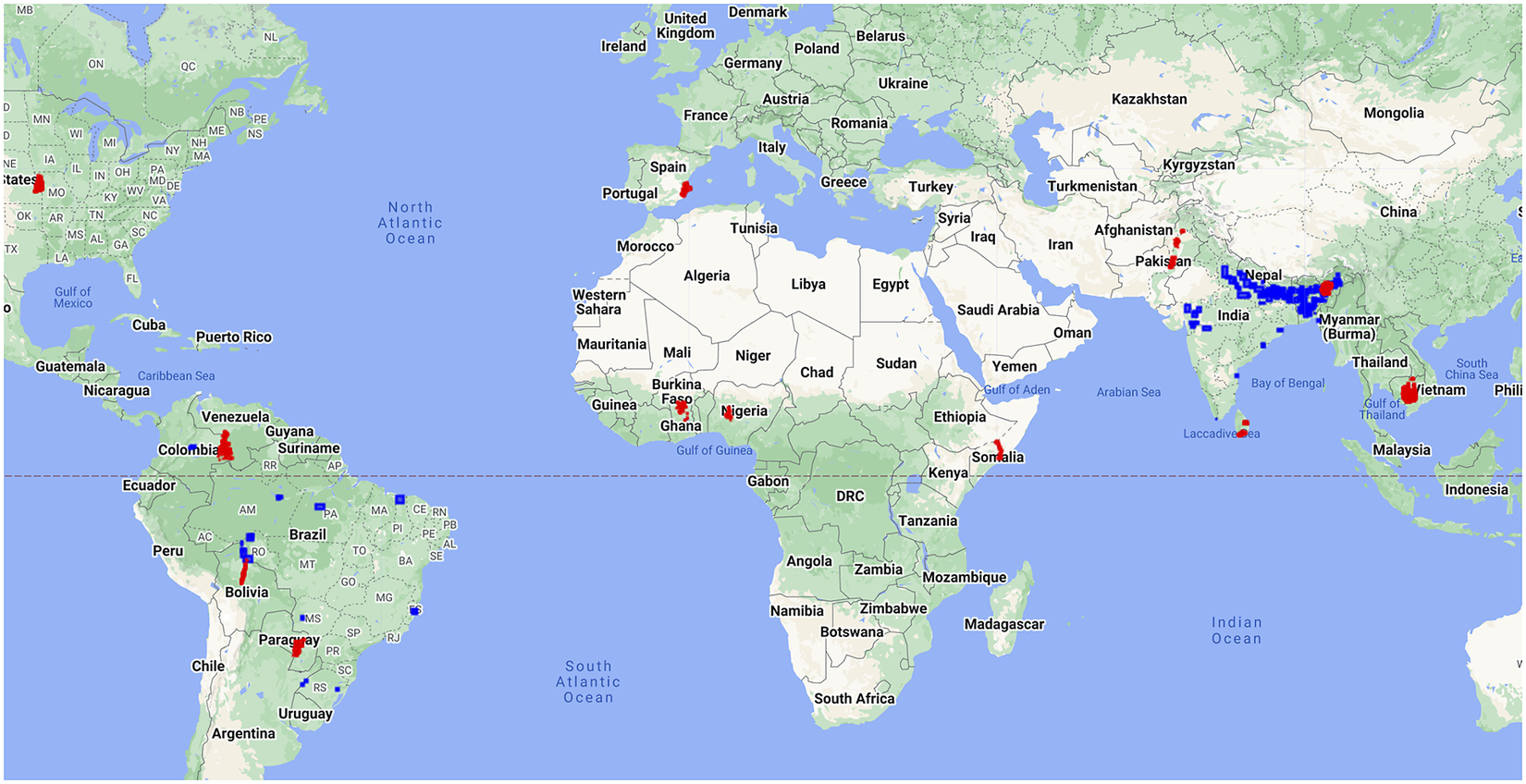
Figure 2. Red points highlight the regions from where Sen1Floods11 flooding event data points were sampled, and blue points indicate the same for Floods208 dataset.
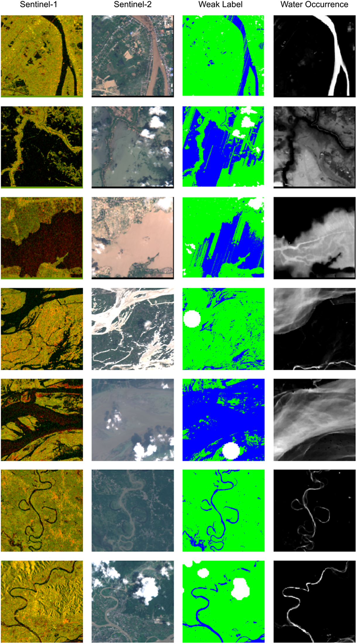
Figure 3. Selectively sampled data points from Sen1Floods11 weak-labeled data (first three rows) and Floods208 Dataset (last four rows).
Note: In the weak label, the mapping is green: dry, blue: water, and white: clouded/invalid pixels. These examples highlight the poor quality of the weak labels.
2.3. Preprocessing
The provided Sen1Floods11 dataset has latitude/longitude projection (based on the WGS84 datum, i.e., EPSG:4326) and has a resolution of 10 m per pixel. To match the projection and resolution of our Floods208 dataset, all the images are scaled to 16 m per pixel input resolution and projected to the Universal Transverse Mercator (UTM) coordinate system. For Sentinel-1 image normalization, VV band was clipped to [−20, 0] and VH to [−30, 0] and then linearly scaled these values to the range [0, 1]. For Sentinel-2 image, the four bands were clipped to [0, 3,000] range and then linearly scaled them to [0, 1] range. Table 1 summarizes the final attributes of both the datasets.
Table 1. Summary of the key attributes of all the datasets used for training and evaluation
3. Methods
Our aim is to segment flooded pixels using Sentinel-1 SAR image as an input at inference time. Formally, let $ {X}_{S1}\in {R}^{H\times W\times 2} $
be the SAR input space and let
$ {X}_{S1}\in {R}^{H\times W\times 2} $
be the SAR input space and let $ Y\in {R}^{H\times W\times K} $
denote the pixel-wise
$ Y\in {R}^{H\times W\times K} $
denote the pixel-wise $ K $
class one hot label in the output space (
$ K $
class one hot label in the output space ( $ K=2 $
classes in our case: dry and flooded pixels). The paired Sentinel-2 images used in the training data are represented by
$ K=2 $
classes in our case: dry and flooded pixels). The paired Sentinel-2 images used in the training data are represented by $ {X}_{S2}\in {R}^{H\times W\times 4} $
. The hand-labeled training set is denoted by
$ {X}_{S2}\in {R}^{H\times W\times 4} $
. The hand-labeled training set is denoted by $ {D}_l={\left\{{X}_{S1}^i,{X}_{S2}^i,{Y}^i\right\}}_{i=1}^{N_l} $
and the larger weak-labeled training set as
$ {D}_l={\left\{{X}_{S1}^i,{X}_{S2}^i,{Y}^i\right\}}_{i=1}^{N_l} $
and the larger weak-labeled training set as $ {D}_{wl}={\left\{{X}_{S1}^i,{X}_{S2}^i,{\hat{Y}}^i\right\}}_{i=1}^{N_{wl}} $
. Here,
$ {D}_{wl}={\left\{{X}_{S1}^i,{X}_{S2}^i,{\hat{Y}}^i\right\}}_{i=1}^{N_{wl}} $
. Here, $ Y $
denotes a high-quality label and
$ Y $
denotes a high-quality label and $ \hat{Y} $
denotes a noisy weak label. Our goal is to leverage both
$ \hat{Y} $
denotes a noisy weak label. Our goal is to leverage both $ {D}_l $
and
$ {D}_l $
and ![]() to train the segmentation network. The next section describes the supervised baseline, an approach to improve weak labels and the cross-modal distillation framework.
to train the segmentation network. The next section describes the supervised baseline, an approach to improve weak labels and the cross-modal distillation framework.
3.1. Supervised baseline
We train two supervised models for comparison. The first model is trained only on hand-labeled data $ {D}_l $
. The second model is trained only on the larger weak-labeled dataset
$ {D}_l $
. The second model is trained only on the larger weak-labeled dataset $ {D}_{wl} $
. The large size of the weak-labeled data helps the network to generalize better (despite the model learning some of those label errors during training; Rolnick et al., Reference Rolnick, Veit, Belongie and Shavit2017). We use Deeplab v3+ (Chen et al., Reference Chen, Zhu, Papandreou, Schroff and Adam2018) with an Xception 65 encoder (Chollet, Reference Chollet2017) as the model architecture. Common regularization techniques like data augmentations (random crop with distortion, horizontal/vertical flips, and color jitter), dropout, weight decay, and batch normalization are used to improve generalization. We also tried to fine-tune the second model, that is, the model trained on weak-labeled data, using hand-labeled data
$ {D}_{wl} $
. The large size of the weak-labeled data helps the network to generalize better (despite the model learning some of those label errors during training; Rolnick et al., Reference Rolnick, Veit, Belongie and Shavit2017). We use Deeplab v3+ (Chen et al., Reference Chen, Zhu, Papandreou, Schroff and Adam2018) with an Xception 65 encoder (Chollet, Reference Chollet2017) as the model architecture. Common regularization techniques like data augmentations (random crop with distortion, horizontal/vertical flips, and color jitter), dropout, weight decay, and batch normalization are used to improve generalization. We also tried to fine-tune the second model, that is, the model trained on weak-labeled data, using hand-labeled data $ {D}_l $
. However, this additional training step did not improve the performance, so we decided not to include it in the baseline model.
$ {D}_l $
. However, this additional training step did not improve the performance, so we decided not to include it in the baseline model.
3.1.1. Edge-weighted loss
The network is trained to minimize the cross-entropy loss. For every batch of images ( $ {B}_{wl} $
), the parameters
$ {B}_{wl} $
), the parameters $ f $
of the network are updated by minimizing the cross-entropy loss given by:
$ f $
of the network are updated by minimizing the cross-entropy loss given by:
 $$ L=\frac{1}{B_{wl}}\sum {l}_{ce}\left(f\left({X}_i\right),{\hat{Y}}_i,{W}_i\right). $$
Here, $ {W}_i $
represents the pixel-wise weights for the
$ {W}_i $
represents the pixel-wise weights for the $ i $
th image—
$ i $
th image— $ {X}_i $
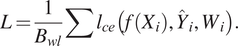
, applied to the cross-entropy loss. We apply an edge-based weighting that gives higher weights to the edges of the binary label. As suggested by Wu et al. (Reference Wu, Shen and van den Hengel2016), from all the pixels in an image available for training, the pixels lying in the middle of an object can be easily discriminated by the model and are usually classified correctly. Hence, an edge-weighted loss helps the network to focus on the harder-to-segment regions lying on the boundary during training. We compute two kinds of edges, inner and outer edges. Inner edges are obtained by subtracting the eroded labels from the original labels. Outer edges are obtained by subtracting the original labels from the dilated labels. All the other pixels are given a unit weight. The weights for inner and outer edges are decided by tuning these parameters during training. Figure 4 shows these edges.
$ {X}_i $
, applied to the cross-entropy loss. We apply an edge-based weighting that gives higher weights to the edges of the binary label. As suggested by Wu et al. (Reference Wu, Shen and van den Hengel2016), from all the pixels in an image available for training, the pixels lying in the middle of an object can be easily discriminated by the model and are usually classified correctly. Hence, an edge-weighted loss helps the network to focus on the harder-to-segment regions lying on the boundary during training. We compute two kinds of edges, inner and outer edges. Inner edges are obtained by subtracting the eroded labels from the original labels. Outer edges are obtained by subtracting the original labels from the dilated labels. All the other pixels are given a unit weight. The weights for inner and outer edges are decided by tuning these parameters during training. Figure 4 shows these edges.
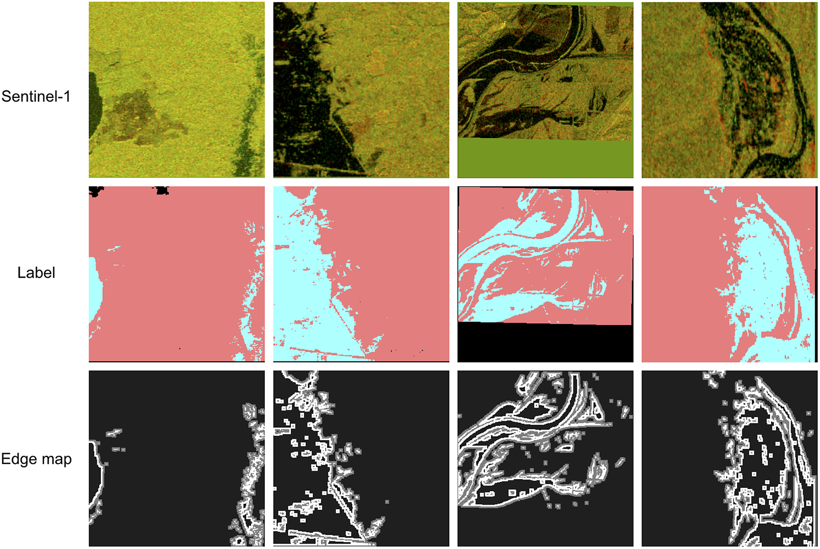
Figure 4. Randomly selected Sentinel-1 images from the training split with their corresponding label and edge map.
Note: In the label, blue pixels denote water, peach pixels denote dry region, and black pixels denotes the invalid pixels. The edge map shows the inner and outer edges in white and gray color, respectively.
3.2. Improving weak labels
Despite using regularization techniques, we notice that the model learns the label mistakes present in the training data. Figure 5 demonstrates this on the training set images. Often such mistakes consist of cases where a complete or a major part of the river is missing. While the network is resilient to learning small label mistakes (such as slightly overflooded pixels surrounding the true boundary or random noise similar to cut out augmentation), it does tend to overfit to cases when the label mistakes are large. This is because from an optimization perspective, pixels in an extremely noisy label dominate the loss, forcing the network to overfit on them in order to reduce the loss.
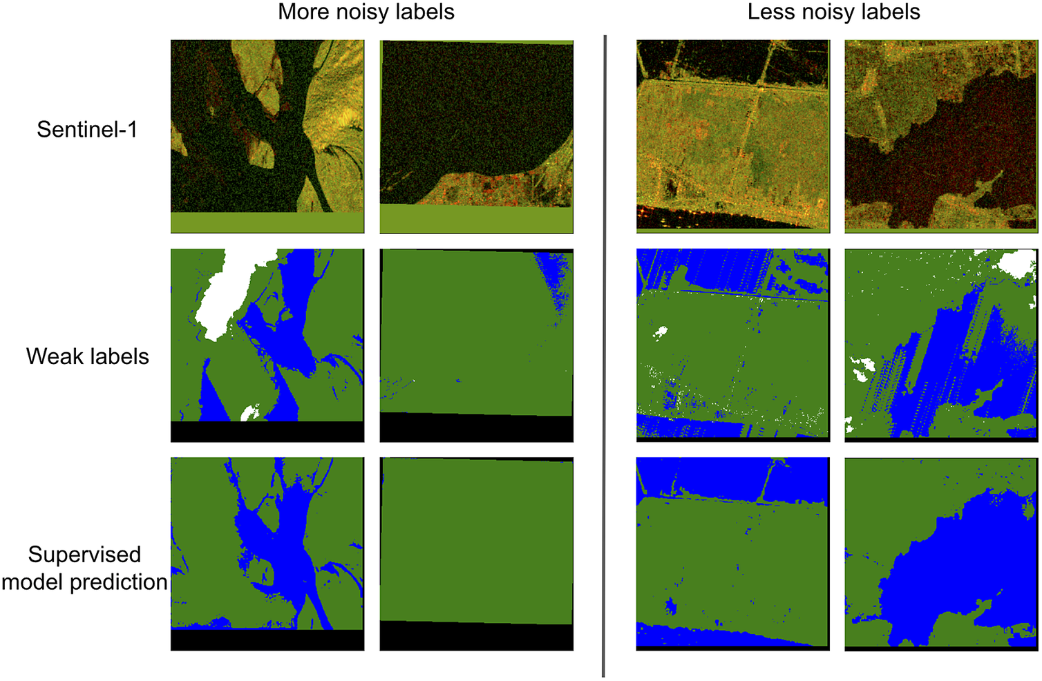
Figure 5. Selected examples from the training split demonstrating the effect of amount of label noise in memorizing the label mistakes.
Note: (Left) The model learns these mistakes when the label is of very poor quality and is missing most part of the river. (Right) The model can overcome these mistakes when there is less noise. The color scheme for the labels and prediction is the same as Figure 3, with the addition of black regions representing out-of-bounds pixels.
We aim to correct the labels having large parts of the river missing by using the water occurrence map to get a rough estimate of such missing rivers. The label initially misses the river because they are formed by thresholding Sentinel-2 image and the label is sensitive to the value of the threshold. Since the water occurrence map (Pekel et al., Reference Pekel, Cottam, Gorelick and Belward2016) is made by averaging long-term overall surface water occurrence, the permanent water pixels will have higher probability values and areas where water sometimes occurs will have lower probability values. The weak label is improved by additionally marking the pixels having their water occurrence probability above a certain threshold, as wet in the label. This method will not be able to capture the seasonal/flooded or ephemeral water pixels, but these pixels mostly constitute a small majority of the label, and as seen earlier, the model can learn to overcome such small mistakes in the labels. Figure 6 shows some randomly selected tiles before and after the label improvement from the training set.
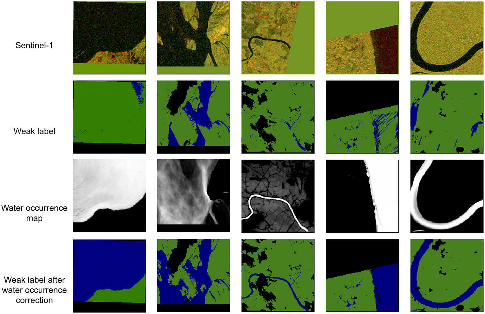
Figure 6. Improving weak label from the training split using the water occurrence map.
Note: The color scheme used in the weak label is the same as Figure 5.
3.3. Cross-modal distillation
Although the water occurrence map improved the weak labels in areas which are permanently water, it does not help with label mistakes in seasonal/flooded pixels. As a result, we can still get grossly incorrect weak labels in rare situations where flooded pixels constitute a majority portion of the water. To overcome this, we explore a cross-modal distillation framework that uses a network trained on a richer modality with a small set of hand labels to generate more accurate labels on the training split. A teacher–student setup is used to transfer supervision between the two modalities. The teacher is trained on stacked Sentinel-1 and Sentinel-2 images using accurate labels from $ {D}_l $
, and is used to supervise a Sentinel-1-only student model on the unlabeled images from
$ {D}_l $
, and is used to supervise a Sentinel-1-only student model on the unlabeled images from $ {D}_{wl} $
. The advantage of this method over binary weak labels (used in Section 3.1) is that the soft labels predicted by the teacher capture uncertainty better compared to the binary labels (Ba and Caruana, Reference Ba and Caruana2014; Hinton et al., Reference Hinton, Vinyals and Dean2015). The soft targets are also outputs of a network trained on hand-labeled data and are more likely to be correct than weak labels. Compared to self-distillation, cross-modal distillation enables us to provide more accurate supervision by transferring information from a richer knowledge modality. Figure 7 summarizes the training setup used in our work. Both the teacher and the student have identical architecture backbones. Let
$ {D}_{wl} $
. The advantage of this method over binary weak labels (used in Section 3.1) is that the soft labels predicted by the teacher capture uncertainty better compared to the binary labels (Ba and Caruana, Reference Ba and Caruana2014; Hinton et al., Reference Hinton, Vinyals and Dean2015). The soft targets are also outputs of a network trained on hand-labeled data and are more likely to be correct than weak labels. Compared to self-distillation, cross-modal distillation enables us to provide more accurate supervision by transferring information from a richer knowledge modality. Figure 7 summarizes the training setup used in our work. Both the teacher and the student have identical architecture backbones. Let $ {f}_t $
and
$ {f}_t $
and $ {f}_s $
represent the teacher and student network function, respectively. The training is done in two stages as described below:
$ {f}_s $
represent the teacher and student network function, respectively. The training is done in two stages as described below:
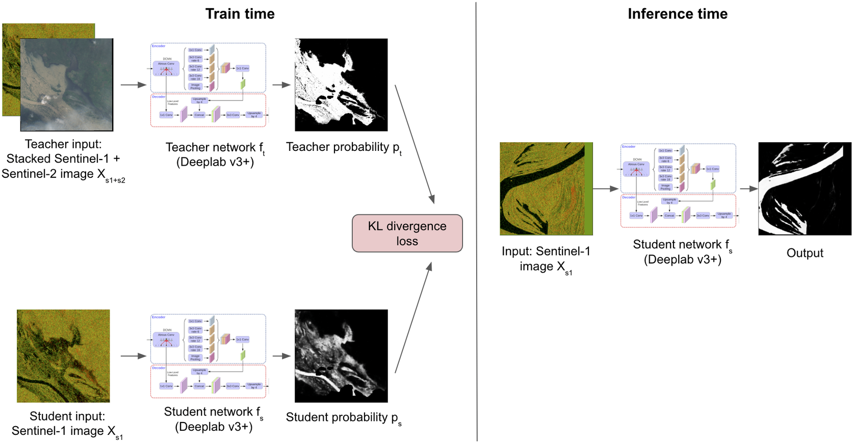
Figure 7. Overview of our cross-modal distillation framework.
Note: In the training stage, a teacher model using Sentinel-1 and Sentinel-2 images is used to train a student using only the Sentinel-1 image. At inference time, only the student is used to make predictions.
Stage 1: Training the teacher network. Let $ {X}_{S1+S2}^i $
denote the
$ {X}_{S1+S2}^i $
denote the $ i $
th stacked Sentinel-1 and Sentinel-2 image.
$ i $
th stacked Sentinel-1 and Sentinel-2 image. $ {X}_{S1+S2}^i\in {D}_l $
is used as input to the teacher network. The teacher is trained in the same manner as the supervised baseline described in Section 3.1. The training set is small but contains data from geographic locations spanning six different continents. This helps the teacher generalize well to different geographies in the unlabeled data seen during the next stage of training.
$ {X}_{S1+S2}^i\in {D}_l $
is used as input to the teacher network. The teacher is trained in the same manner as the supervised baseline described in Section 3.1. The training set is small but contains data from geographic locations spanning six different continents. This helps the teacher generalize well to different geographies in the unlabeled data seen during the next stage of training.
Stage 2: Training the student network. The teacher weights from Stage 1 are kept frozen in this stage. We use paired Sentinel-1 and Sentinel-2 images from Sen1Floods11 data (i.e., both hand labeled and weak labeled) and Floods208 weak-labeled data as the unlabeled data to train the student network. The data in each batch are sampled equally from both the data sources to ensure equal weighting for the datasets. The stacked Sentinel-1 and Sentinel-2 image $ {X}_{S1+S2}^i $
is passed through the teacher to obtain the probabilities
$ {X}_{S1+S2}^i $
is passed through the teacher to obtain the probabilities $ {p}_t=\sigma \left({f}_t\left({X}_{S1+S2}^i\right)\right) $
and the augmented paired Sentinel-1 image
$ {p}_t=\sigma \left({f}_t\left({X}_{S1+S2}^i\right)\right) $
and the augmented paired Sentinel-1 image $ {\tilde{X}}_{S1}^i= Aug\left({X}_{S1}^i\right) $
is passed through the student to get the student probabilities
$ {\tilde{X}}_{S1}^i= Aug\left({X}_{S1}^i\right) $
is passed through the student to get the student probabilities $ {p}_s=\sigma \left({f}_s\left({\tilde{X}}_{S1}^i\right)\right) $
. Here,
$ {p}_s=\sigma \left({f}_s\left({\tilde{X}}_{S1}^i\right)\right) $
. Here, $ \sigma $
refers to the softmax function used to convert the model’s output into a probability score. KL divergence loss (
$ \sigma $
refers to the softmax function used to convert the model’s output into a probability score. KL divergence loss ( $ {L}_{KD} $
) is then minimized for
$ {L}_{KD} $
) is then minimized for $ K=2 $
classes to update the student weights:
$ K=2 $
classes to update the student weights:
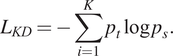 $$ {L}_{KD}=-\sum \limits_{i=1}^K{p}_t\log {p}_s. $$
4. Experiments and results
4.1. Training details
For all the models, we use DeepLab v3+ model (Chen et al., Reference Chen, Zhu, Papandreou, Schroff and Adam2018) with Xception 65 (Chollet, Reference Chollet2017) as the backbone encoder. DeepLab v3+ is a widely used semantic segmentation architecture that has previously shown state-of-the-art results on several benchmark datasets like PASCAL VOC (Everingham et al., Reference Everingham, Van Gool, Williams, Winn and Zisserman2010) and Cityscapes (Cordts et al., Reference Cordts, Omran, Ramos, Rehfeld, Enzweiler, Benenson, Franke, Roth and Schiele2016). It uses atrous convolution (Chen et al., Reference Chen, Zhu, Papandreou, Schroff and Adam2018) in its backbone encoder to learn features at different scales without degrading the spatial resolution and affecting the number of parameters. DeepLab v3+ adapted Xception 65 as its main feature extractor (encoder). Xception 65 is a 65-layer convolution neural network architecture that uses depth-wise separable convolution layers. DeepLab v3+ also employs an effective decoder module consisting of skip connections from the corresponding low-level encoder features at different scales to output enhanced segmentation results. In our experiments, we use a skip connection from the encoder features at scales $ 1/4 $
and
$ 1/4 $
and $ 1/2 $
.
$ 1/2 $
.
We use a batch size of 64 with input image shape of $ \left(\mathrm{321,321},C\right) $
(here,
$ \left(\mathrm{321,321},C\right) $
(here, $ C=2 $
for Sentinel-1 images and
$ C=2 $
for Sentinel-1 images and $ C=4 $
for Sentinel-2 images). For input images having height and width dimensions less than
$ C=4 $
for Sentinel-2 images). For input images having height and width dimensions less than $ 321 $
, zero padding is done. During training, crop distortion augmentation with distortion parameter
$ 321 $
, zero padding is done. During training, crop distortion augmentation with distortion parameter $ d=0.5 $
is applied on the input images. Here, a random crop is taken between
$ d=0.5 $
is applied on the input images. Here, a random crop is taken between $ \left[\left(1-d\right)\ast 321,\left(1+d\right)\ast 321\right] $
unit length and then stretched to the desired crop size that is
$ \left[\left(1-d\right)\ast 321,\left(1+d\right)\ast 321\right] $
unit length and then stretched to the desired crop size that is $ \left(\mathrm{321,321}\right) $
. As a result,
$ \left(\mathrm{321,321}\right) $
. As a result, $ 1 $
unit length on original image will get stretched randomly between
$ 1 $
unit length on original image will get stretched randomly between $ \left[1-d,1+d\right] $
unit length. We also apply random horizontal and vertical flipping with probability
$ \left[1-d,1+d\right] $
unit length. We also apply random horizontal and vertical flipping with probability $ 0.5 $
, random
$ 0.5 $
, random $ 90\ast {k}^{\circ } $
rotation where
$ 90\ast {k}^{\circ } $
rotation where $ k $
is chosen uniformly from
$ k $
is chosen uniformly from $ \left\{\mathrm{0,1,2,3}\right\} $
with probability
$ \left\{\mathrm{0,1,2,3}\right\} $
with probability $ 1.0 $
, and color jitter augmentation similar to the study by Chen et al. (Reference Chen, Kornblith, Norouzi and Hinton2020) with probability
$ 1.0 $
, and color jitter augmentation similar to the study by Chen et al. (Reference Chen, Kornblith, Norouzi and Hinton2020) with probability $ 0.5 $
and strength parameter
$ 0.5 $
and strength parameter $ 5 $
.
$ 5 $
.
For optimization, momentum optimizer is used with momentum set to 0.9. The learning rate is decayed with a polynomial schedule from initial value to zero with a power of 0.9. The models are trained for 30 k steps. A learning rate, weight decay, and dropout grid search hyper-parameter tuning are done by choosing a learning rate from {0.3, 0.1, 0.003, 0.001}, weight decay from {1e-3, 1e-4, 1e-5, 1e-6}, and keeping probability from {0.7, 0.8, 0.9, 1.0}. Additionally, the inner and the outer edge weights for edge-weighted cross-entropy loss are also hyper-parameters that were tuned using contextual Gaussian process bandit optimization (Krause and Ong, Reference Krause and Ong2011). The search space for both inner and outer edge weights was $ \left[1,15\right] $
. A value of 10 for the inner edge and a value of 5 for the outer edge gave the best results on the validation set. A threshold of value 0.5 is used to create a binary mask of permanent water pixels from the water occurrence map. All the hyper-parameter tuning and best model checkpoint selection is done on the validation split. After the best checkpoint selection, the model is frozen and all the results are reported on the test split.
$ \left[1,15\right] $
. A value of 10 for the inner edge and a value of 5 for the outer edge gave the best results on the validation set. A threshold of value 0.5 is used to create a binary mask of permanent water pixels from the water occurrence map. All the hyper-parameter tuning and best model checkpoint selection is done on the validation split. After the best checkpoint selection, the model is frozen and all the results are reported on the test split.
4.2. Evaluation metric
We use pixel-wise intersection over union (IoU) of the water class to validate our model performance. It is defined as follows:
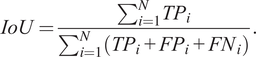 $$ IoU=\frac{\sum_{i=1}^N{TP}_i}{\sum_{i=1}^N\left({TP}_i+{FP}_i+{FN}_i\right)}. $$
In the above formula, $ i $
iterates over all the images and
$ i $
iterates over all the images and $ N $
is the total number of images. For the
$ N $
is the total number of images. For the $ i $
th image,
$ i $
th image, $ {TP}_i $
,
$ {TP}_i $
, $ {FP}_i $
, and
$ {FP}_i $
, and $ {FN}_i $
denote the number of true positives, false positives, and false negatives of water class, respectively.
$ {FN}_i $
denote the number of true positives, false positives, and false negatives of water class, respectively.
4.3. Results
4.3.1. Comparison with our baselines
Table 2 presents the result of the supervised baseline model trained on the Sen1Floods11 hand-labeled data. As expected, the model using Sentinel-2 as its input performs much better than the models using Sentinel-1 because Sentinel-2 is a richer modality. However, the Sentinel-2 image is not suitable for inference because of cloud cover issues mentioned in Section 2.1. Due to this reason, while we cannot use the model using stacked Sentinel-1 and Sentinel-2 image during inference, we can opportunistically utilize this as a richer set of features to train the teacher model for cross-modal distillation as discussed in Section 3.3.
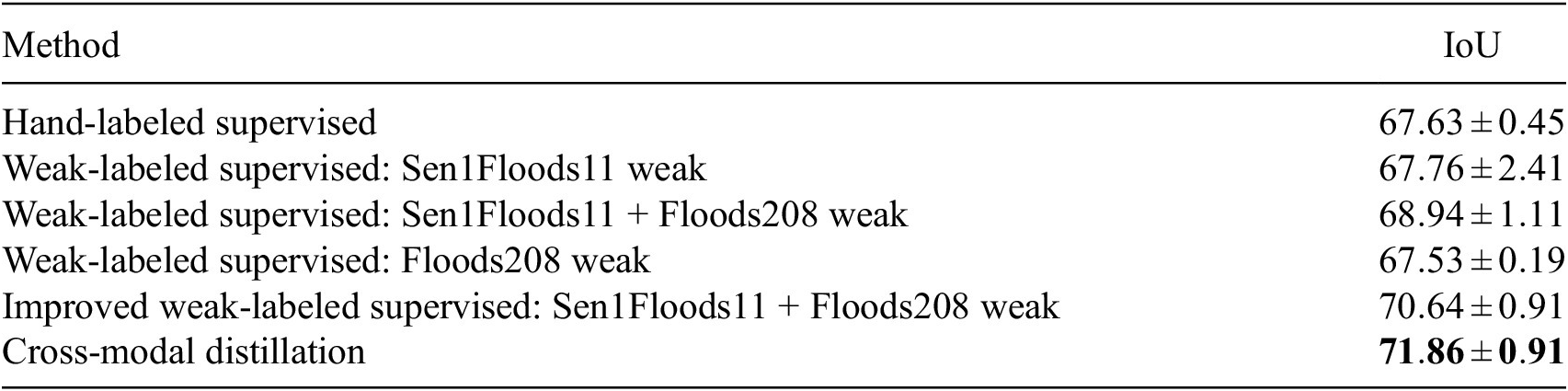
Table 2. Test split results of our model trained on Sen1Floods11 hand-labeled data at 16 m resolution
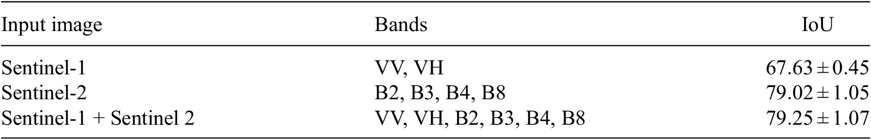
Note. The numbers show the aggregated mean and standard deviation of IoU from five runs.
Table 3 presents a quantitative comparison of the supervised baseline method with the model trained after improving the weak labels and the cross-distillation model. In the first two rows of Table 3, it can be seen that a supervised model trained on Sentinel-2 weak label can match the performance of a supervised model trained on small set of hand-labeled data. This empirically verifies the claim that a large weak-labeled dataset can act as a quick substitute for a small amount of costly hand-labeled annotations. Including Floods208 weak-labeled data to Sen1Floods11 weak-labeled data further led to an increase in the model performance by $ 1.18\% $
from Sen1Floods11 weak-label supervised baseline. This shows that there were still more gains to be had by increasing the weak-label dataset size. Even though Floods208 weak-labeled dataset by itself is also a very large dataset, the model trained on only Floods208 does not perform as well as the Sen1Floods11 weak-labeled data. This is because Floods208 data are localized to a smaller set of locations compared to the Sen1Floods11 weak-labeled split, which has data from six continents across the world. This emphasizes the importance of sampling training data strategically, such that the locations are more global and include various topographies. We can also see that improving weak labels using a water occurrence map as described in Section 3.2 increases the model IoU by
$ 1.18\% $
from Sen1Floods11 weak-label supervised baseline. This shows that there were still more gains to be had by increasing the weak-label dataset size. Even though Floods208 weak-labeled dataset by itself is also a very large dataset, the model trained on only Floods208 does not perform as well as the Sen1Floods11 weak-labeled data. This is because Floods208 data are localized to a smaller set of locations compared to the Sen1Floods11 weak-labeled split, which has data from six continents across the world. This emphasizes the importance of sampling training data strategically, such that the locations are more global and include various topographies. We can also see that improving weak labels using a water occurrence map as described in Section 3.2 increases the model IoU by $ 1.7\% $
compared with its weak supervised counterpart and by
$ 1.7\% $
compared with its weak supervised counterpart and by $ 2.88\% $
compared with the Sen1Floods11 weak-label baseline. This emphasizes the importance of quality of training labels in producing more accurate models. Our cross distillation model further improves the quality of training label using a teacher model and performs better than all the other models. It exceeds the Sen1Floods11 weak-label baseline by
$ 2.88\% $
compared with the Sen1Floods11 weak-label baseline. This emphasizes the importance of quality of training labels in producing more accurate models. Our cross distillation model further improves the quality of training label using a teacher model and performs better than all the other models. It exceeds the Sen1Floods11 weak-label baseline by $ 4.1\% $
IoU and improved weak-label supervised model by
$ 4.1\% $
IoU and improved weak-label supervised model by $ 1.22\% $
IoU. Figure 8 shows a qualitative comparison of the cross distillation model with the baseline model.
$ 1.22\% $
IoU. Figure 8 shows a qualitative comparison of the cross distillation model with the baseline model.
Table 3. Results of our Sentinel-1 supervised baseline models, improved weak-label supervised model, and our cross-modal distillation framework on Sen1Floods11 hand-label test split at 16 m resolution
Note. The numbers show the aggregated mean and standard deviation of IoU from five runs. The value in bold represents the top IoU metric value compared across all the models.
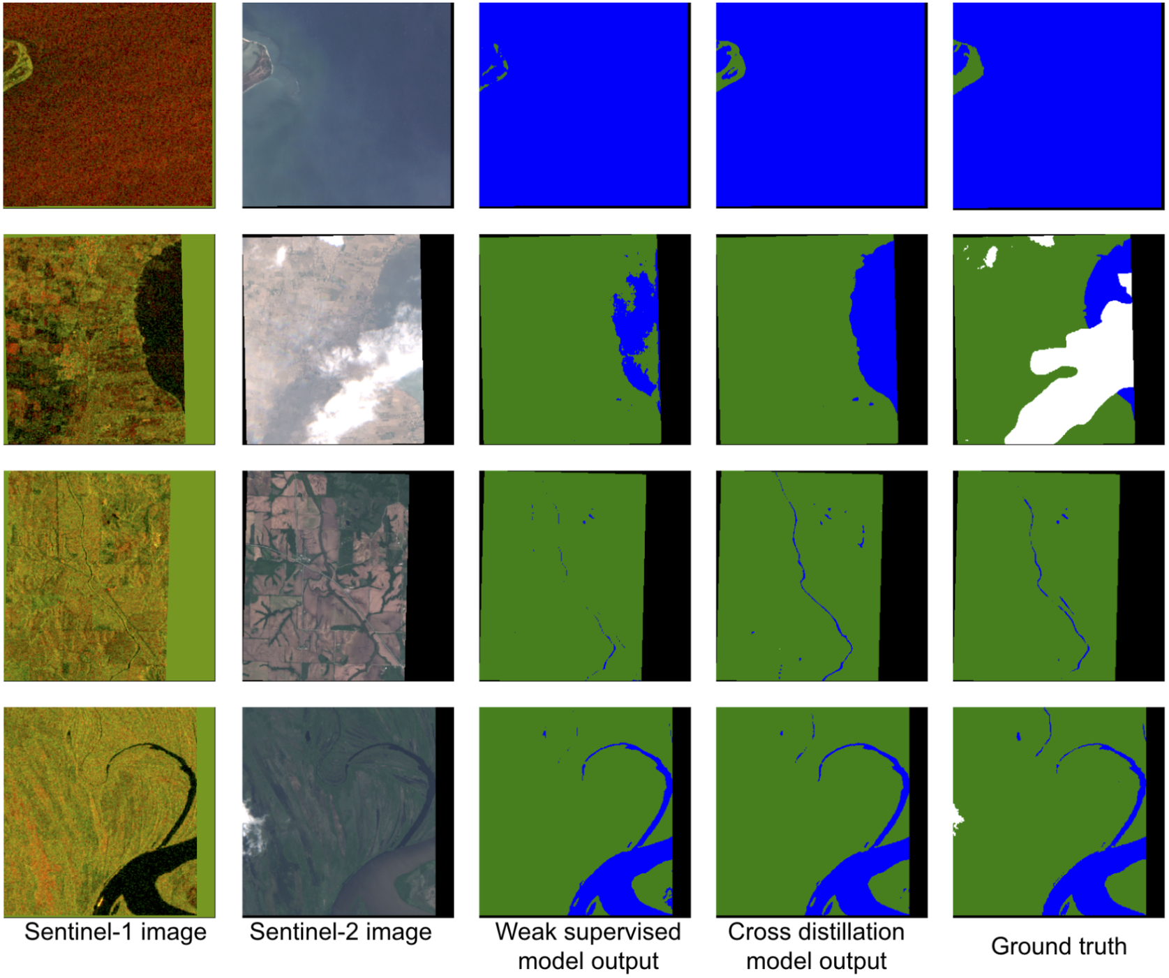
Figure 8. Model inference visualization on Sen1Floods11 hand-labeled test split on selected images.
Note: Here, the weak supervised model refers to the weak supervised baseline trained on Sen1Floods11 and Floods208 dataset. The color scheme used for the predictions and ground truth is the same as Figure 5. The Sentinel-2 image is not passed as input to the model and only shown for visualization purpose. The ground truth is hand labeled on the Sentinel-2 image and can contain clouds labeled in white color. It can be seen that cross-modal distillation produces sharper and more accurate results. Weak-labeled supervised baseline on the other hand sometimes misses big parts of river due to mistakes learnt from the training data.
Figure 9 analyzes the failure cases of the model. It can be seen that model sometimes struggles with segmenting water due to ambiguities in the Sentinel-1 image. We can also see that it sometimes fail to predict extremely thin rivers.
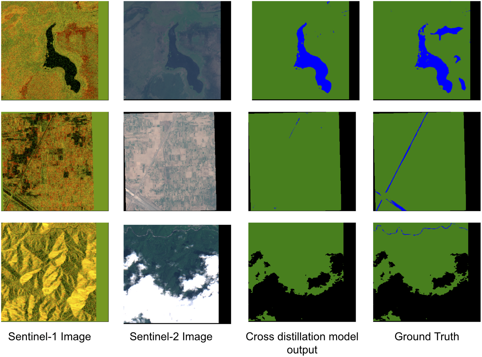
Figure 9. Selected examples showcasing the model’s failure case on Sen1Floods11 hand-labeled test split using the same color scheme as Figure 5.
Note: The Sentinel-2 image is not passed as input to the model and only shown for visualization purpose. The ground truth is hand labeled on the Sentinel-2 image. We can infer that the model struggles with segmenting water due to ambiguities in Sentinel-1 image. We can also see that it sometimes fails to detects extremely thin rivers
4.3.2. Comparison with other methods
Benchmark comparisons of IoU on Sen1Floods11 test split are provided in Table 4. Note that even though our method is trained at input images with resolution of 16 m, here, we do an evaluation at 10 m Sentinel-1 images and hand labels for a fair comparison with other methods. To get an inference output at a resolution of 10 m, we first downsample the original image of shape $ 512\times 512 $
to a resolution of 16 m that is
$ 512\times 512 $
to a resolution of 16 m that is $ 320\times 320 $
, feed the downsampled image to the model, and then upsample the probabilities to their original resolution.
$ 320\times 320 $
, feed the downsampled image to the model, and then upsample the probabilities to their original resolution.
Table 4. Performance comparison of our cross-modal distillation model with other methods on all water hand labels from Sen1Floods11 test set at 10 m resolution. The value in bold represents the top IoU metric value compared across all the models.
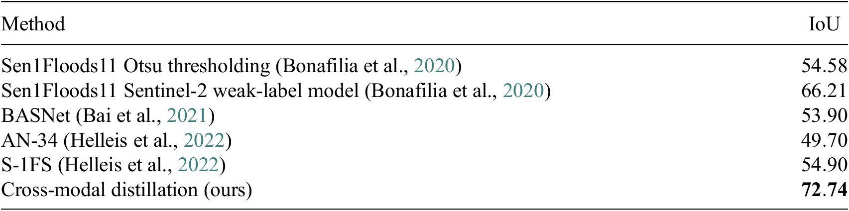
From Table 4, we can see that our method outperforms Sen1Floods11 (Bonafilia et al., Reference Bonafilia, Tellman, Anderson and Issenberg2020) weak-label baseline by an absolute margin of 6.53% IoU. In Table 4, Sen1Floods11 weak-label baseline uses FCNN (Long et al., Reference Long, Shelhamer and Darrell2015) architecture with ResNet 50 (He et al., Reference He, Zhang, Ren and Sun2016) encoder backbone. Similarly, AN-34 (Helleis et al., Reference Helleis, Wieland, Krullikowski, Martinis and Plank2022) and S-1FS (Helleis et al., Reference Helleis, Wieland, Krullikowski, Martinis and Plank2022) use UNet-based (Ronneberger et al., Reference Ronneberger, Fischer and Brox2015) encoder–decoder architecture with ResNet 34 as the base encoder. BASNet (Bai et al., Reference Bai, Wu, Yang, Yu, Zhao, Liu, Yang, Mas and Koshimura2021) also uses ResNet encoder with skip connection in the decoder. We used DeepLab v3+ in our model over FCNN and UNet as DeepLab v3+ uses atrous convolutions to capture multi-scale contextual information.
5. Sensitivity analysis
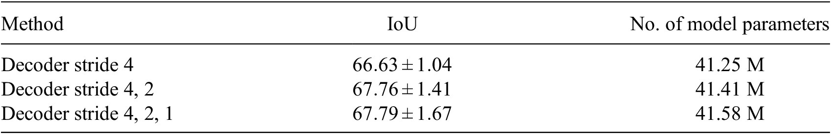
5.1. Effect of decoder stride
In the DeepLabv3+ (Chen et al., Reference Chen, Zhu, Papandreou, Schroff and Adam2018) architecture, an input image is first passed to an encoder to generate semantically meaningful features at different scales. The final encoder output feature has an output stride of 16, that is, the input image is downsampled by a factor of 16. This feature is then passed through atrous spatial pyramid pooling (ASPP) layers and the decoder to produce the output logits. The decoder processes the encoder features at a list of multiple strides—a hyper-parameter that can be tuned to refine the output segmentation masks. At each stride, the low-level features from the encoder having the same spatial dimensions are concatenated with the decoder features to process them further. The smallest stride in the list refers to the final ratio of the original input image size with the final logits size. The final logits are then bi-linearly upsampled to the required input size. Table 5 presents the effect of the decoder stride on the validation split results. It can be seen that as we concatenate finer resolutions features from the encoder with the decoder features, the number of model parameters increase and the results improve. However, the rate of improvement declines. We decided to go with a decoder stride of (4, 2) as there were diminishing gains with a decoder stride of (4, 2, 1) and a small increase in the number of model parameters.
Table 5. Validation split results for decoder stride comparison on Sen1Floods11 hand-labeled split
Note. The numbers show the aggregated mean and standard deviation of IoU from five runs.
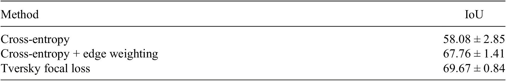
5.2. Effect of loss function
We also show the comparison of different loss function in Table 6 on the validation split. We experimented with cross-entropy loss and Tversky focal loss (Abraham and Khan, Reference Abraham and Khan2019). Tversky focal loss is a modification of the Dice coefficient (Milletari et al., Reference Milletari, Navab and Ahmadi2016) used for evaluating the overlap between the predicted segmentation mask and the ground truth mask. A limitation of Dice coefficient is that it equally weighs the false positives and the false negatives in the loss. This results in high precision and low recall. Tversky focal loss improves this by allowing flexibility to weigh the false positives and the false negatives. As a result, it is commonly used to handle class imbalance in the dataset and achieve a much better trade-off between precision and recall.
Table 6. Validation split results for loss comparison on Sen1Floods11 hand-labeled split
Note. The numbers show the aggregated mean and standard deviation of IoU from five runs.
As can be seen from Table 6 that vanilla cross-entropy loss performs poorly. On the other hand, cross-entropy with edge weighting improves vanilla cross-entropy loss by $ 9.68\% $
IoU. Also Tversky focal loss outperforms edge-weighted cross-entropy loss by a margin of
$ 9.68\% $
IoU. Also Tversky focal loss outperforms edge-weighted cross-entropy loss by a margin of $ 1.91\% $
IoU. However, we observed that the water class probability outputs with Tversky focal loss were not calibrated. A neural network is said to be calibrated if its output confidence is equal to the probability of it being correct. This means that if the network assigns a high confidence to a prediction, it should indeed be correct with a high probability. For example, a perfectly calibrated neural network would assign a probability of
$ 1.91\% $
IoU. However, we observed that the water class probability outputs with Tversky focal loss were not calibrated. A neural network is said to be calibrated if its output confidence is equal to the probability of it being correct. This means that if the network assigns a high confidence to a prediction, it should indeed be correct with a high probability. For example, a perfectly calibrated neural network would assign a probability of $ 0.8 $
to an example if it is indeed correct
$ 0.8 $
to an example if it is indeed correct $ 80\% $
of the time. Compared to Tversky loss that classifies both correct and incorrect water pixels with high confidence, cross-entropy loss produced a more calibrated output. We decided to go with cross-entropy loss as a better calibrated output helps in interpreting the reliability of the networks predictions and making informed decisions based on those probabilities.
$ 80\% $
of the time. Compared to Tversky loss that classifies both correct and incorrect water pixels with high confidence, cross-entropy loss produced a more calibrated output. We decided to go with cross-entropy loss as a better calibrated output helps in interpreting the reliability of the networks predictions and making informed decisions based on those probabilities.
6. Conclusion
To improve the performance of flood mapping models, we proposed a simple cross-modal distillation framework to effectively leverage large amounts of unlabeled and paired satellite data and a limited amount of high-quality hand-labeled data. We distill knowledge from a teacher trained on the hand-labeled images using the more informative modality as input. This helped us generate more accurate labels for the student network as compared to weak labels created by a simple thresholding technique. The student network trained this way outperforms both the supervised hand-label and weak-label baselines. Some of the model’s limitations are evident in its inability to accurately predict thin rivers and handle ambiguities in Sentinel-1 data. These challenges may arise due to the model’s reliance on a single timestamp image, which lacks temporal context and leads to difficulties in distinguishing certain features. Hence, a promising avenue for future research would be to include temporal imagery to improve performance. Another future direction we would like to explore is the effect of size of unlabeled data on model performance. This will provide insights into the cost-effectiveness of acquiring more unlabeled data.
Acknowledgments
We would like to thank Yotam Gigi and John Platt for reviewing the paper and providing invaluable feedback.
Author contribution
Conceptualization: S.G. and V.G.; Data curation: B.F., S.T., G.D., and A.G.R.; Data visualization: S.G. and B.F.; Methodology: S.G., V.B., and V.G.; Writing original draft: S.G. and V.G. All authors approved the final submitted draft.
Competing interest
The authors declare no competing interests exist.
Data availability statement
Sen1Floods11 dataset that supports the findings of this study are available on GitHub at https://github.com/cloudtostreet/Sen1Floods11. Floods208 dataset—the additional flooding events imagery dataset, cannot be released for confidentiality reasons.
Ethics statement
The research meets all ethical guidelines, including adherence to the legal requirements of the study country.
Funding statement
This work received no specific grant from any funding agency, commercial, or not-for-profit sectors.


 Open access