Chapter Overview

Water flows from high to low potential as described by Darcy’s law. The Richards equation combines Darcy’s law with principles of water conservation to calculate water movement in soil. Particular variants of the Richards equation are the mixed-form, head-based, and moisture-based equations. Water movement is determined by hydraulic conductivity and matric potential, both of which vary with soil moisture and additionally depend on soil texture. This chapter reviews soil moisture and the Richards equation. Numerical solutions are given for the various forms of the equation.

8.1 Introduction

The region of soil between the ground surface and the water table is known as the unsaturated, or vadose, zone, and the water held in this zone is called soil moisture (Figure 8.1). The water content of the vadose zone is dynamic, ranging from saturation in the upper soil layers near the surface during infiltration to nearly dry in prolonged absence of rainfall as plant roots extract water during transpiration. The vertical profile of soil water is a particularly important determinant of land–atmosphere coupling. A dry surface layer develops in the absence of rainfall, and this dry layer impedes soil evaporation. Conversely, plant roots can extend deep in the soil to sustain transpiration during dry periods. Below the vadose zone lies saturated groundwater, and soil moisture also controls the fluxes of water between the vadose zone and groundwater.

Figure 8.1 Water flows in a soil column extending from the ground surface to the water table.

The first models of the land surface used in climate simulations ignored the complexity of the hydrologic cycle and instead abstracted it using the bucket analogy in which soil is treated as a bucket that fills from precipitation, empties from evapotranspiration, or spills over as runoff as described in Chapter 7. In fact, however, storage of water and its movement in soil is much more complex. When soil is wet, water is loosely held in soil and quickly drains due to the force of gravity. When soil is dry, water movement becomes more difficult, and at some critical amount the water is strongly bound to soil particles and can no longer be removed. Figure 8.2 illustrates the dynamics of water movement during infiltration into initially dry soil. A distinct wetting front moves progressively downward over time. The upper soil becomes saturated with water while the deeper soil remains dry. In the sandy soil shown in Figure 8.2, the upper 50–60 cm become saturated after 42 minutes (0.7 h). This dynamics is explained from physical principles using Darcy’s law and the Richards equation.

Figure 8.2 Soil water movement during infiltration into sand. Shown are the initial moisture profile (θ = 0.1$\theta =0.1$) and profiles in increments of 0.1 h.

Adapted from Haverkamp et al. (Reference Haverkamp, Vauclin, Touma, Wierenga and Vachaud1977)

8.2 Measures of Soil Moisture

A typical soil consists of solid particles of varying size and shape that are interconnected by pores. Water completely fills these pores when the soil is saturated, or the pores consist mainly of air when the soil is dry. Most conditions in the field are in-between, and soil is a mix of solid particles, water, and air (Figure 8.3). The bulk density of a soil ρ_b${\rho }_b$ (kg m^–3) is the mass of soil solids per volume of soil so that

${\rho }_b=\frac{\text{mass of solids}}{\text{volume of soil}}=\frac{m_s}{V}.$(8.1)

The bulk volume of soil consists of the total volume of solids and pore space (V = V_s + V_p$V=V_s+V_p$). The particle density ρ_s${\rho }_s$ (kg m^–3) is the mass of soil solids per volume of soil solids whereby

${\rho }_s=\frac{\text{mass of solids}}{\text{volume of solids}}=\frac{m_s}{V_s}.$(8.2)

If a volume of soil 10 cm × 10 cm × 10 cm has a dry mass of 1.325 kg, its bulk density is 1325 kg m^–3. If the pore space comprises one-half of this volume, V_s = 0.5V$V_s=0.5V$, and the particle density is 2650 kg m^–3. A typical particle density is, in fact, 2650 kg m^–3. The fraction of the soil volume comprising pores, known as porosity, is (V − V_s)/V$\left(V-V_s\right)/V$. When saturated, water fills all the pores so that porosity is also the volumetric water content at saturation θ_sat${\theta }_{\mathrm{sat}}$. Porosity is calculated from bulk density and particle density by

${\theta }_{\mathrm{sat}}=1-\frac{{\rho }_b}{{\rho }_s}.$(8.3)

Figure 8.3 Depiction of soil with total volume V$V$ comprising soil solids V_s$V_s$, water V_w$V_w$, and air V_a$V_a$. The total volume of pore space is V_p = V_w + V_a$V_p=V_w+V_a$. The total soil mass consists of soil solids with mass m_s$m_s$ and water with mass m_w$m_w$.

The amount of water can be measured by volume (m³ H₂O) and equivalently by mass per area (kg H₂O m^–2) or depth (m H₂O). These are related by the density of water (ρ_wat = 1000${\rho }_{\mathrm{wat}}=1000$kg m^–3) so that mass per area = depth × density$\text{mass}\mathrm{per}\text{area}=\text{depth}\times \text{density}$. One kilogram of water spread over an area of one square meter (1 kg m^–2) is equivalent to a depth of 1 mm and a volume of 0.001 m³. A common measure of soil moisture is volumetric water content (m³ H₂O m^–3 soil). Volumetric water content is

$\theta =\frac{\text{volume of water}}{\text{volume of soil}}=\frac{V_w}{V}.$(8.4)

Volumetric water content is also the depth of water per unit depth of soil. A soil with thickness Δz$\Delta z$ m contains θ Δz$\theta \Delta z$ m of water. The mass of water per area W$W$ (kg m^–2) in a volume of soil with volumetric water content θ$\theta$ is

Another measure of soil moisture is gravimetric (mass) water content (kg H₂O kg^–1 dry soil). Gravimetric water content is

${\theta }_m=\frac{\text{mass of water}}{\text{mass of}\mathrm{dry}\text{soil}}=\frac{m_w}{m_s}.$(8.6)

Volumetric water content is related to gravimetric water content by the density of water and the bulk density of soil as

$\theta ={\theta }_m\frac{{\rho }_b}{{\rho }_{\mathrm{wat}}}.$(8.7)

Another measure is the effective saturation, which is defined as the soil moisture θ$\theta$ above some residual amount θ_res${\theta }_{\mathrm{res}}$ relative that at saturation:

$S_e=\frac{\theta -{\theta }_{\mathrm{res}}}{{\theta }_{\mathrm{sat}}-{\theta }_{\mathrm{res}}}.$(8.8)

Table 8.1 provides example calculations for these various measures of soil moisture.

Table 8.1 Various measures of soil water for a volume of soil with dimensions 10 cm × 10 cm × 10 cm that has a mass of 1.7 kg when wet, 1.45 kg when dry, and particle density ρ_s = 2650${\rho }_s=2650$ kg m^–3

Quantity	Amount
Mass of water	mw = 1.7 kg − 1.45 kg = 0.25$m_w=1.7\mathrm{kg}-1.45\mathrm{kg}=0.25$kg
Mass of soil solids	ms = 1.45$m_s=1.45$kg
Bulk volume of soil	V = 0.1 m × 0.1 m × 0.1 m = 0.001$V=0.1m\times 0.1m\times 0.1m=0.001$m3
Bulk density	ρb = ms/V = 1450${\rho }_b=m_s/V=1450$ kg m–3
Porosity	θsat = 1 − ρb/ρs = 0.453${\theta }_{\mathrm{sat}}=1-{\rho }_b/{\rho }_s=0.453$
Volume of water	Vw = mw/ρwat = 0.00025$V_w=m_w/{\rho }_{\mathrm{wat}}=0.00025$ m3
Gravimetric water content	θm = mw/ms = 0.172${\theta }_m=m_w/m_s=0.172$ kg kg–1
Volumetric water content	θ = Vw/V = θmρb/ρwat = 0.25$\theta =V_w/V={\theta }_m{\rho }_b/{\rho }_{\mathrm{wat}}=0.25$ m3 m–3
Water content relative to saturation	θ/θsat = 0.552$\theta /{\theta }_{\mathrm{sat}}=0.552$
Depth of water	θ Δz = 0.25 × 0.1 m = 0.025$\theta \Delta z=0.25\times 0.1m=0.025$ m
Mass of water per area	$W=\frac{0.25\mathrm{kg}}{0.1m\times 0.1m}=\theta \Delta z{\rho }_{\mathrm{wat}}=25$ kg m–2

8.3 Matric Potential and Hydraulic Conductivity

Water is tightly held by the surfaces of soil particles. This creates a negative pressure, or suction, called matric potential ψ$\psi$ that binds water to the soil. (The symbol h$h$ is commonly used in soil science and hydrology to denote this as pressure head.) The matric force is positive when represented as suction and negative when given as potential. Matric potential varies with soil moisture. Relatively weak suction is exerted on water when soil is saturated (matric potential is high), but suction increases sharply (matric potential decreases) as soil becomes drier and strong forces bind water in small pores. This relationship between ψ$\psi$ and θ$\theta$ is quite nonlinear and varies depending on soil texture (Figure 8.4). Water is loosely held in sandy soils (low suction) and tightly held in clay soils (high suction).

Figure 8.4 Water content in relation to matric potential given here as suction (−ψ$-\psi$).

Shown is the van Genuchten (Reference van Genuchten1980) θ(ψ)$\theta \left(\psi \right)$relationship for Berino loamy fine sand (θ_res = 0.0286${\theta }_{\mathrm{res}}=0.0286$, θ_sat = 0.3658${\theta }_{\mathrm{sat}}=0.3658$, α = 0.028$\alpha =0.028$ cm^–1, n = 2.239$n=2.239$) and Glendale silty clay loam (θ_res = 0.106${\theta }_{\mathrm{res}}=0.106$, θ_sat = 0.4686${\theta }_{\mathrm{sat}}=0.4686$, α = 0.0104$\alpha =0.0104$ cm^–1, n = 1.3954$n=1.3954$) from Hills et al. (Reference Hills, Hudson, Porro and Wierenga1989).

The dependence between ψ$\psi$ and θ$\theta$ is referred to as the soil moisture retention curve and is described mathematically by equations that relate θ$\theta$ to ψ$\psi$ or, equivalently, ψ$\psi$ to θ$\theta$, denoted θ(ψ)$\theta \left(\psi \right)$ or ψ(θ)$\psi \left(\theta \right)$, respectively. Table 8.2 gives three common relationships. Brooks and Corey (Reference Brooks and Corey1964, Reference Brooks and Corey1966) related ψ$\psi$ to the effective saturation S_e$S_e$. In this equation, ψ_b${\psi }_b$ and c$c$ are empirical parameters used to fit the data; ψ_b${\psi }_b$ is the air entry water potential and is the value of ψ$\psi$ at which S_e = 1$S_e=1$; c$c$ is referred to as the pore-size distribution index. Campbell (Reference Campbell1974) proposed a similar relationship but with θ_res = 0${\theta }_{\mathrm{res}}=0$, in which case ψ_b${\psi }_b$ can be thought of as the matric potential at saturation. Van Genuchten (Reference van Genuchten1980) developed another widely used soil moisture retention curve. In this relationship, the empirical parameter α$\alpha$ is the inverse of the air entry potential (α = 1/ ∣ ψ_b∣$\alpha =1/\mid {\psi }_b\mid$), and n$n$ is the pore-size distribution index.

Table 8.2 Soil moisture retention and hydraulic conductivity functions

θ(ψ)$\theta \left(\psi \right)$	K(θ)$K\left(\theta \right)$
(a) Brooks and Corey (Reference Brooks and Corey1964, Reference Brooks and Corey1966)
$S_e=\frac{\theta -{\theta }_{\mathrm{res}}}{{\theta }_{\mathrm{sat}}-{\theta }_{\mathrm{res}}}={\left(\frac{\psi }{{\psi }_b}\right)}^{-c}$	$K=K_{\mathrm{sat}}{S}_e^{2/c+3}$
$\frac{\mathrm{d\theta }}{\mathrm{d\psi }}=\frac{-c\left({\theta }_{\mathrm{sat}}-{\theta }_{\mathrm{res}}\right)}{{\psi }_b}{\left(\frac{\psi }{{\psi }_b}\right)}^{-c-1}$	$\frac{\mathrm{dK}}{\mathrm{d\theta }}=\frac{K_{\mathrm{sat}}}{{\theta }_{\mathrm{sat}}-{\theta }_{\mathrm{res}}}\left(2/c+3\right)S_e^{2/c+2}$
(b) Campbell (Reference Campbell1974)
$\frac{\theta }{{\theta }_{\mathrm{sat}}}={\left(\frac{\psi }{{\psi }_{\mathrm{sat}}}\right)}^{-1/b}$	$K=K_{\mathrm{sat}}{\left(\frac{\theta }{{\theta }_{\mathrm{sat}}}\right)}^{2b+3}$
$\frac{\mathrm{d\theta }}{\mathrm{d\psi }}=\frac{-{\theta }_{\mathrm{sat}}}{b{\psi }_{\mathrm{sat}}}{\left(\frac{\psi }{{\psi }_{\mathrm{sat}}}\right)}^{-1/b-1}$	$\frac{\mathrm{dK}}{\mathrm{d\theta }}=\frac{K_{\mathrm{sat}}\left(2b+3\right)}{{\theta }_{\mathrm{sat}}}{\left(\frac{\theta }{{\theta }_{\mathrm{sat}}}\right)}^{2b+2}$
(c) van Genuchten (Reference van Genuchten1980)
$S_e=\frac{\theta -{\theta }_{\mathrm{res}}}{{\theta }_{\mathrm{sat}}-{\theta }_{\mathrm{res}}}={\left(1+{\left(\alpha \left(\psi \right)\right)}^n\right)}^{-m}$, m = 1 − 1/n$m=1-1/n$	$K=K_{\mathrm{sat}}{S}_e^{1/2}{\left(1-{\left(1-S_e^{1/m}\right)}^m\right)}^2$
$\frac{\mathrm{d\theta }}{\mathrm{d\psi }}=\frac{\mathrm{\alpha mn}\left({\theta }_{\mathrm{sat}}-{\theta }_{\mathrm{res}}\right){\left(\alpha \left(\psi \right)\right)}^{n-1}}{{\left(1+{\left(\alpha \left(\psi \right)\right)}^n\right)}^{m+1}}$	$\frac{\mathrm{dK}}{\mathrm{d\theta }}=\frac{K_{\mathrm{sat}}}{\left({\theta }_{\mathrm{sat}}-{\theta }_{\mathrm{res}}\right)}\left(\frac{f^2}{2S_e^{1/2}}+\frac{2S_e^{1/m-1/2}f}{{\left(1-S_e^{1/m}\right)}^{1-m}}\right)$, $f=1-{\left(1-S_e^{1/m}\right)}^m$

Note: (a) S_e = 1$S_e=1$ and K = K_sat$K=K_{\mathrm{sat}}$ for ψ>ψ_b$\psi >{\psi }_b$. (b) θ/θ_sat = 1$\theta /{\theta }_{\mathrm{sat}}=1$ and K = K_sat$K=K_{\mathrm{sat}}$ for ψ>ψ_sat$\psi >{\psi }_{\mathrm{sat}}$. (c) S_e = 1$S_e=1$ and K = K_sat$K=K_{\mathrm{sat}}$ for ψ>0$\psi >0$.

Parameter values vary depending on soil texture, and various so-called pedotransfer functions relate hydraulic parameters to discrete texture classes or as continuous functions of sand, clay, or other soil properties. The Brooks and Corey (Reference Brooks and Corey1964, Reference Brooks and Corey1966) parameters, for example, can be related to sand, clay, and porosity (Rawls and Brakensiek Reference Rawls, Brakensiek, Jones and Ward1985; Rawls et al. Reference Rawls, Ahuja, Brakensiek, Shirmohammadi and Maidment1993). Clapp and Hornberger (Reference Clapp and Hornberger1978) estimated parameters for various soil texture classes using the Campbell (Reference Campbell1974) relationship, and Cosby et al. (Reference Cosby, Hornberger, Clapp and Ginn1984) subsequently related θ_sat${\theta }_{\mathrm{sat}}$, ψ_sat${\psi }_{\mathrm{sat}}$, and b$b$ to the sand and clay content of soil. The van Genuchten (Reference van Genuchten1980) parameters can be difficult to estimate (Carsel and Parrish Reference Carsel and Parrish1988; Leij et al. Reference Leij, Alves, van Genuchten and Williams1996; Schaap et al. Reference Schaap, Leij and van Genuchten1998, Reference Schaap, Leij and van Genuchten2001). Table 8.3 gives representative values for soil texture classes.

Water held in soil is subjected to two forces, or potentials. The force of gravity pulls water downward, denoted as gravitational potential. Gravitational potential is the height z$z$ above some arbitrary reference height. The second force is the matric potential, which holds water to the soil particles. The total potential, also known as hydraulic head, is ψ + z$\psi +z$, and this is the work per unit weight required to move an amount of water at some elevation and matric potential to another position in the soil with a different potential. Soil water potential as used in this chapter has the units of energy per unit weight and has the dimension of length (m):

$\frac{\text{energy}}{\text{weight}}=\frac{J}{N}=\frac{N\cdot m}{N}=m$

Other units for potential are energy per unit mass (J kg^–1) or energy per unit volume (J m^–3), and this latter expression is also the units of pressure (Pa). Soil water potential is converted from m to J kg^–1 by multiplying by gravitational acceleration g$g$ and to J m^–3 by multiplying by ρ_watg${\rho }_{\mathrm{wat}}g$:

A wet soil with a matric potential of –0.01 MPa has a suction of approximately 1000 mm; a dry soil with –1.5 MPa has a suction of approximately 150 m.

Hydraulic conductivity governs the rate of water flow for a unit gradient in potential. Hydraulic conductivity decreases sharply as soil becomes drier because suction increases and because the pore space filled with water becomes smaller and discontinuous. This relationship is nonlinear and varies with soil texture (Figure 8.5). Sandy soil has a higher conductivity than clay soil. The relationship between K$K$ and θ$\theta$ is not independent of the relationship between θ$\theta$ and ψ$\psi$, and the derivation of K(θ)$K\left(\theta \right)$ requires an expression for θ(ψ)$\theta \left(\psi \right)$ (Figure 8.4). This expression is given in terms of the effective saturation S_e$S_e$, or θ/θ_sat$\theta /{\theta }_{\mathrm{sat}}$ in the Campbell (Reference Campbell1974) equation, so that hydraulic conductivity can be equivalently expressed as K(ψ)$K\left(\psi \right)$. The expressions for hydraulic conductivity also require K_sat$K_{\mathrm{sat}}$, the hydraulic conductivity at saturation. The term $S_e^{1/2}$ in the van Genuchten (Reference van Genuchten1980) equation for hydraulic conductivity is a common form, but the exponent can vary (Schaap et al. Reference Schaap, Leij and van Genuchten2001). Better fit to data can be achieved by replacing K_sat$K_{\mathrm{sat}}$ with a curve fitting parameter K₀$K_0$, but this has a value that is usually less than K_sat$K_{\mathrm{sat}}$ so that K(θ)≠K_sat$K\left(\theta \right)\ne K_{\mathrm{sat}}$ at θ_sat${\theta }_{\mathrm{sat}}$ (Schaap et al. Reference Schaap, Leij and van Genuchten2001).

Figure 8.5 Hydraulic conductivity in relation to water content. Shown is the van Genuchten (Reference van Genuchten1980) K(θ)$K\left(\theta \right)$relationship for Berino loamy fine sand and Glendale silty clay loam. Parameter values are as in Figure 8.4 and K_sat$K_{\mathrm{sat}}$= 22.54 and 0.55 cm h^–1, respectively.

(Hills et al. Reference Hills, Hudson, Porro and Wierenga1989)

8.4 Richards Equation

Darcy’s law describes water flow. In the vertical dimension, the rate of water movement is

$Q=-K\left(\theta \right)\frac{\partial \left(\psi +z\right)}{\partial z}=-K\left(\theta \right)\left(\frac{\partial \psi }{\partial z}+1\right)=-K\left(\theta \right)\frac{\partial \psi }{\partial z}-K\left(\theta \right).$(8.9)

This is a form of Fick’s law and relates the rate of flow to the product of the hydraulic conductivity and the vertical gradient in water potential. The flux Q$Q$ is the volume of water (m³) flowing through a unit cross-sectional area (m²) per unit time (s) and has the dimensions length per time (m s^–1). Hydraulic conductivity has the same units, and K(θ)$K\left(\theta \right)$ denotes that hydraulic conductivity depends on soil moisture. The total potential ψ + z$\psi +z$ has dimensions of length (m). It governs water movement so that water flows from high to low potential. The vertical depth z$z$ is taken as positive in the upward direction so that z = 0$z=0$ is the ground surface and z < 0$z<0$ is the elevation relative to the surface with greater depth into the soil. The matric potential has values ψ < 0$\psi <0$ for unsaturated soil and ψ ≥ 0$\psi \ge 0$ for saturated soil. The negative sign in (8.9) ensures that downward water flow is negative and upward flow is positive.

The flow of water given by Darcy’s law depends strongly on soil moisture. The dominant force causing water to move in a wet soil is the gravitation potential. Water near the surface has a higher gravitational potential than water deeper in the soil, and because water flows from high potential to low potential, it flows downward from the force of gravity. This is given by z$z$ in (8.9), which is the height relative to the ground surface. In drier soils, matric potential decreases, and the adsorptive force binding water to soil particles generally exceeds the gravitational force pulling water downward. This reduces the rate of water flow. The lower hydraulic conductivity in dry soils also restricts water movement.

An equation for the time rate of change in soil moisture is obtained from principles of conservation similar to that for soil temperature. Consider a volume of soil with horizontal area ΔxΔy$\Delta x\Delta y$ and thickness Δz$\Delta z$ and in which water flows only in the vertical dimension (Figure 8.6). The mass flux of water (kg s^–1) entering the soil across the cross-sectional area ΔxΔy$\Delta x\Delta y$ is ρ_watQ_inΔxΔy${\rho }_{\mathrm{wat}}{Q}_{\text{in}}\Delta x\Delta y$, and the flux out of the soil is similarly ρ_watQ_outΔxΔy${\rho }_{\mathrm{wat}}{Q}_{\mathrm{out}}\Delta x\Delta y$. Conservation requires that the difference between the flux of water into and out of the soil equals the rate of change in water storage. The mass of water in the soil volume is ρ_watθΔxΔyΔz${\rho }_{\mathrm{wat}}\theta \Delta x\Delta y\Delta z$ so that the change in soil water over the time interval Δt$\Delta t$ is

${\rho }_{\mathrm{wat}}\frac{\Delta \theta }{\Delta t}\Delta x\Delta y\Delta z=-{\rho }_{\mathrm{wat}}\left(Q_{\text{in}}-Q_{\mathrm{out}}\right)\Delta x\Delta y$(8.10)

and

$\frac{\Delta \theta }{\Delta t}=-\frac{\Delta Q}{\Delta z}.$(8.11)

Equation (8.11) is the continuity equation for water, with the left-hand side the change in water storage and the right-hand side the flux divergence.

Figure 8.6 Water balance for a soil volume with the fluxes Q_in$Q_{\text{in}}$ entering the volume and Q_out$Q_{\mathrm{out}}$ exiting the volume.

In the notation of calculus, the continuity equation is

$\frac{\partial \theta }{\partial t}=-\frac{\partial Q}{\partial z},$(8.12)

and substituting Darcy’s law for Q$Q$ gives

$\frac{\partial \theta }{\partial t}=\frac{\partial }{\partial z}\left(K\left(\theta \right)\frac{\partial \psi }{\partial z}+K\left(\theta \right)\right)=\frac{\partial }{\partial z}\left(K\left(\theta \right)\frac{\partial \psi }{\partial z}\right)+\frac{\partial K}{\partial z}.$(8.13)

This is the Richards equation and describes the movement of water in an unsaturated porous medium (Richards Reference Richards1931). Equation (8.13) is called the mixed-form equation because it includes the time rate of change in θ$\theta$ on the left-hand side and the vertical gradient in ψ$\psi$ on the right-hand side. Other forms of the Richards equation use the dependence between ψ$\psi$ and θ$\theta$ to express the equation in terms of only one unknown variable. The head-based, or ψ$\psi$-based, form transforms the storage term on the left-hand side of the equation from θ$\theta$ to ψ$\psi$ so that ψ$\psi$ is the dependent variable. This uses the chain rule to expand ∂θ/∂t$\partial \theta /\partial t$ as

$\frac{\partial \theta }{\partial t}=\frac{\mathrm{d\theta }}{\mathrm{d\psi }}\frac{\partial \psi }{\partial t}=C\left(\psi \right)\frac{\partial \psi }{\partial t},$(8.14)

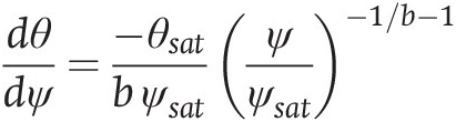
in which C(ψ) = dθ/dψ$C\left(\psi \right)=\mathrm{d\theta }/\mathrm{d\psi }$ is known as the specific moisture capacity (m^–1) and is the slope of the soil moisture retention curve. Then (8.13) is rewritten as

$C\left(\psi \right)\frac{\partial \psi }{\partial t}=\frac{\partial }{\partial z}\left(K\left(\theta \right)\frac{\partial \psi }{\partial z}\right)+\frac{\partial K}{\partial z}.$(8.15)

The ψ$\psi$-based form is applicable for unsaturated and saturated conditions and provides a continuous equation for water flow in the vadose zone and for groundwater. However, it is not mass conserving because the specific moisture capacity dθ/dψ$\mathrm{d\theta }/\mathrm{d\psi }$ that appears in the storage term itself depends on ψ$\psi$ and so is not constant over a discrete time interval during which ψ$\psi$ changes value (Milly Reference Milly1985; Celia et al. Reference Celia, Bouloutas and Zarba1990). Whereas (8.14) is mathematically correct, its temporal discretization over some time interval Δt$\Delta t$ (as required in numerical methods) is not equivalent. The moisture-based, or θ$\theta$-based, equation uses θ$\theta$ as the dependent variable with

$\frac{\partial \theta }{\partial t}=\frac{\partial }{\partial z}\left(D\left(\theta \right)\frac{\partial \theta }{\partial z}\right)+\frac{\partial K}{\partial z},$(8.16)

in which D(θ) = K(θ)/C(ψ)$D\left(\theta \right)=K\left(\theta \right)/C\left(\psi \right)$ is referred to as the hydraulic diffusivity (m² s^–1). In this equation, the specific moisture capacity appears within the spatial derivative. The θ$\theta$-based form is mass conserving but is restricted to the unsaturated zone because soil moisture does not vary within a saturated porous medium (soil moisture is bounded by 0 ≤ θ ≤ θ_sat$0\le \theta \le {\theta }_{\mathrm{sat}}$) whereas pressure head does vary. Furthermore, the equation is restricted to homogenous soils because θ$\theta$ is not continuous across soil layers with different θ(ψ)$\theta \left(\psi \right)$ relationships. As a result, soils in which texture varies with depth have discontinuous vertical profiles of θ$\theta$, whereas ψ$\psi$ is continuous even in inhomogeneous soils.

The Richards equation requires relationships for K(θ)$K\left(\theta \right)$ and θ(ψ)$\theta \left(\psi \right)$. Analytical solutions are difficult to obtain because these relationships are highly nonlinear. Instead, numerical methods are used, which requires first writing the finite difference approximation of the partial differential equation and then linearizing the nonlinear terms involving K(θ)$K\left(\theta \right)$ and C(ψ)$C\left(\psi \right)$. The accuracy of the solution very much depends on the details of the numerical methods, the form of the Richards equation, and the size of the time step and grid spacing. The literature on numerical methods to solve the Richards equation is enormous. The next two sections provide an introduction to this literature with the caveat that many more numerical techniques are available and the merits of particular methods are still being debated.

8.5 Finite Difference Approximation

The finite difference approximation for the Richards equation represents the soil as a network of discrete nodal points that vary in space and time similar to that for soil temperature. In doing so, it is necessary to remember that hydraulic conductivity is not constant but, rather, varies with depth depending on soil moisture so that the mixed-form equation is expanded as

$\frac{\partial \theta }{\partial t}=K\left(\theta \right)\frac{{\partial }^2\psi }{\partial z^2}+\frac{\partial K}{\partial z}\frac{\partial \psi }{\partial z}+\frac{\partial K}{\partial z}.$(8.17)

For reasons of numerical stability similar to soil temperature, (8.17) is solved using an implicit time discretization in which the spatial derivatives ∂K/∂z$\partial K/\partial z$, ∂ψ/∂z$\partial \psi /\partial z$, and ∂²ψ/∂z²${\partial }^2\psi /\partial z^2$ are written numerically using a central difference approximation at time n + 1$n+1$, and the time derivative uses a backward difference approximation at n + 1$n+1$ (Appendix A4). For a vertical grid with discrete layers each equally spaced at a distance Δz$\Delta z$ and with z$z$ positive in the upward direction so that layer i$i$ is above layer i + 1$i+1$, the numerical form of (8.17) is

$\frac{{\theta }_i^{n+1}-{\theta }_i^n}{\Delta t}=\frac{K_i^{n+1}}{\Delta z^2}\left({\psi }_{i-1}^{n+1}-2{\psi }_i^{n+1}+{\psi }_{i+1}^{n+1}\right)+\left(\frac{K_{i-1}^{n+1}-K_{i+1}^{n+1}}{2\Delta z}\right)\left(\frac{{\psi }_{i-1}^{n+1}-{\psi }_{i+1}^{n+1}}{2\Delta z}\right)+\frac{K_{i-1}^{n+1}-K_{i+1}^{n+1}}{2\Delta z}.$(8.18)

This is an implicit solution in which θ$\theta$ and ψ$\psi$ are expressed at n + 1$n+1$, and K$K$ is similarly evaluated with θ$\theta$ at n + 1$n+1$. Rearranging terms gives an equivalent form in which

$\frac{{\theta }_i^{n+1}-{\theta }_i^n}{\Delta t}=\frac{K_{i-1/2}^{n+1}}{\Delta z^2}\left({\psi }_{i-1}^{n+1}-{\psi }_i^{n+1}\right)-\frac{K_{i+1/2}^{n+1}}{\Delta z^2}\left({\psi }_i^{n+1}-{\psi }_{i+1}^{n+1}\right)+\frac{K_{i-1/2}^{n+1}-K_{i+1/2}^{n+1}}{\Delta z},$(8.19)

with

$K_{i\pm 1/2}^{n+1}=K_i^{n+1}\pm \frac{K_{i+1}^{n+1}-K_{i-1}^{n+1}}{4}.$(8.20)

The ψ$\psi$-based form of the equation is obtained by replacing the left-hand side of (8.19) with $C_i^{n+1}\left({\psi }_i^{n+1}-{\psi }_i^n\right)/\Delta t$.

A more general derivation of (8.19) is obtained by considering the mass balance of a soil layer. Figure 8.7 depicts the soil profile in a cell-centered grid of N$N$ discrete layers similar to that used for soil temperature. Soil layer i$i$ has a thickness Δz_i$\Delta z_i$. Water content θ_i${\theta }_i$, matric potential ψ_i${\psi }_i$, and hydraulic conductivity K_i$K_i$ are defined at the center of the layer at depth z_i$z_i$ and are uniform over the layer. Depth decreases in the downward direction from the surface so that z₀ = 0$z_0=0$ denotes the surface and z_i + 1 < z_i$z_{i+1}<z_i$ (i.e., depths are negative distances from the surface). The flux of water Q_i$Q_i$ between adjacent layers i$i$ and i + 1$i+1$ depends on the hydraulic conductivities of the two layers. The hydraulic conductivity K_i + 1/2$K_{i+1/2}$ replaces the vertically varying hydraulic conductivities in the two adjacent layers with an effective conductivity for an equivalent homogenous medium so that the flux Q_i$Q_i$ is

$Q_i=-\frac{K_{i+1/2}}{\Delta z_{i+1/2}}\left({\psi }_i-{\psi }_{i+1}\right)-K_{i+1/2},$(8.21)

with Δz_i + 1/2 = z_i − z_i + 1$\Delta z_{i+1/2}=z_i-z_{i+1}$ the distance between nodes i$i$ and i + 1$i+1$. The flux Q_i − 1$Q_{i-1}$ at the top of soil layer i$i$ is similarly

$Q_{i-1}=-\frac{K_{i-1/2}}{\Delta z_{i-1/2}}\left({\psi }_{i-1}-{\psi }_i\right)-K_{i-1/2},$(8.22)

and Δz_i − 1/2 = z_i − 1 − z_i$\Delta z_{i-1/2}=z_{i-1}-z_i$. With fluxes expressed for time n + 1$n+1$, the mass balance for soil layer i$i$ is

$\frac{{\theta }_i^{n+1}-{\theta }_i^n}{\Delta t}=-\frac{Q_{i-1}^{n+1}-Q_i^{n+1}}{\Delta z_i}$(8.23)

so that

$\frac{\Delta z_i}{\Delta t}\left({\theta }_i^{n+1}-{\theta }_i^n\right)=\frac{K_{i-1/2}^{n+1}}{\Delta z_{i-1/2}}\left({\psi }_{i-1}^{n+1}-{\psi }_i^{n+1}\right)-\frac{K_{i+1/2}^{n+1}}{\Delta z_{i+1/2}}\left({\psi }_i^{n+1}-{\psi }_{i+1}^{n+1}\right)+K_{i-1/2}^{n+1}-K_{i+1/2}^{n+1}.$(8.24)

For constant soil layer thickness, this is equivalent to (8.19).

Figure 8.7 Multilayer soil water flow in a cell-centered grid oriented such that i = 1$i=1$ is the top soil layer at the surface, and i = N$i=N$ is the bottom soil layer. Each layer has a thickness Δz_i$\Delta z_i$. The depth z_i − 1/2$z_{i-1/2}$ is the interface between adjacent layers i − 1$i-1$ and i$i$, and z_i + 1/2$z_{i+1/2}$ is the interface between i$i$ and i + 1$i+1$. Depths are negative distances from the surface so that Δz_i = z_i − 1/2 − z_i + 1/2$\Delta z_i=z_{i-1/2}-z_{i+1/2}$ (i.e., z_i + 1/2 = z_i − 1/2 − Δz_i$z_{i+1/2}=z_{i-1/2}-\Delta z_i$). The depth z_i$z_i$ is defined at the center of layer i$i$ so that z_i = (z_i − 1/2 + z_i + 1/2)/2$z_i=\left(z_{i-1/2}+z_{i+1/2}\right)/2$. Δz_i ± 1/2$\Delta z_{i\pm 1/2}$ is the grid spacing between i$i$ and i ± 1$i\pm 1$. Water content θ_i${\theta }_i$, matric potential ψ_i${\psi }_i$, and hydraulic conductivity K_i$K_i$ are defined at the center of layer i$i$ at depth z_i$z_i$ and are uniform over the layer. An effective hydraulic conductivity K_i ± 1/2$K_{i\pm 1/2}$ is defined at the interface between soil layers at depth z_i ± 1/2$z_{i\pm 1/2}$. Shown are (a) the first soil layer (i = 1$i=1$); (b) layers 1 < i < N$1<i<N$ depicted generally as three soil layers denoted i − 1$i-1$, i$i$, and i + 1$i+1$; and (c) the bottom soil layer (i = N$i=N$). The surface matric potential ψ₀${\psi }_0$ or the flux Q₀$Q_0$ provide the upper soil boundary condition, and the lower boundary condition at the bottom of the soil is ψ_N + 1${\psi }_{N+1}$ or gravitational drainage Q_N$Q_N$.

Equation (8.24) describes the water balance of soil layers 1 < i < N$1<i<N$. Special equations are needed for the top (i = 1$i=1$) and bottom (i = N$i=N$) layers to account for boundary conditions. Boundary conditions at the surface are specified in terms of ψ₀${\psi }_0$ (Dirichlet boundary condition) or as a flux of water Q₀$Q_0$ into the soil (Neumann boundary condition). With the surface value ψ₀${\psi }_0$ specified, (8.24) is still valid, in which case the corresponding flux of water into the soil is

$Q_0^{n+1}=-\frac{K_{1/2}^{n+1}}{\Delta z_{1/2}}\left({\psi }_0^{n+1}-{\psi }_1^{n+1}\right)-K_{1/2}^{n+1}.$(8.25)

Alternatively, Q₀$Q_0$ can be directly specified as the boundary condition (e.g., as an infiltration rate; negative into the soil), in which case the water balance for layer i = 1$i=1$ is

$\frac{\Delta z_i}{\Delta t}\left({\theta }_i^{n+1}-{\theta }_i^n\right)=-Q_0^{n+1}-\frac{K_{i+1/2}^{n+1}}{\Delta z_{i+1/2}}\left({\psi }_i^{n+1}-{\psi }_{i+1}^{n+1}\right)-K_{i+1/2}^{n+1}.$(8.26)

The lower boundary condition at the bottom of the soil column can similarly be specified in terms of ψ$\psi$ or as a flux of water. When given as the matric potential ψ_N + 1${\psi }_{N+1}$, the corresponding flux of water draining out of the soil column is

$Q_N^{n+1}=-\frac{K_{N+1/2}^{n+1}}{\Delta z_{N+1/2}}\left({\psi }_N^{n+1}-{\psi }_{N+1}^{n+1}\right)-K_{N+1/2}^{n+1}.$(8.27)

A common flux boundary condition specifies free drainage at the bottom of the soil column in which Q_N =  − K_N$Q_N=-K_N$. This is referred to as a unit hydraulic gradient because ∂ψ/∂z = 0$\partial \psi /\partial z=0$ in the Darcian flux. The water balance of layer i = N$i=N$ is then

$\frac{\Delta z_i}{\Delta t}\left({\theta }_i^{n+1}-{\theta }_i^n\right)=\frac{K_{i-1/2}^{n+1}}{\Delta z_{i-1/2}}\left({\psi }_{i-1}^{n+1}-{\psi }_i^{n+1}\right)+K_{i-1/2}^{n+1}-K_i^{n+1}.$(8.28)

Alternatively, the soil column can be coupled with a groundwater model to allow for the influence of water table dynamics on soil moisture. The total change in water in the soil column equals the net flux into the soil so that conservation is given by

$\sum _{i=1}^N\left({\theta }_i^{n+1}-{\theta }_i^n\right)\Delta z_i=\left(Q_N^{n+1}-Q_0^{n+1}\right)\Delta t.$(8.29)

Equation (8.20) defines the effective conductivity K_i ± 1/2$K_{i\pm 1/2}$ from the central difference approximation for (∂K/∂z)(∂ψ/∂z)$\left(\partial K/\partial z\right)\left(\partial \psi /\partial z\right)$. Hydraulic conductivity can differ substantially between layers because of vertical gradients in soil moisture (e.g., during infiltration into a dry soil). The equation used to represent the effective conductivity affects the accuracy of the numerical solution, and other expressions can be used for K_i ± 1/2$K_{i\pm 1/2}$ (Haverkamp and Vauclin Reference Haverkamp and Vauclin1979; Warrick Reference Warrick1991, Reference Warrick2003). The effective conductivity can be defined as the arithmetic mean of the adjacent nodal conductivities in which

Another expression is the geometric mean whereby

The harmonic mean is the reciprocal of the arithmetic mean of the reciprocals with

$K_{i\pm 1/2}=\frac{1}{0.5\left(K_i^{-1}+K_{i\pm 1}^{-1}\right)}=\frac{2K_i{K}_{i\pm 1}}{K_i+K_{i\pm 1}}.$(8.32)

This latter equation is similar to (5.16) for the effective thermal conductivity and is obtained for constant Δz$\Delta z$ from continuity of flow across the interface so that the flux of water from depth z_i$z_i$ to z_i + 1/2$z_{i+1/2}$ equals the flux from z_i + 1/2$z_{i+1/2}$ to z_i + 1$z_{i+1}$. While the harmonic mean ensures continuity of fluxes at the interface, it is weighted towards the lower value of the two hydraulic conductivities and is the smallest of the three means. The arithmetic mean has the largest value, and the geometric mean has an intermediate value. The arithmetic mean is commonly used – e.g., as in the numerical solutions of Haverkamp et al. (Reference Haverkamp, Vauclin, Touma, Wierenga and Vachaud1977) and Celia et al. (Reference Celia, Bouloutas and Zarba1990).

The numerical form of the ψ$\psi$-based Richards equation is similar to (5.18) for soil temperature. For a soil with N$N$ layers, this is a tridiagonal system of N$N$ equations with N$N$ unknown values of ψ$\psi$ at time n + 1$n+1$. This is more obvious by rewriting the finite difference approximation of the mixed-form equation given by (8.24) in the ψ$\psi$-based form and rearranging terms to get

$-\frac{K_{i-1/2}^{n+1}}{\Delta z_{i-1/2}}{\psi }_{i-1}^{n+1}+\left(\frac{C_i^{n+1}\Delta z_i}{\Delta t}+\frac{K_{i-1/2}^{n+1}}{\Delta z_{i-1/2}}+\frac{K_{i+1/2}^{n+1}}{\Delta z_{i+1/2}}\right){\psi }_i^{n+1}-\frac{K_{i+1/2}^{n+1}}{\Delta z_{i+1/2}}{\psi }_{i+1}^{n+1}=\frac{C_i^{n+1}\Delta z_i}{\Delta t}{\psi }_i^n+K_{i-1/2}^{n+1}-K_{i+1/2}^{n+1}.$(8.33)

A general form for this equation is

$a_i{\psi }_{i-1}^{n+1}+b_i{\psi }_i^{n+1}+c_i{\psi }_{i+1}^{n+1}=d_i,$(8.34)

or, in matrix notation (Appendix A6),

$\left(\begin{array}{cccccc}{b}_1& c_1& 0& 0& 0& 0\\ a_2& b_2& c_2& 0& 0& 0\\ 0& a_3& b_3& c_3& 0& 0\\ 0& 0& \ddots & \ddots & \ddots & 0\\ 0& 0& 0& a_{N-1}& b_{N-1}& c_{N-1}\\ 0& 0& 0& 0& a_N& b_N\end{array}\right)\times \left(\begin{array}{c}{\psi }_1^{n+1}\\ {\psi }_2^{n+1}\\ {\psi }_3^{n+1}\\ ⋮\\ {\psi }_{N-1}^{n+1}\\ {\psi }_N^{n+1}\end{array}\right)=\left(\begin{array}{c}{d}_1\\ d_2\\ d_3\\ ⋮\\ d_{N-1}\\ d_N\end{array}\right),$(8.35)

in which the matrix elements a$a$, b$b$, c$c$, and d$d$ are evident from (8.33), with special values for i = 1$i=1$ and i = N$i=N$ to account for boundary conditions (Table 8.4).

Table 8.4 Tridiagonal terms for the ψ$\psi$-based Richards equation

Layer	ai$a_i$	bi$b_i$	ci$c_i$	di$d_i$
i = 1$i=1$	0	$\frac{C_i^{n+1}\Delta z_i}{\Delta t}+\frac{K_{1/2}^{n+1}}{\Delta z_{1/2}}-c_i$	$-\frac{K_{i+1/2}^{n+1}}{\Delta z_{i+1/2}}$	$\frac{C_i^{n+1}\Delta z_i}{\Delta t}{\psi }_i^n+\frac{K_{1/2}^{n+1}}{\Delta z_{1/2}}{\psi }_0^{n+1}+K_{1/2}^{n+1}-K_{i+1/2}^{n+1}$
1 < i < N$1<i<N$	$-\frac{K_{i-1/2}^{n+1}}{\Delta z_{i-1/2}}$	$\frac{C_i^{n+1}\Delta z_i}{\Delta t}-a_i-c_i$	$-\frac{K_{i+1/2}^{n+1}}{\Delta z_{i+1/2}}$	$\frac{C_i^{n+1}\Delta z_i}{\Delta t}{\psi }_i^n+K_{i-1/2}^{n+1}-K_{i+1/2}^{n+1}$
i = N$i=N$	$-\frac{K_{i-1/2}^{n+1}}{\Delta z_{i-1/2}}$	$\frac{C_i^{n+1}\Delta z_i}{\Delta t}-a_i$	0	$\frac{C_i^{n+1}\Delta z_i}{\Delta t}{\psi }_i^n+K_{i-1/2}^{n+1}-K_N^{n+1}$

Note: Boundary conditions are ${\psi }_0^{n+1}$ for the first layer (i = 1$i=1$) and free drainage for the bottom layer (i = N$i=N$).

However, whereas soil temperature uses a linear equation, (8.33) is a nonlinear equation for ψ$\psi$ because of the complex dependence of K$K$ and C$C$ on ψ$\psi$. This nonlinearity is evident when these terms are replaced with their various expressions given in Table 8.2. An additional complexity is that ψ$\psi$ at n + 1$n+1$ also appears on the right-hand side of (8.33) through K$K$ and C$C$. Solving a nonlinear equation is challenging, and solving the system of nonlinear equations required to represent N$N$ soil layers is especially challenging. The solution requires linearizing (8.33) with respect to ψ$\psi$ through various numerical methods. One simple linearization uses values of K$K$ and C$C$ obtained at the preceding time step (at time n$n$ rather than n + 1$n+1$). This is an implicit solution for ψ$\psi$ but with explicit linearization of K$K$ and C$C$ (Haverkamp et al. Reference Haverkamp, Vauclin, Touma, Wierenga and Vachaud1977).

A better numerical technique is the predictor–corrector method. This is a two-step solution that solves the Richards equation twice. The predictor step uses explicit linearization to solve for ψ$\psi$ over one-half a full time step (Δt/2$\Delta t/2$) at time n + 1/2$n+1/2$ with K$K$ and C$C$ from time n$n$. The resulting values for ψ$\psi$ are used to evaluate K$K$ and C$C$ at n + 1/2$n+1/2$, and the corrector step uses these to obtain ψ$\psi$ over the full time step (Δt$\Delta t$) at n + 1$n+1$. The method can be applied to the ψ$\psi$-based Richard equations (Haverkamp et al. Reference Haverkamp, Vauclin, Touma, Wierenga and Vachaud1977) or the θ$\theta$-based equation (Hornberger and Wiberg Reference Hornberger and Wiberg2005). These implementations use an implicit solution for the predictor step and the Crank–Nicolson method (Appendix A4) for the corrector step. The predictor equation for ψ$\psi$ at n + 1/2$n+1/2$ is