


1. Introduction
The difficulties in developing hyperbolic two-fluid models for disperse multiphase flows has been reviewed by Lhuillier, Chang & Theofanous (Reference Lhuillier, Chang and Theofanous2013). Many of the models that have been proposed in the literature suffer from being mathematically ill posed (see Drew & Passman Reference Drew and Passman1998; Vazquez-Gonzalez, Llor & Fochesato Reference Vazquez-Gonzalez, Llor and Fochesato2016, for other discussions of this topic), most notably when the Archimedes force is included. Mathematically, well posedness of nonlinear multiphase flow models implies hyperbolicity of the underlying Cauchy problem (Métivier Reference Métivier2005). In practice, numerical simulations with non-hyperbolic two-fluid models diverge under grid refinement due to the complex eigenvalues in the continuum limit (see, e.g. Ndjinga Reference Ndjinga2007; Kumbaro & Ndjinga Reference Kumbaro and Ndjinga2011). To solve this problem, ad hoc correction terms have been added to make the models well posed (see, e.g. Panicker, Passalacqua & Fox Reference Panicker, Passalacqua and Fox2018). In particular, some authors have resorted to neglecting the Archimedes force (see, e.g. Hank, Saurel & Le Metayer Reference Hank, Saurel and Le Metayer2011), which is the root cause of non-hyperbolicity. For bubbly flows the Archimedes force is of critical importance when buoyancy effects are present.
Starting from a kinetic-theory description, Fox (Reference Fox2019) developed a hyperbolic two-fluid model for gas–particle flows that neglects added-mass effects (as well as inelastic collisions and viscous effects). The model equations were derived starting from the Boltzmann–Enskog kinetic theory for a binary hard-sphere mixture. A closure for the particle-pair distribution functions was introduced to account for the Archimedes force in the limit where one particle diameter is much smaller than the other. However, because the closure for the particle-pair distribution function only accounts for mean gradients, it cannot capture the higher-order correlations needed for added mass. The system of velocity moment equations was truncated at second order, and the unclosed collisional source terms were closed using an isotropic Gaussian (Maxwellian) distribution (Levermore & Morokoff Reference Levermore and Morokoff1996; Vié, Doisneau & Massot Reference Vié, Doisneau and Massot2015). Then, by employing Sturm's theorem (Sturm Reference Sturm1829), it was demonstrated that the resulting two-fluid model is hyperbolic for physically realistic values of the model parameters. In comparison to other two-fluid models, novel contributions to the pressure tensor and energy flux (which appear in closed form) arise and play a key role in ensuring hyperbolicity when fluid and particle material densities satisfy  $\rho _f \ll \rho _p$. Here, we employ the same model formulation, extended to account for the added mass from particle wakes and pseudo-turbulence, to compressible fluid–particle flows with a slip velocity due, e.g. to buoyancy.
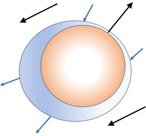
Our treatment of added mass is similar to Cook & Harlow (Reference Cook and Harlow1984) (see appendix A for more details), but generalized to a compressible fluid and a non-constant added-mass function. The latter is required to handle flows wherein the particle-phase volume fraction varies significantly. In our model and in the model of Cook & Harlow (Reference Cook and Harlow1984), mathematical objectivity is ensured, unlike in other formulations (e.g. Drew, Cheng & Lahey Reference Drew, Cheng and Lahey1979; Massoudi Reference Massoudi2002). In the context of kinetic theory, the approach of Cook & Harlow (Reference Cook and Harlow1984) where the added mass moves with the particle velocity allows us to simply redefine the particle properties without changing the basic form of the kinetic equation governing the velocity distribution function (Fox Reference Fox2019). Nonetheless, because the fluid in the particle wake is not fixed, but exchanges with the bulk fluid, mass transfer must be included in the kinetic equation to model the convective mass-transfer process. Here, a simple model is employed that depends on a mass-exchange function  $S_a$. (See figure 1 for details.) Because the mass-transfer model involves neither spatial nor temporal derivatives, its form does not affect the hyperbolicity of the two-fluid model.

Figure 1. Schematic of a particle with its added volume of fluid (i.e. the wake of the particle). The fluid in the wake exchanges mass with the external fluid at a net rate determined by  $S_a$. The total particle volume, moving with velocity $\boldsymbol {u}_p$, is $V_p^{\star }$ with sub-volume $V_p$ having material density $\rho _p$ and added volume $V_a$ having material density $\rho _f$. The external fluid with material density $\rho _f$ and moving with velocity $\boldsymbol {u}_f$, has volume $V_f^{\star } = V - V_p^{\star }$. The mass of the particle is $m_p = \rho _p V_p + \rho _f V_a$. In terms of the volume fractions, $m_p = ( \rho _p \alpha _p + \rho _f \alpha _a ) V = \rho _e \alpha _p^{\star } V$ where $\rho _e$ is the effective density of the particle with its added mass and $\alpha _p^{\star } = \alpha _p + \alpha _a$. Thus, the added volume of fluid moving with the particle velocity is $\alpha _a V$, and the added mass is $\rho _f \alpha _a V$. The added-volume fraction must satisfy $0 \le \alpha _a \le \alpha _f$ so it is convenient to define an added-mass function $c_m$ by $\alpha _a = c_m \alpha _p \alpha _f$. As the added volume is usually associated with particle wakes, $c_m$ can depend on the particle Reynolds number $Re_p$, the particle-phase volume fraction, and other dimensionless parameters needed to describe the flow. In the limit $\alpha _p \to 1$, all of the fluid can be assumed to move with the particle so that $c_m \to 1$; however, this is not required for hyperbolicity.
From a kinetic-theory perspective, the added mass of fluid on a particle can be accounted for by defining a particle's volume and mass to include the fluid moving with the particle (Marchisio & Fox Reference Marchisio and Fox2013), i.e. the fluid in the particle wake (Moore & Balachandar Reference Moore and Balachandar2019). The total particle mass  $m_p$ is then employed in the kinetic-theory expressions for the velocity moments. This procedure introduces two volume fractions, namely $\alpha _p$ and $\alpha _p^{\star } = \alpha _p + \alpha _a$. The former is the usual volume fraction of the particle phase, while the latter includes the volume of the fluid moving with the particles. Naturally, $\alpha _p^{\star } \ge \alpha _p$ and the corresponding fluid-phase volume fractions are $\alpha _f^{\star }=1-\alpha _p^{\star }$ and $\alpha _f=1-\alpha _p$, respectively. A similar decomposition of the fluid-phase variables is used by Osnes et al. (Reference Osnes, Vartdal, Omang and Reif2019) to define a modified slip velocity ( $\boldsymbol {u}_{free}= \alpha _f \boldsymbol {u}_{fp} / \alpha _f^{\star }$) in supersonic gas–particle flows. Using arguments similar to those of Risso (Reference Risso2018) for bubbly flows, these authors also reported that the pseudo-turbulence in the streamwise direction is well approximated by $\alpha _a u_{fp}^2 / \alpha _f^{\star }$, and for fixed $\alpha _p$ show that $\alpha _a$ decreases with increasing $Re_p$ (Osnes et al. Reference Osnes, Vartdal, Omang and Reif2020).
For the analysis of hyperbolicity, it is convenient to introduce an added-mass function  $c_m$ defined such that $\alpha _a =c_m \alpha _p \alpha _f$. In principle, $c_m$ can be a function of the slip velocity between the two phases (i.e. of the particle Reynolds number $Re_p=\rho _f d_p u_{fp}/ \mu _f$ where $d_p$ is the particle diameter and $\mu _f$ is fluid viscosity), the density ratio $Z=\rho _p/\rho _f$, and the volume fraction $\alpha _p$ (Zuber Reference Zuber1964; Sangani, Zhang & Prosperetti Reference Sangani, Zhang and Prosperetti1991; Zhang & Prosperetti Reference Zhang and Prosperetti1994). However, in the dilute limit, Odar & Hamilton (Reference Odar and Hamilton1964) found experimentally that $c_m$ depends only on the acceleration number $Ac = u_{fp}^2/(a d_p)$ where $a$ is the magnitude of the particle acceleration, which we approximation below using the drag force. Unless $c_m=0$, the phase velocities found from the kinetic-theory derivation will not be equal to those found from volume averaging unless added mass is accounted for in the latter. Nevertheless, the kinetic-theory derivation leads to conservation laws in the form of hyperbolic equations. This has advantages over a formulation where the virtual mass is treated as an interphase force when solving the two-fluid model numerically.
Finally, because the added mass can vary from location to location in the flow, mass transfer between the bulk fluid and the added-mass fluid (i.e. the particle wake) must be accounted for in the model. This is done by introducing an added-mass exchange rate  $S_a$. The exchange of mass between the bulk fluid and added mass also induces an exchange of momentum and kinetic energy, which depends on the direction of the mass exchange. The bulk-fluid momentum is $\rho _f \alpha _f^{\star } \boldsymbol {u}_f$, while that of the added-mass fluid is $\rho _f \alpha _a \boldsymbol {u}_p$. Concerning the total energy, for the particle phase it is defined by
 \begin{equation} \rho_e \alpha_p^{\star} E_p = \rho_e \alpha_p^{\star} \left( \frac{\varTheta_p}{\gamma_p - 1} + \frac{1}{2} u_p^2 \right) , \end{equation}
where  $\gamma _p = 5/3$ for hard spheres, $\varTheta _p$ is the granular temperature and $\rho _e \alpha _p^{\star } = \rho _p \alpha _p + \rho _f \alpha _a$ defines $\rho _e$. For simplicity, in (1.1) the internal energy associated with the solid phase and the added mass is neglected. Otherwise, an additional scalar transport equation would be required, which does not change the hyperbolicity of the system (Houim & Oran Reference Houim and Oran2016). For the bulk fluid, the total energy is defined by
 \begin{equation} \rho_f \alpha_f^{\star} E_f = \rho_f \alpha_f^{\star} \left( \frac{\varTheta_f}{\gamma_f - 1} + \frac{1}{2} u_f^2 + k_f \right), \end{equation}
where  $\gamma _f$ is the fluid specific heat ratio, $\varTheta _f$ is the fluid temperature and $k_f$ is the pseudo-turbulent kinetic energy (PTKE). In the two-fluid model, the momentum-exchange contribution is equal to $S_a \boldsymbol {u}_f$ or $S_a \boldsymbol {u}_p$, and the energy-exchange contribution to $S_a (u_f^2/2 + k_f)$ or $S_a E_p$, depending on the sign of $S_a$. The asymmetry in the energy exchange from the bulk fluid to the particle wake results from neglecting the internal energy in (1.1). In the compressible two-fluid model, (1.1) and (1.2) are used to find the temperatures $\varTheta _p$ and $\varTheta _f$ given the total energies $E_p$ and $E_f$, respectively. In the stiffened-gas model used for the fluid, $\varTheta _f$ must be initialized such that the fluid pressure $p_f$ is positive.
2. Two-fluid model for compressible flows
2.1. Governing equations
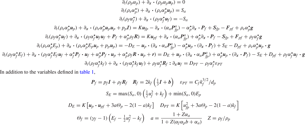
The governing equations for mono-disperse particles in a compressible fluid with added mass, but neglecting PTKE, are given in table 1. If PTKE is taken into account (Shallcross, Fox & Capecelatro Reference Shallcross, Fox and Capecelatro2020), the model has the form given in table 2. We should point out that in the balance equation for  $k_f$ the part of the source term $D_{PT}$ due to drag is $K u_{fp}^2$, which is the same as the correlated part of the source term for total energy $D_E$. Physically, this implies that viscous losses are ignored during the exchange process such that drag transfers energy to $k_f$ from the particle phase, which is subsequently dissipated to uncorrelated energy by $\varepsilon _{PT}$. The accuracy of this assumption is likely to depend on the particle Reynolds number, i.e. it will be more accurate for high $Re_p$ where the particle wakes are turbulent. In practice, this difference can be accounted for by multiplying $K u_{fp}^2$ in $D_{PT}$ (but not in $D_E$) by a damping factor dependent on $Re_p$. Doing so, it may be possible to reduce the Mach number dependence of $C_f$ observed in Shallcross et al. (Reference Shallcross, Fox and Capecelatro2020).
Table 1. Compressible two-fluid model for particles in a fluid modelled as a stiffened gas. Typical values of the specific heat ratios are  $\gamma _f = 29/4$ and $\gamma _p = {5}/{3}$, and for the stiffened-gas constant $p^o_f = 10^8\ \textrm {kg}\,\textrm {m}^{-1}\,\textrm {s}^{2}$: $C_D$ is the drag coefficient that depends on the particle Reynolds number $Re_p$, fluid Mach number and volume fraction; and $\boldsymbol {g}$ is gravity. The default added-mass function is $c_m^{\star } = \min (1 + 2 \alpha _p , 2)/2$.

Table 2. Compressible two-fluid model for particles in a fluid modelled as a stiffened gas with a transport equation for PTKE  $k_f$. The pseudo-turbulence tensor $\boldsymbol {R}_f$ arises due to the finite size of the particles and $\boldsymbol {b}$ is the PTKE anisotropy tensor (Tenneti, Garg & Subramaniam Reference Tenneti, Garg and Subramaniam2011). The model for $a$ is based on the asymptotic behaviours for $\rho _f=0$ and $\rho _p=0$. The parameter $b$ fixes the ratio $3 \varTheta _p / 2 k_f$ when $\rho _p=0$, and direct numerical simulation data (Tavanashad et al. Reference Tavanashad, Passalacqua, Fox and Subramaniam2019) suggest that $b=0.365$. The constant $C_f$ is order one and fixes the magnitude of $k_f$ in spatially homogeneous flow (Shallcross et al. Reference Shallcross, Fox and Capecelatro2020). An alternative is to use a transport equation for $\varepsilon _{PT}$ to account for the integral length scale of PTKE in lieu of $d_p$.
In prior work (Fox Reference Fox2019), it has been demonstrated that for an ideal gas ( $\gamma _f=5/3$) with material densities such that $\rho _p \gg \rho _f$ and $\alpha _a=0$ the two-fluid model in table 1 is hyperbolic for physically relevant values of the parameters. In this work, we mainly consider the opposite case with $\rho _p \ll \rho _f$ where the fluid phase is described by the stiffened-gas model (Harlow & Amsden Reference Harlow and Amsden1971; Saurel & Abgrall Reference Saurel and Abgrall1999). For a pure fluid, the latter gives an equation of state of the form $p_f = \rho _f \varTheta _f - p_f^o$ where the constant $p_f^o$ is used to set the speed of sound in the fluid phase. For example, water can be simulated with $p_f^o \approx 2225\ \textrm {MPa}$. The fluid temperature $\varTheta _f$ $(\textrm {m}^{2}\,\textrm {s}^{-2})$ is found from the fluid energy $E_f$ as shown in table 1, and must be large enough that $p_f > 0$. In this work, we will use a stiffened-gas model of the form
 \begin{equation} p_f = \rho_f \varTheta_f - \gamma_f (\gamma_f -1) p^o_f \frac{\alpha_f}{\alpha_f^{\star}} . \end{equation}
The actual value of  $p_f^o$ is not important as long as the speed of sound is much larger than the other characteristic velocities (or eigenvalues) of the system. The factor $\alpha _f / \alpha _f^{\star }$ has been added to handle the limiting case where $\alpha _f \to 0$ (i.e. densely packed particles), for which this ratio diverges. Other forms of the stiffened-gas model are possible, and the factor is not needed for more dilute systems where the disperse-phase eigenvalues remain well separated from those of the fluid phase. For the disperse (i.e. particle) phase, the radial distribution function $g_0$ controls the speed of sound as $\alpha _f$ approaches zero. For example, if $g_0$ is replaced with unity, the particle-phase speed of sound is weakly dependent on $\alpha _p$. Here, to analysis the hyperbolicity of the two-fluid model, we use a form for $g_0$ applicable to non-deformable spheres, but other forms can be used as long as $1 \le g_0$. Furthermore, replacing $\alpha _f / \alpha _f^{\star }$ with $g_0$ in (2.1) will not change the conclusions drawn in § 3 concerning the hyperbolicity of the two-fluid models.
The kinetic-theory model derived in Fox (Reference Fox2019) made specific assumptions concerning the two-particle distribution function that may be inaccurate for non-ideal gases and liquids. Specifically, the terms involving  $\boldsymbol {R}$ and $\boldsymbol {r}$ in table 1 are exact for hard-sphere collisions (i.e. $\gamma _f = \gamma _p = 5/3$), but their definition in a stiffened gas is less obvious (e.g. should they depend on both $\gamma _f$ and $\gamma _p$?). Thus, in our analysis of the hyperbolicity of the two-fluid model in § 3 we also consider a simplified version where these terms are neglected in the fluid phase. Nonetheless, because the particle-phase pressure tensor $\boldsymbol {P}_p$ includes an added-mass contribution involving $\boldsymbol {R}$, one can argue that $\boldsymbol {P}_p$ has its origins in the kinetic-theory description. In fact, in § 3 we show that the eigenvalues of the one-dimensional (1-D) model are mainly determined by the choice of $\boldsymbol {P}_p$ and $p_f$, with $\boldsymbol {R}$ and $\boldsymbol {r}$ in the fluid phase only slightly changing the eigenvalues (while making the hyperbolicity analysis more complicated). Thus, from the standpoint of applications to real systems, the simplified model may offer a good compromise between computation cost and model accuracy. However, one would also need to account for inelastic collisions, particle-phase viscosity, as well as other effects (see, e.g. Abbas et al. Reference Abbas, Climent, Parmentier and Simonin2010) in most applications, none of which affect the hyperbolicity.
2.2. Added-mass model
In addition to the fluid drag with coefficient  $K$, the models in tables 1 and 2 include the buoyancy force, compressibility, lift and added mass. Compressibility and lift are contained in the exchange force $\boldsymbol {F}_{pf}$ (Fox Reference Fox2019). The added-mass contribution is treated differently than in most other two-fluid models where balance equations are written for each phase with a virtual-mass force. Instead, here the phases are defined by their velocities $\boldsymbol {u}_p$ and $\boldsymbol {u}_f$, and the added mass moves with the particle velocity $\boldsymbol {u}_p$ (see discussion in Cook & Harlow Reference Cook and Harlow1984). For example, the mass per unit volume of the fluid phase moving with velocity $\boldsymbol {u}_f$ is $\rho _f \alpha _f^{\star } = \rho _f ( \alpha _f - \alpha _a )$. Note that
 \begin{equation} \rho_f \alpha_f^{\star} + \rho_e \alpha_p^{\star} = \rho_f \alpha_f +\rho_p \alpha_p, \end{equation}
 so that the mixture density is independent of  $\alpha _a$. The various volume fractions appearing in the model are related by
 \begin{equation} \alpha_f^{\star} = \alpha_f - \alpha_a \quad \alpha_p^{\star} = \alpha_p + \alpha_a \quad \alpha_p + \alpha_f = 1. \end{equation}
Given the conserved variables  $(X_1,X_2,X_3)=(\rho _p \alpha _p , \rho _e \alpha _p^{\star }, \rho _f \alpha _f^{\star })$ and the particle density $\rho _p$, the volume fractions and fluid density are uniquely determined by
 \begin{equation} (\alpha_p, \rho_f, \alpha_a) = \left( \frac{X_1}{\rho_p} , \frac{X_3+X_2-X_1}{\alpha_f}, \frac{X_2 - X_1}{\rho_f} \right) . \end{equation}
Hereinafter, we define the variable  $c_m$ such that $\alpha _a = c_m \alpha _f \alpha _p$, which is a convenient form to enforce the upper limit on $\alpha _a$.
Although its definition is not required to analyse the hyperbolicity, the added-mass exchange rate will be approximated by a linear relaxation model
 \begin{equation} S_a = \frac{\rho_f \alpha_f \alpha_p}{\tau_a} ( c_m^{\star} - c_m ), \end{equation}
with time scale
 \begin{equation} \tau_a = \frac{4 d_p^2 \alpha_f^{\star}}{3 \nu_f C_D Re_p \alpha_f} . \end{equation}
Physically,  $\tau _a$ is the time scale characterizing the expansion/contraction/formation of particle wakes. For example, when a particle moves from a region with large $\alpha _p$ to one with small $\alpha _p$ (i.e. to larger spacing between particles), $c_m$ will be smaller than $c_m^{\star }$. Thus, the wake will grow by entraining fluid with velocity $\boldsymbol {u}_f$ and kinetic energy $u_f^2/2 + k_f$. The time scale in (2.6) is meant to estimate this rate of growth and can be further refined using data from particle-resolved direct numerical simulations (PRDNS) (see, e.g. Moore & Balachandar Reference Moore and Balachandar2019).
2.3. Added-mass function
In principle, by formulating a physically accurate function for  $c_m^{\star }$, the two-fluid model will be able to account correctly for unsteady effects. For example, $c_m^{\star }$ might depend on $Ac$ (Odar & Hamilton Reference Odar and Hamilton1964), making the added mass of the particle larger when the particle acceleration is high. In this work, we are primary interested in the effect of added mass on the hyperbolicity of the two-fluid model. In this context, source terms that do not depend on space or time derivatives (such as $S_a$) have no influence on the eigenvalues of the flux matrix. Nonetheless, the added-mass function $c_m^{\star } (x)$ must have the properties $0 \le \alpha _p c_m^{\star } \le 1$ and $c_m^{\star }(0)=C_m$ where $C_m$ is the added-mass constant, which is equal to 1/2 for a spherical particle when $\alpha _p=0$ (Zuber Reference Zuber1964). In addition, one might require $c_m^{\star } (1)=1$ to force all of the fluid phase to be treated as added mass when its volume fraction approaches zero, but this is not required for hyperbolicity.
Theoretical expressions for the dependence of added mass on the particle volume fraction can be found in Sangani et al. (Reference Sangani, Zhang and Prosperetti1991); however, these expressions are valid for  $\alpha _p < 0.5$. From the hyperbolicity analysis in § 3, we find that $0.085 < c_m^{\star } < 1/ \alpha _p$, which corresponds physically to $0 < \alpha _f^{\star } < \alpha _f$. These observations suggest the use of the expression proposed by Zuber (Reference Zuber1964) (written to account for the difference between $\boldsymbol {u}_f$ and $\boldsymbol {v}_f$) of the form
 \begin{equation} c_m^{\star} = \tfrac{1}{2} \min \left( 1 + 2 \alpha_p , 2 \right) . \end{equation}
Sangani et al. (Reference Sangani, Zhang and Prosperetti1991) showed that this form is suitable for most applications (e.g., bubble and spherical particles with no-slip and free-slip boundaries); hence, it will be the default expression in the proposed two-fluid model. Nonetheless, as done in Moore & Balachandar (Reference Moore and Balachandar2019) for the velocity wakes around Lagrangian particles, PRDNS could be used to improve this model to account for the particle Reynolds number and volume fraction dependencies.
Another possible expression (which allows for direct computation of  $\alpha _p^{\star }$ versus $\alpha _p$) is the linear form
 \begin{equation} c_m^{\star} = C_m + (1-C_m) x, \end{equation}
with  $x=\alpha _p$ or $x=\alpha _p^{\star }$, and $0 \le C_m \le 2$. Based on their experimental results, Odar & Hamilton (Reference Odar and Hamilton1964) found that $C_m$ depends on the acceleration number as
 \begin{equation} C_m = 1 - \tfrac{1}{2} e^{- \beta Ac}, \end{equation}
where  $\beta \approx 3$ and the acceleration number is defined by $Ac = 4 /(3C_D)$. Thus, for very slow acceleration, $C_m=1/2$, whereas for rapid acceleration $C_m=1$. However, more recent theoretical works (e.g. Auton, Hunt & Prud'homme Reference Auton, Hunt and Prud'homme1988; Sangani et al. Reference Sangani, Zhang and Prosperetti1991; Mei & Adrian Reference Mei and Adrian1992) suggest that the decomposition of the virtual-mass and history forces used by Odar & Hamilton (Reference Odar and Hamilton1964) is not reliable, and that $C_m=1/2$ independent of $Ac$. In any case, using (2.8) and given that $\alpha _p^{\star } = \alpha _p + c_m \alpha _p (1- \alpha _p)$, at steady state where $c_m=c_m^{\star }$ with $x=\alpha _p$, the value of $\alpha _p$ is the root in the interval $[0 \ 1]$ of a cubic polynomial for $0 \le C_m \le 2$
 \begin{equation} (1-C_m) \alpha_p^3 + (2 C_m-1) \alpha_p^2 - (C_m+1) \alpha_p + \alpha_p^{\star} = 0. \end{equation}
For  $C_m = 1$, the desired root is $\alpha _f^2 = \alpha _f^{\star }$ (which also holds for (2.7) when $\alpha _f < 1/2$). For other values of $C_m$, the root can be found numerically as illustrated in figure 2.

Figure 2. Steady-state relation between  $\alpha _p$ and $\alpha _p^{\star }$ for the added-mass function $c_m^{\star }=C_m+(1-C_m)x$ with three values of $C_m$. $(a)$
$(a)$ $x=\alpha _p$. $(b)$
$(b)$ $x=\alpha _p^{\star }$. The diagonal line corresponds to $c_m^{\star }=0$. For the function in (2.7), the dependence will be the same as $C_m=1$ for $1/2 < \alpha _p$. Note that the curve for $C_m=1$ is the same for both choices of $x$.
$x$.
As previously noted, the choice of  $c_m^{\star }$ has no effect on the hyperbolicity of the two-fluid model. Notwithstanding this fact, for actual applications, it will be important to choose a functional form that accurately matches the dependence of the added mass on $\alpha _p$, etc., derived from PRDNS, experiments and theory.
2.4. Particle-phase pressure tensor
In fluid–particle flows, the particles have uncorrelated motion due to fluid-mediated interactions and direct collisions (Lhuillier et al. Reference Lhuillier, Chang and Theofanous2013). In recent PRDNS studies of bubbly flow (du Cluzeau, Bois & Toutant Reference du Cluzeau, Bois and Toutant2019; du Cluzeau et al. Reference du Cluzeau, Bois, Toutant and Martinez2020), these fluctuations are referred to as the dispersed-phase Reynolds stresses, but it is important to note that they are present in purely laminar flows (Biesheuvel & van Wijngaarden Reference Biesheuvel and van Wijngaarden1984). Indeed, in kinetic theory the magnitude of the dispersed-phase Reynolds stresses is proportional to the granular temperature  $\varTheta _p$. In du Cluzeau et al. (Reference du Cluzeau, Bois, Toutant and Martinez2020), it is found that these terms (referred to as $\boldsymbol {M}^{extra}$ and $\boldsymbol {M}^{LD}$) make a significant contribution to the dispersed-phase momentum balance. As described by these authors, in two-fluid models the corresponding flux terms in the dispersed-phase momentum balance are usually separated into ‘dispersion’ forces (proportional to $\partial _{\boldsymbol {x}} \alpha _p$) and a ‘drag’ force contributions. However, from the standpoint of examining the hyperbolicity of the two-fluid model, it is simplest to treat them as part of the momentum flux as done in this work.
Considering the effective repulsive force exerted between particles in random motion, Batchelor (Reference Batchelor1988) proposed a (1-D) particle-phase stress model written in terms of the hydrodynamic diffusivity  $D$ and the bulk mobility $B$ of the form (written in our notation)
 \begin{equation} \partial_x p_p = \partial_x \alpha_p \rho_p \varTheta_p - \frac{\rho_p D}{m_p B} \partial_x \alpha_f, \end{equation}
where  $m_p$ is the particle mass. He then used physical reasoning to argue that
 \begin{equation} \frac{\rho_p D}{m_p B} \propto \rho_f u_{fp}^2 . \end{equation}
Considering that Batchelor's model was developed for a 1-D flow with an incompressible fluid phase, it is not unreasonable to treat his dispersion term as part of the particle pressure as done in our compressible two-fluid model. From the kinetic-theory derivation (Fox Reference Fox2019), a dispersion term is also found in  $\boldsymbol {F}_{pf}$, but written in terms of $\partial _{\boldsymbol {x}} \rho _f$ and not $\partial _{\boldsymbol {x}} \alpha _f$. Thus, this dispersion term would be zero for an incompressible fluid phase. Mathematically, the dispersion term in (2.11) would appear with the opposite sign in the fluid momentum balance (i.e. it would be an interphase force), and the mixture momentum balance would only contain $p_p$.
Syamlal (Reference Syamlal2011) derived a ‘buoyant-force’ term that extends the fluid pressure in the Archimedes force to include a relative-velocity contribution of the form  $\rho _f \alpha _f \boldsymbol {u}_{fp} \otimes \boldsymbol {u}_{fp}$. Neglecting the particle pressure and considering an incompressible fluid, he demonstrates that the two-fluid model for mass and momentum with this additional force is hyperbolic. Comparing his model to the one in table 1 (and ignoring added mass), we observe that the term in the fluid-phase momentum flux involving $\boldsymbol {R}$ (which is exact from kinetic theory (Fox Reference Fox2019)) is not present, and the particle-phase pressure tensor term $\partial _{\boldsymbol {x}} \boldsymbol {\cdot } ( \alpha _a \boldsymbol {P}^a_{fp} )$ is replaced by the buoyant-force term $\alpha _p \partial _{\boldsymbol {x}} \boldsymbol {\cdot } ( \rho _f \alpha _f \boldsymbol {u}_{fp} \otimes \boldsymbol {u}_{fp} )$. In § 3.2, we find that the $\boldsymbol {R}$ contribution to the fluid-phase momentum flux is not required for hyperbolicity (and, for constant $\rho _f$, can be combined with the fluid pressure as done in § 5.2). Thus, by rewriting the buoyant-force term in the form
 \begin{equation} \alpha_p \partial_{\boldsymbol{x}} \boldsymbol{\cdot} ( \rho_f \alpha_f \boldsymbol{u}_{fp} \otimes \boldsymbol{u}_{fp} ) = \partial_{\boldsymbol{x}} \boldsymbol{\cdot} ( \rho_f \alpha_f \alpha_p \boldsymbol{u}_{fp} \otimes \boldsymbol{u}_{fp} ) - \rho_f \alpha_f (\boldsymbol{u}_{fp} \otimes \boldsymbol{u}_{fp} ) \boldsymbol{\cdot} \partial_{\boldsymbol{x}} \alpha_p , \end{equation}
it can be interpreted as a combination of a fluid-mediated particle-phase pressure tensor and a dispersion force, albeit with a negative coefficient. As we show in § 3, the fluid-mediated particle-phase pressure is essential for ensuring a hyperbolic system.
Zhang, Ma & Rauenzahn (Reference Zhang, Ma and Rauenzahn2006) and Zhang (Reference Zhang2020) derived a two-fluid formulation from a general kinetic theory accounting for long-range particle–particle interactions. A particle–fluid–particle (PFP) force of the form  $\partial _{\boldsymbol {x}} \boldsymbol {\cdot } ( \alpha _p \boldsymbol {\varSigma }_{pfp} )$, where $\boldsymbol {\varSigma }_{pfp}$ is the PFP stress, appears in their formulation. For uniform potential flow with constant $\rho _f$, Zhang (Reference Zhang2020) finds that
 \begin{equation} \alpha_p \boldsymbol{\varSigma}_{pfp} = \rho_f \left[ C_1 ( \alpha_p ) u_{fp}^2 \boldsymbol{I} + C_2 ( \alpha_p ) \boldsymbol{u}_{fp} \otimes \boldsymbol{u}_{fp} \right], \end{equation}
where  $C_1$ and $C_2$ are coefficients that can be determined numerically. Unlike in (2.13), no dispersion term arises in addition to the PFP force, nor is $\boldsymbol {\varSigma }_{pfp}$ related to the Archimedes force. Nevertheless, the stress tensor in (2.13) is a special case of (2.14) and, hence, it is reasonable to expect that the PFP force would affect favourably the hyperbolicity of the system (which depends on the trace of $\boldsymbol {\varSigma }_{pfp} \propto \rho _f u_{fp}^2$).
In kinetic theory, the dispersed-phase Reynolds stresses and fluid-mediated interactions contribute to the particle-phase pressure tensor. Thus, from a physical-modelling standpoint, an important component in the two-fluid model is the closure for this term
 \begin{equation} \boldsymbol{P}_p = p_p \boldsymbol{I} + \alpha_a \boldsymbol{P}_{fp}^a, \end{equation}
where  $p_p = \alpha _p p_p^k + \alpha _a p_f^a$ with $p_p^k = \rho _p \varTheta _p ( 1 + 4 \alpha _p^{\star } g_{0} )$, $p_f^a = \rho _f \varTheta _p ( 1 + 4 \alpha _p^{\star } g_{0} )$ and
 \begin{equation} \boldsymbol{P}_{fp}^a = \rho_f \frac{2}{3 \gamma_p} \left( \frac{1}{2} u_{fp}^2 \boldsymbol{I} + \boldsymbol{u}_{fp} \otimes \boldsymbol{u}_{fp} \right) \left( 1 + 4 \alpha_p^{\star} g_{0} \right) , \end{equation}
which is a particular form of (2.14). This model for  $\boldsymbol {P}_p$ combines the kinetic-theory dependence on $\varTheta _p$ due to uncorrelated velocity fluctuations and direct collisions when $\rho _f \ll \rho _p$ (i.e. $p_p$) with a component to describe the fluid-mediated interactions between particles that are taken to be proportional to the added mass. In other words, even when the granular temperature is null, in order to have a globally hyperbolic system we assume that a particle pressure exists due to interactions between the particles via the fluid phase (see van Wijngaarden Reference van Wijngaarden1976; Batchelor Reference Batchelor1988; Zhang et al. Reference Zhang, Ma and Rauenzahn2006; Zhang Reference Zhang2020, for detailed discussions).
In (2.16), the contribution  $1 + 4 \alpha _p^{\star } g_{0}$ with $1 \le g_0$ accounts for the excluded volume occupied by the particles. Other formulations of (2.16) are possible and will perhaps be required to capture the correct physics (e.g. when $\rho _f \approx \rho _p$ or for deformable particles such as bubbles). For example, one might consider replacing $\alpha _p^{\star } g_{0}$ with $\alpha _p g_{0}$, or changing altogether the definition of $g_0$. However, as shown in § 3, such changes will not affect the hyperbolicity of the compressible two-fluid model as long as $\gamma _p$ is not so large as to make $\boldsymbol {P}_{fp}^a$ negligible. Furthermore, in § 3 we find that with $\alpha _p=0$, the system is hyperbolic even when $c_m=0$ (i.e. $\alpha _a=0$ in (2.15)). Thus, it is possible for $\boldsymbol {P}_{fp}^a$ in (2.16) to depend linearly on $\alpha _p^{\star }$ (so that the fluid-mediated pressure depends on $\alpha _p^2$) without changing the hyperbolicity of the system. An example of this behaviour is presented in appendix B where it is shown that for an incompressible fluid the two-fluid model with $trace(\alpha _a \boldsymbol {P}_{fp}^a) \propto (\alpha _p^{\star })^2 u_{fp}^2$ is globally hyperbolic.
The tensorial form of the fluid-mediated particle pressure in (2.16), and its appearance with the opposite sign in the fluid-phase momentum balance, is motivated as follows. In the kinetic-theory derivation of Fox (Reference Fox2019), it was shown that the mixture pressure tensor has the form  $\boldsymbol {P}_{mix} = \boldsymbol {P}_1 + \boldsymbol {P}_2 + c_{12} \boldsymbol {P}_{BE}$ regardless of the size ratio between the hard spheres. The Boltzmann–Enskog contribution $\boldsymbol {P}_{BE}$ leads to the term involving $\boldsymbol {R}$ in the fluid-phase momentum balance when added mass is neglected ( $\alpha _a=0$). Biesheuvel & van Wijngaarden (Reference Biesheuvel and van Wijngaarden1984) derive a contribution to the mixture stress and liquid-phase Reynolds stresses with the same tensorial form as $\boldsymbol {R}$ based on potential flow around spherical bubbles, but neglecting particle–particle interactions. Thus, with added mass, we assume that the mixture pressure tensor remains unchanged, and share the contribution $\alpha _a \boldsymbol {P}_{fp}^a$ between the two phases. This is consistent with the kinetic-theory derivation where the particle pressures in each phase depend on the particle size ratio, while the mixture pressure does not (Fox Reference Fox2019). Finally, note that the contribution $\partial _{\boldsymbol {x}} \boldsymbol {\cdot } ( \alpha _a \boldsymbol {P}_{fp}^a )$ arises from the kinetic-theory derivation as a modification to the pressure tensors, while in the compressible two-fluid model it can be interpreted as a fluid-mediated exchange force. Finally, the parameter $\gamma _p$ in (2.16) is equal to 5/3 for a hard sphere in an ideal gas, but in general it can be used as a parameter to set the magnitude of the fluid-mediated particle pressure (i.e. $tr(\boldsymbol {P}_{fp}^a) \propto 5/(3 \gamma _p)$). On the other hand, the tensorial form of $\boldsymbol {P}_{fp}^a$ must be kept consistent with that of $\boldsymbol {R}$ as both arise due from the same term in the kinetic-theory derivation (Fox Reference Fox2019). As seen from (2.14), up to the scalar coefficients that can depend on $\alpha _p$, this tensorial form is the only one that can be formed from $\boldsymbol {u}_{fp}$ (Zhang Reference Zhang2020).
In summary, the particle-pressure tensor in (2.15) combines two limiting behaviours for the material-density ratio and it is a key modelling component for ensuring hyperbolicity when  $\rho _p \ll \rho _f$. This is consistent with Batchelor (Reference Batchelor1988) where it is also shown to have a strong effect on the linear stability of a uniform suspension. It is also consistent with the kinetic-theory derivation of Zhang et al. (Reference Zhang, Ma and Rauenzahn2006); Zhang (Reference Zhang2020) who demonstrate that an inter-species stress arises due to particle–fluid–particle interactions, which do not depend on $\varTheta _p$. Nonetheless, future research should be devoted to refining the model for $\alpha _a \boldsymbol {P}_{fp}^a$ in (2.16) to account for the $\alpha _p$ and $Re_p$ dependencies observed in PRDNS.
2.5. Limiting cases
Having previously investigated the case with  $\rho _f \ll \rho _p$ (Fox Reference Fox2019), in the remainder of this work we are particularly interested in the limiting cases with $\rho _p=0$ (i.e. the particles have zero mass) so that $\rho _e \alpha _p^{\star } = \rho _f \alpha _a$. However, we will also analyse the hyperbolicity of the complete model for selected values of the material density ratio $Z$. As is well known, the drag and body forces appearing on the right-hand sides of the model equations do not affect the eigenvalues of the two-fluid model. Hence, in § 3 we will ignore them and consider only the terms involving temporal and spatial gradients.
3. Hyperbolicity of 1-D two-fluid model
In order to determine whether the full three-dimensional (3-D) model in table 2 is hyperbolic, it suffices to consider a system with one spatial direction (see, e.g. Ndjinga Reference Ndjinga2007; Kumbaro & Ndjinga Reference Kumbaro and Ndjinga2011; Lhuillier et al. Reference Lhuillier, Chang and Theofanous2013). This approach will be followed here, starting with the 1-D model without source terms that do not involve temporal or spatial derivatives.
3.1. One-dimensional compressible two-fluid model
The 1-D model without the source terms is given in table 3, written in terms of eight independent variables
 \begin{equation} \boldsymbol{X} := \left( X_1 , X_2, X_3, X_4, X_5, X_6, X_7, X_8 \right)^t = \left(\alpha_p , \rho_e \alpha_p^{\star} / \rho_p , Z \alpha_f^{\star} , u_p, u_f, E_p, E_f, k_f \right)^t . \end{equation}
We define  $Z$ such that $\rho _f = Z \rho _p$. As $\rho _p$ is constant, it can be factored out of the model if desired. The conserved variables $( X_1, X_2, X_3)$ are related to $( \alpha _p, Z, \alpha _f^{\star } )$ by
 \begin{equation} \alpha_p = X_1 , \quad Z = \frac{X_3 + X_2 - X_1}{\alpha_f}, \quad \alpha_f^{\star} = \frac{X_3}{Z} , \end{equation}
and all other variables appearing in the momentum and energy balances can be found from these variables. In addition to the model in table 3, we will also analyse the simplified model given in table 4, which neglects the Boltzmann–Enskog fluxes (i.e.  $\boldsymbol {R}$ and $\boldsymbol {r}$ in the fluid phase) and forces (i.e. $\boldsymbol {F}_{fp}$ and $D_{fp}$) that are specific to hard-sphere mixtures (Fox Reference Fox2019).
Table 3. One-dimensional compressible two-fluid model with the densities, pressures, fluxes and forces normalized by  $\rho _p$. The reference pressure $p^{\star }_o$ is constant and has the same units as $\varTheta _f$, and $Z_0$ is the reference density ratio.
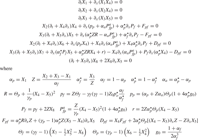
Table 4. Simplified version of 1-D compressible two-fluid model from table 3. This model is hyperbolic when the fluid-phase eigenvalues are sufficiently separated from those for the particle phase. When this is not the case, the kinetic-theory terms in the full model may be needed to achieve hyperbolicity.

Formally, the 1-D models can be rewritten as
 \begin{equation} \boldsymbol{A} ( \boldsymbol{X}) \partial_t \boldsymbol{X} + \boldsymbol{B} (\boldsymbol{X}) \partial_x \boldsymbol{X} = \boldsymbol{0}, \end{equation}
where the coefficient matrices  $\boldsymbol {A}$ and $\boldsymbol {B} := \boldsymbol {B}^* + \boldsymbol {B}_0$ yield the flux matrix $\boldsymbol {F} := \boldsymbol {A}^{-1} \boldsymbol {B}$. Here, $\boldsymbol {B}_0$ is the contribution due to the pressure and buoyancy terms, and $\boldsymbol {A}$ and $\boldsymbol {B}^*$ are from the convection terms. Written in terms of the components of $\boldsymbol {X}$, the latter are
 \begin{equation} \boldsymbol{A} := \begin{bmatrix} 1 & 0 & 0 & 0 & 0 & 0 & 0 & 0\\ 0 & 1 & 0 & 0 & 0 & 0 & 0 & 0\\ 0 & 0 & 1 & 0 & 0 & 0 & 0 & 0\\ 0 & 0 & 0 & X_2 & 0 & 0 & 0 & 0\\ 0 & 0 & 0 & 0 & X_3 & 0 & 0 & 0\\ 0 & 0 & 0 & 0 & 0 & X_2 & 0 & 0\\ 0 & 0 & 0 & 0 & 0 & 0 & X_3 & 0\\ 0 & 0 & 0 & 0 & 0 & 0 & 0 & 1 \end{bmatrix} \end{equation}
and
 \begin{equation} \boldsymbol{B}^* := \begin{bmatrix} X_4 & 0 & 0 & X_1 & 0 & 0 & 0 & 0 \\ 0 & X_4 & 0 & X_2 & 0 & 0 & 0 & 0 \\ 0 & 0 & X_5 & 0 & X_3 & 0 & 0 & 0 \\ 0 & 0 & 0 & X_2 X_4 & 0 & 0 & 0 & 0 \\ 0 & 0 & 0 & 0 & X_3 X_5 & 0 & 0 & 0 \\ 0 & 0 & 0 & 0 & 0 & X_2 X_4 & 0 & 0 \\ 0 & 0 & 0 & 0 & 0 & 0 & X_3 X_5 & 0 \\ 0 & 0 & 0 & 0 & 2X_8 & 0 & 0 & X_5 \end{bmatrix} . \end{equation}
The components of  $\boldsymbol {B}_0$ are more complex due to the nonlinearities, but can easily be computed using symbolic software, as can the flux matrix and its characteristic polynomial. Due to the nonlinearities of the additional fluxes and forces in the full versus the simplified model, the latter can be analysed analytically in greater detail. Nonetheless, it is always possible to compute the eigenvalues numerically in order to check the predictions of the analysis.
The eight eigenvalues of  $\boldsymbol {F}$ can be written $u_f + u_0 \lambda _k$ with $k \in \{1,\ldots ,8\}$, where for fixed values of $\overline {p_f^o} = {Z_0 p^{\star }_o}/{u_0^2} = {p_f^o}/{\rho _p u_0^2}$, $\gamma _f$ and $\gamma _p$, each $\lambda _k$, called here a normalized eigenvalue, depends on five dimensionless parameters
 \begin{equation} \alpha_p, \quad c_m, \quad Ma_s = \frac{u_p}{u_{0}}, \quad \varTheta_r = \frac{\varTheta_p}{u_{0}^2}, \quad K_r = \frac{k_f}{u_{0}^2}, \end{equation}
where  $\varTheta _f = u_{0}^2 + \varTheta _{0}$ and $\varTheta _{0}$ is defined by $p_f=0$ from the stiffened-gas model. The parameter $\varTheta _0$ depends on $Z$. The $\lambda _k$ are the roots of $P(X)=Q(u_0X)/u_0^8$, where $Q$ is the characteristic polynomial of $\boldsymbol {F}-u_f \boldsymbol {I}$. In general, in order for the eigenvalues to be real, $p_f$ must be positive. The characteristic velocity $u_0$ should not be confused with the speed of sound in the stiffened-gas model, which scales like $c_f = (\gamma _f p_f^o )^{1/2}$ and is orders of magnitude larger than $u_0$. For the model in table 3, there are two normalized eigenvalues that can be computed analytically, namely, $0$ and $Ma_s$. For the model in table 4, there is an additional normalized eigenvalue at $Ma_s$. In general, the remaining normalized eigenvalues in both models depend on the five parameters in (3.6a–e).
For  $\alpha _p=0$, the normalized eigenvalues (which are the same for both models) can be computed analytically
 \begin{align} & 0, \quad \pm \sqrt{\gamma_f + \gamma_f ( \gamma_f - 1) \frac{\overline{p_f^o}}{Z} + 6 K_r} , \quad Ma_s,\nonumber\\ &\quad \frac{1+ (1+ 1/\gamma_p)c_m Z }{1 + c_m Z} Ma_s \pm \sqrt{ \frac{( 1 + (1+ 1/ \gamma_p^2) c_m Z ) c_m Z }{(1+c_m Z)^2} Ma_s^2 + \gamma_p \varTheta_r } \end{align}
and are always real valued, including when  $c_m=0$. Here, the two ‘fluid-phase’ eigenvalues that depend on $\overline {p_f^o}$ are always real and distinct. Note that when $\varTheta _r=0$ the ‘particle-phase’ eigenvalues scale with $Ma_s$, but always remain real-valued. When $Ma_s=0$, these eigenvalues depend on $\varTheta _r$ like an ideal gas ( $\gamma _p=5/3$). In the following, we investigate the behaviour of the eigenvalues for a stiffened gas ( $\gamma _f=29/4$) with fixed values of $Z$, namely, $+\infty$, 1, and 0; which correspond, respectively, to bubbly, neutrally buoyant and granular flow. The behaviour of the eigenvalues for other values of $Z$ can be inferred from these limiting cases. For the model in table 3, there will be six eigenvalues that vary with $\alpha _p$, as opposed to five for the model in table 4. From the examples in figure 3, it can be observed that the differences between the full and simplified model are small. The magnitudes of the two ‘particle-phase’ eigenvalues increase with $\alpha _p$ mainly due to $g_0$, while their values at $\alpha _p =0$ depend on $c_m$ as shown in (3.7a–d).

Figure 3. Normalized eigenvalues dependent on  $\alpha _p$ for the full $(a{,}c{,}e)$ and simplified $(b{,}d{,}f)$ 1-D models. The two eigenvalues dependant on $p_o^{\star }=10^{8}$, and the eigenvalue at $Ma_s$ for the simplified model, are not shown. All eigenvalues are real valued with these parameters as shown in § 3.2. $(a,\!b)\,\, Z = 0.0001, c_{m} = 0.5; (c,\!d)\,\, Z = 1,$ $c_{m} = 0.5; (e,f)\,\, Z = 10\,000, c_{m} = 0.5.$
3.2. Hyperbolicity analysis of simplified model
For the simplified model in table 4, a theoretical study of the hyperbolicity can be carried out analytically. As done in Chalons et al. (Reference Chalons, Fox, Laurent, Massot and Vié2017), Sturm's theorem (Sturm Reference Sturm1829) can be used, which determines the number of distinct real roots in a given interval. For that, let us consider the polynomial  $P_0=P/(X(X-Ma_s)^2)$, where $P$ is the polynomial defined above. The Sturm sequence of polynomials is defined by $P_0$, $P_1 = P_0'$ and, for any $n \in \{0,1,2,3\}$, $-P_{n+2}$ is the remainder of the Euclidean division of $P_{n+1}$ by $P_{n}$. With the use of symbolic software, one can compute this sequence. If the coefficient $S_n$ of the highest-order term of each $P_n$, called hereinafter a Sturm's coefficient, is positive for $n \in \{0,1,\ldots ,5\}$, then $Q$ has five real roots, meaning that all eigenvalues of the system are real.
In the general case, it is hard to prove that all the Sturm's coefficients  $S_n$ are positive. However, since $c_f$ is large compared to $u_0$, the limit when $c_f$ tends to infinity can be studied, i.e. for a very large value of $\overline {p_f^o}$. Thus, a Taylor expansion of the $S_n$ can be done when $\epsilon =1/\overline {p_f^o}$ tends to zero, for $\gamma _f=29/4$ and $\gamma _p=5/3$. Then, $S_0=1$, $S_1=6$ and the limit of $\epsilon S_n$ when $\epsilon$ tends to zero is studied
 \begin{gather} \epsilon S_2 \rightarrow \frac{145}{8} \frac{\alpha_f(1+c_mZ) + \alpha_pZ }{\alpha_fZ(\alpha_f c_m Z + 1)( 1 - c_m\alpha_p)}, \end{gather}
 \begin{gather} \epsilon S_3 \rightarrow \frac{2175}{16} \frac{\alpha_f + Z\alpha_p + \alpha_f c_m Z}{\alpha_f Z(\alpha_f c_m Z + 1)(1 - c_m\alpha_p)}, \end{gather}
 \begin{align} & \epsilon S_4 \rightarrow \varTheta_r\frac{p_2(\alpha_f,c_m,Z)}{1 - c_m\alpha_p} +Ma_s^2\frac{p_1(\alpha_f,c_m,Z)}{(1 - c_m\alpha_p)^3} \left\{5 \alpha_f^8(1 - c_m\alpha_p)^2 + c_m Z^2 q_1(\alpha_f,c_m) \right.\nonumber\\ &\quad \left. + Z(1 - c_m\alpha_p)[18\alpha_f^5\alpha_pc_m^2(1+\alpha_f)(1 - c_m\alpha_p)+q_2(\alpha_f,c_m)] \right\}, \end{align}
 \begin{align} & \epsilon S_5 \rightarrow \frac{\mu(\alpha_p,c_m,Z,Ma_s, \varTheta_r)^2 } {(1 - c_m\alpha_p)} \left\{ \varTheta_r p_3(\alpha_f,c_m,Z) +Ma_s^2\left[ c_m Z^2 q_4(\alpha_f,c_m) \right.\right.\nonumber\\ &\left.\left. \quad +5(1+\alpha_fc_mZ)[q_3(\alpha_f,c_m)+6c_m^2\alpha_f^5\alpha_p(1-\alpha_f)(1 - c_m\alpha_p)] \right] \right\}, \end{align}
where each  $p_k(\alpha _f,c_m,Z)$ is a polynomial function of $\alpha _f$, $c_m$ and $Z$ that is positive for $\alpha _f\in [0,1]$, $c_m\ge 0$ and $Z\ge 0$, each $q_k(\alpha _f,c_m)$ is a polynomial function of $\alpha _f$ and $c_m$ that is positive for $\alpha _f\in [0,1]$ if $c_m$ is large enough, a sufficient condition being $c_m>0.085$. Moreover, $\mu$ is a function of the parameters $(\alpha _p,c_m,Z,Ma_s, \varTheta _r)$. Then the limits of the $\epsilon S_k$ are positive as long as $1 - c_m\alpha _p>0$, and if neither $c_m$ nor $\varTheta _r$ are too small, $c_m > 0.085$ being a sufficient condition. The simplified model is then hyperbolic in those cases in the limit of infinite $\overline {p_f^o}$.
3.3. Eigenvalues for specific cases
We are specifically interested to know whether the 1-D models are hyperbolic for all physically relevant values of  $0 \le \alpha _p \le 1$ and $0 \le c_m \le 1/\alpha _p$. As can be seen in (3.7a–d), $K_r$ mainly affects the ‘fluid-phase’ eigenvalues, so it suffices to show hyperbolicity for $K_r=0$. Similarly, $\varTheta _r$ mainly affects the ‘particle-phase’ eigenvalues and $\varTheta _r=0$ is known to yield complex eigenvalues when added mass is neglected (Fox Reference Fox2019); hence, the analysis of this limiting case is of particular interest. As done in Fox (Reference Fox2019), we will make use of stability plots found from the Sturm coefficients to check for complex eigenvalues in $\alpha _p$– $c_m$ parameter space.
3.3.1. Granular flow with  $\rho _f=0$

The limit  $Z=0$ corresponds to a granular flow with $\rho _f=0$. For this case, the 1-D model is globally hyperbolic. Nonetheless, the hyperbolicity plot in figure 4 requires a $Ma_s$-dependent minimum value for $\varTheta _r$ due to round-off errors in evaluating the Sturm coefficients. As can be seen in figure 3 and from (3.7a–d), the particle phase has multiple eigenvalues at $Ma_s$ when $Z=0$ and $\varTheta _r=0$.

Figure 4. Hyperbolicity plot for the full  $(a{,}b{,}e{,}f)$ and simplified $(c{,}d{,}g{,}h)$ 1-D models for granular flow ( $Z = 0$) with varying $Ma_s$. The Sturm test function is negative in black regions, which correspond to unphysical values of $c_m$ as discussed in § 3.2. The minimum value of $\varTheta _r$ needed to avoid round-off error is shown. $(a)\, Ma_{s} = 0, \varTheta_{r} = 0;$ $(b)\, Ma_{s} = 0.1, \varTheta_{r} = 10^{-11};$ $(c)\, Ma_{s} = 0, \varTheta_{r} = 0;$ $(d)\, Ma_{s} = 0.1, \varTheta_{r} = 10^{-15};$ $(e) \, Ma_{s} = 1, \ \varTheta_{r} = 10^{-9};$ $(\,f) \ Ma_{s} = 10, \varTheta_{r} = 10^{-7};$ $(g)\, Ma_{s} = 1, \varTheta_{r} = 10^{-14};$ $(h)\, Ma_{s} = 10, \varTheta_{r} = 10^{-12}.$
3.3.2. Neutrally buoyant flow with $\rho _p=\rho _f$

The limit  $Z=1$ corresponds to a neutrally buoyant flow with $\rho _p=\rho _f$. From the hyperbolicity plot in figure 5, we can observe that the models are hyperbolic except for a small region near $c_m=0$. In other words, there is a minimum value of $c_m$ above which the models are globally hyperbolic. Note that this value is significantly smaller than the standard added-mass constant $c_m=1/2$. In figure 6, examples with complex eigenvalues corresponding to small $c_m$ are shown. It can be observed that with $Z=1$ the eigenvalues for the two models are quite similar unless $c_m$ is very small. It is noteworthy that when $c_m$ is small enough, the ‘disturbance’ eigenvalue that begins above unity at $\alpha _p=0$ can be less that unity for values of $\alpha _p$ near 0.15. In other words, particle-phase disturbances propagate more slowly than the mean slip velocity if the added mass is relatively small.

Figure 5. Hyperbolicity plot for the full  $(a{,}b{,}e{,}f)$ and simplified $(c{,}d{,}g{,}h)$ 1-D models for neutrally buoyant flow ( $Z=1$) and varying $Ma_s$. The Sturm test function is negative in black regions, indicating that the 1-D model has complex eigenvalues. As shown in the analysis of the Sturm coefficients in § 3.2, only the black regions with $c_m < 0.085$ are of interest. $(a{,}c)\, Ma_{s} = 0; (b{,}d)\, Ma_{s} = 0.1; (e{,}g)\,\, Ma_{s} = 1; (\,f{,}h)\, Ma_{s} = 10.$

Figure 6. Eigenvalues dependent on  $\alpha _p$ for the full $(a{,}c{,}e{,}g)$ and simplified $(b{,}d{,}f{,}h)$ 1-D models. Complex eigenvalues are observed in (e–h) (a–d, $c_m=0.08$; e–h, $c_m=0.008$) and only the real parts are plotted. Both models yield similar eigenvalues. The two eigenvalues that become complex correspond to the particle-phase eigenvalues at $\alpha _p=0$ in (3.7a–d). $(a{,}b)\ Z = 1,\ c_m = 0.08;$ $(c{,}d)\, Z = 10\,000, c_m = 0.08;$ $(e{,}f)\, Z = 1, c_m = 0.008;$ $(g{,}h)\, Z = 10\,000,\ c_m = 0.008.$
3.3.3. Bubbly flow with $\rho _p=0$

The limit  $Z \to \infty$ corresponds to a bubbly flow with $\rho _p=0$. From the hyperbolicity plot in figure 7, we can again observe that the models are hyperbolic except for a small region near $c_m=0$. Furthermore, for the simplified model, the non-hyperbolic region is very small and can be easily avoided by proper choices for $c_m^{\star }$ and $\tau _a$. In figure 6, examples with complex eigenvalues corresponding to small $c_m$ are shown. It can be observed that with $Z=10\,000$ the eigenvalues for the two models are nearly identical. In general, as predicted from the hyperbolicity plot in figure 7, the full model has the largest region of parameter space in which it is hyperbolic. As mentioned earlier, the Boltzmann–Enskog fluxes are valid for a hard-sphere mixture, so neglecting them as done in the simplified model may be allowable without significantly changing the hyperbolicity. The added-mass contribution to the particle-phase pressure tensor then determines the domain of hyperbolicity of the two-fluid model.

Figure 7. Hyperbolicity plot for the full  $(a{,}b{,}e{,}f)$ and simplified $(c{,}d{,}g{,}h)$ 1-D models for bubbly flow ( $Z \to +\infty$) and varying $Ma_s$. The Sturm test function is negative in black regions, indicating that the 1-D model has complex eigenvalues. As shown in the analysis of the Sturm coefficients in § 3.2, only the black regions with $c_m < 0.085$ are of interest. $(a{,}c)\, Ma_s = 0; (b{,}d)\, Ma_s = 0.1;\ (e{,}g)\, Ma_s = 1; \ (\,f{,}h)\, Ma_s = 10.$
In conclusion, it is worth noting that in the full model the region of hyperbolicity for  $0.7 < \alpha _p$ includes $c_m \to 0$. In other words, when the particle-phase volume fraction is near unity, the added mass has no effect on the well posedness of the full model. Thus, $c_m$ can take any value in the interval $[0,1]$ for densely packed particles. In general, the effect of added mass on hyperbolicity is most important for $\alpha _p \approx 0.1$, regardless of the material-density ratio.
4. Numerical examples of 1-D model
To illustrate the behaviour of the proposed two-fluid model, in this section we develop a 1-D numerical solver for the full model written in conservative form. In table 5, the 1-D two-fluid model used in the numerical simulations with fluxes (left-hand side) and source terms (right-hand side) is provided in terms of the conserved variables  $\boldsymbol {Y}$. These variables have been normalized by the constant particle density $\rho _p$, as are all terms in the model equations.
Table 5. One-dimensional compressible two-fluid model in conservative form with densities and pressures normalized by the particle material density $\rho _p$. The terms on the left-hand side are the conservative fluxes, while those on the right are interphase exchange terms and $g_x$ is the component of gravity in the $x$ direction. The fluid kinematic viscosity is $\nu _f$ and the particle diameter is $d_p$. For water, $\nu _f = 10^{-6}\ \textrm {m}^{2}\,\textrm {s}^{-1}$ and the stiffened-gas model parameters are $\gamma _f=29/4$ and $p^{\star }_o = 10^8\ \textrm {m}^{2}\,\textrm {s}^{-2}$. $Z_0$ is the reference density ratio and $C_f=1$. For the particle phase, $\gamma _p=5/3$ and $C_D$ is the $Re_p$-dependent drag coefficient where, for Stokes drag, $C_D Re_p = 24$

4.1. Conservative form of 1-D model
The added-mass contribution to the particle-phase pressure tensor  $\boldsymbol {P}_{fp}^a$ is purely mechanical. This implies that the granular energy balance for $\varTheta _p$ has a compression source term that depends only on the ‘thermodynamic’ pressure $p_p$ (see appendix A in Houim & Oran Reference Houim and Oran2016, for details). Without this property, the source term can generate a negative granular temperature when the thermodynamic pressure is null. Using the 1-D model in table 5, the granular energy balance becomes (with $\gamma _p = 5/3$)
 \begin{align} &\tfrac{3}{2} \left( Y_2 \partial_t \varTheta_p + Y_2 X_4 \partial_x \varTheta_p \right) = - p_p \partial_x X_4 - 2 \alpha_p^{\star} \varTheta_p [ (X_4-X_5) \partial_x Z - Z \partial_x X_5 ] \nonumber\\ &\quad + K [ 2 (1-a) X_8 - 3a \varTheta_p ] + \tfrac{1}{2} \max(S_a , 0) \left[ (X_4-X_5)^2 - 3 \varTheta_p \right] \end{align}
which has the necessary property that the right-hand side is non-negative when  $\varTheta _p$ is null. In contrast, if $p_p$ were replaced by $(p_p+P_{fp}^a)$ in (4.1), then the first term on the right-hand side would be negative when $\varTheta _p=0$ and $\partial _x X_4$ is positive (i.e. during expansion of the particle phase), leading to a non-physical negative granular temperature. Finally, note that body forces (i.e. gravity) do not appear in (4.1) and, therefore, it can be solved in place of the total energy balance to avoid the associated numerical errors observed in § 4.3.
The mixture mass ( $\varrho =Y_2+Y_3$), momentum $\mathcal {M}=Y_4+Y_5$ and energy $\mathcal {E}=Y_6+Y_7$ balances can be written as
 \begin{equation} \left. \begin{array}{c@{}} \partial_t \varrho + \partial_x \mathcal{M} = 0 \\ \partial_t \mathcal{M} + \partial_x( Y_4 X_4 + Y_5 X_5 + P_f + p_p + \alpha_p^{\star} Z R ) = \varrho g_x \\ \partial_t \mathcal{E} + \partial_x ( Y_6 X_4 + Y_7 X_5 + \alpha_f^{\star} P_f X_5 + \alpha_p^{\star} P_f X_4 + p_p X_4 + \alpha_p^{\star} Z R X_4 + r ) = \mathcal{M} g_x \end{array} \right\} \end{equation}
which have the form of hyperbolic conservation laws, albeit with rather complex momentum and energy fluxes. From a computational standpoint, (4.2) can be solved with the PTKE and particle-phase balances
 \begin{equation} \left. \begin{array}{c@{}} \partial_t Y_1 + \partial_x ( Y_1 X_4 ) = 0 \\ \partial_t Y_2 + \partial_x Y_4 = S_a \\ \partial_t Y_4 + \partial_x ( Y_4 X_4 + p_p ) = Y_2 g_x - \partial_x ( \alpha_a P_{fp}^a )- \alpha_p^{\star} \partial_x P_f - F_{pf} + K (X_5-X_4) - S_{pf} \\ \partial_t Y_6 + \partial_x ( Y_6 X_4 + p_p X_4 ) = Y_4 g_x - X_4 \partial_x ( \alpha_a P_{fp}^a ) - X_4 \alpha_p^{\star} \partial_x P_f - D_{pf} - D_E - S_E \\ \partial_t Y_8 + \partial_x ( Y_8 X_5 ) = - 2 X_3 X_8 \partial_x X_5 + D_{PT} - X_3 \varepsilon_{PT} \end{array} \right\} \end{equation}
using operator splitting for the left-/right-hand sides, respectively. Here, the left-hand sides are fluxes in the finite-volume sense, whereas the right-hand sides are source terms. Alternatively, the balance for  $Y_6$ can be replaced with the granular energy balance for $\varTheta _p$ shown in (4.1), which is preferable for dissipative systems to avoid round-off errors due to the very small value of $\varTheta _p$ (see Houim & Oran (Reference Houim and Oran2016), for a discussion of this point), and for the numerical treatment of body forces.
4.2. Numerical solver
The 1-D model in table 5 has the form
 \begin{equation} \partial_t \boldsymbol{Y} + \partial_x\, \boldsymbol{f}(\boldsymbol{Y}) = \boldsymbol{h} (\boldsymbol{Y}), \end{equation}
where  $\boldsymbol {f}$ are the spatial fluxes, and $\boldsymbol {h}$ are the source terms. In the numerical solver for (4.4), the conservative variables in each grid cell are updated using an explicit algorithm
 \begin{equation} \boldsymbol{Y}^{n+1}_i = \boldsymbol{Y}^n_i - \frac{\Delta t}{\Delta x} (\, \boldsymbol{f}^n_{i}-\boldsymbol{f}^n_{i-1} ) + \Delta t \, \boldsymbol{h} (\boldsymbol{Y}^n_{i+1}, \boldsymbol{Y}^n_i, \boldsymbol{Y}^n_{i-1}) . \end{equation}
The source term in (4.5) is evaluated using a central-difference formula for the spatial gradient. In principle, the source term could be stiff and one might want to use an implicit solver. However, we found that the time step required for the spatial fluxes is small enough that this is unnecessary. We should note that for simulations starting with zero particle-phase energy, the explicit Euler scheme for the gravity term generates a negative granular temperature (i.e.  $Y_4^0 = Y_6^0=0$ yields $Y_4^1 = \Delta t Y_2^0 g_x$, $Y_6^1=0$). In general, if there is mean slip between the phases (i.e. $Z_0 \neq 1$), the granular temperature becomes positive everywhere in the domain after a few time steps. To avoid such numerical issues, when evaluating the particle pressure and spatial fluxes, the granular temperature is set to zero whenever it is negative.
The numerical fluxes in (4.5) are defined using a classical HLL approach (Harten, Lax & van Leer Reference Harten, Lax and van Leer1983; Toro Reference Toro1997)
 \begin{equation} \boldsymbol{f}^n_{i} = \frac{ a^+ \boldsymbol{f} ( \boldsymbol{Y}^n_i ) - a^- \boldsymbol{f}( \boldsymbol{Y}^n_{i+1} ) + a^+ a^- ( \boldsymbol{Y}^n_{i+1} - \boldsymbol{Y}^n_{i} ) }{a^+ - a^-}, \end{equation}
where  $a^- < 0 < a^+$ correspond to the minimum and maximum eigenvalues of the system. In all cases considered below, these eigenvalues come from the stiffened-gas model and $a^- \approx - a^+$. In our simulations, the eigenvalues are computed at each time step from the characteristic polynomial. On a uniform grid with spacing $\Delta x$, the time step is set using $\Delta x / \Delta t = 2 \max (a^+,-a^-)$. As described in § 3, the six other eigenvalues of the 1-D system are order one in magnitude, and thus are at least two orders of magnitude smaller than $a^+$. As a consequence, the HLL fluxes in (4.6), designed for two-wave systems (Toro Reference Toro1997), will generate significant numerical diffusion for the system in table 5. For example, the effective diffusivity of the volume fraction is $D \propto \Delta x \, a^+$ due to the final difference term on the right-hand side of (4.6). For this reason, unless $\Delta x$ is very small, the material interface for the density-matched case ( $Z_0=1$), for which the mean velocity is very small, will be smeared out over time. Future work should therefore focus on developing hyperbolic solvers specifically for multiphase systems to reduce the numerical diffusion using higher-order spatial reconstruction schemes (Toro Reference Toro1997).
4.3. Numerical examples
The numerical examples provided in this section illustrate the behaviour of the model for Riemann problems with different initial conditions on the right/left sides of the domain. In all cases, the initial value  $Z=Z_0$ is used (i.e. fixed material-density ratio) and corresponds to monodisperse particles in a given fluid with kinematic viscosity $\nu _f =10^{-6}\ \textrm {m}^{2}\,\textrm {s}^{-1}$. The fluid temperature $\varTheta _f$ is set to be $5000\ \textrm {m}^{2}\,\textrm {s}^{-2}$ larger than $\varTheta _0$ in the stiffened-gas model. For simplicity, we consider Stokes drag ( $C_D Re_p=24$), a particle diameter of $d_p= 10^{-3}\ \textrm {m}$ and set $c_m^{\star } = 1/2$. Finally, in order to keep the time step reasonable, we set $p_o^{\star } = 10^4\ \textrm {m}^{2}\,\textrm{s}^{-2}$, which yields $a^+ \approx 775\ \textrm {m}\,\textrm {s}^{-1}$. Increasing $p_o^{\star }$ will result in smaller variations in $Z$, but requires a correspondingly smaller time step. The computational domain is taken as $x \in [-1/2,1/2]\ \textrm {m}$ and zero-flux boundary conditions are employed on each end. To illustrate the effect of numerical diffusion in the HLL scheme, the grid spacing is set to $\Delta x = 1/N\ \textrm {m}$ with $N=(1000,\ 2000,\ 4000)$.
In the first example, we consider a case with  $Z_0=1$. The initial conditions are $\alpha _p=0$ on the left half and $\alpha _p=0.1$ on the right half of the domain. The fluid and particle velocities and the granular temperature are null. With gravity, a pressure gradient develops in the fluid phase and $Z$ becomes very weakly dependent on $x$. Because the particles have the same density as the fluid, the exact solution for $\alpha _p$ does not change with time. However, as seen in figure 8, the HLL fluxes are diffusive, leading to a smearing out of the material interface. Without gravity, numerical diffusion is also observed for $\alpha _p$ even though the velocities are null. At shorter times (but still long compared to the fluid speed of sound), the numerical diffusion is less obvious. As expected for $Z_0=1$, aside from the volume fractions and $P_f$, the primitive variables are nearly uniform. Note that the particle pressure $P_p$ is very small due to the negligible slip velocity and small $\varTheta _p$. For the exact solution, $\varTheta _p$ is null and, as discussed earlier, negative values are computed due to the treatment of body forces with the Euler time step. Finally, the added-mass $c_m$ remains close to the equilibrium value of 0.5, and thus well above the minimum value required for hyperbolicity.

Figure 8. Primitive variables at  $t=0.1\ \textrm {s}$ for Riemann problem with $Z_0=1$ and $\Delta x = 1/N\ \textrm {m}$ (blue, $N=1000$; red, $N=2000$; gold, $N=4000$). The exact solution for $\alpha _p$ is a step function at $x=0$. Here, the HLL fluxes result in numerical diffusion of the volume fractions, which can be reduced by increasing $N$.
$N$.
In the second example, we consider a case with  $Z_0=10^4$ corresponding to buoyant particles. The initial conditions are again $\alpha _p=0$ on the left half and $\alpha _p=0.1$ on the right half of the domain. The fluid and particle velocities and the granular temperature are null. With gravity, a pressure gradient develops in the fluid phase and $Z$ becomes very weakly dependent on $x$. The buoyancy force makes $u_p$ positive, moving particles towards the top of the domain. However, as seen in figure 9, the HLL fluxes lead to a smearing out of the material interface, with the numerical diffusion resisting the rise velocity. A finer grid exhibits less numerical diffusion, but the smearing of the volume fraction is still obvious. Presumably, if the grid were made fine enough, $\alpha _p$ would remain near zero for $x<0$, and be larger at $x=0.5$ due to buoyancy. In general, the primitive variables are non-uniform due to the buoyancy force. The particle pressure $P_p$ is significant due to the slip velocity. As in the first example, the added-mass $c_m$ remains close to the equilibrium value of 0.5, and thus well above the minimum value required for hyperbolicity. A case with $Z_0=10^{-4}$ (not shown) exhibits similar behaviour, but with the particle volume fraction larger at the bottom of the domain.

Figure 9. Primitive variables at  $t=0.1\ \textrm {s}$ with $Z_0=10^4$ and $\Delta x = 1/N\ \textrm {m}$ (blue, $N=1000$; red, $N=2000$; gold, $N=4000$). Due to the finer mesh, numerical diffusion is less important for larger $N$ as can be seen from the spatial distribution of $\alpha _p$.
In summary, aside from excessive numerical diffusion due to the HLL fluxes, solutions to the model in table 5 exhibit the expected physical behaviour. Depending on the value of  $Z_0$, the particle pressure can play a significant role in the momentum balances. In real applications, $\varTheta _p$ (and, hence, $p_p$) will be much smaller due to inelastic collisions and lubrication effects (Abbas et al. Reference Abbas, Climent, Parmentier and Simonin2010). However, this will not affect the hyperbolicity. Furthermore, the added-mass $c_m$ can vary spatially due to transport between regions with different volume fractions, but always remains well above the minimum value of $0.085$ needed to ensure hyperbolicity.
5. Discussion and conclusions
The compressible two-fluid model in table 2 describes inviscid fluids with arbitrary material-density ratios. As seen from the examples in the previous sections, the model for  $\boldsymbol {P}_p$ plays a key role in the hyperbolicity of the two-fluid model. In particular, when the material-density ratio $Z$ is non-zero, $\boldsymbol {P}_p$ must be non-zero when $\varTheta _p=0$ in order to eliminate complex eigenvalues. Following Batchelor (Reference Batchelor1988) and Zhang et al. (Reference Zhang, Ma and Rauenzahn2006), we have thus included an added-mass contribution to the particle-phase pressure tensor that depends on the slip velocity between the phases. For bubbly flow where the particle shape is flexible, the $g_0$ expression for solid particles is likely to diverge too quickly with increasing $\alpha _p$. On the other hand, with rigid particles a frictional component must be added to $\boldsymbol {P}_p$, which is independent of $\varTheta _p$. Houim & Oran (Reference Houim and Oran2016) have analysed such a case and showed that the eigenvalues remain real valued. Therefore, the overall conclusion is that the two-fluid model in table 2 provides a hyperbolic inviscid model for describing compressible disperse-phase flows for all material-density ratios.
5.1. Extension to viscous flows and other interphase forces
The model equations in table 2 can be augmented in different directions. First, to model viscous flows (Abbas et al. Reference Abbas, Climent, Parmentier and Simonin2010; Guazzelli & Pouliquen Reference Guazzelli and Pouliquen2018), (traceless) viscous-stress tensors for the fluid and particle phases can be added to the momentum and energy balances. Note that for the fluid phase,  $\boldsymbol {b}$ acts like a pseudo-turbulent viscous stress and can be modelled as a Newtonian fluid with an effective viscosity depending on $k_f$ and $\varepsilon _{PT}$. The parameter $a$ appearing in $D_E$ and $D_{PT}$ determines the distribution of pseudo-turbulent kinetic equation between $k_f$ and $\varTheta _p$. The latter has been investigated for spatially homogeneous, incompressible flow by Tavanashad et al. (Reference Tavanashad, Passalacqua, Fox and Subramaniam2019) over a wide range of material-density ratios, and these results could be use to develop a correlation for $a$. Likewise, $C_f$ fixes the value of $k_f/u_{fp}^2$ and can be fit to the data of Tavanashad et al. (Reference Tavanashad, Passalacqua, Fox and Subramaniam2019). As with all two-fluid models, a closure for the drag coefficient $K$ must be provided, which will depend, as usual, on the particle Reynolds number and volume fraction in addition to the fluid Mach number. Finally, additional interphase forces can be added to the momentum and energy balances to describe the effects of mean shear and vorticity on the disperse phase. As mentioned earlier, although these forces contain spatial gradients of the phase velocities, they act normal to the flow direction and, therefore, do not change the hyperbolicity of the system. Note that the effect of ‘turbulent dispersion’ of the disperse phase is already included using the tensor $\boldsymbol {R}_f$, and thus no additional terms are needed in the balances in table 2. The same is true for the virtual-mass force, which is accounted for as added mass. The coefficient of the lift force in $\boldsymbol {F}_{fp}$ should be revisited to account for surface-tension effects with deformable particles (du Cluzeau et al. Reference du Cluzeau, Bois, Toutant and Martinez2020).
5.2. Two-fluid model for bubbly flow with constant $\rho _f$

For bubbly flow where  $\rho _p \ll \rho _f$, the two-fluid model in table 2 can be simplified by removing the transport equation for $E_f$ and treating $\rho _f$ as constant. The fluid pressure is then found using the condition that $\alpha _f^{\star }+\alpha _p^{\star }=1$. This seven-equation model is shown in table 6. It is important to note that while the mean velocity fields are weakly coupled with the pseudo-turbulence kinetic energy, it is often necessary to solve for $k_f$ and $\varTheta _p$ for other purposes. For example, $k_f$ will be needed to model the effective viscosity or the effective diffusivity of a passive scalar transported by the fluid (Peng et al. Reference Peng, Kong, Zhou, Sun, Passalacqua, Subramaniam and Fox2019). As mentioned above, the bubbly flow model in table 6 can be augmented with a viscous-stress tensor (including pseudo-turbulence) for the fluid phase. Unlike in most other hyperbolic formulations for bubbly flows (see, for example, Panicker et al. Reference Panicker, Passalacqua and Fox2018), it is not necessary to add a turbulent-dispersion term to enforce hyperbolicity. As shown in appendix B, the model for $\boldsymbol {P}_p$ ensures global hyperbolicity. In the terminology of two-fluid models (see Lhuillier et al. Reference Lhuillier, Chang and Theofanous2013), the seven-equation two-fluid model in table 6 is a two-pressure model with mixture pressure tensor $\boldsymbol {P}=(p_p+p_f ) \boldsymbol {I}$. As we show in appendix B, the shared-pressure model with $\boldsymbol {P}_p=0$ is not hyperbolic (Drew & Passman Reference Drew and Passman1998) and, thus, cannot be used for bubbly flow simulations because it produces non-physical solutions (see examples in Panicker et al. Reference Panicker, Passalacqua and Fox2018).
Table 6. Seven-equation two-fluid model for bubbly flow with constant fluid density and  $\gamma _p=5/3$. $C_D$ is the drag coefficient that depends on the particle Reynolds number and volume fraction, and $\boldsymbol {g}$ is gravity. The energy balance for $E_p$ can be rewritten in terms of $\varTheta _p$. In principle, this model can be applied for any value of $Z$ provided $\rho _f$ can be treated as constant (i.e. low Mach number flows). In the fluid momentum balance, a traceless stress tensor due to $\boldsymbol {R}$ and $\boldsymbol {R}_f$ can be included without changing the hyperbolicity of the system.

5.3. Relation to effective-field models
Lhuillier et al. (Reference Lhuillier, Chang and Theofanous2013) discuss the history of effective-field models for disperse flows, providing insights into why past formulations are mathematically ill posed. It is therefore of interest to compare the two-fluid model in table 2 to their formulation in order to understand why it is hyperbolic. However, even before performing this exercise, it is noteworthy that these authors suggest that ‘a promising direction is to associate added-mass and the pseudo-turbulence of the particles’. For clarity, in this section we will use the notation developed in this work. However, we should emphasize that as discussed in appendix A the effective-field model is written in terms of the velocity  $\boldsymbol {v}_k$, while here we use $\boldsymbol {u}_k$ to account for the added mass.
The pseudo-turbulent kinetic energy in Lhuillier et al. (Reference Lhuillier, Chang and Theofanous2013) is denoted by  $K_k$, so that $K_f=k_f$ and $K_p = ({1}/({\gamma _p - 1})) \varTheta _p$ in our notation. In other words, as the particles have no internal energy, the granular temperature plays the role of the pseudo-turbulent kinetic energy of the particle phase. The momentum balances in Lhuillier et al. (Reference Lhuillier, Chang and Theofanous2013) are written in our notation as
 \begin{align} \alpha_p^{\star} \rho_e \frac{\textrm{D}_p \boldsymbol{u}_p}{\textrm{D}t} + \partial_{\boldsymbol{x}} \boldsymbol{\cdot} \boldsymbol{\varPi}_p + \alpha_p^{\star} \partial_{\boldsymbol{x}} \boldsymbol{\cdot} \boldsymbol{P}_f = - \boldsymbol{F}, \quad \alpha_f^{\star} \rho_f \frac{\textrm{D}_f \boldsymbol{u}_f}{\textrm{D}t} + \partial_{\boldsymbol{x}} \boldsymbol{\cdot} \boldsymbol{\varPi}_f + \alpha_f^{\star} \partial_{\boldsymbol{x}} \boldsymbol{\cdot} \boldsymbol{P}_f = \boldsymbol{F}, \end{align}
where  $\textrm {D}_k/\textrm {D}t$ is the convected derivative with velocity $\boldsymbol {u}_k$, $\boldsymbol {\varPi }_k$ are the phasic stresses and $\boldsymbol {F} = K \boldsymbol {u}_{pf}$ is the interphase force (i.e. drag). Comparing with table 2, we observe that $\boldsymbol {\varPi }_p = \boldsymbol {P}_p$ and $\boldsymbol {\varPi }_f = \alpha _p^{\star } \rho _f \boldsymbol {R} - \alpha _a \boldsymbol {P}_{fp}^a$, and that the kinetic-theory expression for $\boldsymbol {P}_f$ includes the pseudo-turbulent pressure due to $\boldsymbol {R}_f$. However, as shown earlier, the two-fluid model is hyperbolic even with $\boldsymbol {R}_f = \boldsymbol {0}$ for the fluid phase, so the most important term is the added-mass-dependent contribution to $\boldsymbol {\varPi }_p$ and $\boldsymbol {\varPi }_f$ (which can alternatively be treated as part of $\boldsymbol {F}$).
The energy equation for the particle phase found from the balances in table 2 is
 \begin{equation} \alpha_p^{\star} \rho_e \frac{\textrm{D}_p K_p}{\textrm{D}t} + p_p \partial_{\boldsymbol{x}} \boldsymbol{\cdot} \boldsymbol{u}_p = - K [ a K_p - (1-a) K_f ], \end{equation}
where the left-hand side is a non-dissipative pseudo-turbulent kinetic energy exchange term. The parameter  $a$ determines the amount of mean kinetic energy that is directly dissipated to fluid-phase internal energy, so for a non-dissipative system $a=0$. Recalling that $\boldsymbol {b}$ and $\varepsilon _{PT}$ arise due to dissipation of fluid-phase pseudo-turbulent kinetic energy to fluid-phase internal energy, the non-dissipative terms in the pseudo-turbulent kinetic energy balance yield
 \begin{equation} \alpha_f^{\star} \rho_f \frac{\textrm{D}_f K_f}{\textrm{D}t} + \frac{2}{3} \alpha_f^{\star} \rho_f K_f \partial_{\boldsymbol{x}} \boldsymbol{\cdot} \boldsymbol{u}_f + \boldsymbol{u}_{fp} \boldsymbol{\cdot} \boldsymbol{F} = K [ a K_p - (1-a) K_f ]. \end{equation}
Then, as could be anticipated from the fact that  $\alpha _p^{\star } \rho _e E_p + \alpha _f^{\star } \rho _f E_f$ obeys a conservation equation, the sum of (5.2) and (5.3) satisfies the energy conservation condition (2.5) in Lhuillier et al. (Reference Lhuillier, Chang and Theofanous2013).
Nonetheless, it is important to point out that the trace of  $\boldsymbol {P}_p$ is not the inter-facial pressure of the fluid at the particle surface. Indeed, the $\varTheta _p$-dependent part of $\boldsymbol {P}_p$ arises in kinetic theory due to particles having different instantaneous velocities. Thus, at best, only the $\alpha _a$-dependent part of $\boldsymbol {P}_p$ might be assigned to the inter-facial pressure (see Batchelor Reference Batchelor1988, for a discussion of the physical reasoning on why this is incorrect). Supporting the arguments made by Lhuillier et al. (Reference Lhuillier, Chang and Theofanous2013) (and consistent with Batchelor Reference Batchelor1988), taken as a whole these observations suggest that the $\varTheta _p$-independent contribution to $\boldsymbol {P}_p$ is a necessary condition for hyperbolicity of two-fluid models.
5.4. Closing remarks
Starting from the kinetic-theory-based model derived from first principles in Fox (Reference Fox2019), the definition of the particle mass was extended to include the added mass moving with the velocity of the particle. This resulted in the compressible two-fluid model in table 1. Then, by relaxing the assumption that the pseudo-turbulent kinetic energy in the fluid phase (denoted by  $\boldsymbol {R}_f$) attain instantaneously its steady-state value, a transport equation was introduced to model its trace ( $2 k_f$). The resulting compressible two-fluid model, presented in table 2, has governing equations for pseudo-turbulent kinetic energy in both phases, as well as balance equations for the total energies. The fluid phase is treated as compressible with a stiffened-gas equation of state to describe liquids. As written, the compressible two-fluid model is applicable to flows with an arbitrary material-density ratio $Z = \rho _f/\rho _p$.
While needed for accurate physical modelling (e.g. in gas–particle flows), from the hyperbolicity analysis of the 1-D model it was found that the pseudo-turbulent kinetic energies play no role in determining whether the two-fluid model is hyperbolic. In contrast,  $g_0$ and the particle–fluid–particle stress contribution (i.e. $\alpha _a \boldsymbol {P}_{fp}^a$) to $\boldsymbol {P}_p$ are crucial for obtaining a hyperbolic model for large to intermediate values of $Z$. Indeed, for $\rho _p=0$ (mass-less particles), without these contributions the two-fluid model loses hyperbolicity in physically important regions of parameter space (e.g. $\varTheta _p$ near zero). Future work should therefore focus on obtaining a more fundamental understanding of how to model $\boldsymbol {P}_{fp}^a$ and $g_0$ in the particle-phase pressure tensor for real physical systems, especially for $Z \approx 1$. To this end, direct numerical simulations of particle suspensions over a wide range of material-density ratios, Reynolds numbers and volume fractions would be useful (such as is done in Moore & Balachandar Reference Moore and Balachandar2019; Tavanashad et al. Reference Tavanashad, Passalacqua, Fox and Subramaniam2019; du Cluzeau et al. Reference du Cluzeau, Bois, Toutant and Martinez2020), especially if one can unequivocally relate model variables such as $c_m^{\star }$ and $\boldsymbol {P}_{fp}^a$ to the data from such simulations (Zhang Reference Zhang2020). Finally, work along the lines of Gu et al. (Reference Gu, Ozel, Kolehmainen and Sundaresan2019) and Abbas et al. (Reference Abbas, Climent, Parmentier and Simonin2010) will be required to account for viscous effects in the particle phase.
Acknowledgements
This research was partially supported by the MEP department of the Université de Paris–Saclay.
Declaration of interests
The authors report no conflict of interest.
Appendix A. Relation to virtual-mass force in two-fluid model
Cook & Harlow (Reference Cook and Harlow1984) derive a two-fluid formulation for the virtual-mass force starting from a three-field model that treats the added mass as a separate field. In their model, the fluid and particle material densities are constant (i.e. the fluid is incompressible), and they assume that  $\boldsymbol {u}_p = \boldsymbol {v}_p$. Thus, by using the relation
 \begin{equation} \alpha_f^{\star} \boldsymbol{u}_f = \alpha_f \boldsymbol{v}_f - \alpha_a \boldsymbol{v}_p , \end{equation}
the slip velocities are related by
 \begin{equation} \boldsymbol{u}_{fp} = \frac{\alpha_f}{\alpha_f^{\star}} \boldsymbol{v}_{fp}, \end{equation}
where  $\boldsymbol {v}_{fp} = - \boldsymbol {v}_{pf} = \boldsymbol {v}_f - \boldsymbol {v}_p$. For convenience, we define the convected derivative for each phase as
 \begin{equation} \left. \begin{aligned} \textrm{D}_f & = \partial_t + \boldsymbol{v}_f \boldsymbol{\cdot} \partial_{\boldsymbol{x}}, \\ \textrm{D}_p & = \partial_t + \boldsymbol{v}_p \boldsymbol{\cdot} \partial_{\boldsymbol{x}}, \end{aligned} \right\} \end{equation}
but will continue to write out the convected derivative for  $\boldsymbol {u}_f$. In Cook & Harlow (Reference Cook and Harlow1984), the mass-exchange source terms involving $S_a$ and the particle pressure $p_p$ are absent. If their method to find the virtual-mass force is employed, these terms will yield non-conservative terms in the mixture model that are unphysical (as defined in Lhuillier et al. Reference Lhuillier, Chang and Theofanous2013). Therefore, we will follow their route to the find an expression for the virtual-mass force, but make small modifications to avoid unphysical terms.
In terms of  $\boldsymbol {v}_f$ and $\boldsymbol {v}_p$, the mass balances from table 1 yield
 \begin{gather} \partial_t \rho_f \alpha_f + \partial_{\boldsymbol{x}} \boldsymbol{\cdot} ( \rho_f \alpha_f \boldsymbol{v}_f )= 0,\end{gather}
 \begin{gather} \partial_t \alpha_p + \partial_{\boldsymbol{x}} \boldsymbol{\cdot} ( \alpha_p \boldsymbol{v}_p ) = 0, \end{gather}
 \begin{gather} \partial_t \rho_f \alpha_a + \partial_{\boldsymbol{x}} \boldsymbol{\cdot} ( \rho_f \alpha_a \boldsymbol{v}_p ) = S_a, \end{gather}
where  $\alpha _f = \alpha _f^{\star } + \alpha _a$ and $\alpha _a = c_m \alpha _f \alpha _p$. In Cook & Harlow (Reference Cook and Harlow1984), $\alpha _a = f \alpha _p$ with constant $f$ and $\rho _f$, which with (A 5) implies that $S_a = 0$ in their three-fluid model. Here, (A 6) is needed to find $c_m$. However, the time scale $\tau _a$ in $S_a$ can be chosen sufficiently small to force $c_m \to c_m^{\star }$. Nonetheless, in our model the dependence of $\alpha _a$ on $\alpha _f$ is needed to handle the limiting case $\alpha _p \to 1$ and, hence, a constant $f$ can only be used for $\alpha _p \ll 1$. Furthermore, as shown below, the assumption that $\rho _f$ is constant is not required to derive the virtual-mass force.
Using the continuity equations, the momentum balances from table 1 can be rewritten in non-conservative form as
 \begin{gather} \rho_f \alpha_f^{\star} ( \partial_t + \boldsymbol{u}_f \boldsymbol{\cdot} \partial_{\boldsymbol{x}} ) \boldsymbol{u}_f + \alpha_f^{\star} \partial_{\boldsymbol{x}} p_f + \partial_{\boldsymbol{x}} \boldsymbol{\cdot} ( \rho_f \alpha_p^{\star} \boldsymbol{R} ) = - \boldsymbol{G}_{fp} + \boldsymbol{S}_{pf} + \boldsymbol{u}_f S_a + \rho_f \alpha_f^{\star} \boldsymbol{g} \end{gather}
 \begin{gather} ( \rho_f \alpha_a + \rho_p \alpha_p ) D_p \boldsymbol{v}_p + \alpha_p^{\star} \partial_{\boldsymbol{x}} p_f + \partial_{\boldsymbol{x}} p_p = \boldsymbol{G}_{fp} + \boldsymbol{S}_{fp} - \boldsymbol{v}_p S_a + ( \rho_f \alpha_a + \rho_p \alpha_p ) \boldsymbol{g}, \end{gather}
where
 \begin{equation} \boldsymbol{G}_{fp} = \frac{\alpha_f}{\alpha_f^{\star}} K \boldsymbol{v}_{fp} + \partial_{\boldsymbol{x}} \boldsymbol{\cdot} ( \alpha_a \boldsymbol{P}_{fp}^a ) + \boldsymbol{F}_{fp}, \end{equation}
is the interphase momentum-exchange vector. Unlike in Cook & Harlow (Reference Cook and Harlow1984), we do not have a model for the added-mass momentum; however, from their study we know that the virtual-mass force arises from the shared pressure. Thus, treating the shared pressure as a separate term, we propose a model for the added-mass momentum of the form
 \begin{equation} \rho_f \alpha_a D_p \boldsymbol{v}_p + (\alpha_v + \alpha_a) \partial_{\boldsymbol{x}} p_f = - \boldsymbol{G}_a + \boldsymbol{S}_{fp} - \boldsymbol{v}_p S_a + \rho_f \alpha_a \boldsymbol{g} . \end{equation}
The added-mass pressure coefficient  $\alpha _v$ and the force vector $\boldsymbol {G}_a$ are unknown at this point. However, $\boldsymbol {G}_a$ is independent of the shared pressure and is zero when the particles do not move relative to the fluid (i.e. $\boldsymbol {v}_{fp}=0$ and $\varTheta _p=0$).
Adding and subtracting (A 10) from (A 7) and (A 8), respectively, yields the fluid-phase momentum balance
 \begin{equation} \rho_f \alpha_f^{\star} ( \partial_t + \boldsymbol{u}_f \boldsymbol{\cdot} \partial_{\boldsymbol{x}} ) \boldsymbol{u}_f + \rho_f \alpha_a D_p \boldsymbol{v}_p + (\alpha_f + \alpha_v ) \partial_{\boldsymbol{x}} p_f = - \boldsymbol{G}_{fp} - \boldsymbol{G}_a + \frac{\alpha_f}{\alpha_f^{\star}} \boldsymbol{v}_{fp} S_a + \rho_f \alpha_f \boldsymbol{g} , \end{equation}
and the particle-phase momentum balance
 \begin{equation} \rho_p \alpha_p D_p \boldsymbol{v}_p + (\alpha_p - \alpha_v ) \partial_{\boldsymbol{x}} p_f + \partial_{\boldsymbol{x}} p_p = \boldsymbol{G}_{fp} + \boldsymbol{G}_a + \rho_p \alpha_p \boldsymbol{g} . \end{equation}
As noted by Cook & Harlow (Reference Cook and Harlow1984), (A 12) is not in the usual form of a two-fluid model due to the incorrect coefficient for the Archimedes force. Indeed, just as in their work, we shall see that the choice of  $\alpha _v$ determines the virtual-mass force.
The next step is to eliminate  $\boldsymbol {u}_f$ and $D_p \boldsymbol {v}_p$ from (A 11), using the definition of $\boldsymbol {u}_f$ in (A 1). For this step, two intermediate results are first found from (A 1) and the continuity equations
 \begin{align} \rho_f \alpha_f^{\star} \partial_t \boldsymbol{u}_f &= \rho_f \alpha_f \partial_t \boldsymbol{v}_f - \rho_f \alpha_a \partial_t \boldsymbol{v}_p\nonumber\\ &\quad - \frac{\alpha_f \partial_{\boldsymbol{x}} \boldsymbol{\cdot} ( \rho_f \alpha_a \boldsymbol{v}_p ) - \alpha_a \partial_{\boldsymbol{x}} \boldsymbol{\cdot} ( \rho_f \alpha_f \boldsymbol{v}_f ) }{\alpha_f^{\star}} \boldsymbol{v}_{fp} + \frac{\alpha_f }{\alpha_f^{\star}} \boldsymbol{v}_{fp} S_a \end{align}
and
 \begin{equation} (\alpha_f^{\star} )^2 \boldsymbol{u}_f \boldsymbol{\cdot} \partial_{\boldsymbol{x}} \boldsymbol{u}_f = ( \alpha_f \boldsymbol{v}_f - \alpha_a \boldsymbol{v}_p ) \boldsymbol{\cdot} \left( \alpha_f \partial_{\boldsymbol{x}} \boldsymbol{v}_f - \alpha_a \partial_{\boldsymbol{x}} \boldsymbol{v}_p + \frac{\alpha_f \partial_{\boldsymbol{x}} \alpha_a - \alpha_a \partial_{\boldsymbol{x}} \alpha_f }{\alpha_f^{\star}} \boldsymbol{v}_{fp} \right) . \end{equation}
It is noteworthy that (A 13) has the mass-exchange source term coming from the mass balance in (A 6). Combining these two results then provides the expression for the convected derivative of  $\boldsymbol {u}_f$ in terms of $\boldsymbol {v}_f$ and $\boldsymbol {v}_p$
 \begin{equation} \rho_f \alpha_f^{\star} ( \partial_t + \boldsymbol{u}_f \boldsymbol{\cdot} \partial_{\boldsymbol{x}} ) \boldsymbol{u}_f = \rho_f \alpha_f D_f \boldsymbol{v}_f - \rho_f \alpha_a D_p \boldsymbol{v}_p + \frac{\alpha_f}{\alpha_f^{\star}} \boldsymbol{v}_{fp} S_a + \partial_{\boldsymbol{x}} \boldsymbol{\cdot} \boldsymbol{P}_{vm} . \end{equation}
The virtual-mass pressure tensor in (A 15) is defined by
 \begin{equation} \boldsymbol{P}_{vm} = \rho_f \alpha_a \frac{\alpha_f}{\alpha_f^{\star}} \boldsymbol{v}_{fp} \otimes \boldsymbol{v}_{fp} \end{equation}
and is the same as in Cook & Harlow (Reference Cook and Harlow1984). Note that  $\boldsymbol {P}_{vm}$ has the same tensorial form as $\boldsymbol {R}$ and, hence, as done below these two tensors can be combined in the fluid-phase momentum balance.
Inserting (A 15) into (A 11), we then find the fluid-phase momentum balance in terms of the two-fluid model variables
 \begin{equation} \rho_f \alpha_f D_f \boldsymbol{v}_f + (\alpha_f + \alpha_v ) \partial_{\boldsymbol{x}} p_f + \partial_{\boldsymbol{x}} \boldsymbol{\cdot} \boldsymbol{P}_{vm}^{\star} = - \boldsymbol{G}_{fp} - \boldsymbol{G}_a + \rho_f \alpha_f \boldsymbol{g}, \end{equation}
where  $\boldsymbol {P}_{vm}^{\star } = \rho _f \alpha _p^{\star } \boldsymbol {R} + \boldsymbol {P}_{vm}$. The term involving $\boldsymbol {P}_{vm}$ ensures that the two-fluid model is objective in the sense of Drew et al. (Reference Drew, Cheng and Lahey1979). As expected, (A 17) has no mass-exchange source term and the mixture model found by summing it with (A 12) is conservative.
Physically, the pressure tensor (A 16) arises due to the added mass having a different velocity than the bulk fluid, and thus will not be negligible unless  $\rho _f \ll \rho _p$. Note that the mixture momentum balance has a virtual-mass pressure contribution of $\partial _{\boldsymbol {x}} \boldsymbol {\cdot } \boldsymbol {P}_{vm}^{\star }$, which increases the pressure in the direction of the mean slip velocity. In a constant-density flow, this pressure can be combined with $p_f$ in the fluid momentum equation. The remaining contribution (i.e. that appearing in the particle-phase momentum balance) can be combined with the virtual-mass force.
The momentum balances in (A 12) and (A 17) have the same forms as in Cook & Harlow (Reference Cook and Harlow1984). We can therefore proceed in the same manner to find an expression for the virtual-mass force. However, to simplify the notation and make the manipulations as transparent as possible, we rewrite the momentum balances as
 \begin{gather} \rho_p \alpha_p D_p \boldsymbol{v}_p + \alpha_p \partial_{\boldsymbol{x}} p_f - \alpha_v \partial_{\boldsymbol{x}} p_f = \boldsymbol{G}_p + \rho_p \alpha_p \boldsymbol{g}, \end{gather}
 \begin{gather} \rho_f \alpha_f D_f \boldsymbol{v}_f + \alpha_f \partial_{\boldsymbol{x}} p_f + \alpha_v \partial_{\boldsymbol{x}} p_f = \boldsymbol{G}_f + \rho_f \alpha_f \boldsymbol{g} , \end{gather}
where  $\boldsymbol {G}_p = \boldsymbol {G}_{fp} + \boldsymbol {G}_a - \partial _{\boldsymbol {x}} p_p$ and $\boldsymbol {G}_f = - \, \boldsymbol {G}_{fp} - \boldsymbol {G}_a - \partial _{\boldsymbol {x}} \boldsymbol {\cdot } \boldsymbol {P}_{vm}^{\star }$. The added-mass force on the particle phase is $\boldsymbol {F}_{a} = \alpha _v \partial _{\boldsymbol {x}} p_f$. In constant-density flows, the fluid pressure is fixed by the constraint $\alpha _p + \alpha _f=1$, which forces the mixture velocity to be divergence free. Thus, the added-mass force is mainly determined by the choice of $\alpha _v$ and $\boldsymbol {G}_a$.
The next step is to find an expression for  $\partial _{\boldsymbol {x}} p_f$ that does not depend on $\boldsymbol {g}$ by taking a linear combination of (A 18) and (A 19). Multiplying the result by $\alpha _v$ provides the definition of the added-mass force
 \begin{equation} \boldsymbol{F}_{a} = \alpha_v \frac{ \rho_f \alpha_f \boldsymbol{G}_p - \rho_p \alpha_p \boldsymbol{G}_f + \rho_p \rho_f \alpha_p \alpha_f ( D_f \boldsymbol{v}_f - D_p \boldsymbol{v}_p ) } {\rho_f \alpha_f ( \alpha_p - \alpha_v ) - \rho_p \alpha_p (\alpha_f + \alpha_v)} . \end{equation}
If the added-mass force were to depend neither on  $\boldsymbol {G}_p$ nor on $\boldsymbol {G}_f$, then we would have to define $\boldsymbol {G}_a$ such that $\rho _f \alpha _f \boldsymbol {G}_p = \rho _p \alpha _p \boldsymbol {G}_f$. However, such a choice makes $\boldsymbol {G}_a$ independent of $\alpha _a$ and is inconsistent with Cook & Harlow (Reference Cook and Harlow1984). For consistency, one must choose $\alpha _v$ such the coefficient of the convected velocity difference is the same as in (A 16), i.e.
 \begin{equation} \frac{\alpha_v \rho_p \rho_f \alpha_p \alpha_f } {\rho_f \alpha_f ( \alpha_p - \alpha_v ) - \rho_p \alpha_p (\alpha_f + \alpha_v)} = \rho_f \alpha_a \frac{\alpha_f}{\alpha_f^{\star}} , \end{equation}
which yields (as found after equation (19) in Cook & Harlow (Reference Cook and Harlow1984))
 \begin{equation} \alpha_v = \alpha_a \alpha_p \left( \frac{\rho_f - \rho_p}{\rho_p \alpha_p + \rho_f \alpha_a} \right) = \alpha_a \frac{\alpha_p}{\alpha_p^{\star}} \frac{(\rho_f - \rho_p) }{\rho_e} \end{equation}
and
 \begin{equation} \boldsymbol{F}_{a} = \rho_f \alpha_a \frac{\alpha_f}{\alpha_f^{\star}} ( D_f \boldsymbol{v}_f - D_p \boldsymbol{v}_p ) + \rho_f \alpha_a \frac{\alpha_f}{\alpha_f^{\star}} \left( \frac{\boldsymbol{G}_p }{\rho_p \alpha_p} - \frac{\boldsymbol{G}_f}{\rho_f \alpha_f} \right) . \end{equation}
The first term on the right-hand side is the usual virtual-mass force in two-fluid models, i.e.
 \begin{equation} \boldsymbol{F}_{vm} = \rho_f \alpha_a \frac{\alpha_f}{\alpha_f^{\star}} ( D_p \boldsymbol{v}_p - D_f \boldsymbol{v}_f ). \end{equation}
The second term modifies  $\boldsymbol {G}_p$ and $\boldsymbol {G}_f$ in the momentum balances, and can be used to determine $\boldsymbol {G}_a$. It is interesting to note that the pressure coefficient from (A 22) depends on the material-density difference, and changes sign at $\rho _f=\rho _p$. Replacing $\alpha _a$ by $c_m \alpha _f \alpha _p$, the usual virtual-mass constant in (A 24) is $C_a = c_m \alpha _f^2/\alpha _f^{\star }$ so that in the limit $\alpha _f=1$, the standard value of $C_a= c_m=1/2$ (Milne-Thomson Reference Milne-Thomson1968).
The final step is to determine a form for  $\boldsymbol {G}_a$. In Cook & Harlow (Reference Cook and Harlow1984), the particle pressure and $\boldsymbol {R}$ are null and the two-fluid momentum balances have the form
 \begin{gather} \rho_f \alpha_f D_f \boldsymbol{v}_f + \alpha_f \partial_{\boldsymbol{x}} p_f + \frac{\alpha_f}{\alpha_f^{\star}} \partial_{\boldsymbol{x}} \boldsymbol{\cdot} \boldsymbol{P}_{vm} = - \frac{\alpha_f}{\alpha_f^{\star}} \boldsymbol{G}_{fp} + \boldsymbol{F}_{vm} + \rho_f \alpha_f \boldsymbol{g}, \end{gather}
 \begin{gather} \rho_p \alpha_p D_p \boldsymbol{v}_p + \alpha_p \partial_{\boldsymbol{x}} p_f - \frac{\alpha_a}{\alpha_f^{\star}} \partial_{\boldsymbol{x}} \boldsymbol{\cdot} \boldsymbol{P}_{vm} = \frac{\alpha_f}{\alpha_f^{\star}} \boldsymbol{G}_{fp} - \boldsymbol{F}_{vm} + \rho_p \alpha_p \boldsymbol{g} \end{gather}
which can be compared to the ones found above
 \begin{gather} \rho_f \alpha_f D_f \boldsymbol{v}_f + \alpha_f \partial_{\boldsymbol{x}} p_f + \frac{\rho_f \alpha_a}{\rho_e \alpha_p^{\star}} \partial_{\boldsymbol{x}} p_p + \frac{\alpha_f}{\alpha_f^{\star}} \partial_{\boldsymbol{x}} \boldsymbol{\cdot} \boldsymbol{P}_{vm}^{\star} = -\frac{\alpha_f}{\alpha_f^{\star}} \boldsymbol{F} + \boldsymbol{F}_{vm} + \rho_f \alpha_f \boldsymbol{g}, \end{gather}
 \begin{gather} \rho_p \alpha_p D_p \boldsymbol{v}_p + \alpha_p \partial_{\boldsymbol{x}} p_f + \frac{\rho_p \alpha_p}{\rho_e \alpha_p^{\star}} \partial_{\boldsymbol{x}} p_p - \frac{\alpha_a}{\alpha_f^{\star}} \partial_{\boldsymbol{x}} \boldsymbol{\cdot} \boldsymbol{P}_{vm}^{\star} = \frac{\alpha_f}{\alpha_f^{\star}} \boldsymbol{F} - \boldsymbol{F}_{vm} + \rho_p \alpha_p \boldsymbol{g}, \end{gather}
where the exchange force  $\boldsymbol {F}$ is defined by
 \begin{equation} \boldsymbol{F} = \frac{\rho_e \alpha_p^{\star}}{\rho_p \alpha_p} \left( \boldsymbol{G}_{fp} + \boldsymbol{G}_a \right) - \frac{\rho_f \alpha_a}{\rho_e \alpha_p^{\star}} \left( \frac{\rho_e \alpha_p^{\star}}{\rho_p \alpha_p} + \frac{\alpha_f^{\star}}{\alpha_f} \right) \partial_{\boldsymbol{x}} p_p . \end{equation}
In order for (A 27) to agree with (A 25) when  $\boldsymbol {R}$ is null, we must have
 \begin{equation} \boldsymbol{F} = \boldsymbol{G}_{fp} - \frac{\alpha_f^{\star}}{\alpha_f} \frac{\rho_f \alpha_a}{\rho_e \alpha_p^{\star}} \partial_{\boldsymbol{x}} p_p , \end{equation}
and, hence,
 \begin{equation} \boldsymbol{G}_a = \frac{\rho_f \alpha_a}{\rho_e \alpha_p^{\star}} \left( \partial_{\boldsymbol{x}} p_p - \boldsymbol{G}_{fp} \right), \end{equation}
where the pre-factor is the ratio of the added mass to the mass moving with velocity  $\boldsymbol {v}_p$.
The momentum balances for the two-fluid model in terms of  $\boldsymbol {v}_f$ and $\boldsymbol {v}_p$ are thus
 \begin{gather} \rho_f \alpha_f D_f \boldsymbol{v}_f + \alpha_f \partial_{\boldsymbol{x}} p_f + \frac{\alpha_f}{\alpha_f^{\star}} \partial_{\boldsymbol{x}} \boldsymbol{\cdot} \boldsymbol{P}_{vm}^{\star} = -\frac{\alpha_f}{\alpha_f^{\star}} \boldsymbol{G}_{fp} + \boldsymbol{F}_{vm} + \rho_f \alpha_f \boldsymbol{g}, \end{gather}
 \begin{gather} \rho_p \alpha_p D_p \boldsymbol{v}_p + \alpha_p \partial_{\boldsymbol{x}} p_f + \partial_{\boldsymbol{x}} p_p - \frac{\alpha_a}{\alpha_f^{\star}} \partial_{\boldsymbol{x}} \boldsymbol{\cdot} \boldsymbol{P}_{vm}^{\star} = \frac{\alpha_f}{\alpha_f^{\star}} \boldsymbol{G}_{fp} - \boldsymbol{F}_{vm} + \rho_p \alpha_p \boldsymbol{g}, \end{gather}
where  $\boldsymbol {G}_{fp}$ is given in (A 9). From a numerical perspective, the two-fluid model in table 1 should be preferable because it is not necessary to approximate $\boldsymbol {F}_{vm}$ numerically.
To conclude, it is interesting to note that the fluid drag in (A 9) depends on the added mass (see Osnes et al. Reference Osnes, Vartdal, Omang and Reif2019, for a discussion of this issue for compressible flow). For example, with  $\alpha _a= \alpha _f \alpha _p/2$ the drag coefficient increases like $1/\alpha _f^{2}$ with decreasing $\alpha _f$, which is reminiscent of the drag law of Richardson & Zaki (Reference Richardson and Zaki1954) (see, also Kramer et al. Reference Kramer, de Moel, Baars, van Vugt, Padding and van der Hoek2019). Inversely, the dependence of the drag coefficient on $\alpha _f$ may be interpreted as resulting from the added volume $\alpha _a$. It would therefore be interesting to explore the connection between added mass and the drag law using particle-resolved direct numerical simulation data with a model for the velocity wake (see, e.g. Moore & Balachandar Reference Moore and Balachandar2019).
Appendix B. Hyperbolicity of the incompressible bubbly flow model
In this appendix, we investigate the hyperbolicity of the incompressible bubbly flow model in table 6. Here, we consider the limit case  $Z \to +\infty$. Following the method described in Panicker et al. (Reference Panicker, Passalacqua and Fox2018) (see also Drew & Passman Reference Drew and Passman1998), the independent variables are $\boldsymbol {X} = (\alpha _a, \alpha _f^{\star }, p_f/\rho _f, u_p, u_f, E_p)^t$. The variable $k_f$ does not affect the fluxes of the other variables and its balance equation has a real eigenvalue equal to $u_f$. The remaining six equations in the 1-D model without source terms are then
 \begin{equation} \left. \begin{array}{c@{}} \partial_t \alpha_p + X_4 \partial_x \alpha_p + \alpha_p \partial_x X_4 = 0, \\ \partial_t X_1 + X_4 \partial_x X_1 + X_1 \partial_x X_4 = 0, \\ \partial_t X_2 + X_5 \partial_x X_2 + X_2 \partial_x X_5 = 0, \\ X_1 \partial_t X_4 + X_1 X_4 \partial_x X_4 + \partial_x P_p + \alpha_p^{\star} \partial_x X_3 + F'_{pf} \partial_x X_5 = 0, \\ X_2 \partial_t X_5 + X_2 X_5 \partial_x X_5 + X_2\partial_{\boldsymbol{x}} X_3 - \partial_x P_{fp}^a - F'_{pf} \partial_x X_5 = 0, \\ X_1 \partial_t X_6 + X_1 X_4 \partial_x X_6 + X_4 \partial_x P_p + p_p \partial_x X_4 + X_4 \alpha_p^{\star} \partial_x X_3 + X_4 F'_{pf} \partial_x X_5 = 0, \end{array} \right\} \end{equation}
with  $\alpha _f = X_1+X_2$, $\alpha _p^{\star } =1-X_2$, $\alpha _p = 1-X_1-X_2$, $p_p = X_1 \varTheta _p (1+4\alpha _p^{\star } g_0)$,
 \begin{align} P_{fp}^a = \frac{1}{\gamma_p} X_1 (X_4-X_5)^2 (1+4\alpha_p^{\star} g_0) , \ \varTheta_p = ( \gamma_p - 1) \left( X_6 - \tfrac{1}{2} X_4^2 \right) , \ g_0 = \frac{1+\alpha_f}{2 \alpha_f^3} , \end{align}
where  $P_p = p_p + P_{fp}^a$ and $F'_{pf} = (\gamma _p-1) (1-X_2) (X_5-X_4)$. Note that $P_p$ and $P_{fp}^a$ depend on ( $X_1, X_2, X_4, X_5, X_6$). As discussed in Drew & Passman (Reference Drew and Passman1998), the incompressible model has two infinite and four finite eigenvalues.
The canonical form of (B 1) is
 \begin{equation} \boldsymbol{A} (\boldsymbol{X}) \partial_t \boldsymbol{X} + \boldsymbol{B} (\boldsymbol{X}) \partial_x \boldsymbol{X} = \boldsymbol{0} \end{equation}
with coefficient matrices
 \begin{equation} \boldsymbol{A} = \begin{bmatrix} -1 & -1 & 0 & 0 & 0 & 0 \\ 1 & 0 & 0 & 0 & 0 & 0 \\ 0 & 1 & 0 & 0 & 0 & 0 \\ 0 & 0 & 0 & X_1 & 0 & 0 \\ 0 & 0 & 0 & 0 & X_2 & 0 \\ 0 & 0 & 0 & 0 & 0 & X_1 \end{bmatrix} \end{equation}
and
 \begin{align} \boldsymbol{B} = \begin{bmatrix} -X_4 & -X_4 & 0 & 1-X_1-X_2 & 0 & 0 \\ X_4 & 0 & 0 & X_1 & 0 & 0 \\ 0 & X_5 & 0 & 0 & X_2 & 0 \\ \dfrac{\partial P_p}{\partial X_1} & \dfrac{\partial P_p}{\partial X_2} & 1-X_2 & X_1 X_4 + \dfrac{\partial P_p}{\partial X_4} & F'_{pf} + \dfrac{\partial P_{fp}^a}{\partial X_5} & \dfrac{\partial p_p}{\partial X_6} \\ -\dfrac{\partial P_{fp}^a}{\partial X_1} & -\dfrac{\partial P_{fp}^a}{\partial X_2} & X_2 & -\dfrac{\partial P_{fp}^a}{\partial X_4} & X_2 X_5 - F'_{pf}-\dfrac{\partial P_{fp}^a}{\partial X_5} & 0\\ X_4 \dfrac{\partial P_p}{\partial X_1} & X_4 \dfrac{\partial P_p}{\partial X_2} & X_4 (1-X_2) & p_p + X_4 \dfrac{\partial P_p}{\partial X_4} & X_4 \left( F'_{pf} + \dfrac{\partial P_{fp}^a}{\partial X_5}\right) & X_4 \left( X_1 + \dfrac{\partial p_p}{\partial X_6} \right) \end{bmatrix}. \end{align}
The four finite eigenvalues, denoted by  $\lambda$, for this system are found from the fourth-order characteristic polynomial defined by $| \boldsymbol {A} \lambda - \boldsymbol {B} | = 0$. If the roots of this polynomial are scaled as
 \begin{equation} \lambda^{\star} = \frac{\lambda - u_f}{u_p-u_f} \quad \text{and} \quad \varTheta_r = \frac{\varTheta_p}{(u_p-u_f)^2}, \end{equation}
then two eigenvalues depend on  $c_m$, $\alpha _p$ and $\varTheta _r$, and the other two are $\lambda ^{\star }=1$ (which corresponds to $Ma_s$ in the main text). Examples of the $\alpha _p$-dependence of the two non-constant eigenvalues are shown in figure 10. As noted in the main text when discussing (2.1), these eigenvalues do not represent the speed of sound in the fluid, which is infinite in this model.

Figure 10. Eigenvalues of incompressible bubbly flow model versus  $\alpha _p$ with $\alpha _a= c_m \alpha _f \alpha _p$, $\varTheta _r=2/\gamma _p^2$ and $\gamma _p=5/3$. For $c_d=1$ the eigenvalues are found with $g_0$, whereas for $c_d=0$ the eigenvalues are found with $g_0=0$. Unlike in the compressible model, $g_0$ is not required to keep the system hyperbolic for large $\alpha _p$. This ‘equilibrium’ value for $\varTheta _r$ results in one eigenvalue at zero when $g_0=0$, which corresponds to the fluid velocity. Conversely, the equilibrium value for $\varTheta _r$ found from direct-numerical simulation could be used to specific $\gamma _p$ for bubbly flow (i.e. $\gamma _p=4.714$ using data from Tavanashad et al. Reference Tavanashad, Passalacqua, Fox and Subramaniam2019). $(a)\, c_{m} = 0.5,\ c_d = 1;$ $(b)\, c_{m} = 0.5,\ c_d = 0;$ $(c)\, c_{m} = 0.05,\ c_d = 1;$ $(d)\, c_{m} = 0.05, c_{d} = 0.$
For  $\alpha _p =0$, the two non-constant eigenvalues $\lambda ^{\star }$ are
 \begin{equation} 1+\frac{1}{\gamma_p} \pm \sqrt{1+\frac{1}{\gamma_p^2} + \gamma_p \varTheta_r} \end{equation}
and, thus, do not depend on  $c_m$ (as is the case in (3.7a–d) for $Z \to +\infty$). In (B 7), the $\gamma _p$ contribution outside the radical comes from $P_{fp}^a$. As seen in figure 10, these two eigenvalues are real valued for all $\alpha _p$ with $c_m=1/2$, including with $g_0=0$. It is noteworthy that the particle-phase eigenvalues from (3.7a–d) in the limit $Z \to +\infty$ are equal to (B 7). This would not be the case if the transport equation for $E_p$ were replaced by an algebraic expression for $\varTheta _p$. In any case, it is remarkable that by adding a transport equation for the added mass and a model for the particle-pressure tensor that does not depend on granular temperature, the incompressible two-fluid model becomes globally hyperbolic.
Alternative forms for the particle-pressure tensor are also possible. For example, it is not necessary for  $\alpha _a \boldsymbol {P}_{fp}^a$ to depend on $g_0$ or $\alpha _a$. In figure 11, the eigenvalues for a fluid-mediated particle-pressure model that is quadratic in $\alpha _p^{\star }$
 \begin{equation} P_p = p_p + c_f \gamma_p (\alpha_p^{\star})^2 \alpha_f^{\star} u_{fp}^2 \end{equation}
are plotted versus  $\alpha _p$. For $\alpha _p=0$, the two non-constant eigenvalues with this particle-pressure model are
 \begin{equation} 1 \pm \sqrt{\gamma_p \varTheta_r} , \end{equation}
and they remain real valued for all  $\alpha _p \in [0,1]$ if $0.1 \le c_f$, independent of $c_m$. Comparing figures 10 and 11, we observe that with $0 < c_m$ the quadratic dependence on $\alpha _p^{\star }$ causes the two eigenvalues to be equal at $\alpha _p=0$ when $\varTheta _r=0$. (Here, $c_m=0$ is a singular case where the lower eigenvalue jumps to zero as $\alpha _p$ increase from zero.) For $c_f< 0.1$, the eigenvalues are complex for small $\alpha _p$, before becoming real valued for larger volume fractions. Replacing $\alpha _p^{\star }$ by $\alpha _p$ in (B 8) gives qualitatively equivalent results, but the value of $c_f$ must be slightly larger to ensure hyperbolicity. Although it introduces a new parameter $c_f$ into the hyperbolicity analysis, the form of (B 8) is physically motivated by the fact that binary interactions between particles mediated by the fluid scale with $\alpha _p^2$ in a dilute system. Also, note that the partial derivative of the second term in (B 8) with respect to $\alpha _p^{\star }$ has the form of the ‘turbulent-dispersion’ force that is used to make bubbly flow models hyperbolic (see, e.g. Panicker et al. Reference Panicker, Passalacqua and Fox2018).

Figure 11. Eigenvalues of incompressible bubbly flow with an alternative fluid-mediated particle-pressure model versus  $\alpha _p$ with $\alpha _a= c_m \alpha _f \alpha _p$, $\varTheta _r=0$ and $c_f \gamma _p=5/30$. Here, the particle pressure is $P_p = p_p + c_f \gamma _p (\alpha _p^{\star })^2 \alpha _f^{\star } u_{fp}^2$ and the system is hyperbolic for $0.1 \le c_f$ with $0 \le c_m \le 1$. $(a)\, c_{m} = 1, (b)\, c_{m} = 0.5, (c)\, c_{m} = 0.25, (d)\, c_{m} = 0.$
Finally, it is noteworthy that the partial derivatives of  $P_p$ appearing in the fourth row of $\boldsymbol {B}$ in (B 5) could be interpreted as arising due to separate forces. For example, $\partial P_p / \partial X_2$ might be attributed to ‘turbulent dispersion’, while $\partial p_p / \partial X_6$ acts like a pseudo-turbulent turbophoresis. Nonetheless, they all have a common origin in the particle-phase pressure tensor.


 Open access