


“It is in our national interest that more people own their own home. After all, if you own your own home, you have a vital stake in the future of our country.”
—President George W. Bush, December 16, 2003Footnote 1Introduction
Cleavages between property owners and non-owners have defined many political systems, dating back centuries.Footnote 2 In the United States, property ownership has long been a central component of American political thought.Footnote 3 In fact, until the middle of the nineteenth century, owning property was a formal prerequisite for being able to cast a ballot in many states.Footnote 4 The US government has also heavily subsidized homeownership throughout its history, raising questions about the role of such policies in either mitigating or perpetuating inequality, both economic and political.Footnote 5 On one hand, with the expansion of the franchise to non-property owners and decreasing barriers to participation, modern-day renters might have similar opportunities as homeowners to have their preferences expressed in public policy. On the other hand, the empirical reality is that property owners and non-owners participate in politics at very different rates, raising the question about how property owners might be advantaged in electoral politics.Footnote 6
Despite these long-standing differences, there remains little empirical evidence about how becoming a property owner changes an individual’s political behavior in the US. While the participation of homeowners could be the result of preexisting socioeconomic differences between homeowners and renters (Verba, Schlozman, and Brady Reference Brady, Verba and Schlozman1995), the economic incentives associated with property ownership could also be driving part of these differences. An emerging literature on housing and political behavior uses survey experiments to understand attitudes of homeowners and renters toward local housing development (e.g., Hankinson Reference Hankinson2018; Marble and Nall Reference Marble and Nall2019; Wong Reference Wong2018). Einstein, Palmer, and Glick (Reference Einstein, Palmer and Glick2019) finds that participants in local planning and zoning board meetings are more likely to be older, male, and regular voters, on average, and they overwhelmingly oppose local housing development.Footnote 7 Hall and Yoder (Reference Hall and YoderForthcoming) link property records to voter files in Ohio and North Carolina, finding that homeownership leads individuals to participate more in local elections, particularly when zoning issues are on the local ballot.
Adding to this burgeoning literature, I answer the following question: does becoming a property owner lead individuals to become more active in local politics? Conceptually, homeownership represents a large monetary investment in an immobile asset situated in a particular geographic location. The counterfactual I have in mind for this research question, therefore, is what an individual homeowner’s political behavior would have looked like had they chosen not to allocate a large fraction of their wealth in becoming a property owner.Footnote 8
Descriptively, homeowners and renters in the United States differ on several attributes. Figure 1 illustrates a few notable differences between homeowners and renters over the last fifty or more years, using data from American National Election Studies (ANES) respondents. In the top left figure, I show that homeowners—plotted in light gray—are older on average than renters, plotted in black. This age difference has even widened slightly over the last several decades. In the top right figure, I show that homeowners are more likely are than renters to report an income in the top tercile of the income distribution. Aside from compositional differences, homeowners and renters participate in politics at different rates.Footnote 9
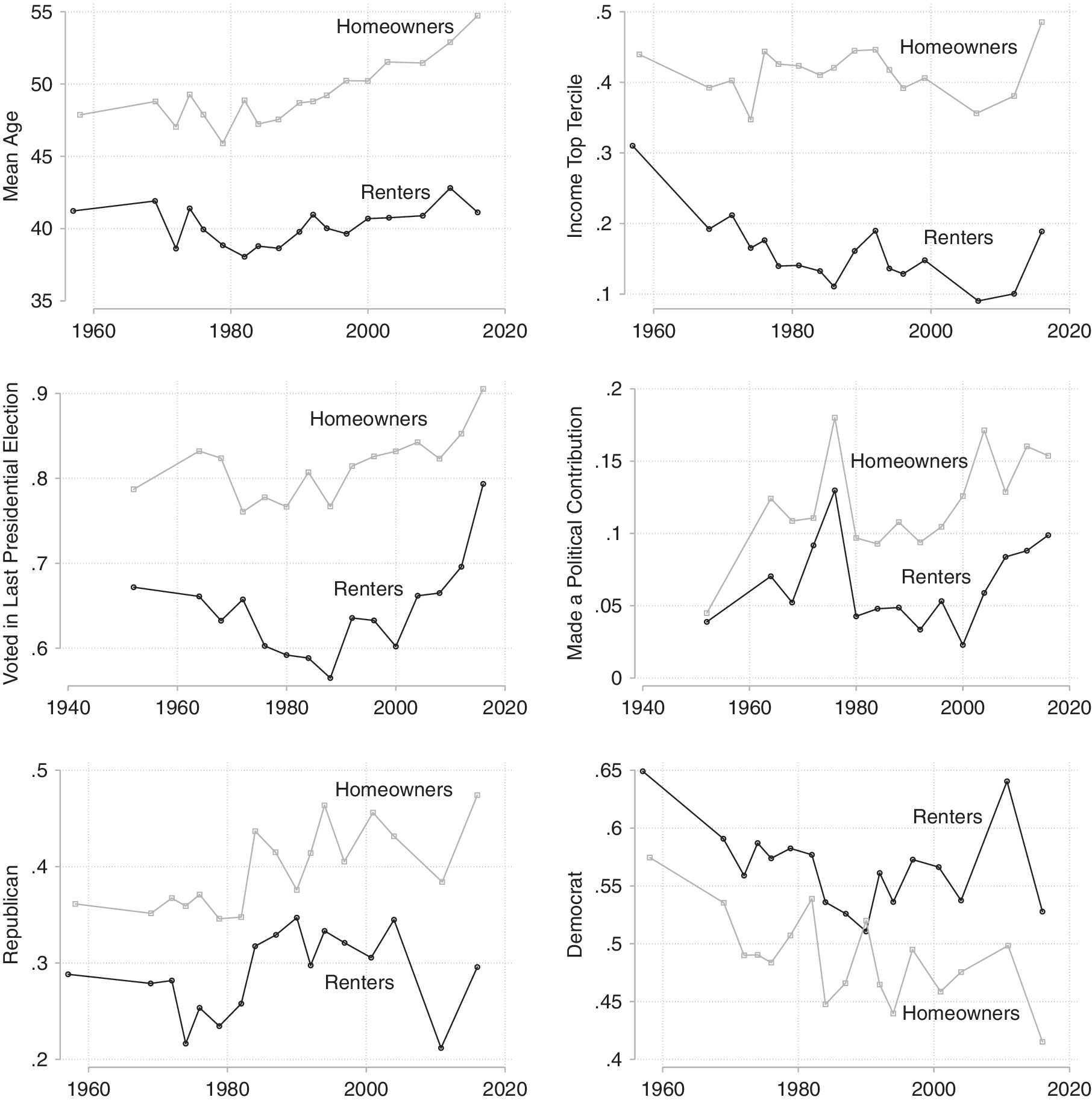
Figure 1 Descriptive Differences between Homeowners and Renters in the United States, ANES Cumulative File.
To move beyond descriptive differences and test the causal link between property ownership and political behavior, I combine individual-level administrative data on property records, voting, political contributions, and an original dataset on public statements made by individuals at local city council meetings. The analyses span from 2000 at the earliest to 2018 at the latest and include over 3.5 million unique individuals from California and Texas, which offers enormous variation across place and time. Using a series of difference-in-differences designs, I find that becoming a property owner increases many forms of political activity: individuals become more likely to participate in local city council meetings, vote in local elections, and donate to candidates in state and federal elections. One of the main advantages of this study is that I observe the same individual’s political behavior both before and after they become a homeowner, meaning I can control for fixed, unobservable characteristics of an individual that affect their likelihood of political participation. A series of follow-up analyses suggests that these changes cannot be wholly attributed to changes in wealth or age, two important potential time-varying confounders. I also document massive inequalities in the types of individuals who participate in local political meetings compared with those who do not. Consistent with previous research, I find that participants in local meetings are more likely to be men, regular voters, and older, on average (Einstein, Palmer, and Glick Reference Einstein, Palmer and Glick2019). These differences vary widely across settings, and I show suggestive evidence that these differences are likely a function of homeowners and renters prioritizing different local issues, coupled with differing topic salience across cities.Footnote 10
Studying individual-level comments and donations also provides other advantages over simply examining turnout. Individuals in large electorates are unlikely to cast a pivotal vote regardless of their homeownership status, so increases in turnout as a result of homeownership would likely come from lowering costs of participation (Downs Reference Downs1957; Riker and Ordeshook Reference Riker and Ordeshook1968).Footnote 11 Given that comments in local meetings are an important way constituents provide information to local politicians (Einstein, Glick, and LeBlanc Reference Einstein, Glick and LeBlanc2017), it is likely a more effective and consequential form of political participation than voting (Brady, Verba, and Schlozman Reference Brady, Verba and Schlozman1995) or making a political contribution (Ansolabehere, De Figueiredo, and Snyder Reference Ansolabehere, De Figueiredo and Snyder2003). The text of public comments in local meetings also sheds light on what motivates individuals to participate in local politics. Using these statements, I find that homeowners and renters focus on different local issues, even after controlling for differences in topic frequency across cities and over time. Homeowners prioritize issues related to development, traffic, and historic preservation, while renters prioritize topics like policing and community programming.
Overall, the evidence suggests that becoming a property owner changes how an individual participates in local politics—and that it boosts their involvement in making costly efforts to shape local politics in the real world. Normatively, these findings illustrate an important trade-off. On one hand, it might be desirable that the structure of local politics in the US encourages homeowners—who have an important share of their wealth concentrated in an immobile asset, and therefore have a large financial stake in the local community—to participate. On the other hand, given the baseline level of wealth necessary to become a property owner, the increase in participation among those who become property owners seems to come at the cost of an electorate that is representative of the broader population, and apparently property ownership, at least in part, contributes to participatory inequalities in local politics.
Data on Homeownership and Political Behavior
To study the effect of homeownership on political behavior, I use individual-level administrative data from four sources. The first dataset has information on property ownership, collected from public records in each county in the United States and provided by CoreLogic, a private data vendor. The dataset includes information about individual properties, including property type, full name of the property’s owner(s), full address, sale date, sale price, assessed value, and other information in each year from 2000–2017. I combine this information with political behavior from three other sources: (1) an original dataset on individuals’ public statements in local city council meetings in Dallas, Texas; Houston, Texas; and Palo Alto, California, assembled from publicly available meeting transcripts, (2) administrative voter files from the entire states of California and Texas, provided by voter file vendor L2, and (3) political contributions in state and federal elections from the Database on Ideology, Money in Politics, and Elections (DIME) (Bonica Reference Bonica2014; Reference Bonica2016).
Each of these datasets provides unique advantages, which I summarize in Table 1. The voter file has individual turnout in local elections over a long period of time, from 2000–2017. That said, the disadvantage is that turnout, even in local elections, is one of the least costly observable forms of political participation. Vote choice is also anonymous, so it is difficult to infer how individuals’ political preferences might be changing by only observing the turnout decision.
Table 1 Information Included in Various Data Sources
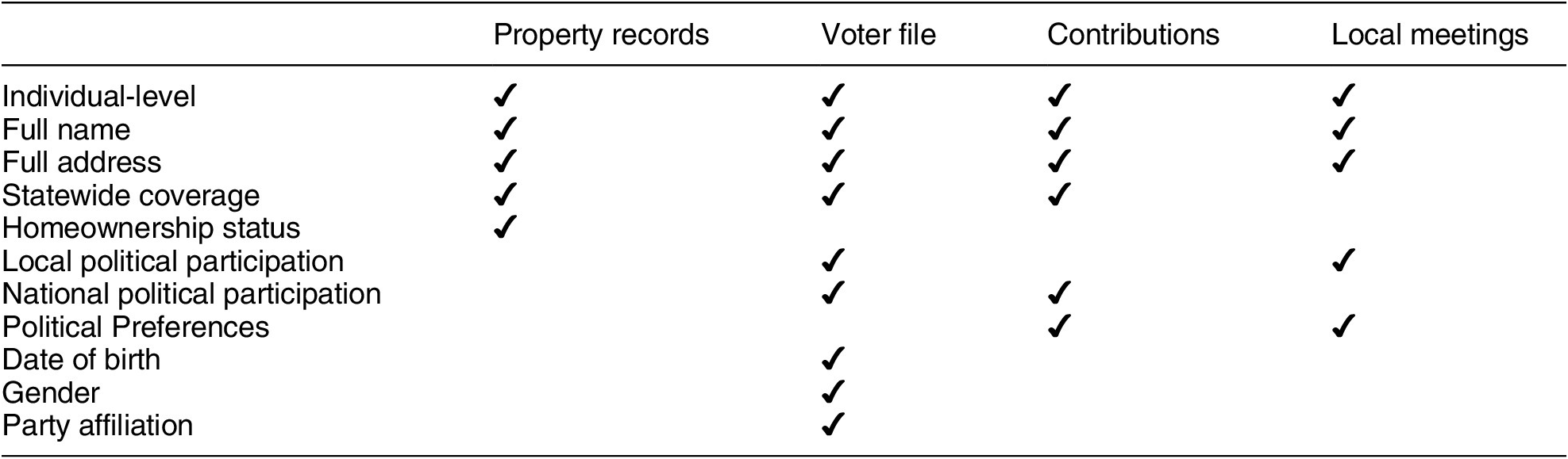
Note: Each column denotes a data source, and check marks indicate features or observable information in that data source.
Local Meetings Data and Case Selection. For a more costly form of participation, I link individuals to political contribution records in state and federal elections from 2000–2014, and I also assemble an original dataset on public statements individuals make at local city council meetings. I collect city council meeting transcripts from Dallas,Footnote 12 Texas (2000–2018), Houston,Footnote 13 Texas (2004–2014), and Palo Alto, California (2002–2010). I chose these cities because of data availability. To be able to merge individual comments to the voter file and property records requires name and address, and most city council meeting transcripts often only include the full name of each individual who comments. Nonetheless, these cases provide some interesting variation in the salience of housing as a local issue. Palo Alto, California has become a focal point for the rise of “not in my backyard” politics, or NIMBYism, where homeowners seek to restrict local housing development to protect their home values, even in cases where these restrictions conflict with partisan ideology (e.g., Marble and Nall Reference Marble and Nall2019). Becoming a homeowner might increase participation at local meetings in settings like Palo Alto, where housing development is a central feature of local political debate, compared with settings like Dallas and Houston. The cities also offer considerable variation in size, population characteristics, and government characteristics.Footnote 14
For each city, I observe the full name and address of each individual who makes a public statement at a city council meeting along with the topic and, in many cases, the full text of their actual spoken statement. In other cases, meeting transcripts provide a summary of the public speaker’s comments. Using these transcripts, I code every instance of a public comment, preserving the name and address of each commenter in order to link them to the voter file, property records, and donation records. The final dataset includes over 7,000 public statements made in local meetings across the three cities.
Linking Individuals across Data Sources
I link individuals using full name and address, which are available in each of the four main data sources: (1) the administrative voter file, (2) property records, (3) individual contribution records, and (4) city council meeting participation. In this section, I describe the procedure for linking individuals across these four sources.
Administrative Voter File
I begin with the full voter file for the states of California and Texas.Footnote 15 For each individual, the file contains full name and address, registration date, date of birth, gender, party affiliation, and turnout history in local and national elections from 2000–2017.
Linking Individuals to Property Records
I link the voter file with property tax and deed records for the entire states of California and Texas. The property records include the full name of each property’s owner(s), address, property type, sale date, sale price, assessed value, and other information. To preprocess the property records, I subset to owners of the following property types: single family residence, condominium, duplex, and apartment. If properties have two owners, I treat each owner as a unique record for the purposes of the merge.Footnote 16 Following recent work in political science on merging individuals across large scale administrative datasets, I implement fastLink (Enamorado, Fifield, and Imai Reference Enamorado, Fifield and Imai2019), a probabilistic record linkage procedure, in order to merge records on first name, last name, zip code, and full street address.Footnote 17 Because each of the datasets contains millions of records, I first block on zip code, and then proceed by matching probabilistically on last name, first name, and full street address.Footnote 18 I set a threshold of 0.85 to declare two records a match, meaning the posterior probability that the two records are a match exceeds 85%. Following Enamorado, Fifield, and Imai (Reference Enamorado, Fifield and Imai2019), I use the match probabilities in the analysis in order to incorporate the merge uncertainty into the post-merge analysis.Footnote 19 After selecting the best match using this procedure, I preserve both unmatched voter file records and unmatched property records for subsequent merges.Footnote 20 This means that individuals in the voter file who do not match to the property records using this procedure are coded as non-homeowners, and homeowners who do not match to the voter file are included and coded as non-voters. I describe the procedure in more detail in Section A.1. Overall, many individuals in the voter file are identified as homeowners: 55.91% of individuals in the voter file are homeowners based on this linkage procedure.Footnote 21
Linking Individuals to Political Contribution Records
Next, I merge in political contribution records for the entire states of California and Texas for each year from 2000 through 2014. These records contain itemized political contributions to candidates or committees for federal and state offices.Footnote 22 Federal races include Presidential, US House, and US Senate races, whereas state races include elections for Governor and state legislature. Because the contributions data contains much of the same information as the voter file and property records, namely zip code, last name, first name, and self-reported address, I use the same probabilistic linkage procedure as the one described for linking the voter file to property records. One limitation of this dataset is that the address is self-reported, meaning a contributor could report a PO Box or a work address, making them more difficult to link to their voter file records or property records. For this reason, the false negative rate is a bit higher (29%) compared with merges using the other datasets. I output the full population of registered voters and property owners, but it now includes information on whether the individual made a contribution in each year from 2000 through 2014, coded as a 0 if I fail to find a contribution record for that individual. For those who made a donation, I observe the amount of all donations, along with the office, party, and ideology of the receiving candidates.Footnote 23 Political donations in a given year are quite rare: about 0.4% of person-years in the dataset make an itemized contribution, overall.Footnote 24
Linking Individuals to City Council Meeting Participation
Finally, I link individuals to an original dataset on public participation in local city council meetings. Each observation in the meetings data is a comment, accompanied by the individual’s full name, address, zip code, and date of the local meeting.Footnote 25 I preprocess the meetings data by collapsing the dataset so that the unit is an individual, and I generate a count of the total number of comments an individual makes in each year. I again rely on the linkage procedure described above. Pooling all three cities together, about 0.27% of residents make a comment at a local city council meeting at some point during the study period. This rate is higher in Palo Alto (1.78%) than in Dallas (0.29%) and Houston (0.21%).
Summary
The final dataset includes over 3.5 million unique individuals in California and Texas, whose vote history is observed since 2000.Footnote 26 This dataset has two main limitations: first, the voter file is only observed at one point, September 2018, so I do not observe individuals who were registered but purged from the voter file before this date. If homeowners are purged from the voter file at different rates than non-homeowners, this would induce bias in the estimated effect of homeownership. Hall and Yoder (Reference Hall and YoderForthcoming) shows that the results for a similar analysis in North Carolina, where voter file histories are available, are very similar when including and excluding purged voters—so this potential source of bias is unlikely to substantially affect the results. The second main limitation is the possibility of merge error. The false positive rate, where a match contains two different individuals who are linked, is often very low when using high-quality administrative datasets containing full name and address (Ansolabehere and Hersh Reference Ansolabehere and Hersh2017; Enamorado, Fifield, and Imai Reference Enamorado, Fifield and Imai2019).Footnote 27 The main concern for this merge would be false negatives, where records in different datasets correspond to the same individual but they are not matched. Because these datasets are high quality, have low missingness, and are unlikely to have widespread misspellings in name and address, the false negative rate should be low compared with most probabilistic linking across administrative datasets. I report the estimated false positive and false negative rates in Section A.1 of the Appendix, and the estimates are reassuringly low, especially when linking the voter file to the property records, where the overall false positive rate is 0.52% and the overall false negative rate is 13.4%.
Characterizing Who Participates in Local Meetings
With the resulting dataset, I characterize the types of individuals who participate in local city council meetings compared with other residents who do not. Figure 2 compares attributes of individuals who spoke at a Palo Alto city council meeting at some point from 2002–2010 with those who did not. Each graph plots the distribution of a given characteristic, and I do this separately for individuals who comment at local city council meetings (in blue) and for those who do not comment at local meetings (in gray). A few interesting patterns emerge. Participants in local city council meetings in Palo Alto are more likely to be registered to vote, older, male, political donors, and voters in local and national elections, on average. The differences in participation in local elections are massive: while non-commenters had a turnout rate of about 24% in local elections during this period, commenters had a turnout rate over 71%. In Palo Alto, local meeting participants are also more likely to be Democrats and are slightly more liberal according to the CF score among donors.Footnote 28 Lastly, commenters are much more likely to be homeowners (62%) than non-commenters (42%).Footnote 29
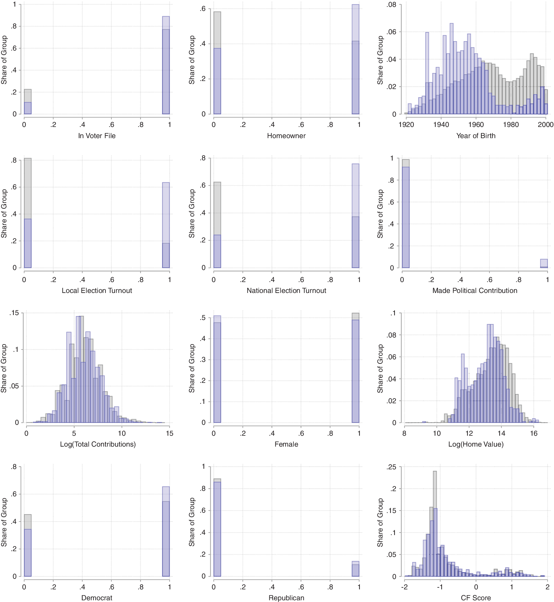
Figure 2 Palo Alto City Council Commenters, 2002–2010
It is possible—and perhaps even expected—that massive differences in the types of people who comment at local meetings and those who do not might not generalize to settings other than Palo Alto for a few reasons. Both the types of individuals who live in Palo Alto and the most salient issues in the city are quite different from those of most other cities. Overall, Palo Alto has higher levels of political participation, both in local and national elections, compared with most areas of the United States. It also has many Democratic registrants: a majority of registrants affiliate with the Democratic party, whereas only about 11% of registrants affiliate with the Republican party. Palo Alto residents have very high education levels—81% have a Bachelor’s degree or higher. Its housing market is also quite out of the ordinary—the median home value exceeds $2 million. And, issues around housing and development are much more salient local issues in Palo Alto than in the vast majority of US cities. All of these quirks raise the question of whether the observed differences between local meeting participants and non-participants generalize to other settings.
To test this, Figure 3 compares attributes of individuals who spoke at a Dallas city council meeting at some point from 2000–2018 with those who did not. Like Palo Alto, commenters in Dallas city council meetings are more likely than non-commenters to be registered to vote, older, male, political donors, and voters in local and national elections, on average. They are also slightly more liberal, looking both at the share that register as Democrats and the CF score among donors. Commenters in Dallas are also more likely to be homeowners (49%) than non-commenters (39%), but this difference is much smaller than the homeownership gap in Palo Alto. This could be because the costs of participation are lower for renters if they live closer to City Hall, or because the salient topics at local meetings motivate homeowners more in Palo Alto than in Dallas. Figure A.2 in the Appendix shows the same set of comparisons for local meeting participants in Houston, and the differences are all quite similar to those in Dallas.
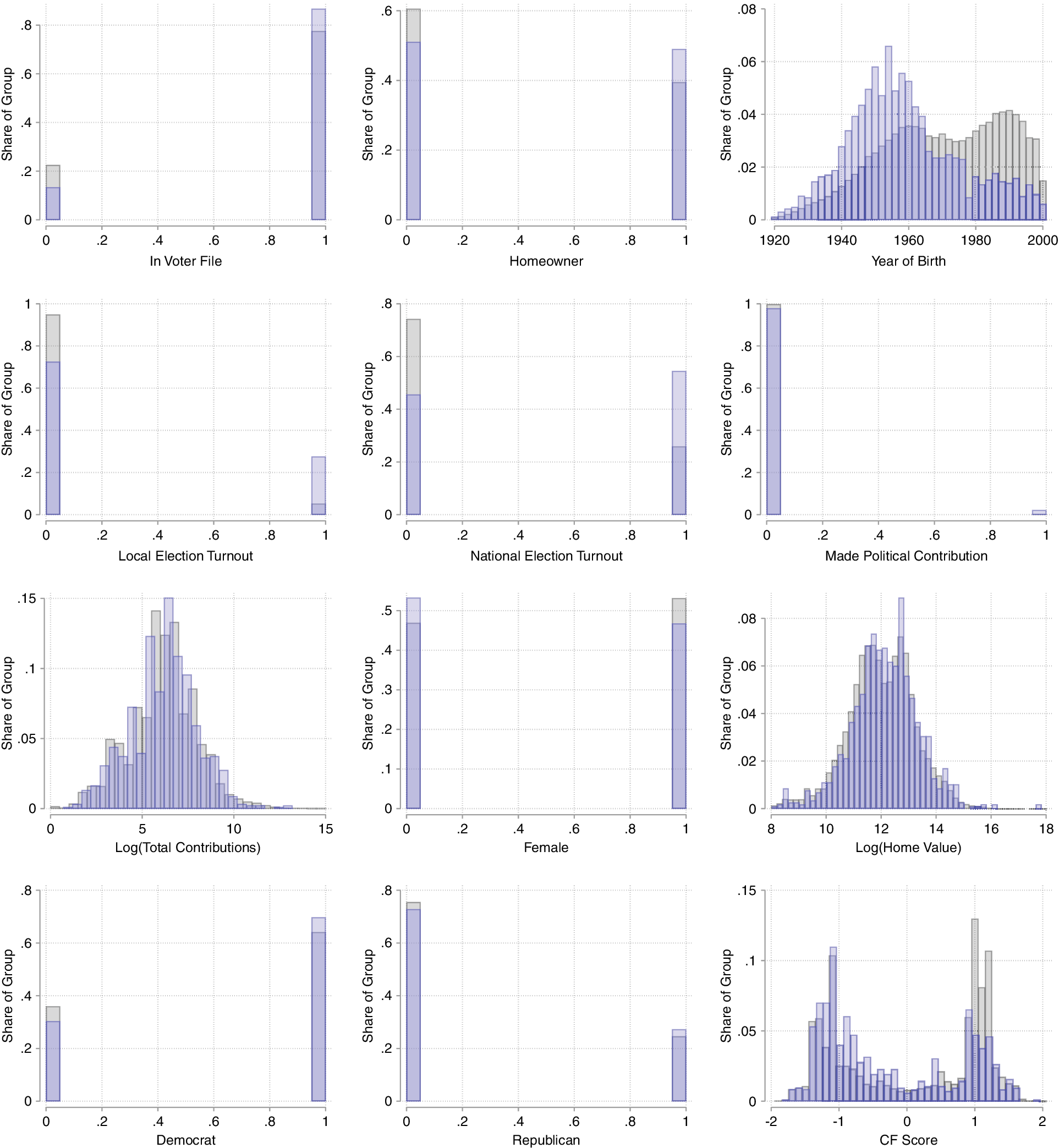
Figure 3 Dallas City Council Commenters, 2000–2018
The first work to systematically document inequalities in participation in local planning and zoning board meetings finds participants in local meetings in Massachusetts are overwhelmingly homeowners (Einstein, Palmer, and Glick Reference Einstein, Palmer and Glick2018). Here, I build on this existing work and show that these inequalities in participation in local meetings extend to other settings, as well as for commenting in city council meetings in addition to meetings specifically about land use.
That said, the share of commenters that are homeowners varies substantially not only across city, but also over time within each city. As Figure 4 shows, the share of commenters in Palo Alto who are homeowners ranges from about 57% (in 2008) to 75% (in 2002). The share of commenters at local meetings in Dallas has increased from around 22% to over 57% from 2000 to 2017. Later, I show that homeowners and renters are motivated by different issues when commenting at local meetings, which could explain this variation within city over time. I show that homeowners are more likely to make comments related to land use policies than are renters, holding city, time, and the meeting agenda fixed, which is consistent with the findings from Einstein, Palmer, and Glick (Reference Einstein, Palmer and Glick2019) that homeowners are much more active in local politics when questions of land use are on the agenda.
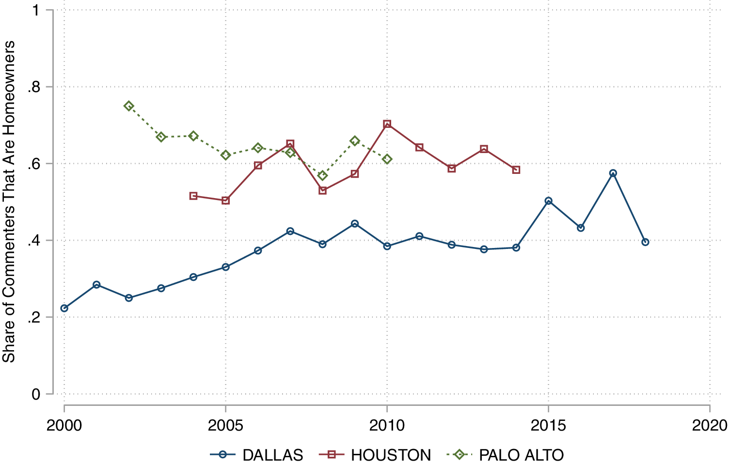
Figure 4 Proportion of Commenters That Are Homeowners over Time, by City
Overall, this section provides systematic evidence documenting inequalities in participation in local city council meetings across different settings. Persistent inequalities in local participation emerge in each of the settings I study (participants are more likely to be older, male, voters, and political donors, on average). The gap in the homeownership rate of commenters and non-commenters, meanwhile, varies widely across different settings: in Palo Alto those who participate in local meetings are over 20 percentage points more likely to be homeowners than those who do not participate, whereas in Dallas and Houston these gaps are substantially smaller. Our understanding of inequalities in political participation at the local level, therefore, requires attention to which types of issues are addressed in local meetings and to what motivates homeowners and renters to participate.
Homeownership Increases Political Participation
So far, I have shown that there are inequalities in local meeting participation across three different cities. Next, to gain some causal leverage on how homeownership changes an individual’s political behavior, I employ a series of difference-in-differences designs to estimate how becoming a property owner affects various forms of political participation. Overall, I find that becoming a homeowner leads to increases in an individual’s likelihood of commenting at local meetings, voting in local elections, and making political contributions.
As discussed in the introduction, for the purposes of these analyses, homeownership, as a conceptual treatment, represents a large monetary investment in an immobile asset situated in a particular geographic location. The counterfactual I have in mind, then, is what an individual homeowner’s political behavior would have looked like had they chosen not to allocate a large fraction of their wealth in becoming a property owner.
Of course, the main threat to this interpretation is that the decision to purchase a home is often correlated with other, often unobservable, changes in an individual’s life—like marriage, changes in income, retirement, or other life events, which in turn might also affect political participation. While I clearly cannot randomize the decision for an individual to purchase a home, I use a series of strategies to test these different mechanisms, including making comparisons only among individuals who are the same age and who have similar levels of wealth, for example. I discuss this more below, but the results suggest that homeownership as an economic investment has a direct effect on an individual’s participation in local politics.
Evidence from Local City Council Meetings
I first estimate the effect of becoming a property owner on an individual’s participation in local city council meetings. Specifically, I estimate the following equation:
 $$ Commente{d}_{it}=\beta Homeowne{r}_{it}+{\gamma}_i+{\delta}_t+{\epsilon}_{it},\kern1.00em \operatorname{} $$
 where  $$ Commente{d}_{it} $$ is an indicator for whether individual
  $$ i $$ comments at a local city council meeting in year
 $$ t $$, and
  $$ Homeowne{r}_{it} $$ is an indicator for whether individual
  $$ i $$ is a property owner at any time in the year prior to the start of year
  $$ t $$. To incorporate the uncertainty in the merge into the estimation, following Enamorado, Fifield, and Imai (Reference Enamorado, Fifield and Imai2019) I multiply the homeowner indicator by the posterior probability of the records being a correct match. The intuition for this is straightforward: this procedure essentially downweights the magnitude of the treatment for individuals where it is less certain that they have been correctly matched.Footnote 30 The individual (
 $$ {\gamma}_i $$) and year (
 $$ {\delta}_t $$) fixed effects control for time-invariant characteristics about individuals that affect their propensity to comment at local meetings as well as common yearly shocks that affect the number of commenters at local city council meetings. Throughout the analyses, I vary the time fixed effects in several ways to estimate effects using different counterfactual trends.
Table 2 estimates the effect of becoming a property owner on participation at local city council meetings. Because participation in city council meetings is a low-probability event, I subset to those who would go on to make a comment at some point over the entire study period, leaving about 6,000 unique individuals, totaling nearly 90,000 observations.Footnote 31 In column 1, I pool all three cities together, and I demonstrate that becoming a homeowner increases an individual’s likelihood of commenting by about 3.9 percentage points, representing about a 50% increase over the outcome mean.Footnote 32 The effect is precisely estimated: the 95% confidence interval ranges from about a 3.1 to 4.7 percentage point increase. I use zip code-by-year fixed effects to compute counterfactual trends using only individuals in the same zip code, but the results also hold across alternative sets of time fixed effects. One concern, however, with the estimates in column 1 is that I use all individuals rather than ones who have lived in the area for the entire study period. For example, if someone were to become a property owner when they newly move into the city, I would count them as not having participated in the local city council meetings before moving there, even though they did not have the opportunity to participate, or they could have been participating in local meetings elsewhere. While I cannot observe the date an individual moved into the city, I can subset to individuals who were registered within the same state since before the start of the study period. This helps alleviate concerns about movers biasing the estimate upward in column 1. In column 2, I estimate the effect just among those who were registered in the state during the entire study period. The estimate increases slightly to about 4.6 percentage points and remains reasonably precisely estimated.
Table 2 Effect of Homeownership on Participation in City Council Meetings, 2000–2018
Note: Robust standard errors clustered by individual in parentheses. The unit of observation is a person-year. Columns 2 through 5 restrict the sample to individuals registered to vote in the state before the panel. All columns restrict the sample to individuals who make a comment at some point over the length of the panel.
In columns 3, 4, and 5, I estimate the effect separately for each city in my data: Palo Alto, Dallas, and Houston, respectively. Becoming a property owner leads an individual to become over 16 percentage points more likely—or nearly twice as likely—to comment at a local city council meeting in Palo Alto, where housing issues are most salient. Becoming a property owner leads individuals to comment more at local meetings in Dallas and Houston as well, but the effects are much more modest in size. While the variation in effect size across cities is insufficient to pin down one particular mechanism, it does suggest that individuals become especially motivated to participate after becoming a property owner in areas where housing issues are more salient, which is consistent with—but of course does not prove—the Fischel (Reference Fischel2001) homevoter hypothesis, where homeowners become more attentive to local politics in places where incentives to protect property values are highest. A later section provides some support for this interpretation, as homeowners tend to focus on issues related to housing policy and development much more than renters, at least in the three cities that I study.
The validity of these difference-in-differences estimates relies on the parallel trends assumption, where changes in individuals’ propensities to comment at local meetings after purchasing a home in a given year would have been the same as changes for those who did not purchase a home in that year. There are reasons to be skeptical of the parallel trends assumption in this particular case. Because homeownership is not randomly assigned, the obvious concern is that any time-varying confounder that correlates both with an individual’s decision to purchase a home and with trends in local meeting participation would bias the estimates. One strategy to assess the difference-in-differences identification strategy is to add a variety of group-specific time trends to allow for different counterfactual trends. Later in the paper, I use this strategy to assess the influence of possible time-varying confounders like wealth, age, planning for children, or other “adult roles” (Highton and Wolfinger Reference Highton and Wolfinger2001). Here, I assess the plausibility of parallel trends in a few other ways. First, in the first two columns of Table A.5 in Appendix I include leads of homeownership, and I do not find strong evidence of pre-trending. Second, in Figures A.4, A.5, and A.6 I include several leads and lags of homeownership, modeling the dynamic effect of homeownership on the probability that an individual comments at local meetings in Palo Alto, Dallas, and Houston, respectively (Angrist and Pischke Reference Angrist and Pischke2008; Autor Reference Autor2003). The estimates show no evidence of an effect in the years before homeownership, with increasing effects in the first few years after becoming a homeowner. This pattern is a reassuring sign that the difference-in-differences identification assumption could hold in this case.
Lastly, I consider an alternative multiperiod difference-in-differences estimator, which allows one to nonparametrically adjust for unit and time unobserved confounders at the same time. The estimator, proposed in Imai and Kim (Reference Imai and Kim2020), is equivalent to a weighted version of the standard two-way fixed effects regression. I show the results using this alternative estimator in Table A.6 in the Appendix, and the results remain similar.
Evidence from Local Turnout
So far, I have shown that property ownership increases an individual’s likelihood of participating in local city council meetings, on average. Now, I turn to its effect on other forms of political participation, starting with turnout in local elections. I rely on difference-in-differences designs to estimate how property ownership changes turnout in local elections in California and Texas from 2001–2017.Footnote 33 The outcome,  $$ Turnou{t}_{it} $$, is a simple indicator for whether individual
  $$ i $$ voted in the general election in time
  $$ t $$. I also use the same procedure for incorporating the merge uncertainty as in the analysis for Table 2.
Wealth is perhaps the most obvious potential time-varying confounder in this setup—where individuals who become wealthier decide to purchase homes and also have different turnout trends for reasons other than the decision to purchase a home. As a first way to address this, I estimate the effect of property ownership on local election turnout only among those who become homeowners at some point—so every individual achieves the wealth status necessary to purchase a home at some point. These estimates, then, exploit variation in the timing of the decision to purchase a home, effectively requiring that changes in turnout among those who purchase a home in time  $$ t $$ would have been the same as changes in turnout among those who did not purchase a home in time
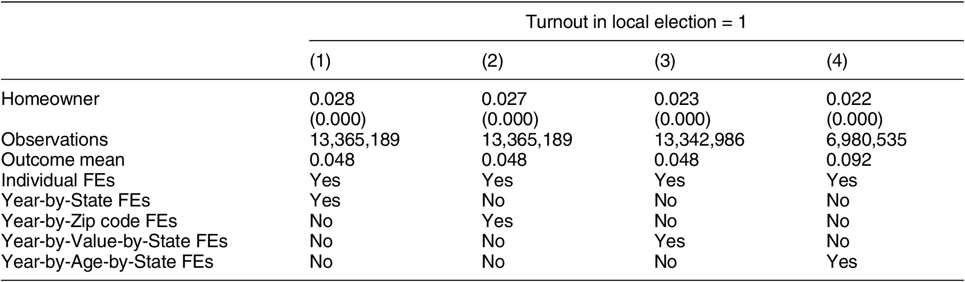
  $$ t $$, but who would later go on to purchase one. This perhaps makes the parallel trends assumption more plausible than including individuals who never become homeowners, who likely have very different counterfactual local turnout trends from individuals who eventually own homes.Footnote 34 In column 1 of Table 3, I include a separate set of year fixed effects for California and Texas, so that counterfactual trends for treated units are constructed only for control units within the same state. In that specification, I find that property ownership leads to a 2.8 percentage point increase in local turnout.Footnote 35 Because changes in local turnout are likely a function of unobserved features like the types of local races or candidates on the ballot, in column 2 I allow each zip code to have its own set of year fixed effects, which constructs counterfactual trends for treated units using only control individuals within the same zip code. The point estimate is similar, which helps alleviate concerns that people are becoming property owners in places where local turnout happens to be increasing anyway because of local factors like the types of races or candidates in these localities.
Table 3 Effect of Homeownership on Political Participation in Local California and Texas Elections, 2001–2017
Note: Robust standard errors clustered by individual in parentheses. All columns include only individuals who become homeowners at some point during the study period. Year-by-Value fixed effects interact years with home value deciles.
Table 4 Effect of Homeownership on Political Contributions, 2000–2014
While I already subset on those who eventually become homeowners to make comparisons among individuals with at least enough wealth to eventually qualify to purchase property, in column 3 I use information on assessed home value to make even more fine-grained comparisons that make wealth less likely to be confounding the result. Following Hall and Yoder (Reference Hall and YoderForthcoming), I include separate year fixed effects for each home value decile in each state, which creates counterfactual trends for those who purchase a home using only individuals who did not purchase a home, but would go on to purchase a similarly priced home in the same state in the future. Again, the point estimate remains similar in magnitude. Lastly, another time-varying confounder could be changes in “adult roles,” like marriage or planning for children.Footnote 36 These factors might encourage long-term residency in a community, which positively correlates with political participation (Gay Reference Gay2012; McCabe Reference McCabe2016). While I cannot measure these directly, I use the individual birth dates to make more plausible counterfactual comparisons. In column 4, I include a set of year fixed effects for every birth year in each state, so that I construct counterfactual trends for those who purchase a home using only control units who share the same birth year and are in the same state.Footnote 37 The point estimate decreases slightly to 0.022, but it still represents more than a 20% increase in local turnout over the baseline mean. This suggests that the effect is likely not explained solely by changes in wealth or taking on other adult roles.
To evaluate the plausibility of the parallel trends assumption, I include leads of property ownership in columns 3 and 4 of Table A.5 in the Appendix. These tests do not reveal evidence of pre-trending, which adds some credibility to the difference-in-differences identification assumption. I also include a lags and leads plot in Figure A.7 of the Appendix, finding that the effects are close to zero before property ownership and grow in local election cycles after becoming a property owner. I discuss these in more detail in Section A.7 of the Appendix, but this is a reassuring sign that parallel trends might hold in this case.
Evidence from Political Contributions
Does homeownership increase costly forms of participation beyond local politics? To answer this question, I estimate how property ownership influences a third form of participation: political contributions to candidates or committees for federal or state elections. These contributions represent a more costly form of participation than voting, but they extend beyond local politics and into an individual’s investment in federal and state elections. The outcome,  $$ Contribute{d}_{it} $$, is an indicator for whether individual
  $$ i $$ made an itemized contribution in year
  $$ t $$.Footnote 38 I restrict the sample to registered voters in the state prior to 2000, the start of the panel.Footnote 39 I do not review each particular estimate, but the motivation for each specification mirrors that in Table 3, which I discuss above.
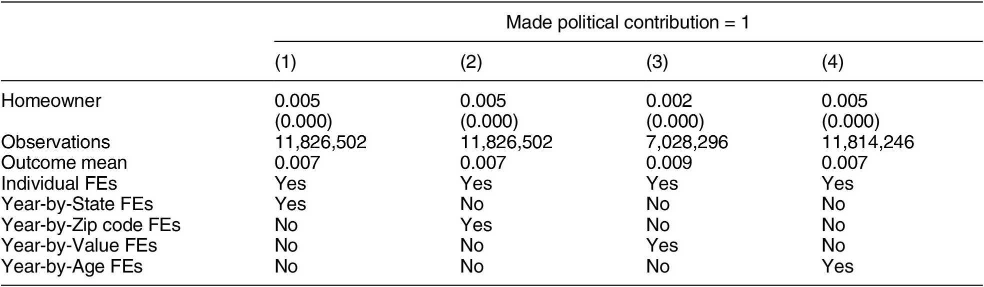
Overall, two notable features stand out. First, across all specifications, homeownership leads to roughly a half percentage point increase in the probability of making a contribution in a given year. Given that the baseline rate of donating is low, this represents nearly a 70% increase. Second, the point estimate in column 3, where I include year-by-home value decile fixed effects, reduces to a 0.2 percentage point increase. Because this specification computes homeowners’ counterfactual trends using only individuals who would eventually go on to buy similarly priced homes but had not yet done so, this suggests we should be concerned that the effects reported in columns 1, 2, and 4 could be biased upward by changes in wealth, an important potential time-varying confounder. This would be plausible because the outcome variable itself requires monetary giving. Wealth and political contributions are positively correlated (Bonica and Rosenthal Reference Bonica and Rosenthal2015), so we might expect this outcome to be especially vulnerable to pre-trending as a function of increased wealth. To check for possible pre-trending, in Figure A.8 in the Appendix I again model the dynamic effect of homeownership, using political contributions as the outcome variable. There is some evidence of pre-trending—the effect of homeownership in year  $$ t $$ on making a contribution in the year
  $$ t-1 $$ is positive and statistically significant, albeit small in magnitude. This is likely because increased wealth correlates both with the decision to purchase a home and the likelihood of making political contribution. Given that, we should prefer the more moderated effect in column 3, which makes comparisons among individuals with more similar levels of wealth. Nonetheless, the evidence suggests that becoming a property owner likely leads to an increase in donating to candidates for federal and state elections, on average.
Homeowners and Renters Focus on Different Issues
So far, I have shown that homeownership increases several forms of participation. But what motivates homeowners and renters to participate in local politics? And why does the gap in participation between homeowners and renters larger in Palo Alto than places like Dallas or Houston? One explanation is simply the parochial nature of small-scale democracy (Oliver, Ha, and Callen Reference Oliver, Ha and Callen2012). Homeowners might be less likely to show up to meetings in Dallas and Houston because those larger cities deal with a wider range of political issues in their local meetings compared with Palo Alto, where questions of land use and development tend to dominate the discussion. Understanding whether homeowners and renters are actually differentiated in the types of topics they raise in local meetings requires a design that holds time, place, and the local meeting agenda fixed.
To do this, I use the text of each comment made by a member of the public at city council meetings in each of the three cities for which I have collected data. Each observation is a comment, which includes the full name, address, and statement that an individual makes in a meeting. Crucially, I also observe the date of the local meeting along with the individual’s homeownership status at the time of the comment, so I can estimate which topics differentiate homeowners from renters within the same local meeting. I implement the linkage procedure described above.
The final dataset includes over 7,000 comments made by individuals at local city council meetings.Footnote 40 To summarize the types of comments, I rely on a structural topic model (STM) to model latent comment topics (Roberts, Stewart, and Tingley Reference Roberts, Stewart and Tingley2014). Similar to latent Dirichlet allocation (LDA) (e.g., Blei, Ng, and Jordan Reference Blei, Ng and Jordan2003), STM is a probabilistic topic model, which assigns each document a vector of weights over distinct topics. Its advantage for my particular context is that STM allows for the inclusion of comment-level covariate information, both to model the prevalence of topics as a function of observable characteristics and to conduct hypothesis testing about the relationships between document characteristics (like the homeownership status of a commenter) and topics that the model discovers (Roberts, Stewart, and Tingley Reference Roberts, Stewart and Tingley2014).
Figure 5 summarizes the top words in each of 10 topics discovered by the model, along with each topic’s frequency.Footnote 41 Because the frequency of topics likely varies both across cities and over time, I include indicators for each city-year in the model to allow time and place to affect the frequency with which a topic is discussed (Roberts, Stewart, and Tingley Reference Roberts, Stewart and Tingley2014). Some of the topics are more interpretable than others: the most frequent topic appears mainly procedural, where the most commonly used words include present, time, call, speak, and name. Other categories have more notable interpretations. Topic 1 appears related to housing and development, as it often uses words like home, house, property, and build. Topic 2 seems related to community programming and policing, commonly using words like community, program, police, and department. Topic 8 seems to be about traffic, using words like parking, street, neighborhood, and traffic.
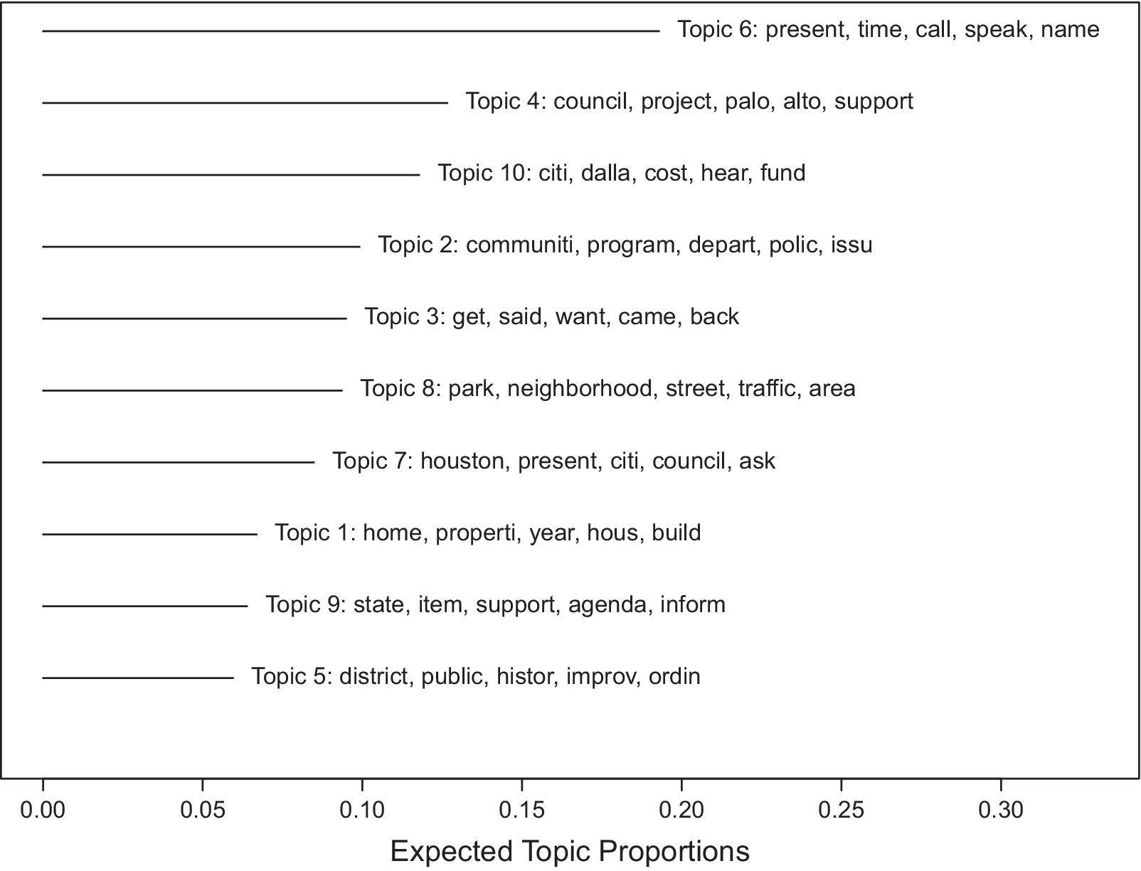
Figure 5 Topic Frequency in Public Statements at City Council Meetings
In Figure 6, I estimate how being a homeowner, as opposed to a renter, changes the proportion of the individual’s comment we would expect to belong to each topic. For each topic, I regress the proportion of the document that falls in the topic on an indicator for whether the commenter is a homeowner, along with city-year fixed effects, which control for unobservable factors that influence the frequency of topics in a city in a particular year. Consistent with expectations about the influence of homeowners in local politics (e.g., Einstein, Palmer, and Glick Reference Einstein, Palmer and Glick2019; Fischel Reference Fischel2001), I find that homeowners’ comments are more likely to belong to topics that reference traffic, housing, property, and development. Meanwhile, renters are relatively more likely to comment on topics related to policing. While this evidence in purely descriptive, it is consistent with the theory that homeowners are motivated to participate in local politics by different issues than are renters. Namely, homeowners are more likely to show up to comment about issues we might expect to relate to preserving their property values—that is, housing and development. Homeowners’ disproportionate appeals to traffic and history are also consistent with qualitative accounts that show homeowners often raise concerns over traffic congestion, historical preservation, and environmental protection as justifications to restrict development (Gerber and Phillips Reference Gerber and Phillips2003; Glaeser and Ward Reference Glaeser and Ward2009).
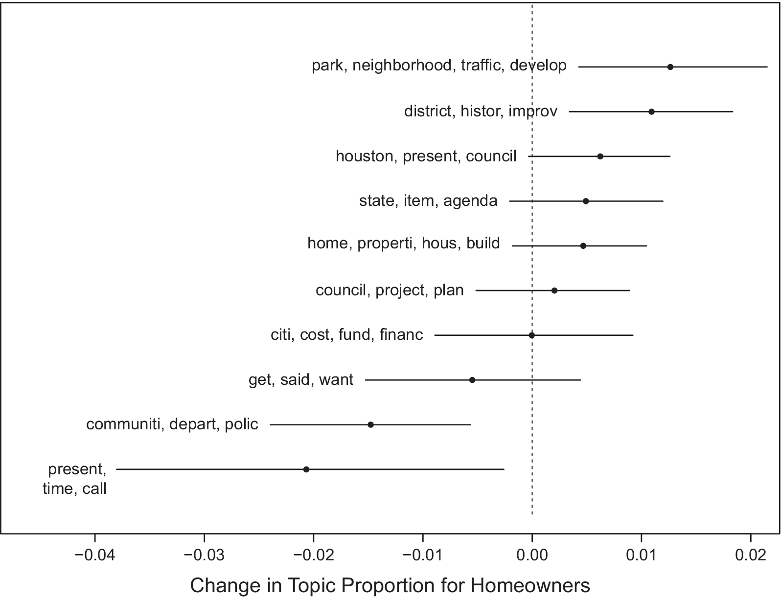
Figure 6 Change in Topic Proportion between Renters and Homeowners
One disadvantage of using STM is that the topics lack a direct interpretation. For a more directly interpretable summary of whether homeowners are more motivated to mention housing development at local meetings than renters, I code each comment according to whether the stems of any of the following words are used in the comment: build, character, development, environment, property, historical, history, home, homeowner, housing, neighborhood, traffic, and zoning. I choose these words because they are generally associated with concerns about housing development and with the reasons offered for supporting or opposing development projects (e.g., Einstein, Palmer, and Glick Reference Einstein, Palmer and Glick2019; Gerber and Phillips Reference Gerber and Phillips2003; Glaeser and Ward Reference Glaeser and Ward2009). Column 1 of Table 5 shows that homeowners are about 9.6 percentage points more likely to use at least one of these housing-related words in their comments compared with renters. To control for changes in the meeting agendas across cities and over time, columns 2 and 3 use city-year fixed effects and meeting fixed effects, which make comparisons between homeowners and renters within the same meeting year and at the same meeting, respectively. In column 3, for example, homeowners are about 7.9 percentage points more likely to use housing-related language than renters, even within the same meeting. This effect is reasonably precisely estimated: the 95% confidence interval spans from a 5.1 to 10.7 percentage point (or 17% to 35%) increase in the likelihood of using housing-related language. Because these differences could be driven by the length of public comments, in columns 4–6 I also estimate the same regressions using a different outcome: the proportion of words in the comment that are any of the housing-related words mentioned above. These results again show that homeowners use language related to housing development more than renters, even when controlling for the city-year, the meeting agenda, and when normalizing by the length of comments.
Table 5 Determinants of Using Housing-Related Language in Public Comments, 2000–2018
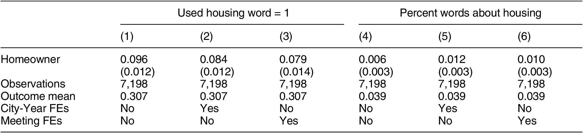
Note: Robust standard errors clustered by meeting in parentheses. The unit of observation is a comment. The outcome in columns 1–3 is whether the commenter used stems of any of the following words in their statement: build, character, development, environment, property, historical, history, home, homeowner, housing, neighborhood, traffic, or zoning. The outcome in columns 4–6 is the share of words in each comment that were stems of these words.
While there are not enough repeat commenters who change homeownership status over the course of the panel to precisely estimate how becoming a homeowner changes the substance of an individual’s comment, this section nonetheless shows that, descriptively, homeowners and renters focus on different issues in local meetings—even within the same meeting where the topics on the agenda are held fixed.
Conclusion
Although there are well-established descriptive relationships between homeownership and political behavior, there is much less work on how the experience of becoming a homeowner changes individual political behavior. In this paper, I contribute to our understanding of how homeownership shapes behavior in three ways. First, using individual comments made by members of the public at local city council meetings, I document large inequalities in who participates in local politics. Individuals who show up and make statements at local meetings are overwhelmingly older, more likely to be male, and much more likely to participate in politics in other ways, like voting in local and national elections as well as making political contributions. Homeowners are drastically over-represented at local meetings in places where housing issues are particularly salient, like Palo Alto. Inequality in local political participation, therefore, is likely a function of the issues that are most salient in the local politics.
Second, I present causal evidence that becoming a homeowner leads individuals to participate more in politics using three separate measures of participation: local meeting comments, voting in local elections, and making political contributions. While the mechanism for these increases is more difficult to pin down, the variation in the effects across geography again points to varying issue salience across different communities. Follow-up analyses suggest that these effects likely cannot be wholly explained by wealth or changing adult roles. The economic incentives associated with property ownership appear to be an important motivator of political participation.
Lastly, I show that homeowners and renters seem to care about different topics in local political meetings, even within the same meeting where the agenda of topics are held fixed. Homeowners are more likely to raise topics related to housing development, consistent with the homevoter hypothesis, where homeowners become motivated to participate in local politics to protect their property value (Fischel Reference Fischel2001).
More broadly, housing policy has increasingly become a central focus of both local and national political discussion, which raises important and fundamental questions about how property ownership motivates and changes political behavior.Footnote 42 With the proliferation of publicly available city council meeting minutes, along with more easily available administrative data at the individual level, researchers have new and exciting opportunities to advance our understanding of exactly how individuals map economic incentives onto their political behavior, both at the local and national level. This paper seeks to understand the political effects of these incentives for one of the most important financial changes in an individual’s lifetime—becoming a property owner. Future work could link voters and property records to other types of administrative data—for example, marriage records—to understand the role of other important influences on political behavior. Discussions in local city council meetings transcripts also present exciting opportunities to further document and understand which local issues are most salient across both place and time and how homeownership or other individual characteristics motivate participation in local politics.
Supplementary Materials
To view supplementary material for this article, please visit http://dx.doi.org/10.1017/S0003055420000556.
Replication materials can be found on Dataverse at: https://doi.org/10.7910/DVN/RDIJQC.


Comments
No Comments have been published for this article.