


Introduction
The standard linear regression is the field’s most commonly encountered quantitative tool, used to estimate effect sizes, adjust for background covariates, and conduct inference. At the same time, the method requires a set of assumptions that have long been acknowledged as problematic (e.g., Achen Reference Achen2002; Leamer Reference Leamer1983; Lenz and Sahn Reference Lenz and Sahn2021; Sami Reference Samii2016). The fear that quantitative inference will reflect these assumptions rather than the design of the study and the data has led our field to explore alternatives including estimation via machine learning (e.g., Beck and Jackman Reference Beck and Jackman1998; Beck, King, and Zheng Reference Beck, King and Zeng2000; Grimmer, Messing, and Westwood Reference Grimmer, Messing and Westwood2017; Hill and Jones Reference Hill and Jones2014) and identification using the analytic tools of causal inference (e.g., Acharya, Backwell, and Sen Reference Acharya, Blackwell and Sen2016; Imai et al. Reference Imai, Keele, Tingley and Yamamoto2011).
I integrate these two literatures tightly, formally, and practically, with a method and associated software that can improve the reliability of quantitative inference in political science and the broader social sciences. In doing so, I make two contributions. First, I introduce to political science the concepts and strategies necessary to integrate machine learning with the standard linear regression model (Athey, Tibshirani, and Wager Reference Athey, Tibshirani and Wager2019; Chernozhukov et al. Reference Chernozhukov, Chetverikov, Demirer, Duflo, Hansen, Newey and Robins2018). Second, I extend this class of models to address two forms of bias of concern to political scientists. Specifically, I adjust for a bias induced by unmodeled treatment effect heterogeneity, highlighted by Aronow and Samii (Reference Aronow and Samii2016). In correcting this bias, and under additional assumptions on the data, the proposed method allows for causal effect estimation whether the treatment variable is continuous or binary. I also adjust for biases induced by exogenous interference, which occurs when an observation’s outcome or treatment is affected by the characteristics of other observations (Manski Reference Manski1993).
The goal is to allow for valid inference that does not rely on a researcher-selected control specification. The proposed method, as with several in this literature, uses a machine learning method to adjust for background variables while returning a linear regression coefficient and standard error for the treatment variable of theoretical interest. Following the double machine learning approach of Chernozhukov et al. (Reference Chernozhukov, Chetverikov, Demirer, Duflo, Hansen, Newey and Robins2018), my method implements a split-sample strategy. This consists of, first, using a machine learning method on one part of the data to construct a control vector that can adjust for nonlinearities and heterogeneities in the background covariates as well as the two biases described above. Then, on the remainder of the data, this control vector is included in a linear regression of the outcome on the treatment. The split-sample strategy serves as a crucial guard against overfitting. By alternating which subsample is used for constructing control variables from the background covariates and which subsample is used for inference and then aggregating the separate estimates, the efficiency lost by splitting the sample can be regained. I illustrate this on experimental data, showing that the proposed method generates point estimates and standard errors no different than those from a full-sample linear regression model.
My primary audience is the applied researcher currently using a linear regression for inference but who may be unsettled by the underlying assumptions. I develop the method first as a tool for descriptive inference, generating a slope coefficient and a standard error on a variable of theoretical interest but relying on machine learning to adjust for background covariates. I then discuss the assumptions necessary to interpret the coefficient as a causal estimate. In order to encourage adoption of the proposed method, software for implementing the proposed method and the diagnostics described in this manuscript are available on the Comprehensive R Archive Network in the package PLCE.
Implications and Applications of the Proposed Method
Quantitative inference in an observational setting requires a properly specified model, meaning the control variables must be observed and entered correctly by the researcher in order to recover an unbiased estimate of the effect of interest. A correct specification, of course, is never known, raising concerns over “model-dependent” inference (King and Zeng Reference King and Zeng2006).
Contrary advice on how to specify controls in a linear regression remains unresolved. This advice ranges from including all the relevant covariates but none of the irrelevant ones (King, Keohane, and Verba Reference King, Keohane and Verba1994, secs. 5.2–5.3), which states rather than resolves the issue; including at most three variables (Achen Reference Achen2002); or at least not all of them (Achen Reference Achen2005); or maybe none of them (Lenz and Sahn Reference Lenz and Sahn2021). Others have advocated for adopting machine learning methods including neural nets (Beck, King, and Zeng Reference Beck, King and Zeng2000), smoothing splines (Beck and Jackman Reference Beck and Jackman1998), nonparametric regression (Hainmueller and Hazlett Reference Hainmueller and Hazlett2013), tree-based methods (Hill and Jones Reference Hill and Jones2014; Montgomery and Olivella Reference Montgomery and Olivella2018), or an average of methods (Grimmer, Messing, and Westwood Reference Grimmer, Messing and Westwood2017).
None of this advice has found wide use. The advice on the linear regression is largely untenable, given that researhers normally have a reasonable idea of which background covariates to include but cannot guarantee that an additive, linear control specification is correct. Machine learning methods offer several important uses, including prediction (Hill and Jones Reference Hill and Jones2014) and uncovering nonlinearities and heterogeneities (Beck, King, and Zeng Reference Beck, King and Zeng2000; Imai and Ratkovic Reference Imai and Ratkovic2013). Estimating these sorts of conditional effects and complex models are useful in problems that involve prediction or discovery. For problems of inference, where the researcher desires a confidence interval or $ p $
-value on a regression coefficient, these methods will generally lead to invalid inference, a point I develop below and illustrate through a simulation study.
$ p $
-value on a regression coefficient, these methods will generally lead to invalid inference, a point I develop below and illustrate through a simulation study.
Providing a reliable and flexible means of controlling for background covariates and clarifying when and whether the estimated effect admits a causal interpretation is essential to the accumulation of knowledge in our field. I provide such a strategy here.
Turning Toward Machine Learning
Conducting valid inference with a linear regression coefficient without specifying how the control variables enter the model has long been studied in the fields of econometrics and statistics (see, e.g., Bickel et al. Reference Bickel, Chris, Ritov and Wellner1998; Newey Reference Newey1994; Robinson Reference Robinson1988; van der Vaart Reference van der Vaart1998, esp. chap. 25). Recent methods have brought these theoretical results to widespread attention by combining machine learning methods to adjust for background covariates with a linear regression for the variable of interest, particularly the double machine learning approach of Chernozhukov et al. (Reference Chernozhukov, Chetverikov, Demirer, Duflo, Hansen, Newey and Robins2018) and the generalized random forest of Athey, Tibshirani, and Wager (Reference Athey, Tibshirani and Wager2019). I work in this same area, introducing the main concepts to political science.
Although well-developed in cognate fields, political methodologists have put forth several additional critiques of linear regression left unaddressed by these aforementioned works. The first critique comes from King (Reference King1990) in the then-nascent subfield of political methodology. In a piece both historical and forward-looking, he argued that unmodeled geographic interference was a first-order concern of the field. More generally, political interactions are often such that interference and interaction across observations is the norm. Most quantitative analyses simply ignore interference. Existing methods that do address it rely on strong modeling assumptions requiring, for example, that interference is being driven by known covariates, like ideology (Hall and Thompson Reference Hall and Thompson2018), or that observations only affect similar or nearby observations either geographically or over a known network (Aronow and Samii Reference Aronow and Samii2017; Ripley Reference Ripley1988; Sobel Reference Sobel2006; Ward and O’Loughlin Reference Ward and O’Loughlin2002), and these models only allow for moderation by covariates specified by the researcher. I extend on these approaches, offering the first method that learns and adjusts for general patterns of exogenous interference.
The second critique emphasizes the limits on using a regression for causal inference in observational studies (see, e.g., Angrist and Pischke, Reference Angrist and Pischke2010, sec 3.3.1). From this approach, I adopt three concerns. The first is a careful attention to modeling the treatment variable. The second is precision in defining the parameter of interest as an aggregate of observation-level effects. Aronow and Samii (Reference Aronow and Samii2016) show that a correlation between treatment effect heterogeneity and variance in the treatment assignment will cause the linear regression coefficient to be biased in estimating the causal effect—even if the background covariates are included properly. I offer the first method that explicitly adjusts for this bias. Third, I provide below a set of assumptions that will allow for a causal interpretation of the estimate returned by the proposed method.
Practical Considerations of the Proposed Method
The major critique of the linear regression, that its assumptions are untenable, is hardly new. Despite this critique, the linear regression has several positive attributes worthy of preservation. First is its transparency and ease of use. The method, its diagnostics, assumptions, and theoretical properties are well-understood and implemented in commonly available software, and they allow for easy inference. Coefficients and standard errors can be used to generate confidence intervals and $ p $
-values, and a statistically significant result provides a necessary piece of evidence that a hypothesized association is present in the data. Importantly, the proposed method maintains these advantages.
$ p $
-values, and a statistically significant result provides a necessary piece of evidence that a hypothesized association is present in the data. Importantly, the proposed method maintains these advantages.
I illustrate these points in a simulation study designed to highlight blind spots of existing methods. I then reanalyze experimental data from Mattes and Weeks (Reference Mattes and Jessica2019), showing that if the linear regression model is in fact correct, my method neither uncovers spurious relationships in the data nor comes at the cost of inflated standard errors. In the second application, I illustrate how to use the method with a continuous treatment. Enos (Reference Enos2016) was forced to dichotomize a continuous treatment, distance from public housing projects, in order to estimate the causal effect of racial threat. To show his results were not model-dependent, he presented results from dichotomizing the variable at 10 different distances. The proposed method handles this situation more naturally, allowing a single estimate of the effect of distance from housing projects on voter turnout.
Anatomy of a Linear Regression
My central focus is in improving estimation and inference on the marginal effect, which is the average effect of a one unit move in a variable of theoretical interest $ {t}_i $
on the predicted value of an outcome
$ {t}_i $
on the predicted value of an outcome $ {y}_i $
, after adjusting for background covariates
$ {y}_i $
, after adjusting for background covariates $ {\mathbf{x}}_i $
.Footnote
1 I will denote the marginal effect as
$ {\mathbf{x}}_i $
.Footnote
1 I will denote the marginal effect as $ \theta $
.
$ \theta $
.
Estimation of the marginal effect is generally done with a linear regression,
 $$ {y}_i\hskip0.35em =\hskip0.35em \theta {t}_i+{\mathbf{x}}_i^T\gamma +{e}_i;\hskip0.66em \unicode{x1D53C}\left({e}_i|{\mathbf{x}}_i,{t}_i\right)\hskip0.35em =\hskip0.35em 0, $$
where the marginal effect $ \theta $
is the target parameter, meaning the parameter on which the researcher wishes to conduct inference.
$ \theta $
is the target parameter, meaning the parameter on which the researcher wishes to conduct inference.
I will refer to terms constructed from the background covariates $ {\mathbf{x}}_i $
and entered into the linear regression as control variables. For example, when including a square term of the third variable
$ {\mathbf{x}}_i $
and entered into the linear regression as control variables. For example, when including a square term of the third variable $ {x}_{3i} $
in the linear regression, the background covariate vector is
$ {x}_{3i} $
in the linear regression, the background covariate vector is $ {\mathbf{x}}_i $
but the control vector is now
$ {\mathbf{x}}_i $
but the control vector is now $ {\left[{\mathbf{x}}_i^T,{x}_{3i}^2\right]}^T $
. I will reserve
$ {\left[{\mathbf{x}}_i^T,{x}_{3i}^2\right]}^T $
. I will reserve $ \gamma $
for slope parameters on control vectors.
$ \gamma $
for slope parameters on control vectors.
Inference on a parameter is valid if its point estimate and standard error can be used to construct confidence intervals and $ p $
-values with the expected theoretical properties. Formally,
$ p $
-values with the expected theoretical properties. Formally, $ \hat{\theta} $
and its estimated standard deviation
$ \hat{\theta} $
and its estimated standard deviation $ {\hat{\sigma}}_{\hat{\theta}} $
allow for valid inference if, for any
$ {\hat{\sigma}}_{\hat{\theta}} $
allow for valid inference if, for any $ \theta $
,
$ \theta $
,
 $$ \sqrt{n}\left(\frac{\hat{\theta}-\theta }{{\hat{\sigma}}_{\hat{\theta}}}\right)\rightsquigarrow \mathbb{N}\left(0,1\right). $$
The limiting distribution of a statistic is the distribution to which its sampling distribution converges (see Wooldridge Reference Wooldridge2013, app. C12), so in the previous display the limiting distribution of the $ z $
-statistic on the left is a standard normal distribution.
$ z $
-statistic on the left is a standard normal distribution.
The remaining elements of the model, the control specification ( $ {\mathbf{x}}_i^T\gamma $
) and the distribution of the error term, are the nuisance components, meaning they are not of direct interest but need to be properly adjusted for in order to allow valid inference on
$ {\mathbf{x}}_i^T\gamma $
) and the distribution of the error term, are the nuisance components, meaning they are not of direct interest but need to be properly adjusted for in order to allow valid inference on $ \theta $
. The component with the control variables is specified in that its precise functional form is assumed by the researcher.
$ \theta $
. The component with the control variables is specified in that its precise functional form is assumed by the researcher.
Heteroskedasticity-consistent (colloquially, “robust”) standard errors allow valid inference on $ \theta $
without requiring the error distribution to be normal, or even equivariant.Footnote
2 In this sense, the error distribution is unspecified. This insight proves critical to the proposed method: valid inference in a statistical model is possible even when components of the model are unspecified.Footnote
3
$ \theta $
without requiring the error distribution to be normal, or even equivariant.Footnote
2 In this sense, the error distribution is unspecified. This insight proves critical to the proposed method: valid inference in a statistical model is possible even when components of the model are unspecified.Footnote
3
In statistical parlance, the linear regression model fit with heteroskedasticity-consistent standard errors is an example of a semiparametric model, as it combines both a specified component ( $ \theta {t}_i+{\boldsymbol{x}}_i^T\gamma $
) and an unspecified component, the error distribution.
$ \theta {t}_i+{\boldsymbol{x}}_i^T\gamma $
) and an unspecified component, the error distribution.
This chain of reasoning then begs the question, can even less be specified? And, does the estimated coefficient admit a causal interpretation? I turn to the first question next and then address the second in the subsequent section.
Moving Beyond Linear Regression
In moving beyond linear regression, I use a machine learning method to construct a control vector that can be included in a linear regression of the outcome on the treatment. This vector will allow for valid inference on $ \theta $
even in the presence of unspecified nonlinearities and interactions in the background covariates. This section relies on the development of double machine learning in Chernozhukov et al. (Reference Chernozhukov, Chetverikov, Demirer, Duflo, Hansen, Newey and Robins2018) and the textbook treatment of van der Vaart (Reference van der Vaart1998). The presentation remains largely informal, with technical details available in Appendix A of the Supplementary Materials. I then extend this approach in the next section.
$ \theta $
even in the presence of unspecified nonlinearities and interactions in the background covariates. This section relies on the development of double machine learning in Chernozhukov et al. (Reference Chernozhukov, Chetverikov, Demirer, Duflo, Hansen, Newey and Robins2018) and the textbook treatment of van der Vaart (Reference van der Vaart1998). The presentation remains largely informal, with technical details available in Appendix A of the Supplementary Materials. I then extend this approach in the next section.
The Partially Linear Model
Rather than entering the background covariates in an additive, linear fashion, they could enter through unspecified functions, $ f,\hskip0.15em g $
:Footnote
4
$ f,\hskip0.15em g $
:Footnote
4
 $$ {y}_i\hskip0.35em =\hskip0.35em \theta {t}_i+f\left({\boldsymbol{x}}_i\right)+{e}_i;\hskip0.33em \unicode{x1D53C}\left({e}_i|{t}_i,{\boldsymbol{x}}_i\right)\hskip0.35em =\hskip0.35em 0. $$
 $$ {t}_i\hskip0.35em =\hskip0.35em g\left({\boldsymbol{x}}_i\right)+{v}_i;\hskip0.66em \unicode{x1D53C}\left({v}_i|{t}_i,{\boldsymbol{x}}_i\right)\hskip0.35em =\hskip0.35em \unicode{x1D53C}\left({e}_i{v}_i|{\boldsymbol{x}}_i\right)\hskip0.35em =\hskip0.35em 0. $$
The resulting model is termed the partially linear model, as it is still linear in the treatment variable but the researcher need not assume a particular control specification. This model subsumes the additive, linear specification, but the functions $ f,\hskip0.15em g $
also allow for nonlinearities and interactions in the covariates.
$ f,\hskip0.15em g $
also allow for nonlinearities and interactions in the covariates.
Semiparametric Efficiency
With linear regression, where the researcher assumes a control specification, the least squares estimates are the uniformly minimum variance unbiased estimate (e.g., Wooldridge Reference Wooldridge2013, sec. 2.3). This efficiency result does not immediately apply to the partially linear model, as a particular form for $ f,\hskip0.15em g $
is not assumed in advance but instead learned from the data. We must instead rely on a different conceptualization of efficiency: semiparametric efficiency.
$ f,\hskip0.15em g $
is not assumed in advance but instead learned from the data. We must instead rely on a different conceptualization of efficiency: semiparametric efficiency.
An estimate of $ \theta $
in the partially linear model is semiparametrically efficient if, first, it allows for valid inference on
$ \theta $
in the partially linear model is semiparametrically efficient if, first, it allows for valid inference on $ \theta $
and, second, its variance is asymptotically indistinguishable from an estimator constructed from the true, but unknown, nuisance functions
$ \theta $
and, second, its variance is asymptotically indistinguishable from an estimator constructed from the true, but unknown, nuisance functions $ f,\hskip0.15em g $
. Establishing this property proceeds in two broad steps.Footnote
5 The first step involves constructing an estimate of
$ f,\hskip0.15em g $
. Establishing this property proceeds in two broad steps.Footnote
5 The first step involves constructing an estimate of $ \theta $
assuming the true functions
$ \theta $
assuming the true functions $ f,\hskip0.15em g $
were known. This estimate is infeasible, as it is constructed from unknown functions. The second step then involves providing assumptions and an estimation strategy such that the feasible estimate constructed from the estimated functions
$ f,\hskip0.15em g $
were known. This estimate is infeasible, as it is constructed from unknown functions. The second step then involves providing assumptions and an estimation strategy such that the feasible estimate constructed from the estimated functions $ \hat{f},\hskip0.15em \hat{g} $
shares the same limiting distribution as the infeasible estimate constructed from
$ \hat{f},\hskip0.15em \hat{g} $
shares the same limiting distribution as the infeasible estimate constructed from $ f,\hskip0.15em g $
.
$ f,\hskip0.15em g $
.
For the first step, consider the reduced form model that combines the two models in Equations 3 and 4,
 $$ {y}_i\hskip0.35em =\hskip0.35em \theta {t}_i+\left[f\left({\boldsymbol{x}}_i\right),g\left({\boldsymbol{x}}_i\right)\right]\gamma +{e}_i. $$
If $ f,\hskip0.15em g $
were known,
$ f,\hskip0.15em g $
were known, $ \theta $
could be estimated efficiently using least squares.Footnote
6 The estimate,
$ \theta $
could be estimated efficiently using least squares.Footnote
6 The estimate, $ \hat{\theta} $
will be efficient and allow for valid inference on
$ \hat{\theta} $
will be efficient and allow for valid inference on $ \theta $
.
$ \theta $
.
Following Stein (Reference Stein and Neyman1956), we would not expect any feasible estimator to outperform this infeasible estimator, so its limiting distribution is termed the semiparametric efficiency bound. With this bound established, I now turn to generating a feasible estimate that shares a limiting distribution with this infeasible estimate.
Double Machine Learning for Semiparametrically Efficient Estimation
Estimated functions $ \hat{f},\hskip0.15em \hat{g} $
, presumably estimated using a machine learning method, can be used to construct and enter control variables into a linear regression as
$ \hat{f},\hskip0.15em \hat{g} $
, presumably estimated using a machine learning method, can be used to construct and enter control variables into a linear regression as
 $$ {y}_i\hskip0.35em =\hskip0.35em \theta {t}_i+\left[\hat{f}\left({\mathbf{x}}_i\right),\hat{g}\left({\mathbf{x}}_i\right)\right]\gamma +{e}_i. $$
Semiparametric efficiency can be established by characterizing and eliminating the gap between the infeasible model in Equation 5 and the feasible model in Equation 6. I do so by introducing approximation error terms,
 $$ {\varDelta}_{\hat{f},i}\hskip0.35em =\hskip0.35em \hat{f}\left({\mathbf{x}}_i\right)-f\left({\mathbf{x}}_i\right);\hskip0.33em {\varDelta}_{\hat{g},i}\hskip0.35em =\hskip0.35em \hat{g}\left({\mathbf{x}}_i\right)-g\left({\mathbf{x}}_i\right), $$
that capture the distance between the true functions $ f,\hskip0.15em g $
and their estimates
$ f,\hskip0.15em g $
and their estimates $ \hat{f},\hskip0.15em \hat{g} $
at each
$ \hat{f},\hskip0.15em \hat{g} $
at each $ {\mathbf{x}}_i $
.
$ {\mathbf{x}}_i $
.
Given these approximation errors, Equation 6 can be rewritten in the familiar form of a measurement error problem (Wooldridge Reference Wooldridge2013, chap. 9.4), where the estimated functions $ \hat{f},\hskip0.15em \hat{g} $
can be thought of as “mismeasuring” the true functions
$ \hat{f},\hskip0.15em \hat{g} $
can be thought of as “mismeasuring” the true functions $ f,\hskip0.15em g $
:
$ f,\hskip0.15em g $
:
 $$ {y}_i\hskip0.35em =\hskip0.35em \theta {t}_i+\left[f\left({\mathbf{x}}_i\right),g\left({\mathbf{x}}_i\right)\right]{\gamma}_1+\left[\hat{f}\left({\mathbf{x}}_i\right)-f\left({\mathbf{x}}_i\right),\hat{g}\left({\mathbf{x}}_i\right)-g\left({\mathbf{x}}_i\right)\right]{\gamma}_2+{e}_i. $$
 $$ {y}_i\hskip0.35em =\hskip0.35em \theta {t}_i+\left[f\left({\mathbf{x}}_i\right),g\left({\mathbf{x}}_i\right)\right]{\gamma}_1+\left[{\varDelta}_{\hat{f},i},{\varDelta}_{\hat{g},i}\right]{\gamma}_2+{e}_i. $$
Establishing semiparametric efficiency of a feasible estimator, then, consists of establishing a set of assumptions and an estimation strategy that leaves the approximation error terms asymptotically negligible.
There are two pathways by which the approximation error terms may bias an estimate. The first is if the approximation errors do not tend toward zero. Eliminating this bias requires that the approximation errors vanish asymptotically, specifically at an $ {n}^{1/4} $
rate.Footnote
7 Though seemingly technical, this assumption is actually liberating. Many modern machine learning methods that are used in political science provably achieve this rate (Chernozhukov et al. Reference Chernozhukov, Chetverikov, Demirer, Duflo, Hansen, Newey and Robins2018), including random forests (Hill and Jones Reference Hill and Jones2014; Montgomery and Olivella Reference Montgomery and Olivella2018), neural networks (Beck, King, and Zeng Reference Beck, King and Zeng2000), and sparse regression models (Ratkovic and Tingley Reference Ratkovic and Tingley2017). This assumption allows the researcher to condense all the background covariates into a control vector constructed from
$ {n}^{1/4} $
rate.Footnote
7 Though seemingly technical, this assumption is actually liberating. Many modern machine learning methods that are used in political science provably achieve this rate (Chernozhukov et al. Reference Chernozhukov, Chetverikov, Demirer, Duflo, Hansen, Newey and Robins2018), including random forests (Hill and Jones Reference Hill and Jones2014; Montgomery and Olivella Reference Montgomery and Olivella2018), neural networks (Beck, King, and Zeng Reference Beck, King and Zeng2000), and sparse regression models (Ratkovic and Tingley Reference Ratkovic and Tingley2017). This assumption allows the researcher to condense all the background covariates into a control vector constructed from $ \hat{f},\hat{g} $
, where these functions are estimated via a flexible machine learning method. Any nonlinearities and interactions in the background covariates are then learned from the data rather than specified by the researcher.
$ \hat{f},\hat{g} $
, where these functions are estimated via a flexible machine learning method. Any nonlinearities and interactions in the background covariates are then learned from the data rather than specified by the researcher.
Eliminating the second pathway requires that any correlation between the approximation errors $ {\varDelta}_{\hat{f},i},\hskip0.35em {\varDelta}_{\hat{g},i} $
and the error terms
$ {\varDelta}_{\hat{f},i},\hskip0.35em {\varDelta}_{\hat{g},i} $
and the error terms $ {e}_i,{v}_i $
tend toward zero.Footnote
8 Doing so requires addressing a subtle aspect of the approximation error: the estimates
$ {e}_i,{v}_i $
tend toward zero.Footnote
8 Doing so requires addressing a subtle aspect of the approximation error: the estimates $ \hat{f},\hat{g} $
are themselves functions of
$ \hat{f},\hat{g} $
are themselves functions of $ {e}_i,{v}_i $
, as they are estimates constructed from a single observed sample. Even under the previous assumption on the convergence rate of
$ {e}_i,{v}_i $
, as they are estimates constructed from a single observed sample. Even under the previous assumption on the convergence rate of $ \hat{f},\hat{g} $
, this bias term may persist.
$ \hat{f},\hat{g} $
, this bias term may persist.
The most elegant, and direct, way to eliminate this bias is to employ a split-sample strategy, as shown in Table 1.Footnote
9 First, the data are split in half into subsamples denoted $ {\mathcal{S}}_1 $
and
$ {\mathcal{S}}_1 $
and $ {\mathcal{S}}_2 $
of size
$ {\mathcal{S}}_2 $
of size $ {n}_1 $
and
$ {n}_1 $
and $ {n}_2 $
such that
$ {n}_2 $
such that $ {n}_1+{n}_2\hskip0.35em =\hskip0.35em n. $
Data from
$ {n}_1+{n}_2\hskip0.35em =\hskip0.35em n. $
Data from $ {\mathcal{S}}_1 $
are used to learn
$ {\mathcal{S}}_1 $
are used to learn $ \hat{f},\hat{g} $
and data from
$ \hat{f},\hat{g} $
and data from $ {\mathcal{S}}_2 $
to conduct inference on
$ {\mathcal{S}}_2 $
to conduct inference on $ \theta $
. Because the nuisance functions are learned on data wholly separate from that on which inference is conducted, this bias term tends toward zero. The resultant estimate is semiparametrically efficient, under the conditions given in in 4.3.
$ \theta $
. Because the nuisance functions are learned on data wholly separate from that on which inference is conducted, this bias term tends toward zero. The resultant estimate is semiparametrically efficient, under the conditions given in in 4.3.
Table 1. The Double Machine Learning Algorithm of Chernozhukov et al. (Reference Chernozhukov, Chetverikov, Demirer, Duflo, Hansen, Newey and Robins2018)
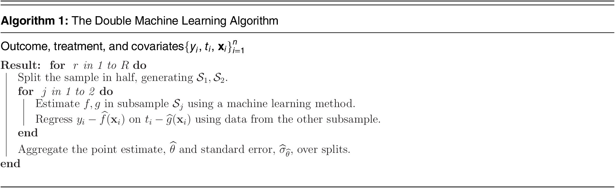
Note:The double machine learning algorithm combines machine learning, to learn how the covariates enter the model, with a regression for the coefficient of interest. Each step is done on a separate subsample of the data (sample-splitting), the roles of the two subsamples are swapped (cross-fitting), and the estimate results from aggregating over multiple cross-fit estimates (repeated cross-fitting). The proposed method builds on these strategies while adjusting for several forms of bias ignored by the double machine learning strategy.
Sample-splitting raises real efficiency concerns, as it uses only half the data for inference and thereby inflates standard errors by $ \sqrt{2}\approx 1.4 $
. In order to restore efficiency, double machine learning implements a cross-fitting strategy, whereby the roles of the subsamples
$ \sqrt{2}\approx 1.4 $
. In order to restore efficiency, double machine learning implements a cross-fitting strategy, whereby the roles of the subsamples $ {\mathcal{S}}_1,{\mathcal{S}}_2 $
are swapped and the estimates combined. Repeated cross-fitting consists of aggregating estimates over multiple cross-fits, allowing all the data to be used in estimation and returning results that are not sensitive to how the data is split. A description of the algorithm appears in Table 1.
$ {\mathcal{S}}_1,{\mathcal{S}}_2 $
are swapped and the estimates combined. Repeated cross-fitting consists of aggregating estimates over multiple cross-fits, allowing all the data to be used in estimation and returning results that are not sensitive to how the data is split. A description of the algorithm appears in Table 1.
Constructing Covariates and Second-Order Semiparametric Efficiency
My first advance over the double machine learning strategy of Chernozhukov et al. (Reference Chernozhukov, Chetverikov, Demirer, Duflo, Hansen, Newey and Robins2018) is constructing a set of covariates that will further refine the estimates of the nuisance functions. Doing so gives more assurance that the method will, in fact, adjust for the true nuisance functions $ f,\hskip0.15em g $
.
$ f,\hskip0.15em g $
.
In order to do so, consider the approximation
 $$ \hat{f}\left({\mathbf{x}}_i\right)\approx f\left({\mathbf{x}}_i\right)+{U}_{f,i}^T{\gamma}_f;\hskip0.66em \hat{g}\left({\mathbf{x}}_i\right)\approx g\left({\mathbf{x}}_i\right)+{U}_{g,i}^T{\gamma}_g $$
or, equivalently,
 $$ {\varDelta}_{\hat{f},i}\approx {U}_{f,i}^T{\gamma}_f;\hskip0.66em {\varDelta}_{\hat{g},i}\approx {U}_{g,i}^T{\gamma}_g $$
for some vector of parameters $ {\gamma}_f,{\gamma}_g $
.
$ {\gamma}_f,{\gamma}_g $
.
These new vectors of control variables $ {U}_{f,i},{U}_{g,i} $
capture the fluctuations of the estimated functions
$ {U}_{f,i},{U}_{g,i} $
capture the fluctuations of the estimated functions $ \hat{f},\hat{g} $
around the true values,
$ \hat{f},\hat{g} $
around the true values, $ f,\hskip0.15em g $
. The expected fluctuation of an estimate around its true value is measured by its standard error (Wooldridge Reference Wooldridge2013, sec. 2.5), so I construct these control variables from the variance matrix of the estimates themselves. Denoting as
$ f,\hskip0.15em g $
. The expected fluctuation of an estimate around its true value is measured by its standard error (Wooldridge Reference Wooldridge2013, sec. 2.5), so I construct these control variables from the variance matrix of the estimates themselves. Denoting as $ \hat{f}\left(\mathbf{X}\right),\hskip2pt \hat{g}\left(\mathbf{X}\right) $
the vectors of estimated nuisance component
$ \hat{f}\left(\mathbf{X}\right),\hskip2pt \hat{g}\left(\mathbf{X}\right) $
the vectors of estimated nuisance component $ \hat{f},\hskip2pt \hat{g} $
, I first construct the variance matrices
$ \hat{f},\hskip2pt \hat{g} $
, I first construct the variance matrices $ \widehat{\mathrm{Var}}\left(\hat{f}\left(\mathbf{X}\right)\right) $
and
$ \widehat{\mathrm{Var}}\left(\hat{f}\left(\mathbf{X}\right)\right) $
and $ \widehat{\mathrm{Var}}\left(\hat{g}\left(\mathbf{X}\right)\right) $
. In order to summarize these matrices, I construct the control vectors
$ \widehat{\mathrm{Var}}\left(\hat{g}\left(\mathbf{X}\right)\right) $
. In order to summarize these matrices, I construct the control vectors $ {\hat{U}}_{\hat{f},i},{\hat{U}}_{\hat{g},i} $
from principal components of the square root of the variance matrices.Footnote
10
$ {\hat{U}}_{\hat{f},i},{\hat{U}}_{\hat{g},i} $
from principal components of the square root of the variance matrices.Footnote
10
Including these constructed covariates as control variables offers advantages both practical and theoretical. As a practical matter, augmenting the control set $ \hat{f},\hskip2pt \hat{g} $
with the constructed control vectors
$ \hat{f},\hskip2pt \hat{g} $
with the constructed control vectors $ {\hat{U}}_{\hat{f},i},{\hat{U}}_{\hat{g},i} $
helps guard against misspecification or chance error in the estimates
$ {\hat{U}}_{\hat{f},i},{\hat{U}}_{\hat{g},i} $
helps guard against misspecification or chance error in the estimates $ \hat{f},\hat{g} $
, adding an extra layer of accuracy to the estimate and making it more likely that the method will properly adjust for
$ \hat{f},\hat{g} $
, adding an extra layer of accuracy to the estimate and making it more likely that the method will properly adjust for $ f\operatorname{}\hskip0.15em $
.
$ f\operatorname{}\hskip0.15em $
.
As a theoretical matter, the method is an example of a second-order semiparametrically efficient estimator. Double machine learning is first-order semiparametrically efficient because it only adjusts for the conditional means $ \hskip2pt \hat{f},\hskip2pt \hat{g} $
. By including the estimated controls
$ \hskip2pt \hat{f},\hskip2pt \hat{g} $
. By including the estimated controls $ \hskip2pt \hat{f},\hskip2pt \hat{g} $
but also principal components
$ \hskip2pt \hat{f},\hskip2pt \hat{g} $
but also principal components $ {U}_{\hat{f},i},\hskip2pt {U}_{\hat{g},i} $
constructed from the variance (the second moment, see Wooldridge Reference Wooldridge2013, app. D.7), the estimates gain an extra order of efficiency and return a second-order semiparametrically efficient estimate.Footnote
11 The theoretical gain is that second-order efficiency requires only an
$ {U}_{\hat{f},i},\hskip2pt {U}_{\hat{g},i} $
constructed from the variance (the second moment, see Wooldridge Reference Wooldridge2013, app. D.7), the estimates gain an extra order of efficiency and return a second-order semiparametrically efficient estimate.Footnote
11 The theoretical gain is that second-order efficiency requires only an $ {n}^{1/8} $
order of convergence on the nuisance terms rather than
$ {n}^{1/8} $
order of convergence on the nuisance terms rather than $ {n}^{1/4} $
. Although seemingly technical, this simply means that the method allows valid inference on
$ {n}^{1/4} $
. Although seemingly technical, this simply means that the method allows valid inference on $ \theta $
while demanding less accuracy from the machine learning method estimating the nuisance terms. At the most intuitive level, including these additional control vectors makes it more likely that the nuisance terms will be captured, with the sample-splitting guarding against overfitting.
$ \theta $
while demanding less accuracy from the machine learning method estimating the nuisance terms. At the most intuitive level, including these additional control vectors makes it more likely that the nuisance terms will be captured, with the sample-splitting guarding against overfitting.
Improving on the Partially Linear Model
Double machine learning addresses a particular issue—namely learning how the background covariates enter the model. Several issues of interest to political scientists remain unaddressed. I turn to these next, which comprise my central contributions.
Adjusting for Treatment Effect Heterogeneity Bias
Aronow and Samii (Reference Aronow2016) show that the linear regression estimate of a coefficient on the treatment variable is biased for the marginal effect. The bias emerges through insufficient care in modeling the treatment variable and heterogeneity in the treatment effect, and the authors highlight this bias as a critical difference between a linear regression estimate and a causal estimate.
To see this bias, denote as $ {\theta}_i $
the effect of the treatment on the outcome for observation i such that the marginal effect is defined as
$ {\theta}_i $
the effect of the treatment on the outcome for observation i such that the marginal effect is defined as $ \theta \hskip0.35em =\hskip0.35em \unicode{x1D53C}\left({\theta}_i\right) $
. To simplify matters, presume the true functions
$ \theta \hskip0.35em =\hskip0.35em \unicode{x1D53C}\left({\theta}_i\right) $
. To simplify matters, presume the true functions $ f\operatorname{}\hskip0.15em g $
are known, allowing a regression to isolate as-if random fluctuations of
$ f\operatorname{}\hskip0.15em g $
are known, allowing a regression to isolate as-if random fluctuations of $ {e}_i,\hskip1.5pt {v}_i $
. Incorporating the heterogeneity in
$ {e}_i,\hskip1.5pt {v}_i $
. Incorporating the heterogeneity in $ {\theta}_i $
into the partially linear model gives
$ {\theta}_i $
into the partially linear model gives
 $$ \hskip-3em {y}_i\hskip0.35em =\hskip0.35em {t}_i{\theta}_i+\left[f\left({\mathbf{x}}_i\right),g\left({\mathbf{x}}_i\right)\right]\gamma +{e}_i $$
 $$ \hskip4.3em =\hskip0.35em {t}_i\theta +{t}_i\left({\theta}_i-\theta \right)+\left[f\left({\mathbf{x}}_i\right),g\left({\mathbf{x}}_i\right)\right]\gamma +{e}_i. $$
The unmodeled effect heterogeneity introduces an omitted variable, $ {t}_i\left({\theta}_i-\theta \right) $
, which gives a bias ofFootnote
12
$ {t}_i\left({\theta}_i-\theta \right) $
, which gives a bias ofFootnote
12
 $$ \unicode{x1D53C}\left(\hat{\theta}-\theta \right)\hskip0.35em =\hskip0.35em \frac{\;\unicode{x1D53C}\left\{\mathrm{Cov}\Big({t}_i,{t}_i\left({\theta}_i-\theta \right)|{\mathbf{x}}_i\Big)\right\}}{\unicode{x1D53C}\left\{\mathrm{Var}\left({t}_i|{\mathbf{x}}_i\right)\right\}} $$
 $$ \hskip0.35em =\hskip0.35em \frac{\unicode{x1D53C}\left({v}_i^2\left({\theta}_i-\theta \right)\right)}{\unicode{x1D53C}\left({v}_i^2\right)}, $$
which I will refer to as treatment effect heterogeneity bias.
Inspection reveals that either one of two conditions are sufficient to guarantee that the treatment heterogeneity variance bias is zero. The first occurs when there is no treatment effect heterogeneity ( $ {\theta}_i\hskip0.35em =\hskip0.35em \theta $
for all observations), and the second when there is no treatment assignment heteroskedasticity—
$ {\theta}_i\hskip0.35em =\hskip0.35em \theta $
for all observations), and the second when there is no treatment assignment heteroskedasticity— $ \unicode{x1D53C}\left({v}_i^2\right) $
is constant across observations. As observational studies rarely justify either assumption (see Samii Reference Samii2016, for a more complete discussion), researchers are left with a gap between the marginal effect
$ \unicode{x1D53C}\left({v}_i^2\right) $
is constant across observations. As observational studies rarely justify either assumption (see Samii Reference Samii2016, for a more complete discussion), researchers are left with a gap between the marginal effect $ \theta $
and the parameter estimated by the partially linear model.
$ \theta $
and the parameter estimated by the partially linear model.
I will address this form of bias through modeling the random component in the treatment assignment. As with modeling the conditional means through unspecified nuisance functions, I will introduce an additional function that will capture heteroskedasticity in the treatment variable.
Interference and Group-Level Effects
The proposed method also adjusts for group-level effects and interference. For the first, researchers commonly encounter data with some known grouping, say at the state, province, or country level. To accommodate these studies, I incorporate random effect estimation into the model. The proposed method also adjusts for interference, where observations may be affected by observations that are similar in some respects (“homophily”) or different in some respects (“heterophily”). For example, observations that are geographically proximal may behave similarly (Ripley Reference Ripley1988; Ward and O’Loughlin Reference Ward and O’Loughlin2002), actors may be connected via a social network (Aronow and Samii Reference Aronow and Samii2017; Sobel Reference Sobel2006), or social actors may react to ideologues on the other end of the political divide (Hall and Thompson Reference Hall and Thompson2018). In each setting, some part of an observation’s outcome may be attributable to the characteristics of other observations.
Existing approaches require a priori knowledge over what variables drive the interference as well as how the interference affects both the treatment variable and the outcome. Instead, I use a machine learning method to learn the type of interference in the data: what variables are driving interference and in what manner.
The problem involves two components: a measure of proximity and an interferent. The proximity measure addresses which variables are driving how close two observations are.Footnote 13 In the spatial setting, for example, these may be latitude and longitude. Alternatively, observations closer in age may behave similarly (homophily) or observations with different education levels may behave similarly (heterophily). The strength of the interference is governed by a bandwidth parameter, which characterizes the radius of influence of proximal observations on a given observation. For example, with a larger bandwidth, interference may be measurable between people within a ten-year age range, but for a narrower bandwidth, it may only be discernible within a three-year range. The interferent is the variable that affects other observations. For example, the treatment level of a given observation may be driven in part by the income level (the interferent) of other observations with a similar age (the proximity measure).
The method learns and adjusts for two types of interference: that driven entirely by covariates and the effect of one observations’ treatment on other observations’ outcomes. For example, if the interference among observations is driven entirely by exogenous covariates, such as age or geography, the method allows for valid inference on $ \theta $
. Similarly, if there are spillovers such that one observation’s treatment affects another’s outcome, as with, say, vaccination, the method can adjust for this form of spillover (e.g., Hudgens and Halloran Reference Hudgens and Halloran2008).Footnote
14
$ \theta $
. Similarly, if there are spillovers such that one observation’s treatment affects another’s outcome, as with, say, vaccination, the method can adjust for this form of spillover (e.g., Hudgens and Halloran Reference Hudgens and Halloran2008).Footnote
14
The proposed method does not adjust for what Manski (Reference Manski1993) terms endogenous interference, which occurs when an observation’s outcome is driven by the behavior of some group that includes itself. This form of interference places the outcome variable on both the left-hand and right-hand sides of the model, inducing a simultaneity bias (see Wooldridge Reference Wooldridge2013, chap. 16). Similarly, the method cannot adjust for the simultaneity bias in the treatment variable. The third form of interference not accounted for is when an observation’s treatment is affected by its own or others’ outcomes, a form of posttreatment bias (Acharya, Blackwell, and Sen Reference Acharya, Blackwell and Sen2016).
Relation to Causal Effect Estimation
I have developed the method so far as a tool for descriptive inference, estimating a slope term on a treatment variable of interest. If the data and design allow, the researcher may be interested in a causal interpretation of her estimate.
Generating a valid causal effect estimate of the marginal effect requires two steps beyond the descriptive analysis. First, the estimate must be consistent for a parameter constructed from an average of observation-level causal effects. Correcting for the treatment effect heterogeneity bias described in the previous section accomplishes this. Doing so allows for estimation of causal effects regardless of whether the treatment variable is binary or continuous. Second, the data must meet conditions that allow identification of the causal estimate. I discuss the assumptions here, with a formal presentation in Appendix B of the Supplementary Materials.
First, a stable value assumption requires a single version of each level of the treatment.Footnote 15 Most existing studies include a noninterference assumption in this assumption, which I am able to avoid due to the modeling of interference described in the previous section. Second, a positivity assumption requires that the treatment assignment be nondeterministic for every observation. These first two assumptions are standard. The first is a matter of design and conceptual clarity, whereas the accompanying software implements a diagnostic for the second; see Appendix C of the Supplementary Materials.
The third assumption, the ignorability assumption, assumes that the observed observation-level covariates are sufficient to break confounding (Sekhon Reference Sekhon2009, 495) such that treatment assignment can be considered as-if random for observations with the same observation-level covariate profile. Implicit in this assumption is the absence of interference. The proposed method relaxes this assumption, allowing for valid inference in the presence of interference.
Even after adjusting for interference, simultaneity bias can still invalidate the ignorability assumption, as discussed in the previous section. This bias occurs when an observation’s treatment is affected by other observations’ treatment level or when there is a direct effect of any outcome on the treatment. Although the proposed method’s associated software implements a diagnostic to assess the sensitivity of the estimates to these assumptions (see Appendix C of the Supplementary Materials), their plausibility must be established through substantive knowledge by the researcher.
These assumptions clarify the nature of the estimand. By assuming the covariates adjust for indirect effects that may be coming from other observations, the proposed method estimates an average direct effect of the treatment on the outcome. Because the proposed method adjusts for other observations’ treatments at their observed level, it recovers an average controlled direct effect. The estimated causal effect is then the average effect of a one-unit move of a treatment on the outcome, given all observations’ covariates and fixing their treatments at the realized value.
The Proposed Model
The proposed model expands the partially linear model to include exogenous interference, heteroskedasticity in the treatment assignment mechanism, and random effects. I refer to it as the partially linear causal effect (PLCE) model as, under the causal assumptions given above, it returns a causal estimate of the treatment on the outcome.
The treatment and outcome models for the proposed method are
 $$ {y}_i\hskip0.35em =\hskip0.35em \theta {t}_i+f\left({\mathbf{x}}_i\right)+{\phi}_y\left({\mathbf{x}}_i,{\mathbf{X}}_{-i},{\mathbf{t}}_{-i},{\mathbf{h}}_y\right)+{a}_{j\left[i\right]}+{e}_i, $$
and
 $$ {t}_i\hskip0.35em =\hskip0.35em {g}_1\left({\mathbf{x}}_i\right)+{g}_2\left({\mathbf{x}}_i,{\mathbf{X}}_{-i}\right)\tilde{v}_i+{\phi}_t\left({\mathbf{x}}_i,{\mathbf{X}}_{-i},{\mathbf{t}}_{-i},{\mathbf{h}}_t\right)+{b}_{j\left[i\right]}+{v}_i, $$
with the following conditions on the error terms:
 $$ {a}_j\overset{\mathrm{i}.\mathrm{i}.\mathrm{d}.}{\sim }N\left(0,{\sigma}_a^2\right);\hskip0.66em {b}_j\overset{\mathrm{i}.\mathrm{i}.\mathrm{d}.}{\sim }N\left(0,{\sigma}_b^2\right) $$
 $$ \unicode{x1D53C}\left({e}_i|{\mathbf{x}}_i,{\mathbf{X}}_{-i},{t}_i,{\mathbf{t}}_{-i}\right)\hskip0.35em =\hskip0.35em \unicode{x1D53C}\left({v}_i|{\mathbf{x}}_i,{\mathbf{X}}_{-i}\right)\hskip0.35em =\hskip0.35em \unicode{x1D53C}\left(\tilde{v}_i|{\mathbf{x}}_i,{\mathbf{X}}_{-i}\right)\hskip0.35em =\hskip0.35em 0, $$
 $$ \unicode{x1D53C}\left({e}_i{v}_i|{\mathbf{x}}_i,{\mathbf{X}}_{-i}\right)\hskip0.35em =\hskip0.35em \unicode{x1D53C}\left({e}_i\tilde{v}_i|{\mathbf{x}}_i,{\mathbf{X}}_{-i}\right)\hskip0.35em =\hskip0.35em \unicode{x1D53C}\left({v}_i\tilde{v}_i|{\mathbf{x}}_i,{\mathbf{X}}_{-i}\right)\hskip0.35em =\hskip0.35em 0, $$
and
 $$ \unicode{x1D53C}\left({e}_i^4|{\mathbf{x}}_i,{\mathbf{X}}_{-i},{t}_i,{\mathbf{t}}_{-i}\right)>0;\hskip0.66em \unicode{x1D53C}\left({v}_i^4|{\mathbf{x}}_i,{\mathbf{X}}_{-i}\right)>0. $$
Moving through the components of the model, $ \theta $
is the parameter of interest. The first set of nuisance functions (
$ \theta $
is the parameter of interest. The first set of nuisance functions ( $ f\left({\mathbf{x}}_i\right),\hskip2pt {g}_1\left({\mathbf{x}}_i\right) $
) are inherited from the partially linear model. The pure error terms
$ f\left({\mathbf{x}}_i\right),\hskip2pt {g}_1\left({\mathbf{x}}_i\right) $
) are inherited from the partially linear model. The pure error terms $ {e}_i,\hskip2pt {v}_i $
also follow directly from the partially linear model.
$ {e}_i,\hskip2pt {v}_i $
also follow directly from the partially linear model.
The interference components are denoted $ {\varphi}_y\left({\mathbf{x}}_i,{\mathbf{X}}_{-i},{\mathbf{t}}_{-i},{\mathbf{h}}_y\right),\hskip2pt {\varphi}_t\left({\mathbf{x}}_i,{\mathbf{X}}_{-i},{\mathbf{h}}_t\right) $
. The vector of bandwidth parameters are denoted
$ {\varphi}_y\left({\mathbf{x}}_i,{\mathbf{X}}_{-i},{\mathbf{t}}_{-i},{\mathbf{h}}_y\right),\hskip2pt {\varphi}_t\left({\mathbf{x}}_i,{\mathbf{X}}_{-i},{\mathbf{h}}_t\right) $
. The vector of bandwidth parameters are denoted $ {\mathbf{h}}_t,\hskip2pt {\mathbf{h}}_y $
, which will govern the radius for which one observation affects others. Note that either the treatment or the covariates from one observation can affect another’s outcome, but the only interference allowed in the treatment model comes from the background covariates, as described in the previous section.
$ {\mathbf{h}}_t,\hskip2pt {\mathbf{h}}_y $
, which will govern the radius for which one observation affects others. Note that either the treatment or the covariates from one observation can affect another’s outcome, but the only interference allowed in the treatment model comes from the background covariates, as described in the previous section.
The treatment variable has two error components. The term $ {v}_i $
is “pure noise” in that its variance is not a function of covariates. The term
$ {v}_i $
is “pure noise” in that its variance is not a function of covariates. The term $ {\tilde{v}}_i $
is noise associated with heteroskedasticity in the treatment variable. The component
$ {\tilde{v}}_i $
is noise associated with heteroskedasticity in the treatment variable. The component $ {g}_2\left({\mathbf{x}}_i,{\mathbf{X}}_{-i}\right)\tilde{v}_i $
will adjust for treatment effect heterogeneity bias. The term
$ {g}_2\left({\mathbf{x}}_i,{\mathbf{X}}_{-i}\right)\tilde{v}_i $
will adjust for treatment effect heterogeneity bias. The term $ {\tilde{v}}_i $
is the error component in the treatment associated with the function
$ {\tilde{v}}_i $
is the error component in the treatment associated with the function $ {g}_2\left({\mathbf{x}}_i,{\mathbf{X}}_{-i}\right) $
, which drives any systematic heteroskedasticity in the treatment variable.
$ {g}_2\left({\mathbf{x}}_i,{\mathbf{X}}_{-i}\right) $
, which drives any systematic heteroskedasticity in the treatment variable.
The conditions on the error terms are also standard. The terms $ {a}_{j\left[i\right]},\hskip0.35em {b}_{j\left[i\right]} $
are random effects with observation
$ {a}_{j\left[i\right]},\hskip0.35em {b}_{j\left[i\right]} $
are random effects with observation $ i $
in group
$ i $
in group $ j\left[i\right] $
(Gelman and Hill Reference Gelman and Hill2007), and Condition 20 assumes the random effects are realizations from a common normal distribution. Equation 21 assumes no omitted variables that may bias inference on
$ j\left[i\right] $
(Gelman and Hill Reference Gelman and Hill2007), and Condition 20 assumes the random effects are realizations from a common normal distribution. Equation 21 assumes no omitted variables that may bias inference on $ \theta $
. This conditional independence assumption is standard in the semiparametric literature (see, e.g., Chernozhukov et al. Reference Chernozhukov, Chetverikov, Demirer, Duflo, Hansen, Newey and Robins2018; Donald and Newey Reference Donald and Newey1994; Robinson Reference Robinson1988). Equation 22 ensures that the error terms are all uncorrelated. Any correlation between
$ \theta $
. This conditional independence assumption is standard in the semiparametric literature (see, e.g., Chernozhukov et al. Reference Chernozhukov, Chetverikov, Demirer, Duflo, Hansen, Newey and Robins2018; Donald and Newey Reference Donald and Newey1994; Robinson Reference Robinson1988). Equation 22 ensures that the error terms are all uncorrelated. Any correlation between $ {e}_i $
and either
$ {e}_i $
and either $ {v}_i $
or
$ {v}_i $
or $ \tilde{v}_i $
would induce simultaneity bias. The absence of correlation between
$ \tilde{v}_i $
would induce simultaneity bias. The absence of correlation between $ {v}_i $
and
$ {v}_i $
and $ \tilde{v}_i $
fully isolates the heteroskedasticity in the treatment variable in order to eliminate treatment effect heterogeneity bias. The final assumptions in Expression 23 require that there be a random component in the outcome variable and the treatment for each observation but that they not vary too wildly as to preclude inference on
$ \tilde{v}_i $
fully isolates the heteroskedasticity in the treatment variable in order to eliminate treatment effect heterogeneity bias. The final assumptions in Expression 23 require that there be a random component in the outcome variable and the treatment for each observation but that they not vary too wildly as to preclude inference on $ \theta $
. The right-side element of the last display implies the positivity assumption from the previous section.
$ \theta $
. The right-side element of the last display implies the positivity assumption from the previous section.
Equation 18 and 19 can be combined into the infeasible reduced-form equation
 $$ {y}_i={\displaystyle \begin{array}{l}\theta {t}_i+\Big[f\left({\mathbf{x}}_i\right),{\phi}_y\left({\mathbf{x}}_i,{\mathbf{X}}_{-i},{\mathbf{t}}_{-i},{\mathbf{h}}_y\right),\hskip0.15em {g}_1\left({\mathbf{x}}_i\right),\\ {}{g_2\left({\mathbf{x}}_i,{\mathbf{X}}_{-i}\right)\tilde{v}_i,\hskip0.35em {\phi}_t\left({\mathbf{x}}_i,{\mathbf{X}}_{-i},{\mathbf{h}}_t\right)\Big]}^T{\gamma}_{PLCE}+{c}_{j\left[i\right]}+{e}_i.\end{array}} $$
where the random effect combines those from the treatment and outcome model, $ {c}_{j\left[i\right]}\hskip0.35em =\hskip0.35em {a}_{j\left[i\right]}+{b}_{j\left[i\right]} $
. The next section adapts the repeated cross-fitting strategy to the proposed model in order to construct a semiparametrically efficient estimate of
$ {c}_{j\left[i\right]}\hskip0.35em =\hskip0.35em {a}_{j\left[i\right]}+{b}_{j\left[i\right]} $
. The next section adapts the repeated cross-fitting strategy to the proposed model in order to construct a semiparametrically efficient estimate of $ \theta $
.
$ \theta $
.
Formal Assumptions
The following assumption will allow a semiparametrically efficient estimate of the marginal effect in the PLCE model.
Assumption 1 (PLCE Assumptions)
-
1. Population Model. The population model is given in Equations 18 and 19 , and all random components satisfy the conditions in Equations 20 – 23.
-
2. Efficient Infeasible Estimate. Were all nuisance functions known, the least squares estimate from the reduced form model in Equation 24 would be efficient and allow for valid inference on $ \theta $
.
$ \theta $
. -
3. Representation. There exists a finite dimensional control vector
$ {U}_{u,i} $
that allows for valid and efficient inference on
$ \theta $
. -
4. Approximation Error. All nuisance components are estimated such that the approximation errors converge uniformly at the rate
$ {n}^{1/8} $
. -
5. Estimation Strategy. The split-sample strategy of Figure 1 is employed.
Figure 1. The Estimation Strategy
Note: To estimate the components in the model, the data are split into thirds. Data in the first subsample,
$ {\unicode{x1D54A}}_0 $
, are used to estimate the interference bandwidths and treatment residuals. The second subsample,
$ {\mathcal{S}}_1 $
, given the estimates from the first, is used to construct the covariates that will adjust for all the biases in the model. The third,
$ {\mathcal{S}}_2 $
, estimates a linear regression with the constructed covariates as controls.


The first assumption requires that the structure of the model and conditions on the error terms are correct. The second assumption serves two purposes. First, it requires that the standard least squares assumptions (see, e.g., Wooldridge Reference Wooldridge2013, Assumptions MLR 1–5 in chap. 3) hold for the infeasible, reduced form model. This requires no unobserved confounders or unmodeled interference.Footnote
16 Second, it establishes the semiparametric efficiency bound, which is the limiting distribution of the infeasible estimate $ \hat{\theta} $
from this model.
$ \hat{\theta} $
from this model.
The third assumption structures the control vector, $ {U}_{u,i} $
. This vector contains all estimates of each of the nuisance functions in Equation 24, producing a first-order semiparametrically efficient estimate. This assumption guarantees that, by including the second-order covariates discussed earlier, least squares can be still be used to estimate
$ {U}_{u,i} $
. This vector contains all estimates of each of the nuisance functions in Equation 24, producing a first-order semiparametrically efficient estimate. This assumption guarantees that, by including the second-order covariates discussed earlier, least squares can be still be used to estimate $ \theta $
.Footnote
17
$ \theta $
.Footnote
17
The fourth and fifth assumptions are analogous to those implemented in the double machine learning strategy (Chernozhukov et al. Reference Chernozhukov, Chetverikov, Demirer, Duflo, Hansen, Newey and Robins2018). Including the constructed covariates relaxes the accuracy required of the approximation error from $ {n}^{1/4} $
to
$ {n}^{1/4} $
to $ {n}^{1/8} $
, and the importance of the repeated cross-fitting strategy in eliminating biases between approximation errors and the error terms
$ {n}^{1/8} $
, and the importance of the repeated cross-fitting strategy in eliminating biases between approximation errors and the error terms $ {e}_i,\hskip2pt {v}_i $
motivates a cross-fitting strategy.
$ {e}_i,\hskip2pt {v}_i $
motivates a cross-fitting strategy.
Scope Conditions and Discussion of Assumptions
The assumption that $ {U}_{i,u} $
is finite dimensional is the primary constraint on the model. Effectively, this assumption allows all nuisance functions to condense into a single control vector, allowing valid inference with a linear regression in subsample
$ {U}_{i,u} $
is finite dimensional is the primary constraint on the model. Effectively, this assumption allows all nuisance functions to condense into a single control vector, allowing valid inference with a linear regression in subsample $ {\mathcal{S}}_2 $
. This assumption compares favorably to many in the literature. Belloni, Chernozhukov, and Hansen (Reference Belloni, Chernozhukov and Hansen2014) make a “sparsity assumption,” that the conditional mean can be well approximated by a subset of functions of the covariates.Footnote
18 I relax this assumption, as the estimated principal components may be an average of a large number of covariates and functions of covariates.
$ {\mathcal{S}}_2 $
. This assumption compares favorably to many in the literature. Belloni, Chernozhukov, and Hansen (Reference Belloni, Chernozhukov and Hansen2014) make a “sparsity assumption,” that the conditional mean can be well approximated by a subset of functions of the covariates.Footnote
18 I relax this assumption, as the estimated principal components may be an average of a large number of covariates and functions of covariates.
The use of principal components is a form of “sufficient dimension reduction” (Hsing and Ren Reference Hsing and Ren2009; Li Reference Li2018), where I assume that the covariates and nonlinear functions of the covariates can be reduced to a set that fully captures any systematic variance in the outcome.Footnote 19 I am able to sidestep the analytic issues in characterizing the covariance function of the observations analytically (see, e.g., Wahba Reference Wahba1990) by instead taking principal components of the variance matrix. The sample-splitting strategy is also original.
Restricting $ {U}_{i,u} $
to be finite dimensional means that the proposed method cannot accommodate data where the dimensionality of the variance grows in sample size. To give two examples, in the panel setting, the method can handle random effects for each unit but not arbitrary nonparametric functions per unit. Second, the proposed method can account for interference but only if the dimensionality of the interference does not grow in the sample size. This assumption is in line with those made by other works on interference (Savje, Aronow, and Hudgens Reference Savje, Aronow and Hudgens2021).
$ {U}_{i,u} $
to be finite dimensional means that the proposed method cannot accommodate data where the dimensionality of the variance grows in sample size. To give two examples, in the panel setting, the method can handle random effects for each unit but not arbitrary nonparametric functions per unit. Second, the proposed method can account for interference but only if the dimensionality of the interference does not grow in the sample size. This assumption is in line with those made by other works on interference (Savje, Aronow, and Hudgens Reference Savje, Aronow and Hudgens2021).
In not requiring distributional assumptions on the treatment variable, the proposed method pushes past a causal inference literature that is most developed with a binary treatment. Many of the problems I address have been resolved in the binary treatment setting (Robins, Rotnitzky, and Zhao Reference Robins, Rotnitzky and Zhao1994; van der Laan and Rose Reference van der Laan and Rose2011) or where the treatment density is assumed (Fong, Hazlett, and Imai Reference Fong, Hazlett and Imai2018). Nonparametric estimates of inverse density weights are inherently unstable, so I do not pursue this approach but see Kennedy et al. (Reference Kennedy, Ma, McHugh and Small2017). Rather, the proposed method mean-adjusts for confounding by constructing a set of control variables. I show below, through simulation and empirical examples, that the method generates reliable estimates.
Estimation Strategy: Three-Fold Split Sample
Heuristically, two sets of nuisance components enter the model. The first are used to construct nuisance functions: the treatment error $ {\tilde{v}}_i $
that interacts with
$ {\tilde{v}}_i $
that interacts with $ {g}_2 $
and the bandwidth parameters
$ {g}_2 $
and the bandwidth parameters $ {\mathbf{h}}_y,\hskip1.5pt {\mathbf{h}}_t $
that parameterize the interference terms. I denote these parameters as the set
$ {\mathbf{h}}_y,\hskip1.5pt {\mathbf{h}}_t $
that parameterize the interference terms. I denote these parameters as the set $ u\hskip0.35em =\hskip0.35em \left\{{\left\{\tilde{v}_i\right\}}_{i\hskip0.35em =\hskip0.35em 1}^n,{\mathbf{h}}_y,{\mathbf{h}}_t\right\} $
. The second set are those that, given the first set, enter additively into the model. These consist of the functions
$ u\hskip0.35em =\hskip0.35em \left\{{\left\{\tilde{v}_i\right\}}_{i\hskip0.35em =\hskip0.35em 1}^n,{\mathbf{h}}_y,{\mathbf{h}}_t\right\} $
. The second set are those that, given the first set, enter additively into the model. These consist of the functions $ f,\hskip2pt {g}_1 $
but also the functions
$ f,\hskip2pt {g}_1 $
but also the functions $ {g}_2,{\phi}_y,{\phi}_t $
. If
$ {g}_2,{\phi}_y,{\phi}_t $
. If $ u $
were known, estimating these terms would collapse into the double machine learning of Chernozhukov et al. (Reference Chernozhukov, Chetverikov, Demirer, Duflo, Hansen, Newey and Robins2018). Because
$ u $
were known, estimating these terms would collapse into the double machine learning of Chernozhukov et al. (Reference Chernozhukov, Chetverikov, Demirer, Duflo, Hansen, Newey and Robins2018). Because $ u $
is not known, it must also be estimated in a separate step, necessitating a third split of the data.
$ u $
is not known, it must also be estimated in a separate step, necessitating a third split of the data.
I defer precise implementation details to Appendices D and E in the Supplementary Materials, but more important than particular implementation choices is the general strategy for estimating the nuisance components such that the approximation errors do not bias inference on $ \theta $
. I outline this strategy here.
$ \theta $
. I outline this strategy here.
The proposed method begins by splitting the data into three subsamples, $ {\mathcal{S}}_0 $
,
$ {\mathcal{S}}_0 $
, $ {\mathcal{S}}_1 $
, and
$ {\mathcal{S}}_1 $
, and $ {\mathcal{S}}_2 $
, each containing a third of the data. Then, in subsample
$ {\mathcal{S}}_2 $
, each containing a third of the data. Then, in subsample $ {\mathcal{S}}_0 $
, all of the components in the models in Equations 18 and 19 are estimated, but only those marked below are retained:
$ {\mathcal{S}}_0 $
, all of the components in the models in Equations 18 and 19 are estimated, but only those marked below are retained:
 $$ {y}_i\hskip0.35em =\hskip0.35em \theta {t}_i+f\left({\mathbf{x}}_i\right)+{\phi}_y({\mathbf{x}}_i,{\mathbf{X}}_{-i},{\mathbf{t}}_{-i},\underset{{\mathcal{S}}_0}{\underbrace{{\mathbf{h}}_y}})+{a}_{j\left[i\right]}+{e}_i, $$
 $$ {t}_i\hskip0.35em =\hskip0.35em {g}_1\left({\mathbf{x}}_i\right)+{g}_2\left({\mathbf{x}}_i,{\mathbf{X}}_{-i}\right)\underset{{\mathcal{S}}_0}{\underbrace{\tilde{v}_i}}+{\phi}_t({\mathbf{x}}_i,{\mathbf{X}}_{-i},{\mathbf{t}}_{-i},\underset{{\mathcal{S}}_0}{\underbrace{{\mathbf{h}}_t}})+{b}_{j\left[i\right]}+{v}_i. $$
These retained components, $ {\hat{\mathbf{h}}}_y,\hskip1.5pt {\hat{\mathbf{h}}}_t $
and a model for estimating the error terms
$ {\hat{\mathbf{h}}}_y,\hskip1.5pt {\hat{\mathbf{h}}}_t $
and a model for estimating the error terms $ {\left\{\widehat{\tilde{v}_i}\right\}}_{i\hskip0.35em =\hskip0.35em 1}^n $
, are then carried to subsample
$ {\left\{\widehat{\tilde{v}_i}\right\}}_{i\hskip0.35em =\hskip0.35em 1}^n $
, are then carried to subsample $ {\mathcal{S}}_1 $
.
$ {\mathcal{S}}_1 $
.
Data in subsample $ {\mathcal{S}}_1 $
are used to evaluate the bandwidth parameters and error term using the values from the previous subsample and, given these, to estimate the terms marked below:
$ {\mathcal{S}}_1 $
are used to evaluate the bandwidth parameters and error term using the values from the previous subsample and, given these, to estimate the terms marked below:
 $$ {y}_i\hskip0.35em =\hskip0.35em \theta {t}_i+\underset{{\mathcal{S}}_1}{\underbrace{f}}\left({\mathbf{x}}_i\right)+\underset{{\mathcal{S}}_1}{\underbrace{\phi_y}}\left({\mathbf{x}}_i,{\mathbf{X}}_{-i},{\mathbf{t}}_{-i},{\hat{\mathbf{h}}}_y\right)+\underset{{\mathcal{S}}_1}{\underbrace{a_{j\left[i\right]}}}+{e}_i. $$
 $$ {t}_i\hskip0.35em =\hskip0.35em \underset{{\mathcal{S}}_1}{\underbrace{g_1}}\left({\mathbf{x}}_i\right)+\underset{{\mathcal{S}}_1}{\underbrace{g_2}}\left({\mathbf{x}}_i,{\mathbf{X}}_{-i}\right)\hat{\tilde{v}_i}+{\phi}_t\left({\mathbf{x}}_i,{\mathbf{X}}_{-i},{\mathbf{t}}_{-i},{\hat{\mathbf{h}}}_t\right)+\underset{{\mathcal{S}}_1}{\underbrace{b_{j\left[i\right]}}}+{v}_i. $$
Having estimated all nuisance terms, including the random effects, the feasible control variable $ {\hat{U}}_{\hat{u},i} $
is now constructed. This variable consists of two sets of covariates. The first is the point estimates of all of the nuisance components estimated from
$ {\hat{U}}_{\hat{u},i} $
is now constructed. This variable consists of two sets of covariates. The first is the point estimates of all of the nuisance components estimated from $ {\mathcal{S}}_0 $
and
$ {\mathcal{S}}_0 $
and $ {\mathcal{S}}_1 $
but evaluated on
$ {\mathcal{S}}_1 $
but evaluated on $ {\mathcal{S}}_2. $
It also includes the second-order terms, also estimated on subsample
$ {\mathcal{S}}_2. $
It also includes the second-order terms, also estimated on subsample $ {\mathcal{S}}_1 $
but evaluated on subsample
$ {\mathcal{S}}_1 $
but evaluated on subsample $ {\mathcal{S}}_2 $
. This control vector is then entered into the reduced form model
$ {\mathcal{S}}_2 $
. This control vector is then entered into the reduced form model
 $$ {y}_i\hskip0.35em =\hskip0.35em \theta {t}_i+{\hat{U}}_{\hat{u},i}^T\gamma +{e}_i, $$
which generates an estimate $ \hat{\theta} $
and its standard error.
$ \hat{\theta} $
and its standard error.
Estimation is done via a cross-fitting strategy, where the roles of each subsample in generating the estimate are swapped, this cross-fitting is repeated multiple times, and the results aggregated. Complete details appear in Appendix E of the Supplementary Materials.
I now turn to illustrate the performance of the proposed method in two simulation studies.
Illustrative Simulations
The simulations assess performance across three dimensions: treatment effect heterogeneity bias, random effects, and interference, generating eight different simulation settings. In each, a standard normal covariate $ {x}_{i1} $
is drawn along with error terms
$ {x}_{i1} $
is drawn along with error terms $ {v}_i $
and
$ {v}_i $
and $ {\varepsilon}_i $
, each standard normal, with the covariate standardized so that
$ {\varepsilon}_i $
, each standard normal, with the covariate standardized so that $ \frac{1}{n}{\sum}_{i\hskip0.35em =\hskip0.35em 1}^n{x}_i\hskip0.35em =\hskip0.35em 0 $
and
$ \frac{1}{n}{\sum}_{i\hskip0.35em =\hskip0.35em 1}^n{x}_i\hskip0.35em =\hskip0.35em 0 $
and $ \frac{1}{n}{\sum}_{i\hskip0.35em =\hskip0.35em 1}^n{x}_i^2\hskip0.35em =\hskip0.35em 1 $
. Four additional normal noise covariates are included, with pairwise correlations among all covariates 0.5, but only the first is used to generate the treatment and the outcome.
$ \frac{1}{n}{\sum}_{i\hskip0.35em =\hskip0.35em 1}^n{x}_i^2\hskip0.35em =\hskip0.35em 1 $
. Four additional normal noise covariates are included, with pairwise correlations among all covariates 0.5, but only the first is used to generate the treatment and the outcome.
The simulations were designed to highlight my theoretical expectations in the simplest possible setting. In each setting, the marginal effect is in-truth 1, the systematic component is driven entirely by the first covariate, and all covariates, random effects, and the error terms are normally distributed. Table 2 provides details. The first model is additive, noninteractive, and equivariant in all errors, serving as a baseline. The second model induces treatment effect heterogeneity bias by including an interaction between the treatment and squared covariate along with heteroskedasticity in the treatment residual. The third adds a fifty-leveled, standard normally distributed random effect as a confounder, and the fourth adds an interaction term. Note that summations are over all other observations such that the outcome is a function of other observations’ treatment level and the treatment is a function of other observations’ squared covariate.
Table 2. Simulation Specifications
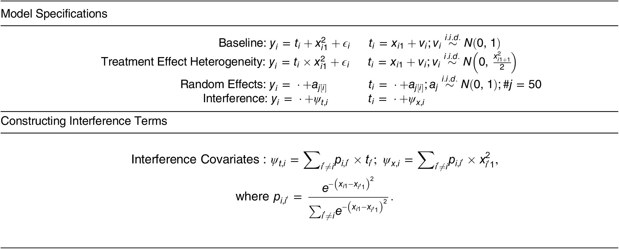
Note: The first simulation begins with the baseline additive model, and the second adds treatment effect heterogeneity bias by introducing a correlation between effect heterogeneity and treatment assignment heteroskedasticity. In the third, a fifty-leveled random effect is included as a confounder. The final specification adds an interference term, with the precise construction of the term at the bottom. The residual term $ {\varepsilon}_i $
follows a standard normal.
$ {\varepsilon}_i $
follows a standard normal.
The covariates are then transformed as
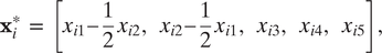 $$ {\mathbf{x}}_i^{\ast}\hskip0.35em =\hskip0.35em \left[{x}_{i1}-\frac{1}{2}{x}_{i2},\hskip0.33em {x}_{i2}-\frac{1}{2}{x}_{i1},\hskip0.33em {x}_{i3},\hskip0.33em {x}_{i4},\hskip0.33em {x}_{i5}\right], $$
and each method is given the outcome, treatment, transformed covariates, and indicator variables for the random effects regardless of whether the random effects are in the true data-generating process. I report results for n = 1,000, with additional sample sizes in Appendix F of the Supplementary Materials.Footnote 20
Along with the proposed method (PLCE), I implement four different machine learning methods. Kernel regularized least squares (KRLS; Hainmueller and Hazlett Reference Hainmueller and Hazlett2013) fits a single, nonparametric regression, takes the partial derivative of the fitted model with respect to the treatment variable, and returns the average of these values as the marginal effect. The covariate balancing propensity score for continuous treatments (CBPS; Fong, Hazlett, and Imai Reference Fong, Hazlett and Imai2018)Footnote
21 generates a set of weights that eliminate the effect of confounders under the assumption that the treatment distribution is normal and equivariant. I also include the double machine learning (DML) algorithm of Chernozhukov et al. (Reference Chernozhukov, Chetverikov, Demirer, Duflo, Hansen, Newey and Robins2018) with random forests used to learn $ \hat{f},\hskip2pt \hat{g} $
and the generalized random forest (GRF) of Athey, Tibshirani, and Wager (Reference Athey, Tibshirani and Wager2019), which is similar to DML but uses a particular random forest algorithm tuned for efficient inference on a marginal effect. Ordinary least squares (OLS) is included for comparison.
$ \hat{f},\hskip2pt \hat{g} $
and the generalized random forest (GRF) of Athey, Tibshirani, and Wager (Reference Athey, Tibshirani and Wager2019), which is similar to DML but uses a particular random forest algorithm tuned for efficient inference on a marginal effect. Ordinary least squares (OLS) is included for comparison.
The KRLS approach is closest to the proposed method in that both implement a nonparametric regression model. Thus, KRLS should handle nonlinearities well, but because it does not engage in a split-sample strategy, I expect undercoverage with its confidence intervals. The DML and GRF methods do engage in a split-sample strategy, but, like KRLS, they were not designed to handle random effects. I expect all three to perform poorly. Ordinary least squares should handle the random effects well, as they are simply entered as covariates in the model, but this should be particularly susceptible to treatment effect heterogeneity bias. None of the methods were constructed to adjust for interference. The proposed method, PLCE, should do a reasonable job across all settings, as it was designed to handle random effects and adjust for both interference and treatment effect heterogeneity bias.
Results for the Setting without Interference
The results for the simulations without interference are in Figure 2. The first column shows the distribution of point estimates, with the true value of $ 1 $
in gray. The second column shows the coverage rates: expected coverage is on the
$ 1 $
in gray. The second column shows the coverage rates: expected coverage is on the $ x $
-axis and actual coverage is on the
$ x $
-axis and actual coverage is on the $ y $
-axis.Footnote
22 For example, consider in the top right plot the point marked “
$ y $
-axis.Footnote
22 For example, consider in the top right plot the point marked “ $ \times $
” at
$ \times $
” at $ \left(\mathrm{0.90,0.85}\right) $
, which is on the CBPS curve. Here, I constructed a 90% confidence interval of the form
$ \left(\mathrm{0.90,0.85}\right) $
, which is on the CBPS curve. Here, I constructed a 90% confidence interval of the form $ \left[\hat{\theta}-1.64{\hat{\sigma}}_{\hat{\theta}},\hat{\theta}+1.64{\hat{\sigma}}_{\hat{\theta}}\right] $
and measured the proportion of simulations where the confidence interval contains the true value of 1. In this case, for CBPS, this value is 0.85, so the 90% confidence interval is invalid, albeit only slightly too narrow. More generally, if a curve falls below the 45° line, the confidence intervals are too narrow and thus invalid. If the curve falls above the 45° line, the confidence intervals are valid but wide.
$ \left[\hat{\theta}-1.64{\hat{\sigma}}_{\hat{\theta}},\hat{\theta}+1.64{\hat{\sigma}}_{\hat{\theta}}\right] $
and measured the proportion of simulations where the confidence interval contains the true value of 1. In this case, for CBPS, this value is 0.85, so the 90% confidence interval is invalid, albeit only slightly too narrow. More generally, if a curve falls below the 45° line, the confidence intervals are too narrow and thus invalid. If the curve falls above the 45° line, the confidence intervals are valid but wide.
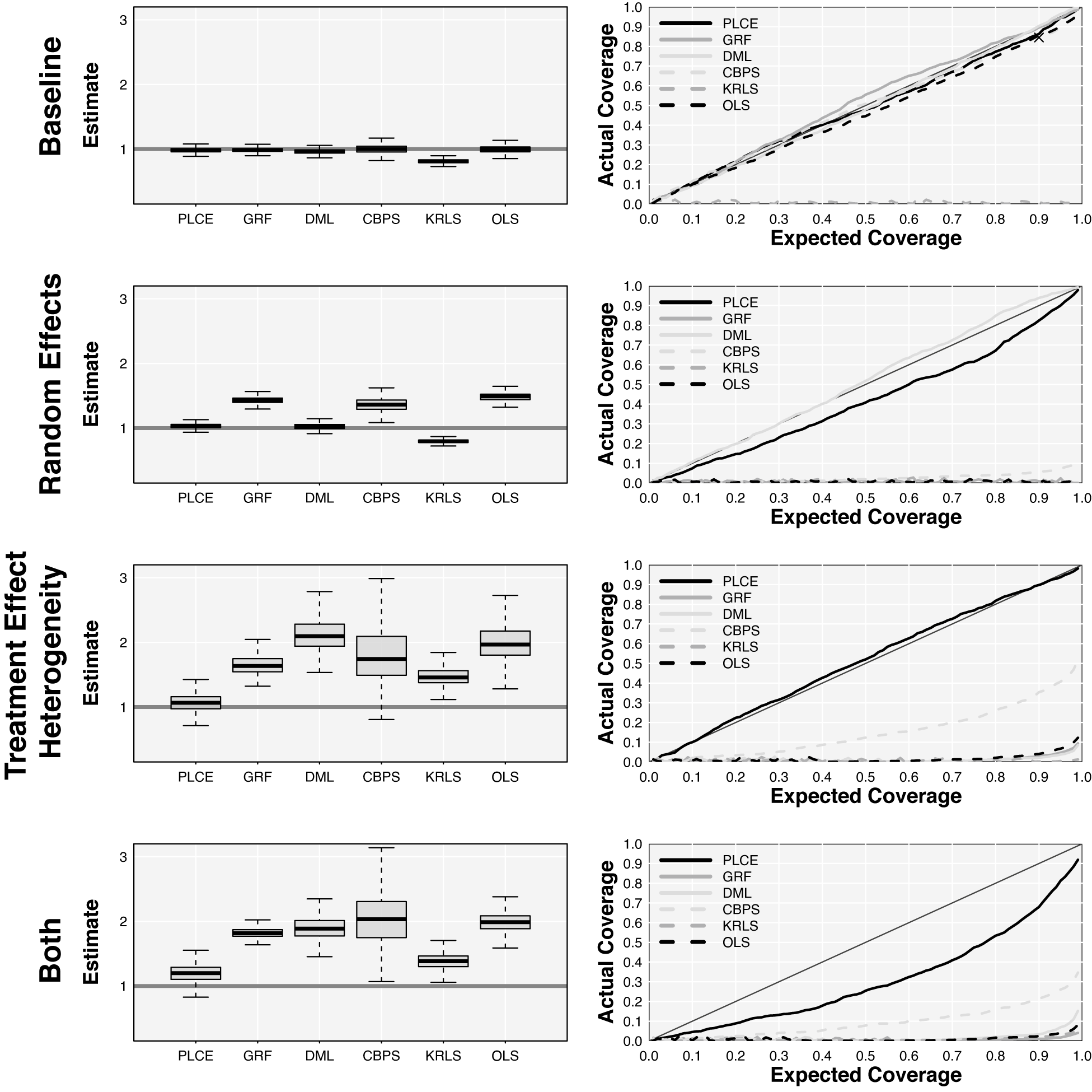
Figure 2. Results for Simulations without Interference
Note: The first column shows the distribution of point estimates, where the true value is $ 1 $
, in gray. The second column shows the coverage rates: expected coverage is on the
$ 1 $
, in gray. The second column shows the coverage rates: expected coverage is on the $ x $
-axis and actual coverage is on the
$ x $
-axis and actual coverage is on the $ y $
-axis. If a curve falls below the 45° line, the confidence intervals are too narrow and thus invalid. If the curve falls above the 45° line, the confidence intervals are valid but wide. The proposed method (PLCE) is compared with GRF, DML, CBPS, KRLS, and OLS. The proposed method, PLCE, is the only one to perform well across all settings.
$ y $
-axis. If a curve falls below the 45° line, the confidence intervals are too narrow and thus invalid. If the curve falls above the 45° line, the confidence intervals are valid but wide. The proposed method (PLCE) is compared with GRF, DML, CBPS, KRLS, and OLS. The proposed method, PLCE, is the only one to perform well across all settings.
The simulation settings increase in complexity going down the rows. The first row of figures contains contains the baseline model, the second, the model with group indicators added, the third, the baseline model with treatment effect heterogeneity, and the fourth, both treatment effect heterogeneity model and random effects.
Starting in the first row, every method performs well in the baseline model, though KRLS exhibits undercoverage. In the second row, with random effects added, only the proposed method and OLS provide unbiased estimates and valid inference. In the third row, the proposed method and KRLS are unbiased with valid intervals. In the final row, with both random effects and treatment effect heterogeneity, every method shows discernible bias, but the proposed method and KRLS have the lowest bias and the fewest misleading confidence errors.
Several machine learning methods fail to provide unbiased estimation in the presence of random effects or a simple interaction between the treatment effect and treatment residual. Across all settings, the proposed method is the only one that that allows for valid inference.
Results for the Setting with Interference
Figure 3 presents results from the simulations in the presence of interference. All methods save least squares return accurate point estimates in the simplest setting, with the proposed method, DML, and CBPS providing narrow but reasonable confidence intervals. Coverage from GRF, although valid in the setting without interference, is now near zero. In the remaining rows, the point estimates are reasonable, particularly for the proposed method but also KRLS. The effect of interference shows up in the coverage rates. In the bottom three settings, coverage rates are near zero for all methods. Only the proposed method provides both reliable point estimates and confidence intervals across each of the settings.

Figure 3. Results for Simulations with Interference
Note: The first column shows the distribution of point estimates, where the true value is 1, in gray. The second column shows the coverage rates: expected coverage is on the $ x $
-axis and actual coverage is on the
$ x $
-axis and actual coverage is on the $ y $
-axis. If a curve falls below the 45°, the confidence intervals are too narrow and thus invalid. If the curve falls above the 45° line, the confidence intervals are valid but wide. The proposed method (PLCE) is compared with GRF, DML, CBPS, KRLS, and OLS. The proposed method, PLCE, is the only one to perform well across all settings.
$ y $
-axis. If a curve falls below the 45°, the confidence intervals are too narrow and thus invalid. If the curve falls above the 45° line, the confidence intervals are valid but wide. The proposed method (PLCE) is compared with GRF, DML, CBPS, KRLS, and OLS. The proposed method, PLCE, is the only one to perform well across all settings.
Empirical Applications
I illustrate the proposed method using data from two recent studies. First, I reanalyze experimental data to illustrate that the proposed method returns estimates and standard errors similar to those from a linear regression when the linear regression is the correct thing to do. Second, I show how the method can estimate a treatment effect with a continuous treatment variable. I use data from a study where the researcher was forced to dichotomize a continuous treatment in order to estimate a causal effect.
Maintaining Efficiency
Mattes and Weeks (Reference Mattes and Jessica2019) conduct a survey experiment in the United States, asking respondents about a hypothetical foreign affairs crisis involving China and military presence in the Arctic. Varied is whether the hypothetical President is a hawk or dove, whether the policy is conciliatory or maintains status quo military levels, the party of the President, and whether the policy is effective in reducing Chinese military presence in the Arctic. The outcome is whether the respondent disapproves of the President’s behavior; controls consist of measures of the respondent’s hawkishness, views on internationalism, trust in other nations, previous vote, age, gender, education, party ID, ideology, interest in news, and importance of religion in their life.
I focus on how the estimated causal effect of conciliation varies between hawks and doves, as reported in Table 2 of the original work. The results appear in Table 3. For the two estimated effects, the proposed method returns results quite similar to those obtained with least squares. Importantly, the standard errors are comparable across the methods, suggesting no efficiency loss when employing the proposed method in a situation where least squares is known to be unbiased and efficient.
Table 3. Comparing PLCE and a Linear Regression in an Experimental Setting

Note: Across all settings, the PLCE estimates perform comparably to least squares on these experimental data. The repeated cross-fitting strategy does not inflate standard errors in this setting.
Estimating a Causal Effect in the Presence of a Continuous Treatment
I next reanalyze data from a recent study that estimated the causal effect of racial threat on voter turnout (Enos Reference Enos2016). The author operationalizes racial threat by distance to a public housing project, a continuous measure, and measures its effect on voting behavior. The demolishment of a subset of the projects in the early 2000s in Chicago provides a natural experiment used for identifying the causal effect. The author implements a difference-in-difference analysis that, unfortunately, requires a binary treatment. To accommodate the method, the author artificially dichotomizes the continuous treatment variable, considering all observations closer than some threshold distance to the projects as exposed to racial threat and observations further away as not. However, the threshold is not actually known, or even estimable, given the data. There is no reason to suspect that racial threat only extends, say, 0.3 kilometers, and drops off precipitously after. The proposed method allows estimation of the average causal effect of distance on the outcome.
I conduct four separate analyses. For the first, I estimate the causal effect of distance on change in turnout for white residents within one kilometer of a demolished housing project. The treatment variable is distance to the housing project, and the control variables consist of turnout in the previous two elections (1996, 1998), age, squared age, gender, median income for the Census block, value of dwelling place, and whether the deed for the residence is in the name of the voter. I also include a random effect for identifying the housing project nearest to each individual.Footnote 23 I next generate three matched samples for further analysis.Footnote 24 The first contains Black voters within one kilometer of a demolished housing project. As argued in the original piece (11), this group will not face racial threat, so it provides a measure of any trend in turnout absent racial threat. The next two samples consist of white and Black voters, but both are further than one kilometer from any housing project, either demolished or not. The latter two groups serve as placebo groups, as they are sufficiently far from a demolished project that any threat should be muted.
Figure 4 presents the effect estimates. I estimate that living adjacent to a public housing unit, rather than one kilometer away, causes a decrease in turnout of about $ 8.06 $
percentage points for white residents (
$ 8.06 $
percentage points for white residents ( $ SE\hskip0.35em =\hskip0.35em 0.0389,\hskip0.33em z\hskip0.35em =\hskip0.35em 2.07 $
), an effect in line with the results from the original analysis (see Figure 1 there). The estimated effect for Black voters near housing projects of
$ SE\hskip0.35em =\hskip0.35em 0.0389,\hskip0.33em z\hskip0.35em =\hskip0.35em 2.07 $
), an effect in line with the results from the original analysis (see Figure 1 there). The estimated effect for Black voters near housing projects of $ 0.017\hskip0.33em \left( SE\hskip0.35em =\hskip0.35em 0.035,\hskip0.33em z\hskip0.35em =\hskip0.35em 0.48\right) $
is not significant. The bottom two lines consider distal Blacks and whites, providing a placebo test. I find no effect of distance on turnout. Along with not relying on a user-specified control set, the proposed method allows for causal effect estimation with a continuous treatment variable. I find results of a magnitude similar to those from the original study but without needing to transform the data so that it is amenable to a framework that generally relies on a binary treatment.
$ 0.017\hskip0.33em \left( SE\hskip0.35em =\hskip0.35em 0.035,\hskip0.33em z\hskip0.35em =\hskip0.35em 0.48\right) $
is not significant. The bottom two lines consider distal Blacks and whites, providing a placebo test. I find no effect of distance on turnout. Along with not relying on a user-specified control set, the proposed method allows for causal effect estimation with a continuous treatment variable. I find results of a magnitude similar to those from the original study but without needing to transform the data so that it is amenable to a framework that generally relies on a binary treatment.
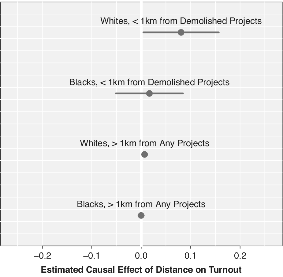
Figure 4. Causal Effect Estimate of Racial Threat
Note: Revisiting the study by Enos (Reference Enos2016), I find a statistically and substantively relevant effect of racial threat on white voters (top row) and, as predicted by theory, not for Black voters near the housing projects (second row) or for Black and white voters further than one kilometer from any projects.
Conclusion
Testing intuitions and hypotheses against the data in a way that does not rely on strong assumptions is essential to a reliable accumulation of knowledge. Doing so builds faith that the results and theory are driven by actual trends in the data and not a particular set of choices made by the researcher. To this end, I have introduced to political science a framework, taken from the field of semiparametric inference, for conducting valid inference while allowing machine learning methods to construct a control vector that can account for a wide range of commonly encountered biases. Essential to this approach is a sample-splitting strategy, where the same data is never used to both construct the control vector and conduct inference. I have extended this literature, allowing for inference that is robust to both heterogeneities in the treatment effect and particular patterns of interference among observations. The method extends causal inference, as well, accommodating continuous treatment variables. The accompanying software allows these analyses to be done in a line or two of code and allows for several diagnostics.
Ultimately, my goal is to allow for more believable, less assumption-driven inference. I move the field in this direction, where machine learning can be incorporated into workaday research as a means of controlling for background covariates, freeing the researcher to develop and test theories with some confidence that the results are not driven by her ability to specify every element of a statistical model.
SUPPLEMENTARY MATERIALS
To view supplementary material for this article, please visit http://doi.org/10.1017/S0003055422001022.
DATA AVAILABILITY STATEMENT
Research documentation and data that support the findings of this study are openly available at the American Political Science Review Dataverse: https://doi.org/10.7910/DVN/SWHIKY.
ACKNOWLEDGMENTS
I would like to thank Soichiro Yamauchi and Max Goplerud for work on developing the software; Dustin Tingley, Max Goplerud, John Londregan, Scott de Marchi, Brandon Stewart, Kevin Munger, Curtis Signorino, Christopher Lucas, Matt Blackwell, Dean Knox, Neal Beck, Cyrus Samii, Matias Cattaneo, Rod Little, Walter Mebane, and Jonathan Katz, for helpful comments; Camille DeJarnett for excellent research assistance; and Stefan Wager for guidance in implementing his software.
CONFLICT OF INTEREST
The author declares no ethical issues or conflicts of interest in this research.
ETHICAL STANDARDS
The author affirms that this research did not involve human subjects.


 Open access
Comments
No Comments have been published for this article.