


Introduction
The advent of modern biotechnologies, bio-sensing hardware, and information technology infrastructure mark the beginning of an ever-increasing high-throughput data collection livestock management era that pushes the development of computationally more efficient and faster methods to supreme levels. Animal breeding makes no exception and it is currently facing a methodological and conceptual transition to a colloquially called ‘big data era’. While traditional information sources for animal breeding included phenotype and pedigree information, nowadays there is a large influx of genomic data consisting of single nucleotide polymorphisms (SNPs), gene annotations, metabolic pathways, protein interaction networks, gene expression, and protein structure information that could potentially be used to improve the reliability of genetic predictions and further the understanding of phenotypes biology.
The livestock industry has also been under major technological changes in genetic selection, herd and operations management, and more importantly automated sensor-based data collection in the last decade. Sensor technology has a big potential to increase production efficiency by monitoring the activity of animals in large herds and by sending alerts for health and fertility events or collecting expensive-to-measure phenotypes. Such large data collections in combination with other sources of data (e.g. genomic) bring an opportunity to create predictive models for health, fertility, and other traits or events.
While the integration of such heterogeneous information in several bio-medical areas has been proven successful for the past 15 years, it is still in its infancy in animal breeding (Pérez-Enciso, Reference Pérez-Enciso2017). The integration of large genome data, such as SNP markers, in animal breeding is typically hampered by the lack of sufficient observations, N, and the deluge of predictive variables, P (also known as the ‘large P, small N’ paradigm or the ‘curse of dimensionality’). Complex relationships hidden within large, noisy, and redundant data are hard to unravel using traditional linear models. This requires the application of nonparametric models from the machine learning (ML) repository, which is known to be particularly fit for addressing these problems.
The availability of exponentially increasing information of mixed content (homogeneous and heterogeneous) and a concomitant boost in computational processing power lead to the development of more advanced ML approaches and to the ‘rediscovery’ of the utility of specific types of artificial neural network (ANN) methods that form a special class called ‘deep learning’. ML techniques such as deep learning (DL) can greatly help to extract pattern and similarity relationships when traditional models fail to handle and model big data with complex data structures. Similarly, advanced Artificial Intelligence (AI) methods can drastically change herd management processes by providing solid evidence leading to informed decisions using real-time data collection from various types of sensors (electro-optical, audio, etc.).
This article provides a succinct description of traditional and novel prediction methods used in animal breeding to date and sheds light on potential trends and new research directions that could change the landscape of livestock management in a digital future.
Traditional animal breeding prediction methods
Quantitative or complex traits (including milk production and fertility traits) are influenced by many genes (>100 to thousands) with small individual effects (Glazier et al., Reference Glazier, Nadeau and Aitman2002; Schork et al., Reference Schork, Thompson, Pham, Torkamani, Roddey, Sullivan, Kelsoe, O'Donovan, Furberg, Schork, Andreassen and Dale2013). Selection for these traits was first based on phenotype and pedigree information and the knowledge of the genetic parameters for the trait of interest (Dekkers and Hospital, Reference Dekkers and Hospital2002).
The best linear unbiased prediction (BLUP) model
One of the most widely used models, the BLUP mixed linear model (Henderson, Reference Henderson1985; Lynch and Walsh, Reference Lynch and Walsh1998) was implemented on extensive databases of recorded phenotypes for the trait of interest or their correlated traits to estimate the breeding value (EBV) of selection candidates (Dekkers, Reference Dekkers2012). The accuracy of this method is defined as the correlation between the true and estimated breeding value and is one of the determinants of the rate of genetic improvement in a breeding program per unit of time (Falconer et al., Reference Falconer, Douglas and Mackay1996). The success rate of selection programs based on EBV estimated from phenotype was high; however, it was accompanied by a number of limitations including the need for routinely recording phenotypes on selection candidates or their relatives in a timely manner and at early ages. Additionally, some traits of interest are only recorded late in life (e.g. longevity) or are either limited by the sex of the animal (e.g. milk yield in dairy cattle, semen for bulls), difficult to measure (e.g. disease resistance) or require animals to be sacrificed (e.g. meat quality). Subsequently, these phenotyping constraints pose serious limitations to genetic progress (Dekkers, Reference Dekkers2012).
Single-step genomic best linear unbiased prediction (ssGBLUP)
Currently, the genomic best linear unbiased prediction (GBLUP) model is used in a two-step (or multi-step) approach for genomic predictions (Misztal, Reference Misztal2016). This implies running the regular BLUP evaluation to compute EBVs. Then the EBVs are de-regressed (dEBV) to extract the pseudo-observations for genotyped individuals and are eventually used as input variables for genomic predictions (Misztal et al., Reference Misztal, Legarra and Aguilar2009; Misztal et al., Reference Misztal, Aggrey and Muir2013; National Genomic Evaluations Info –Interbull Centre, 2019). However, using the genetic relation matrix (G) for genomic selection (GS) through a two-step methodology is complicated and includes several approximations (Misztal et al., Reference Misztal, Aggrey and Muir2013). Pseudo-observations are dependent on other estimated effects and approximate accuracy of EBVs. All the approximations reduce the accuracy of EBVs, which subsequently can inflate the genomic breeding values (GEBVs) (Misztal et al., Reference Misztal, Legarra and Aguilar2009). Furthermore, the availability of genotype information on only a limited proportion of animals in some developing countries has promoted the implementation of the single-step methodology (ssGBLUP) (Misztal et al., Reference Misztal, Legarra and Aguilar2009). In this model, pedigree and genomic relationships are combined into an H matrix to predict the genetic merit of the animal, which results in higher accuracy due to the utilization of all the available data (Misztal et al., Reference Misztal, Legarra and Aguilar2009; Cardoso et al., Reference Cardoso, Gomes, Sollero, Oliveira, Roso, Piccoli, Higa, Yokoo, Caetano and Aguilar2015; Valente et al., Reference Valente, Baldi, Sant'Anna, Albuquerque and Paranhos da Costa2016). Aguilar et al. (Reference Aguilar, Misztal, Johnson, Legarra, Tsuruta and Lawlor2010) showed that a single-step methodology can be simple, fast, and accurate.
Quantitative trait loci (QTL) mapping and marker-assisted selection (MAS)
Improvement in molecular genetics provided new opportunities to enhance breeding programs for selected candidates through the application of DNA markers and the identification of genomic regions (QTL) that control the trait of interest (Dekkers, Reference Dekkers2012). In earlier QTL mapping studies, sparse genetic markers and linkage disequilibrium (LD) analysis were used to identify genes and markers that can be implemented in breeding programs via MAS (Weller et al., Reference Weller, Kashi and Soller1990; Dekkers, Reference Dekkers2004). MAS increased the rate of genetic gain especially when the traditional selection was less effective (Spelman et al., Reference Spelman, Coppieters, Grisart, Blott and Georges2001; Abdel-Azim and Freeman, Reference Abdel-Azim and Freeman2002). Additionally, these analyses resulted in the discovery of a great number of QTLs and marker-phenotype associations, and identification of some causative mutations (Andersson, Reference Andersson2001; Dekkers and Hospital, Reference Dekkers and Hospital2002; Dekkers, Reference Dekkers2004). However, the success of these selections was limited mainly due to the very small variance explained by the identified QTLs (Schmid and Bennewitz, Reference Schmid and Bennewitz2017).
The advent of high-density genotyping panels and Whole-Genome Selection continue the advancement of molecular genetic technologies (Meuwissen et al., Reference Meuwissen, Hayes and Goddard2001; Matukumalli et al., Reference Matukumalli, Lawley, Schnabel, Taylor, Allan, Heaton, O'Connell, Moore, Smith, Sonstegard and Van Tassell2009; Dekkers, Reference Dekkers2012), and in conjunction with bovine SNP discovery and sequencing projects (Bovine HapMap Consortium et al., Reference Gibbs, Taylor, Van Tassell, Barendse, Eversole, Gill, Green, Hamernik, Kappes, Lien, Matukumalli, McEwan, Nazareth, Schnabel, Weinstock, Wheeler, Ajmone-Marsan, Boettcher, Caetano, Garcia, Hanotte, Mariani, Skow, Sonstegard, Williams, Diallo, Hailemariam, Martinez, Morris, Silva, Spelman, Mulatu, Zhao, Abbey, Agaba, Araujo, Bunch, Burton, Gorni, Olivier, Harrison, Luff, Machado, Mwakaya, Plastow, Sim, Smith, Thomas, Valentini, Williams, Womack, Woolliams, Liu, Qin, Worley, Gao, Jiang, Moore, Ren, Song, Bustamante, Hernandez, Muzny, Patil, San Lucas, Fu, Kent, Vega, Matukumalli, McWilliam, Sclep, Bryc, Choi, Gao, Grefenstette, Murdoch, Stella, Villa-Angulo, Wright, Aerts, Jann, Negrini, Goddard, Hayes, Bradley, Barbosa da Silva, Lau, Liu, Lynn, Panzitta and Dodds2009; Stothard et al., Reference Stothard, Choi, Basu, Sumner-Thomson, Meng, Liao and Moore2011; Daetwyler et al., Reference Daetwyler, Capitan, Pausch, Stothard, van Binsbergen, Brøndum, Liao, Djari, Rodriguez, Grohs, Esquerré, Bouchez, Rossignol, Klopp, Rocha, Fritz, Eggen, Bowman, Coote, Chamberlain, Anderson, VanTassell, Hulsegge, Goddard, Guldbrandtsen, Lund, Veerkamp, Boichard, Fries and Hayes2014), have led to availability of high-density SNP arrays for most livestock species and the application of GS. Meuwissen et al. (Reference Meuwissen, Hayes and Goddard2001) transferred marker-assisted selection on a genome-wide scale and developed statistical models to estimate GEBVs that rely on genome-wide dense markers. The first high-density genotyping panel available for livestock was the 50 K Bovine Illumina SNP platform (Matukumalli et al., Reference Matukumalli, Lawley, Schnabel, Taylor, Allan, Heaton, O'Connell, Moore, Smith, Sonstegard and Van Tassell2009). This SNP panel has been since widely used in genotyping dairy and beef cattle bulls and similar SNP panels of between 40 and 65 thousand SNPs are now available for other livestock species (Dekkers, Reference Dekkers2012). Higher density chips became available in cattle in 2010 (e.g. the BovineHD beadchip from Illumina) covering 777,000 markers and such higher density panels are also under development in other species (Matukumalli et al., Reference Matukumalli, Lawley, Schnabel, Taylor, Allan, Heaton, O'Connell, Moore, Smith, Sonstegard and Van Tassell2009). To calculate GEBVs, first all SNPs are fit simultaneously in the models with their effects considered as random variables and then the effects of markers (mostly in the form of SNPs) are estimated in a reference population (consisting of animals that are genotyped and phenotyped for the traits of interest). These effects are used to build a prediction equation that is then applied to a second population, consisting of selection candidates, for which the genotype information is available while the phenotype information is not necessarily known. The estimated effects of the markers that each animal carries are summed across the whole genome to calculate the GEBV (Meuwissen et al., Reference Meuwissen, Hayes and Goddard2001; Hayes et al., Reference Hayes, Bowman, Chamberlain, Verbyla and Goddard2009) representing the genetic merit of the individual (Meuwissen and Goddard, Reference Meuwissen and Goddard2007). The GS approach can increase the accuracy of selection (Meuwissen et al., Reference Meuwissen, Hayes and Goddard2001; Schaeffer, Reference Schaeffer2006) and can reduce generation intervals. Many statistical models and approaches have been proposed for genomic predictions. These models can be classified broadly into linear and non-linear methods (Daetwyler et al., Reference Daetwyler, Pong-Wong, Villanueva and Woolliams2010). GBLUP is an example of a linear model while the Bayesian approaches such as Bayes-(A/B/C/etc.) using Monte Carlo Markov Chain (MCMC) methodology are examples of non-linear methods (Gianola et al., Reference Gianola, de los Campos, Hill, Manfredi and Fernando2009; Habier et al., Reference Habier, Fernando, Kizilkaya and Garrick2011). The major difference between these two methods is their prior assumptions about the effect of SNPs as explained in Neves et al. (Reference Neves, Carvalheiro and Queiroz2012) and Campos et al. (Reference Campos, Hickey, Pong-Wong, Daetwyler and Calus2013). The GBLUP assumption states that the genetic variation for the trait is equally distributed across all SNPs on the genotyping panel, similar to the infinitesimal model of quantitative genetics (Strandén and Garrick, Reference Strandén and Garrick2009). The GBLUP model is more commonly used in routine genomic evaluations where high-density SNP genotypes can be used to construct a genomic relationship matrix (G) among all individuals in the population and the G matrix is used instead of the traditional pedigree-based relationship matrix (A) in the BLUP model (Habier et al., Reference Habier, Fernando and Dekkers2007; Ødegård and Meuwissen, Reference Ødegård and Meuwissen2014, Reference Ødegård and Meuwissen2015). Bayesian methods are different in the adoption of priors while sharing the same sampling model (Zhu et al., Reference Yu, Pressoir, Briggs, Vroh Bi, Yamasaki, Doebley, McMullen, Gaut, Nielsen, Holland, Kresovich and Buckler2016). For example, BayesA assumes all SNPs have effects and each SNP has its own variance while the prior distribution of SNP effects in BayesB are assumed zero with probability of π, and normally distributed with a zero mean and locus specific variance with probability (1−π) (Meuwissen et al., Reference Meuwissen, Hayes and Goddard2001). Bayesian methods that are implemented using MCMC algorithms are time-consuming and computationally demanding when they handle large number of SNPs. Therefore, several iterative (non-MCMC-based Bayesian) methods such as VanRaden's non-linear A/B (VanRaden, Reference VanRaden2008), fastBayesB (Meuwissen et al., Reference Meuwissen, Solberg, Shepherd and Woolliams2009), MixP (Yu and Meuwissen, Reference Yu and Meuwissen2011) or emBayesR (Habier et al., Reference Habier, Fernando and Dekkers2007) were developed to overcome the computational demands (Iheshiulor et al., Reference Iheshiulor, Woolliams, Svendsen, Solberg and Meuwissen2017). The aforementioned methods are computationally fast, and they result in prediction accuracies similar to those of the MCMC-based methods. Compared to GBLUP, non-linear methods can better exploit the LD information gained through mapping of QTLs (Habier et al., Reference Habier, Fernando and Dekkers2007). The result of investigations, however, have indicated that GBLUP is generally as accurate as Bayes-A/B/C procedures (Hayes et al., Reference Hayes, Bowman, Chamberlain, Verbyla and Goddard2009; VanRaden et al., Reference VanRaden, Van Tassell, Wiggans, Sonstegard, Schnabel, Taylor and Schenkel2009). This implies that the number of QTLs is high and the infinitesimal model is approximately correct for most traits (Daetwyler et al., Reference Daetwyler, Pong-Wong, Villanueva and Woolliams2010). Therefore, an increase in the accuracy of GS mainly results from a better and more accurate estimation of the genomic relation matrix (G) among animals rather than by estimating effects of major genes such as using Bayesian models (Misztal et al., Reference Misztal, Aggrey and Muir2013).
Genome-wide association studies (GWAS)
A large amount of high-density SNP data generated from genomic sequencing technologies can be also used in GWAS to identify genetic markers or genomic regions associated with the traits of interest based on population-wide Linkage-Disequilibrium (LD). These associations are due to the existence of small segments of chromosomes in the current population that descended from a common ancestor (Hayes, Reference Hayes2013). Researchers have used a number of different statistical methodologies to exploit these associations. These methods included single-SNP GWAS analysis, haplotype GWAS analysis, the Identical By Descent approach, and GWAS analysis fitting all markers simultaneously (Hoggart et al., Reference Hoggart, Whittaker, De Iorio and Balding2008; Hayes, Reference Hayes2013; Wu et al., Reference Wu, Fan, Wang, Zhang, Gao, Chen, Li, Ren and Gao2014; Richardson et al., Reference Richardson, Berry, Wiencko, Higgins, More, McClure, Lynn and Bradley2016; Abo-Ismail et al., Reference Abo-Ismail, Brito, Miller, Sargolzaei, Grossi, Moore, Plastow, Stothard, Nayeri and Schenkel2017; Akanno et al., Reference Akanno, Chen, Abo-Ismail, Crowley, Wang, Li, Basarab, MacNeil and Plastow2018; Chen et al., Reference Chen, Yao, Ma, Wang and Pan2018; do Nascimento et al., Reference do Nascimento, da Romero, Utsunomiya, Utsunomiya, Cardoso, Neves, Carvalheiro, Garcia and Grisolia2018). The GWAS method, however, comes with its own challenges. For example, in the single marker regression model, one SNP at a time is fitted as a fixed effect in a BLUP animal model to account for the family structure of the data by fitting a polygenic effect with pedigree-based relationships (Kennedy et al., Reference Kennedy, Quinton and van Arendonk1992; Mai et al., Reference Mai, Sahana, Christiansen and Guldbrandtsen2010; Cole et al., Reference Cole, Wiggans, Ma, Sonstegard, Lawlor, Crooker, Van Tassell, Yang, Wang, Matukumalli and Da2011). This model is accompanied by several disadvantages such as the marker effect overestimation due to multiple testing and the single SNP approach relying on the pairwise LD of a QTL with individual SNPs. Therefore, a region containing the true mutation can be hard to find, as a large number of SNPs can be in LD with the QTL (Pryce et al., Reference Pryce, Goddard, Raadsma and Hayes2010). Population structure or relatedness between individuals can result in a high rate of false positives (FP), a lower mapping precision and lower statistical power (Li et al., Reference Li, Su, Jiang and Bao2017). The Linear Mixed Model (LMM) is an effective method to handle population structure (Yu et al., Reference Yu, Pressoir, Briggs, Vroh Bi, Yamasaki, Doebley, McMullen, Gaut, Nielsen, Holland, Kresovich and Buckler2006), though computationally demanding. The best solution to overcome these issues is to fit all the SNPs simultaneously, which involves using the same models that have been proposed for genomic predictions (Meuwissen et al., Reference Meuwissen, Hayes and Goddard2001; Hayes, Reference Hayes2013). In this model, the SNP effect is fit randomly (derived from a distribution) with different prior assumptions on the distribution of possible SNP effects via SNPBLUP or ridge regression (Meuwissen et al., Reference Meuwissen, Hayes and Goddard2001), BayesA (Meuwissen et al., Reference Meuwissen, Hayes and Goddard2001; Gianola et al., Reference Gianola, Hayes, Goddard, Sorensen and Calus2013), Bayes SSVS (Verbyla et al., Reference Verbyla, Hayes, Bowman and Goddard2009, Reference Verbyla, Bowman, Hayes and Goddard2010), BayesCπ (Habier et al., Reference Habier, Fernando, Kizilkaya and Garrick2011), and BayesR (Erbe et al., Reference Erbe, Hayes, Matukumalli, Goswami, Bowman, Reich, Mason and Goddard2012). These methods have been used in several GWAS studies (Veerkamp et al., Reference Veerkamp, Verbyla, Mulder and Calus2010; Kizilkaya et al., Reference Kizilkaya, Tait, Garrick, Fernando and Reecy2011; Sun et al., Reference Sun, Fernando, Garrick and Dekkers2011; Peters et al., Reference Peters, Kizilkaya, Garrick, Fernando, Reecy, Weaber, Silver and Thomas2012) with priors of multiple normal distributions and different SNP classifications on the basis of their posterior probabilities of being in each distribution as zero effect or small effect (Erbe et al., Reference Erbe, Hayes, Matukumalli, Goswami, Bowman, Reich, Mason and Goddard2012).
Although the available technologies have revolutionized the paradigm of the prediction of genetic merit or phenotypes of individuals (Campos et al., Reference Campos, Hickey, Pong-Wong, Daetwyler and Calus2013), serious over-fitting problems may be encountered where the ratio between the number of variables (P) and the number of observations (N) exceeds 50–100. Additionally, in genomic predictions, there is still an issue on whether or not all SNPs should be included in a predictive model. For example, in an association analysis, the exclusion of irrelevant SNPs led to a more accurate classification (Long et al., Reference Long, Gianola, Rosa, Weigel and Avendaño2007). ML is an alternative approach for prediction, classification, and dealing with the ‘curse of dimensionality’ problem in a flexible manner (González-Recio et al., Reference González-Recio, Rosa and Gianola2014). Compared with Bayesian models, ML approaches may provide larger and more general flexible methods for regularization by assigning different prior distributions to marker effects. There has been a number of studies using various ML methods including Support Vector Machines (SVMs), Random Forests (RF), Boosting, and ANNs applied to livestock data that will be introduced and presented in detail in the next sections.
ML prediction and evaluation methods
A large number of ML approaches were developed since the early 1960s and they had a significant impact on various types of problems, such as regression, classification, clustering, and dimensionality reduction (Fig. 1) from multiple areas of studies. We provide below a short description of a handful of such methods (listed alphabetically) and we describe their successful application in livestock studies in the next section.
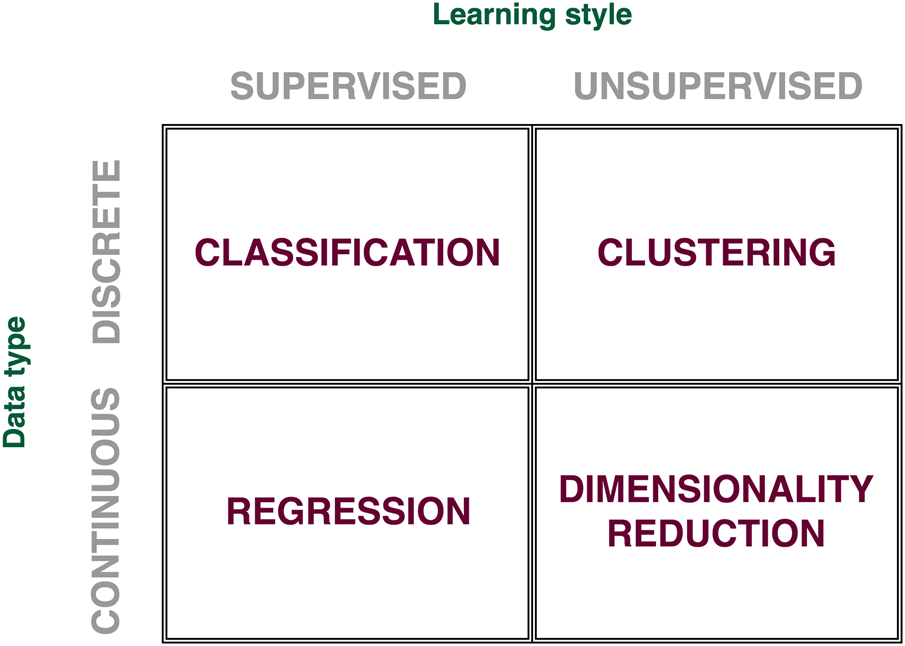
Fig. 1. Types of machine learning problems. Based on data type (discrete and continuous) and learning style (supervised and unsupervised), machine learning problems can be grouped into four main classes: classification, clustering, regression, and dimensionality reduction.
Artificial neural networks
ANNs represent a group of biologically inspired models frequently employed by computational scientists for prediction and classification problems. Typically, an ANN consists of one or more layers of interconnected computational units called neurons.
A neuron is typically represented as a summation function upon which an activation function is applied (Fig. 2). The neuron receives one or more separately weighted inputs and a bias, which in turn are summed up and represent the activation potential of the neuron. The sum is then passed as argument to an activation function typically having a sigmoid shape. They represent a thresholding approach that allows only strong signals to be further transmitted to other neurons. The connection strength among neurons is represented by weights and the weights get updated during the training stage of an ANN. The training stage of an ANN consists of presenting the network with a set of inputs for which the desired output is known, and the learning aspect is realized by minimizing the differences between the calculated and desired outputs. The weights and biases of an ANN are typically initialized by drawing values from a random normal distribution. A popular algorithm that allows the propagation of error back through the network and the continuous update of weights and biases is called backpropagation and was proposed in 1986 (Rumelhart et al., Reference Rumelhart, Hinton and Williams1986). The main advantages of ANNs are their ability to learn and model non-linear and complex systems, the ability to generalize from limited amounts of data, and their lack of restrictions with respect to input variables (e.g. no assumptions about their distribution).
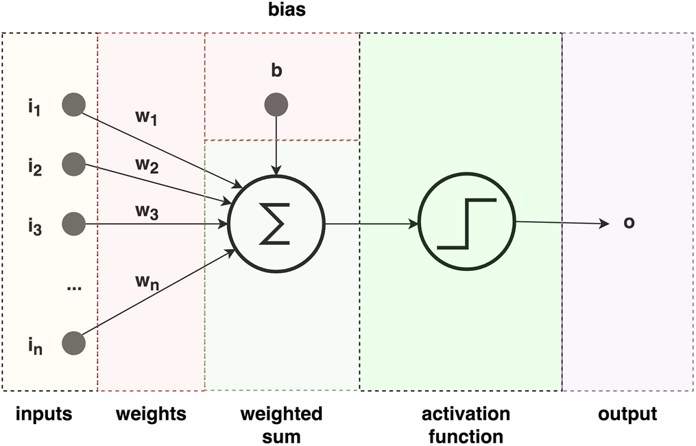
Fig. 2. Schematic representation of an artificial neuron. An artificial neuron has five main parts: inputs i 1…n, weights w 1…n (and bias b), a summation function, an activation function (typically defined as a sigmoid), and output.
Bagging or bootstrap aggregation (BA)
BA or bagging (Breiman, Reference Breiman1996) is a simple and efficient ensemble method that combines the prediction of multiple ML algorithms to make more accurate predictions. It works particularly well when the individual ML algorithms have a high prediction variance such as decision trees (DT). The aggregation of predictions constitutes either the average of numeric values or the majority of predicted non-numeric class labels. Its main purpose is to boost up the robustness of predictors for problem sets where small variations in the data cause significant changes in predictions. In principle, BA improves prediction accuracy by bootstrapping the initial training step multiple times and then training various ML models on each training subset. The results are either averaged out if numeric or a majority voting principle is applied to identify the majority class.
Decision trees
DT are data structures that use nodes and edges to represent a problem. Internal nodes in a tree represent attribute tests while terminal nodes represent the answers to such tests. Branches are used to connect two nodes in a DT and model the possible outcomes of an attribute test. In ML, DT are among the most intuitive and simplest to interpret models and widely used for classification and prediction problems. While the overall architecture of a DT is highly dependent on small changes in the input data, they are very flexible means to represent mixed data (categorical and numerical) and data with missing features. While DT are particularly well fit to represent classification problems, they can be easily modified to represent regression problems and, once constructed, they are among the fastest ML approaches for classification problems. A more succinct description of DT can be found in Kingsford and Salzberg (Reference Kingsford and Salzberg2008).
Deep learning
DL is a subset of ANN-based ML techniques that have been recently applied predominantly on previously computationally hard classification problems in natural language processing and computer vision. Based on ANNs with multiple processing layers and using backpropagation for training, DL makes use of recent advancements in hardware technology (better CPUs, extended RAM and storage space) to make such ANNs computationally efficient for solving classification problems that require very large data sets. Major breakthroughs in object recognition, image classification and speech and audio processing were achieved when convolutional neural networks and recurrent nets were used. A detailed description of DL approaches and their results can be found in (LeCun et al., Reference LeCun, Bengio and Hinton2015).
eXtreme gradient boosting (XgBoost)
Yet another ensemble method, the XgBoost method (Chen and Guestrin, Reference Chen and Guestrin2016) is an implementation of the gradient boosting machines (GBMs) that is focused on computational speed and model performance. The additional performance is achieved with the aid of an efficient linear model solver and a tree learning algorithm combined with parallel and distributed computing and efficient memory usage. The method is typically used to solve regression and classification problems and it is also heavily used for ranking tasks.
Gradient boosting machine
GBM is a ML approach that combines the gradient descent error minimization approach with boosting and fits new models with the overall goal to more accurately estimate the desired response. Boosting is typically used in ML to convert weak prediction models (typically referred to as ‘weak learners’) into stronger ones.
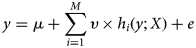 $$y = \mu + \mathop \sum \limits_{i = 1}^M \upsilon \times h_i(y;X) + e$$
where y is the vector of observed data (e.g. phenotypes), μ is the population mean, υ is a shrinkage factor, h i is a prediction model, X is a matrix (e.g. corresponding genotypes), and e is a vector of residuals.
GBM is applicable to classification and regression problems and encapsulates an ensemble of weak prediction models. While traditional ensemble ML techniques such as RF rely on averaging of model predictions in the ensemble, GBM adds new models to the ensemble sequentially. At each step, a new weak learner is added and trained with respect to the error of the whole ensemble learnt up to this point such that the newly added model is maximally correlated with the negative gradient of the loss function, associated with the whole ensemble. Examples of successful GBMs include AdaBoost (Freund and Schapire, Reference Freund and Schapire1997), RF (Breiman, Reference Breiman2001), and XGBoost (Chen and Guestrin, Reference Chen and Guestrin2016). A more detailed description of GBMs can be found in Natekin and Knoll (Reference Natekin and Knoll2013).
Naïve Bayes (NB)
NB (Clark and Niblett, Reference Clark and Niblett1989) is an inductive learning algorithm widely used in ML (classification, regression, prediction) and data mining due to its simplicity, computational efficiency, robustness, and linear training time directly proportional with the number of training examples. The algorithm uses the Bayes rule (Bayes, Reference Bayes1763) and strong independence assumptions about the attributes of the class. The NB classifier assumes that the effect of the value of a predictor (x) on a given class (c) is independent of the values of the other predictors. The NB algorithm uses the information from training data to estimate the posterior probability P(c|x) of each class c, given an object x, which subsequently can be used to classify other objects. According to Bayes theorem:
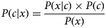 $$P(c{\rm \vert} x) = \displaystyle{{P(x{\rm \vert} c) \times P(c)} \over {P(x)}}$$
where P(c|x) is the posterior probability of class c given predictor x, P(x|c) represents the likelihood, i.e. the probability of predictor x given class c, P(c) is the prior probability of class c and P(x) is the probability of predictor x.
Given the class conditional independence assumption for NB, the posterior probability can be expressed as follows:
 $$P(c{\rm \vert} x) = P(x_1{\rm \vert} c) \times P(x_2{\rm \vert} c) \times P(x_3{\rm \vert} c) \times \ldots \times P(x_n{\rm \vert} c) \times P(c)$$
where x i with i = 1:n represent all the features in predictor x.
While in practice the attributes of a class are not always independent, the NB algorithm can tolerate a certain level of dependency between variables and can easily outperform more complex methods such as DT and rule-based classifiers on various classification problems (Ashari et al., Reference Ashari, Paryudi and Min2013), while it is easily outperformed by other methods on regression problems (Frank et al., Reference Frank, Trigg, Holmes and Witten2000).
Partial least squares regression (PLSR)
The PSLR method (also known as the Projection to Latent Structures Regression method) was developed in the early 1960s by Herman Wold and his son as an econometric technique, but it becomes quickly adopted as a state-of-the-art technique in chemometrics and other engineering areas. The method is typically used to construct predictive models when there are many highly colinear (high redundancy) variables describing the problem to be solved. In such particular case multiple linear regression is not applicable and PLSR becomes the method of choice. The method's focus is on prediction and not on underlying the intrinsic relationships between variables or reducing their number.
Random forests (RF)
Originally proposed by Reference Tin Kam HoTin Kam Ho (1995) and later perfected by Breiman (Breiman, Reference Breiman2001), a RF is an ensemble-based ML technique that uses multiple DT and Bootstrap Aggregation (BA) to perform classification or regression tasks. Multiple sampling with replacement is performed on the data and a DT is trained on each sample. In essence, the DT approach relies on the complementary generalization capability of multiple DT built on randomly selected subspaces of the whole data feature space and the ability to improve the classification power of the whole ensemble of models. While the interpretability of the models obtained with RFs is less than ideal, a great advantage of RFs is their robustness and ability to handle missing data, which is a predominant factor in biological studies.
Reproducing Kernel Hilbert spaces (RKHS)
A Hilbert space is typically defined as a generalization of an Euclidian space where vector algebra and calculus can be applied on mathematical spaces with more than 2 or 3 dimensions. In retrospective, a RKHS is a Hilbert space of functions where two functions, f and g, with close norms (∥f − g∥ → 0) are also close in their values (|f(x) − g(x) → 0|), which is equivalent of saying that the Hilbert space has bounded and continuous functionals. The RKHS theory can be successfully applied to three main types of problems as suggested by Manton and Amblard (Reference Manton and Amblard2014). The first type of problems suggests that if a problem is defined over a subspace that is proven to be RKHS, the properties of the RKHS will help with solving that problem. This implies that sometimes, problem space can be mapped onto a different space where the problem becomes easier solvable. The second type of problems refers to those that have positive semi-definite functions, which can be solved by introducing an RKHS with a kernel that is equivalent to the positive semi-definite functions. The third type of problem refers to those situations where, given all the data points and a function defining the distance between them, the points can be embedded into an RKHS with the kernel function capturing the properties of the distance function. Overall, RKHS can help solving problems where problems in one space become easier to solve in a different space and the optimality of their solutions remains unchanged in both spaces (Berlinet and Thomas-Agnan, Reference Berlinet and Thomas-Agnan2004).
Rotation forests (ROF)
Introduced in 2006 by Rodriguez et al. (Reference Rodriguez, Kuncheva and Alonso2006), ROF constitute a method for generating an ensemble of classifiers relying on extraction of better features with the aid of the Principal Component Analysis method after the training data is split into a fixed number of subsets (K). The resulting principal components obtained after K-axis rotations will then serve as new features for the base DT classifiers (thus the name ‘forest’), which are trained on the whole data, thus maintain high accuracy and diversity within the ensemble. Preliminary results showed that ROF ensembles contain more accurate individual classifiers compared with AdaBoost and RF and more diverse than the ones obtained with bagging techniques.
Support vector machines
Proposed in 2001 (Ben-Hur et al., Reference Ben-Hur, Horn, Siegelmann and Vapnik2001), SVM is a supervised ML approach predominantly used to solve classification problems. However, it is also used successfully to solve regression problems. SVMs function based on the notions of dimension separability by decision planes and boundaries and rely on construction of multidimensional hyperplanes that separate similarly grouped/labeled items into linearly separable sets. SVMs can handle both, categorical (discrete) and numeric (continuous) variables. The construction of optimal hyperplanes is performed by an iterative training algorithm used to minimize an error function. SVMs use kernels to map the original objects into a new space described by support vectors (coordinates of objects), which make the separability task feasible. SVMs are effective methods when applied to non-linearly separable data with a high number of dimensions, particularly for ‘small n, large p’, problems where the number of dimensions (p) is higher than the number of observations (n). SVM is memory efficient since it is using a subset of the training data points to build the support vectors. Nevertheless, SVM is not computationally efficient when applied to very large data sets since the required training time is high. Also, SVM tends to perform poorly when the data is noisy, and the classes or labels are overlapping.
ML evaluation methods
The evaluation of ML methods is a very important part of any project employing such approaches and it is very important to choose the right metrics to measure their performance. Below we enumerate some of the most used evaluation methods in the ML field. Most of the metrics rely on the definition of a confusion matrix, where true and false positives and negatives (TP, TN, FP, FN) are defined as described in Fig. 3. TP represent the total number of examples or data points that have been correctly predicted as positive examples, while TN include the total number of examples that were correctly predicted as negative examples. On the other hand, FP represent the total number of examples that were predicted as positive examples when, in fact, they were negative examples, while false negatives (FN) include the total number of examples that predicted as negative examples, when, in fact, they were positive examples.
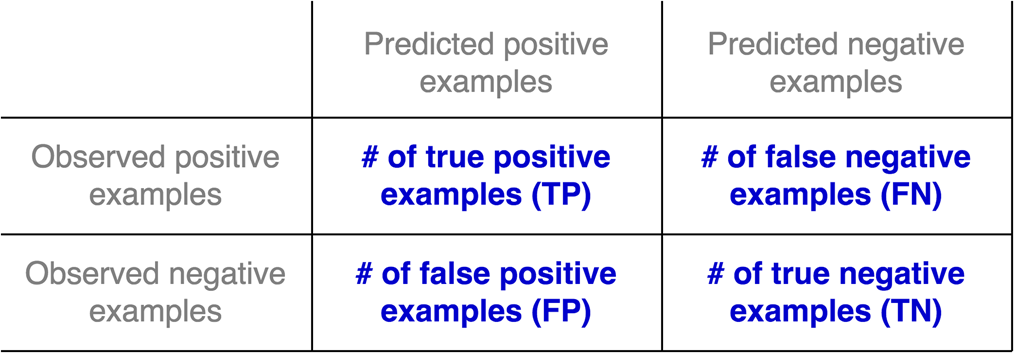
Fig. 3. The confusion matrix. The confusion matrix is typically used for evaluating the performance of machine learning classifiers.
Prediction accuracy (PAC)
Prediction or classification accuracy represents the ratio between the number of correct predictions versus the total number of input samples. Based on the confusion matrix, the PAC is defined as below:
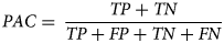 $$PAC = \; \displaystyle{{TP + TN} \over {TP + FP + TN + FN}}$$
While accuracy is widely used in many studies, it doesn't perform well then, the data set is imbalanced and therefore extra caution must be taken when using this metric in isolation.
Precision or positive prediction value
Precision is defined as a function of the total number of TP and FP examples:
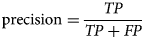 $${\rm precision} = \displaystyle{{TP} \over {TP + FP}}$$
Recall, sensitivity, Hit rate or true positive rate (TPR)
Recall or sensitivity is defined as a function of the total number of TP and FN examples:
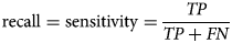 $${\rm recall} = {\rm sensitivity} = \displaystyle{{TP} \over {TP + FN}}$$
In principle, sensitivity measures the proportion of correctly identified positive examples.
Specificity, selectivity or true negative rate (TNR)
Specificity is defined as a function of the total number of TN and FP examples:
 $${\rm specificity} = \displaystyle{{TN} \over {TN + FP}}$$
Specificity measures the proportion of correctly identified negative examples.
F1 score
The F1 score combines precision and recall in a harmonic mean:
 $$F1\; \,{\rm score} = 2 \times \displaystyle{{{\rm precision} \times {\rm recall}} \over {{\rm precision} + {\rm recall}}}$$
Matthews correlation coefficient (MCC)
Introduced in 1975 by Brian Matthews (Matthews, Reference Matthews1975) and regarded by many scientists as the most informative score that connects all four measures in a confusion matrix, the Matthews Correlation Coefficient is typically used in ML to measure the quality of binary classifications and it is particularly useful when there is a significant imbalance in class sizes (data). MCC is calculated according to the following expression:
 $$MCC = \displaystyle{{TP \times TN-FP \times FN} \over {\sqrt {(TP + FP) \times (TP + FN) \times (TN + FP) \times (TN + FN)}}} $$
If any of the denominator terms equals zero, it will be set to 1 and MCC becomes zero, which has been shown to be the correct limiting value for MCC. It returns a value between −1 and 1, where 1 means a perfect prediction, 0 means no better than random and −1 means a total disagreement between predicted and observed values.
Area under the receiver operating characteristic (AUC)
A Receiver Operating Characteristic (ROC) curve is a visual way of describing the tradeoff between sensitivity and specificity (Fig. 4). The closer the curve is to the left-hand and top borders of the plot, the more accurate the method is. The closer the curve is to the main diagonal, the less accurate the method is. AUC is a direct measure of the accuracy of a method. When two or more methods are compared using this approach, the one with the highest AUC value is deemed to be superior. For more information about using the area under the ROC curve please consult (Metz, Reference Metz1978).
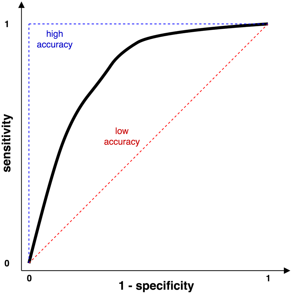
Fig. 4. The Receiver Operating Characteristic (ROC) curve.
Application of ML prediction techniques in animal breeding
Given the known boundaries and limitations of traditional breeding models and techniques, ML approaches have started to slowly but steadily being applied in livestock breeding and traits selection. While their current adoption level in the breeding research community is still low, these advanced methods provide mechanisms to improve regularization by assigning different prior distributions to marker effects and to efficiently select subsets of markers that have better predictive capabilities for specific traits of interest. Below we provide a succinct description of how ML methods are applied in various livestock breeding fields (summarized in Table 1). We grouped the reviewed work in 6 main application domains relevant for animal scientists: health, production, fertility, mortality, nutrition, and breeding.
Table 1. Machine learning methods applied to livestock breeding
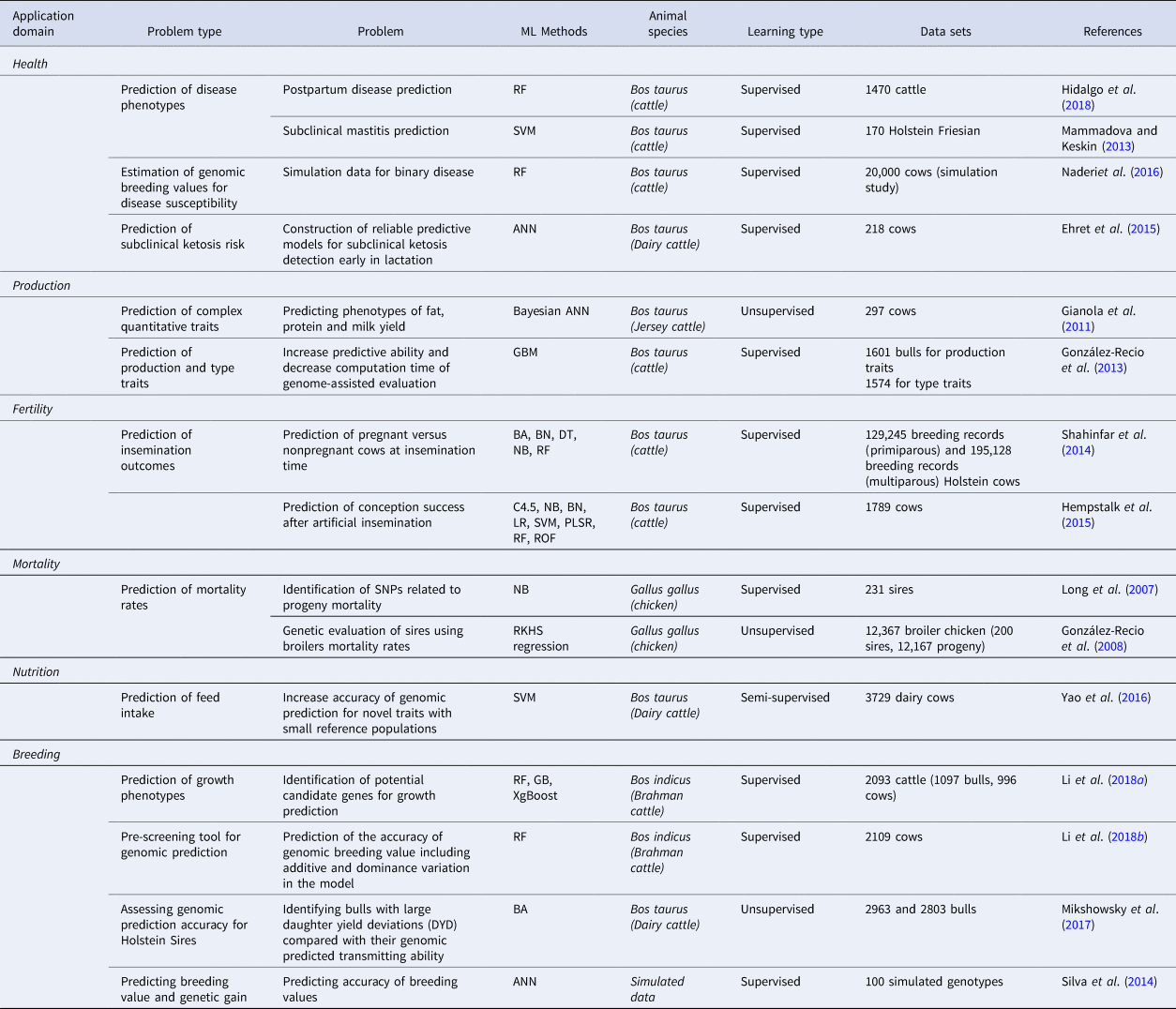
BA, bagging (bootstrap aggregation or ensemble of decision trees); BN, Bayesian networks; C4.5, C4.5 decision trees; DT, decision trees; GB, Gradient Boosting; LR, logistic regression; NB, naïve Bayes; PLSR, partial least squares regression; RB, Random Boosting; RF, Random Forests; RKHS, reproducing kernel Hilbert spaces; ROF, rotation forest; SVM, support vector machines; XgBoost, Extreme Gradient Boosting Method.
Health
Prediction of subclinical ketosis risk
Subclinical ketosis is one of the most important metabolic diseases in high-producing dairy cattle (Collard et al., Reference Collard, Boettcher, Dekkers, Petitclerc and Schaeffer2000). This trait is commonly affected by multiple factors and therefore, constructing a reliable predictive model is challenging. Assessing the applicability of different sources of information in predicting subclinical ketosis in early lactation using ANNs has been performed in German Holstein cattle by Ehret et al. (Reference Ehret, Hochstuhl, Krattenmacher, Tetens, Klein, Gronwald and Thaller2015). In their study, first genomic and metabolic data and the information on milk yield and composition of 218 high-yielding dairy cows during their first 5 weeks of lactation were collected and then the ANN was applied to investigate the ability to predict milk levels of β-hydroxybutyrate (BHB) within and across consecutive weeks postpartum. All animals were genotyped with a 50,000 SNP panel and information on the milk composition data (milk yield, fat and protein percentage) as well as the concentration of milk metabolites, glycerophosphocholine, and phosphocoline, were collected weekly. The concentration of BHB acid in milk was used as target in all prediction models (Ehret et al., Reference Ehret, Hochstuhl, Krattenmacher, Tetens, Klein, Gronwald and Thaller2015). For the prediction analysis, a multilayer feed-forward ANN with a single hidden layer containing five neurons in the hidden layer was designed and a learning rate equal to 0.02 was chosen. Considering the small sample size used in the Ehret et al. (Reference Ehret, Hochstuhl, Krattenmacher, Tetens, Klein, Gronwald and Thaller2015) study, a 5-fold cross validation with 100 individual repetitions (500 independent cross-validations in total) was used to properly assess the predictive ability of the different models within and between consecutive weeks. The predictive ability of each model was calculated using a Pearson correlation (r) between the observed and predicted BHB concentrations averaged over all 500 cross-validation runs (Kohavi and Kohavi, Reference Kohavi and Kohavi1995; Ehret et al., Reference Ehret, Hochstuhl, Krattenmacher, Tetens, Klein, Gronwald and Thaller2015). Their study showed that by considering all implemented models, correlation averages of 0.348, 0.306, 0.369, and 0.256 was obtained for the prediction of subclinical ketosis in weeks 1, 3, 4, and 5 postpartum, respectively. The highest average correlation (0.643) was obtained when milk metabolite and routine milk recording data were combined for prediction on the same day within weeks. A combination of genetic and metabolic predictors did not show a significant increase in the predictive ability of subclinical ketosis, which was explained by the statistical limitations and the complexity of the model when the number of parameters to be estimated increased. Ehret et al. (Reference Ehret, Hochstuhl, Krattenmacher, Tetens, Klein, Gronwald and Thaller2015) suggested that a higher sample size (animals) for ML approaches is required to make SNP-based predictions valuable.
Estimation of genomic breeding values for disease susceptibility
Naderi et al. (Reference Naderi, Yin and König2016) carried out a simulation study to investigate the performance of RF and genomic BLUP (GBLUP) for genomic prediction using binary disease traits based on cow calibration groups. They compared the accuracy of genomic predictions through altering the heritability, number of QTL, marker density, the LD structure of the genotyped population and the incidence of diseased cows in the training population. They also investigated the RF estimates for the effects and locations of the most important SNPs with true QTL (Naderi et al., Reference Naderi, Yin and König2016). Several scenarios were considered where the included genotypes were 10 K (10,005 SNPs) and 50 K (50,025 SNPs) evenly spaced SNPs on 29 chromosomes. The training and testing sets included 20,000 cows (4000 sick and 16,000 healthy with 20% disease incidence) from the last two generations. The number of QTLs was considered 10 (290 QTLs) or 25 (725 QTLs) on each chromosome and the heritabilities of traits were assumed h 2 = 0.10 (low) and h 2 = 0.30 (moderate). The GEBV was estimated using the AI-REML algorithm from the DMU software package (Madsen and Jensen, Reference Madsen and Jensen2013), which allows the specification of a generalized LMM. The RF analysis was applied using the Java package RanFoG (González-Recio and Forni, Reference González-Recio and Forni2011) where thousands of classification trees were constructed through bootstrapping of the data in the training set (Efron and Tibshirani, Reference Efron and Tibshirani1994; Breiman, Reference Breiman2001). RF used on average about two-thirds of the observations and a random subset p of the m SNP (p ~ 2/3 × m). For both GBLUP and RF, PAC was evaluated as the correlations between genomic and true breeding values. Results indicated that for 10 K SNP chip panels and for all percentages of sick cows in the training set, prediction accuracies from GBLUP always outperformed the ones obtained with RF estimations. In the RF method, the prediction was based on a random subsample of SNs. Therefore, with low-density marker panels, the QTL signal of a distant SNP might not be captured due to insufficient sampling of that SNP. The application of the 50 K SNP panel for analyzing binary data resulted in a more accurate ranking of the individuals with the RF method compared with GBLUP. In addition, RF could distinguish more precisely between healthy and affected individuals in most allocating schemes. The highest PAC was obtained for a disease incidence of 0.20 in the training sets and was equal to 0.53 for RF and 0.51 for GBLUP (using a 50k SNP panel, a heritability of 0.30 and 725 QTLs). Naderi et al. (Reference Naderi, Yin and König2016) concluded that in general, prediction accuracies are higher when using the GBLUP methodology and the decrease in heritability and number of QTLs was associated with a decrease in prediction accuracies for all the scenarios where it was more pronounced for the RF method. The RF method performed better than GBLUP only when the highest heritability, the denser marker panel and the largest number of QTLs were used for the analyses. Furthermore, the RF method could successfully identify important SNPs in close proximity to a QTL or a candidate gene.
Prediction of disease phenotypes
Hidalgo et al. (Reference Hidalgo, Zouari, Knijn and van der Beek2018) used the RFML approach to predict the probability of occurrence of postpartum disease (60 days) in 1470 dairy cattle based on prepartum data (250 days). Data were collected from six Dutch farms encompassing a total of 59,590 records split into 70–30% training-testing data sets and 46 features were used to train their algorithm. They reported an AUC score of 0.77 for data that did not include breeding values as training features. When such features were included in the training of the model, the AUC increased to 0.81, showing an improved performance of the RF approach on this dataset (Hidalgo et al., Reference Hidalgo, Zouari, Knijn and van der Beek2018).
Mammadova and Keskin (Reference Mammadova and Keskin2013) used SVMs to ascertain the presence of subclinical and clinical mastitis in dairy cattle. They used 346 (61 mastitis cases) measurements of milk yield, electrical conductivity, average milking duration and somatic cell count collected from February 2010 to April 2011 for 170 Holstein Friesian dairy cows. They reported high sensitivity (89%) and specificity (92%) values for the SVM approach in comparison with a traditional binary logistic regression model, whose sensitivity and specificity values were 75 and 79%, respectively (Mammadova and Keskin, Reference Mammadova and Keskin2013).
Production
ANNs have been introduced as a new method that can be employed in genetic breeding for selection purposes and decision-making processes in various fields of animal and plant sciences (Gianola et al., Reference Gianola, Okut, Weigel and Rosa2011; Nascimento et al., Reference Nascimento, Alexandre Peternelli, Damião Cruz, Carolina Campana Nascimento, de Paula Ferreira, Lopes Bhering and Césio Salgado2013). These learning machines (ANN) can act as universal approximators of complex functions (Alados et al., Reference Alados, Mellado, Ramos and Alados-Arboledas2004). Additionally, these learning approaches can capture non-linear relationships between predictors and responses and learn about functional forms in an adaptive manner (Gianola et al., Reference Gianola, Okut, Weigel and Rosa2011). Gianola et al. (Reference Gianola, Okut, Weigel and Rosa2011) investigated various Bayesian ANN architectures to predict milk, fat, and protein yield in Jersey. A feed-forward neural network with three layers and five neurons in the hidden layer was considered. Predictor variables for Jersey cows were derived from pedigree and 35,798 SNPs from 297 cows. The results showed that the predictive correlation in Jerseys was clearly larger for non-linear ANN, with correlation coefficients between 0.08 and 0.54, while the linear models had correlation coefficients between 0.02 and 0.44. Furthermore, the ability to predict fat, milk, and protein yield was low when using pedigree information and improved when SNP information was employed in the prediction analysis as measured by the predictive correlations (Gianola et al., Reference Gianola, Okut, Weigel and Rosa2011). In summary, Gianola et al. (Reference Gianola, Okut, Weigel and Rosa2011) concluded that the predictive ability seemed to be enhanced by the use of Bayesian neural networks, however, due to small sample sizes, further analysis on different species, traits and environment was recommended.
González-Recio et al. (Reference González-Recio, Jiménez-Montero and Alenda2013) proposed a modified version of the gradient boosting (GB) algorithm called random boosting (RB), which increases the predictive ability and significantly decreases the computation time of genome-assisted evaluation for large data sets when compared to the original GB algorithm. They applied their technique on a data set comprising 1797 genotyped bulls including 39,714 SNPs and using four yield traits (milk yield, fat yield, protein yield, fat percentage) and one type trait (udder depth) as dependent variables. They used sires born before 2005 as a training set and younger sires as a testing set to evaluate the predictive ability of their algorithm on yet-to-be-observed phenotypes. The results of the RB method produced comparable accuracy with the GB algorithm whereas it ran in 1% of the time needed by GB to produce the same results (González-Recio et al., Reference González-Recio, Jiménez-Montero and Alenda2013). The Pearson correlation between predicted and observed responses for GB and RB ranged between 0.43 and 0.77 for different values of percentages of SNP sampled at each iteration and 3 smoothing parameters (0.1, 0.2, and 0.3).
Fertility
Shahinfar et al. (Reference Shahinfar, Page, Guenther, Cabrera, Fricke and Weigel2014) compared five ML techniques (BA, BN, DT, NB, RF) to predict insemination outcomes in Holstein cows. They used data collected over a 10-year period (2000–2010) from 26 Wisconsin dairy farms that included 129,245 breeding records from primiparous Holstein cows and 195,128 breeding records from multiparous Holstein cows. Each breeding information record included production data, EBV, health events, and reproduction information. While all five algorithms were effective at predicting pregnant versus nonpregnant cows, RF outperformed the other four in terms of classification accuracy (72.3% for primiparous cows and 73.6% for multiparous cows) and area under the ROC curve (75.6% for primiparous cows and 73.6% for multiparous cows). They identified five factors to be the most informative features for predicting insemination outcome: the mean within-herd conception rate in the past 3 months, herd-year-month of breeding, days in milk at breeding, number of inseminations in the current lactation, and stage of lactation when the breeding occurred (Shahinfar et al., Reference Shahinfar, Page, Guenther, Cabrera, Fricke and Weigel2014).
Hempstalk et al. (Reference Hempstalk, McParland and Berry2015) used herd- and cow-level factors such as parity number, animal breed, PTA (measure of genetic merit), calving interval, milk production, live weight, longevity, the Irish Economic Breeding Index and mid-infrared (MIR) spectral data (1060 points) to predict the likelihood of conception success to a given insemination. They also investigated the usefulness of adding the MIR data to augment the accuracy of the prediction models. Their study used a dataset comprising 4341 insemination records with conception outcome information from 2874 lactations on 1789 cows (61.1% Holstein-Friesian, 12% Jersey, 5.8% Norwegian Red, and 21.1% crossbred animals) from seven research herds for a 5-year period between 2009 and 2014. They tested eight ML algorithms including C4.5 DT, NB, Bayesian network (BN), logistic regression, SVM, PSLR, RF, and ROF. The performance of the 8 algorithms with respect to the area under the ROC curve was deemed to be fair with values between 0.487 and 0.675, the overall best performing algorithm being the logistic regression, followed closely by ROF and SVM. These results were expected given the presence of many factors that are not known a priori, which significantly contribute to the prediction outcome, such as herd-year-season of insemination, insemination technician capability, and mate fertility. They also concluded that the inclusion of MIR data in the models did not improve the accuracy of prediction for this particular classification problem (Hempstalk et al., Reference Hempstalk, McParland and Berry2015).
Mortality
Long et al. (Reference Long, Gianola, Rosa, Weigel and Avendaño2007) explored ML methods for identifying SNPs associated with chick mortality in broilers. They used mortality records for early age (0–14 days) progenies of 231 randomly chosen sires, which were part of an elite broiler chicken line raised in high and low hygiene environments (Long et al., Reference Long, Gianola, Rosa, Weigel and Avendaño2007). The ML approach applied discretization of continuous mortality rates of sire families into two classes and consisted of a 2-step SNP discovery process. The first step was based on dimensionality reduction and used information gain to reduce the initial number of SNPs to a more manageable subset. The second step used a Bayes classifier to optimize the performance of the selected SNPs. Results suggested that the SNP selection method, coupled with sample partition and subset evaluation procedures, provided a useful tool for finding 17 important SNPs relevant to chick mortality in broilers.
González-Recio et al. (Reference González-Recio, Gianola, Long, Weigel, Rosa and Avendaño2008) compared five regression approaches (E-BLUP, F∞-metric model, kernel regression, reproducing kernel Hilbert spaces (RKHS) regression, Bayesian regression) with a standard procedure for genetic evaluation (E-BLUP) of sires using mortality rates in broilers as a response variable and SNP information. They used mortality records on 12,167 progenies of 200 sires and two sets of SNPs: one set of 24 SNPs potentially associated with mortality rates for three of the methods used for genomic assisted evaluations and a set of 1000 SNPs covering the whole genome for the Bayesian regression (González-Recio et al., Reference González-Recio, Gianola, Long, Weigel, Rosa and Avendaño2008). The RKHS regression approach consistently outperformed the other methods with an accuracy gain between 25% and 125%. The global Pearson correlation coefficient between predicted and actual values of the progeny average of each sire for late mortality was 0.20 for RKHS and significantly lower for E-BLUP (0.10), F∞-metric model (0.08), kernel regression (0.14) and Bayesian regression (0.16).
Nutrition
Accuracy of genomic prediction for novel traits is often hampered by the limited size of the reference population and the number of available phenotypes. ML tools have the potential to address this challenge through a semi-supervised learning method (Zhu and Goldberg, Reference Zhu and Goldberg2009). Yao et al. (Reference Yao, Zhu and Weigel2016) investigated a semi-supervised learning method called the self-training model wrapped around a SVM algorithm and applied this method to genomic prediction of residual feed intake (RFI) in dairy cattle. In the Yao et al. (Reference Yao, Zhu and Weigel2016) study, a total number of 57,491 SNPs were available for 3792 dairy cows. From this number of animals, 792 cows were measured for RFI phenotype and 3000 cows were without a measured RFI phenotype. The SVM model was trained using the 792 animals with measured phenotypes and then the result was used to generate a self-trained phenotype for 3000 animals without phenotype. Eventually, the SVM model was re-trained using data from 3792 animals with measured and self-trained RFI phenotypes. Their study indicated that for a given training set of animals with measured phenotype, improvements in PAC (measured as the correlation associated with semi-supervised learning) increased as the number of additional animals with self-trained phenotypes increased in the training set. The highest correlation was 5.9% when the ratio of animals with self-trained phenotype models to the animals with actual measured phenotypes was 2.5. The authors suggested that the semi-supervised learning method may be a helpful tool to enhance the accuracy of genomic prediction for novel traits (that are difficult or expensive to measure) with small reference population size. However, further research is recommended.
Breeding
Prediction of genomic predicted transmitted ability
Bootstrap aggregation sampling (bagging) is a resampling method that can increase the accuracy of predictions at the time that sampling from the training set leads to large variance in the predictor (Breiman, Reference Breiman2001). Mikshowsky et al. (Reference Mikshowsky, Gianola and Weigel2017) applied a variation of the bootstrap aggregation (bagging) in GBLUP (BGBLUP) to predict genomic predicted transmitting ability (GPTA) and reliability values of 2963, 2963 and 2803 young Holstein bulls for protein yield, somatic cell score and daughter pregnancy rate (DPR), respectively. For each trait, 50 bootstrap samples were randomly selected from a reference population as recommended by Gianola et al. (Reference Gianola, Weigel, Krämer, Stella and Schön2014) and GBLUP was used to compute the genomic predictions for each trait in the testing set. The results found bootstrap standard deviation (SD) of GBLUP predictions to be statistically significant for identifying bulls with future daughters having significantly better performance (deviate significantly from early GPTA) for protein and daughter pregnancy rate. Furthermore, bulls with more close relatives in the training and testing population showed less variation in their bootstrap predictions. Bootstrap samples containing the sire had a smaller range of bootstrap SD, which confirmed that the presence of sires in the reference population helps to stabilize predictions. The authors observed that the maximum BGBLUP correlation (0.665 for proteins, 0.584 for SCS, 0.499 for DPR) for any sample was always below that of the GBLUP correlation (0.690 for proteins, 0.609 for SCS, 0.557 for DPR) from the full reference population, and the minimum BGBLUP mean-squared error (MSE) for any individual sample was always larger than that of the GBLUP MSE. Mikshowsky et al. (Reference Mikshowsky, Gianola and Weigel2017) suggested that bootstrap prediction reliability is an effective method to construct useful diagnostic tools for assessment of genomic prediction systems or to evaluate the composition of a genomic reference population.
Genomic breeding values for growth
Li et al. (Reference Li, Zhang, Wang, George, Reverter and Li2018a) used three ML approaches (RF, GBM, XgBoost) and 38,082 SNP markers and live body weight phenotypes from 2093 Brahman cattle (1097 bulls as a discovery population and 996 cows as a validation population) to identify subsets of SNPs to construct genomic relationship matrices (GRMs) for the estimation of genomic breeding values (GEBVs). Of all three methods, GBM had the best performance and was then followed by RF and XgBoost. The average PAC values across 400, 1000, and 3000 SNPs were 0.38 for RF, 0.42 for GBM, and 0.26 for XgBoost, when applied to identify potential candidate genes for the growth trait (Li et al., Reference Li, Zhang, Wang, George, Reverter and Li2018a). When the authors used all SNPs with positive variable importance values, they achieved similar PAC (0.42 for RF, 0.42 for GBM and 0.39 for XgBoost) when compared with the 0.43 overall accuracy from the whole SNP panel. The results suggest that when it comes to the genomic prediction of breeding values, more SNPs in a model do not necessarily translate to a better accuracy. The authors concluded that the subsets of SNPs (400, 1,000, and 3000) selected by the RF and GBM methods significantly outperformed those SNPs evenly spaced across the genome. Nevertheless, the superiority of the GBM performance comes at the expense of longer computational time when compared to RF and other methods.
Prediction of breeding values and genetic gains
In another study carried out by Silva et al. (Reference Silva, Tomaz, Sant'Anna, Nascimento, Bhering and Cruz2014), the ability of ANN for the prediction of breeding values was evaluated using simulated data and other relevant statistics as well as the mean phenotypic value. In the simulation scenarios, two sets of simulated characteristics were considered with heritabilities between 40 and 70%. They employed a randomized block design with 100 genotypes and six blocks, and the mean values and coefficient variation were assumed to be 100 and 15%, respectively. The data expansion process was performed using the integration module in the computer application GENES. The expansion process applied statistical methods that allowed the preservation of traits such as the mean, variance and covariance among information of the genotypes, which were considered pairs of blocks from the original data (Silva et al., Reference Silva, Tomaz, Sant'Anna, Nascimento, Bhering and Cruz2014). Feed-forward back propagation multilayer perceptron networks were created in Matlab using the integration module in the computer application of GENES. The network architecture consisting of three hidden layers in the training algorithm trainlm and activation functions transig or logsig was used. The number of neurons were varying from one to seven and a maximum of 2000 iterations was considered. The result of this study showed that the estimates of prediction accuracies by the ANN, considering of 120 validation experiments, were on average 1% (heritability 40%) and 0.5% (with heritability of 70%) higher compared with the traditional methodologies (based on least squares estimates). Therefore, Silva et al. (Reference Silva, Tomaz, Sant'Anna, Nascimento, Bhering and Cruz2014) concluded that ANNs have great potential for the use as an alternative model in genotypic selection to predict genetic values.
Genomic prediction of body weight
In a study carried out by Li et al. (Reference Li, Raidan, Li, Vitezica and Reverter2018b) a RF method was used as a prescreening tool to identify subsets of SNPs for genomic prediction of total genetic values of yearling weight in beef cattle. The purpose of their study was to investigate the effect of unknown non-additive factors (e.g. epistatic effects of SNPs) in the PAC of total genetic values using ML methods. The dataset consisted of 651,253 genotyped SNPs from 2109 Brahman beef cattle and the phenotypes were measured on the animals and adjusted for fixed effects (contemporary group, age and the average of heterozygosity) of all SNPs for each animal. The residuals from the analysis of variance (linear model) were then used as the phenotype for the evaluation of RF. The details of the RF method used in their study was explained in Breiman (Reference Breiman2001) where training and validation procedures were used to build DT with a subset of animals and SNPs. They used a SNP variable important value measured as the percentage of increased MSE after a SNP is randomly permuted in a new sample (Breiman, Reference Breiman2001). Additive and dominance genomic relationship matrices, GRM and DRM, respectively (Vitezica et al., Reference Vitezica, Varona and Legarra2013) were constructed for a subset of 500, 1,000, 5,000, 10,000, and 50,000 SNPs and were included in the model to predict the genomic value. A 5-fold cross validation approach was used to compute the accuracy. The results of their study using the RF method showed that including the dominance variation in the genomic model neither had impact on the estimate of heritability nor on the additive variance and accuracy of prediction. However, RF could identify subsets of SNPs that had significantly higher genomic PAC (0.45–0.60) than using all SNPs (0.44). Taking all these results together, Li et al. (Reference Li, Raidan, Li, Vitezica and Reverter2018b) suggested that the RF method has the potential to be used as a pre-screening tool for reduction of high dimensionality of the large genomic data and identification of the subset of useful SNPs for genomic prediction of breeding values.
Summary of results
A summary of the results obtained with ML techniques applied to the 6 animal science domains of activity is summarized in Table 2. As it can be easily observed, the metrics used to evaluate and compare the results obtained with various traditional and ML methods include only a limited subset of evaluation metrics traditionally used in the ML field and listed in a previous section in this manuscript. Some of the used evaluation methods, such as PAC and correctly classified instances (CCI) are either very sensitive to the distribution of the data or capture only the positive examples correctly predicted by the ML approaches, thus making the overall interpretation and comparison of the results problematic.
Table 2. Comparison of ML methods applied in different areas of animal science and their corresponding evaluation methodologies
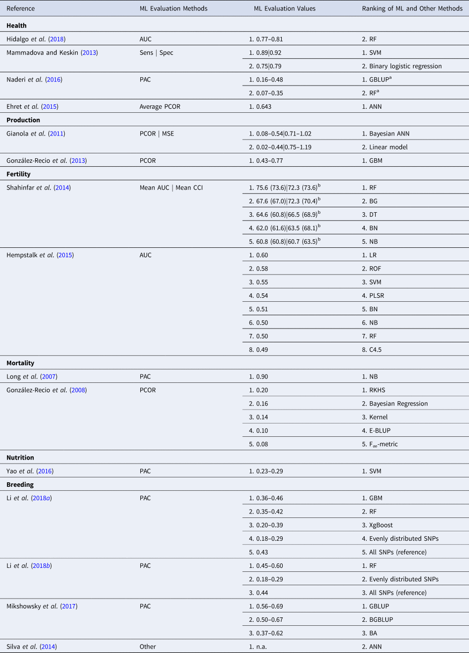
AUC, area under the ROC curve; Sens, sensitivity; Spec, specificity; PAC, prediction accuracy; PCOR, Pearson product moment correlation coefficient; CCI, correctly classified instances; MSE, mean-squared error; other, other evaluation method not typically used in the ML field; n.a., not applicable.
a Order of ranked methods reversed for high heritability.
b Primiparous (Multiparous) values.
It can be also observed, that regardless of the application domain, there is no clear ML method winner. While some methods such as RF, GBMs), ANNs and SVM tend to outperform other ML methods or traditional approaches (Gianola et al., Reference Gianola, Okut, Weigel and Rosa2011; Shahinfar et al., Reference Shahinfar, Page, Guenther, Cabrera, Fricke and Weigel2014; Li et al., Reference Li, Zhang, Wang, George, Reverter and Li2018a, Reference Li, Raidan, Li, Vitezica and Reverter2018b), there are instances where traditional approaches such as linear regression, GBLUP and BGBLUP outperform the ML ones (Hempstalk et al., Reference Hempstalk, McParland and Berry2015; Naderi et al., Reference Naderi, Yin and König2016; Mikshowsky et al., Reference Mikshowsky, Gianola and Weigel2017). This suggests that it is not always the case that ML methods apply well to all problems and their successful performance strongly depends on many factors such as the nature of the problem (e.g. classification, clustering, dimensionality reduction, regression), choosing a correct and direct problem encoding (e.g. decision versus prediction), the quality of the data (e.g. noisy, highly redundant, missing values) and various data types (e.g. discrete, continuous, categorical, numeric).
In some cases, the evaluation results of various ML and traditional methods summarized on column 3 from Table 2 are low compared with similar studies performed in different areas of research. For example, Naderi et al. (Reference Naderi, Yin and König2016) obtained prediction accuracies <0.55 for both GBLUP and RF, which indicate low-performance classifiers. Nevertheless, the low-density SNP-based datasets and simulated data used in their study most probably contributed to the low accuracy values.
In a handful of studies, Pearson correlations are applied to measure the agreement between predicted and observed results. While this approach is a valid statistical measure to estimate linear correlations and can be potentially applied in the study, the obtained correlation coefficients were, for example, lower than 0.2 for all the five methods reported by González-Recio et al.(Reference González-Recio, Gianola, Long, Weigel, Rosa and Avendaño2008). In a typical study, this might suggest no correlation among results, but given the very low genome coverage of SNP data (only 1000 SNPs for the whole genome) and the possibility that not all mortality events might be related to the 24 SNPs potentially associated with mortality, the results are not surprising.
In summary, it is recommended that the employment of ML methods applied in animal science breeding should be accompanied by the adoption and careful selection of appropriate and homogeneous metrics for estimating the quality of predictive results. It is also desirable that more than one ML method is selected for a study and the results must be compared against each other and against results obtained with more traditional approaches as it was already reported previously (Mammadova and Keskin, Reference Mammadova and Keskin2013; Hempstalk et al., Reference Hempstalk, McParland and Berry2015; Naderi et al., Reference Naderi, Yin and König2016).
Conclusions
In summary, the work reviewed in this article showcases a methodological transition in livestock breeding, from traditional prediction strategies such as single-step GBLUP, MAS and GWAS to more advanced ML approaches including ANNs, DL, BN, and various ensemble methods. While the adoption of the more advanced methods happened much faster in the human health and plant breeding sectors, it is still in its infancy in the livestock breeding sector and more work must be done on both, research and applied fronts, to create more convincing and easier to adopt strategies for the livestock breeding community of practice. One potential first step to achieve this goal would be to merge traditional and novel approaches into a hybrid solution that would offer a smoother transition to newer and more powerful predictive systems that are easier to adopt by practitioners and researchers alike. We also believe that the adoption of ML methods to be applied in animal breeding research must be accompanied by the adoption of corresponding and, when necessary, introduction of new evaluation metrics that better capture the quality of the results. Thus, innovative methods and strategies are needed to handle the deluge of data and facilitate a smoother transition, which should be the focus of future research efforts in the near future.
Acknowledgments
The work conducted in the Tulpan Laboratory is supported by the Food from Thought research program at University of Guelph (grant no. 499063). We would like to thank the editors and anonymous reviewers for their support and suggestions to improve this manuscript.


