


Introduction
The East Antarctic ice sheet is traditionally considered a stable feature characterized by slow-moving interior ice with drainage through ice shelves across a grounding line and by a few faster-moving outlet glaciers. This view is now challenged by new evidence coming from balance velocities (the depth-averaged velocity required to keep the ice sheet in steady state for a given net surface mass accumulation) obtained from radar altimetry and radio-echo sounding, as well as surface velocities obtained from interferometric synthetic aperture radar (Reference Bamber, Vaughan and JoughinBamber and others, 2000). Complex ice flow (a combination of ice flow due to internal deformation and basal motion) was already observed within the West Antarctic and Greenland ice sheets (Reference JoughinJoughin and others, 1999, Reference Joughin, Fahnestock, MacAyeal, Bamber and Gogineni2001), and recent studies confirm a similar complexity within the East Antarctic ice mass (Reference PattynPattyn and Naruse, 2003; Reference Rippin, Bamber, Siegert, Vaughan and CorrRippin and others, 2003). Balance-velocity maps reveal a complex network of enhanced-flow tributaries penetrating several hundred kilometers into the ice-sheet interior (Reference Bamber, Vaughan and JoughinBamber and others, 2000; Reference Testut, Hurd, Coleman, Rémy and LegrésyTestut and others, 2003). In this paper, we investigate such features observed in Dronning Maud Land, East Antarctica, and try to disentangle the mechanisms that control their existence and behavior with a three-dimensional thermomechanically coupled ice-sheet model including higher-order stress gradients, coupled to a steady-state model of basal water flow.
Data
The Ragnhild glaciers are three, as yet nameless, ice-flow features situated between the Sør Rondane and Yamato Mountains in east Dronning Maud Land. They are clearly identified as enhanced ice-flow features in maps of balance fluxes of the Antarctic ice sheet. The largest feature, here referred to as west Ragnhild glacier (WRG), penetrates almost 400 km inland (Fig. 1). RADARSAT imagery reveals distinct flowlines along the ice surface, but they are less apparent than those of other large ice streams and outlet glaciers of East Antarctica. A comparison between 1937 Norwegian maps and 1960 Belgian maps permitted Reference Nishio, Ishikawa, Ohmae, Takahashi and KatsushimaNishio and others (1984) to determine the horizontal movement of the ice-shelf front along the Princess Ragnhild Coast. Derwael Ice Rise is situated directly in front of WRG, so most of the ice flow is diverted around this buttressing feature. The maximum flow speed occurs at the western side (350ma–1), while flow velocities to the east of Derwael Ice Rise are somewhat lower. A comparison between 1965 Belgian maps and RADARSAT imagery (Reference JezekJezek and RAMP Product Team, 2002) shows an acceleration in the west and a deceleration towards the east along the Princess Ragnhild Coast (Table 1). The latter might indicate an eventual stoppage of the glaciers in the center and the east of the catchment area. Ice-flow measurements in the interior of the drainage basin are sparser, but clearly mark a velocity of 100ma–1 on WRG between the Sør Rondane and Belgica Mountains (Reference Takahashi, Naruse, Nishio and WatanabeTakahashi and others, 2003). This is relatively fast for typical ice-sheet flow so far inland. According to Reference Bindschadler, Bamber, Anandakrishnan, Alley and BindschadlerBindschadler and others (2001), 100 ma–1 can be considered the lower limit of ice-stream flow in Antarctica. Ice speed on central Ragnhild glacier (CRG) is distinctly lower.

Fig. 1. Satellite image map based on RADARSAT–RAMP (RADAR-SAT-1 Antarctic Mapping Project) imagery (Reference JezekJezek and RAMP Product Team, 2002). The thick black line delimits the modeled drainage basin (only part of the catchment is shown). Measured velocities (arrows) are taken from Reference Takahashi, Naruse, Nishio and WatanabeTakahashi and others (2003). Calculated balance fluxes are shown in gray-shaded contours (unlabeled); surface topography (m a.s.l.) in white contours.
Table 1. Velocity estimates (m a–1) of the ice shelf along the Princess Ragnhild Coast, 1937–60 (Reference Nishio, Ishikawa, Ohmae, Takahashi and KatsushimaNishio and others, 1984) and 1965–97 (this study). Markers correspond to positions in Figure 1

If these stream features exist, they are to a certain extent topographically controlled. Airborne radar surveys reveal that the coastal mountain blocks are interspersed by large subglacial valleys with their floors lying below sea level (Reference Nishio, Uratsuka, Ohmae and HigashiNishio and others, 1995). These ice-thickness measurements, included in the BEDMAP database (Reference Liu, Jezek and LiLiu and others, 1999; Reference Lythe and VaughanLythe and others, 2001), form the major source material for the numerical experiments carried out below. For the prognostic experiments, surface mass balance was taken from Reference Vaughan, Bamber, Giovinetto, Russell and CooperVaughan and others (1999).
Model Description
The model approach is based on continuum thermodynamic modelling, and encompasses balance laws of mass, momentum and energy, extended with a constitutive equation. A complete description of the model is given in Reference Pattyn and NarusePattyn (2003).
The force-balance equations are
where σij are the shear stress and σ′ ii the deviatoric normal stress components, ρ i is the ice density, g is the gravitational constant and z s is the surface elevation of the ice mass. The constitutive equation governing the creep of polycrystalline ice and relating the deviatoric stresses to the strain rates is taken as a Glen-type flow law with exponent n = 3 (Reference PatersonPaterson, 1994):
where ɛ is the second invariant of the strain-rate tensor and η is the effective viscosity. The flow-law rate factor is a function of temperature θ (θ * is the temperature corrected for the dependence on pressure melting) and obeys an Arrhenius relationship. The temperature distribution reflects conduction, horizontal and vertical advection, and internal friction due to deformational heating:
where c p and k i are heat capacity and thermal conductivity of the ice, respectively, vi are the velocity components, and σ is the second invariant of the stress tensor.
Instead of modelling the whole Antarctic ice sheet, we limit the model domain to a regional catchment area between the Dome Fuji ice divide and the Princess Ragnhild Coast (Fig. 1). Boundary conditions on the model are a fixed ice thickness at the grounding line and a zero surface slope across the ice divide. Grounding-line motion and ice-shelf dynamics were not included, as this study focuses on the inland part of the ice sheet and the ice stream. To create the input files, the BEDMAP data were resampled to a grid of 10 by 10 km, leading to a model domain of 86 by 86 gridpoints in the horizontal, and 41 layers in the vertical.
Subglacial water and basal sliding
In the model, basal hydrology is represented in terms of the subglacial water flux, which is a function of the basal melt rate. A continuity equation for basal water flow is written as
where w is the thickness of the water layer (m), vw the vertically integrated velocity of water in the layer (ma–1) and ṁb the basal melt rate (ma–1). If we consider steady-state conditions, the basal melt rate must balance the water-flux divergence, or ![]() Basal melting occurs when the ice base reaches the pressure-melting point, and is defined as
Basal melting occurs when the ice base reaches the pressure-melting point, and is defined as
where L is the latent-heat flux, G is the geothermal heat flux, taken as 54.6 mWm–2 (Reference HuybrechtsHuybrechts, 2002), v
b is the basal ice velocity, τ
b the basal drag and θ
b the basal ice temperature. Subglacial water tends to move in the direction of decreasing hydraulic potential ϕ (Reference ShreveShreve, 1972). If we assume that basal water pressure is equal to the overlying ice pressure, the hydraulic potential gradient (or water-pressure gradient) is written as ![]() where ρ
w is the water density and z
b is the lower surface elevation of the ice mass. The steady-state basal water flux
where ρ
w is the water density and z
b is the lower surface elevation of the ice mass. The steady-state basal water flux ![]() is obtained by integrating the basal melt rate m _ over the whole drainage basin, starting at the hydraulic head in the direction of the hydraulic potential gradient ▽ϕ. This is done with the computer scheme for balance-flux distribution of ice sheets described in detail by Reference Budd and WarnerBudd and Warner (1996).
is obtained by integrating the basal melt rate m _ over the whole drainage basin, starting at the hydraulic head in the direction of the hydraulic potential gradient ▽ϕ. This is done with the computer scheme for balance-flux distribution of ice sheets described in detail by Reference Budd and WarnerBudd and Warner (1996).
In large-scale ice-sheet modelling, basal sliding is often taken as being proportional to the basal drag (or driving stress) and inversely proportional to the effective pressure, which is defined as the ice overburden pressure minus the basal water pressure. Reference WeertmanWeertman (1964) relates basal sliding velocity to the driving stress and a roughness factor. The presence of a thin water film underneath an ice sheet will reduce friction and thus bed roughness, hence facilitating basal sliding. In that sense, it is possible to involve basal water-layer thickness as inversely proportional to roughness (Reference Johnson and FastookJohnson and Fastook, 2002). However, water-layer thickness can only be determined if the subglacial water velocity is known. For the sake of simplicity, we assume water velocity constant over the whole drainage basin, so that the subglacial water flux ψw can be inversely related to bed roughness. Although we are aware that in some limit cases, such as a subglacial lake where vw = 0 but the ice velocity across the lake differs from zero, the above relation breaks down, the model results show that ψw generally increases towards the grounding line. As such, we obtain a sliding law, in its most simple form (linear), written as
where A b is a sliding constant and θ pmp is the pressure-melting temperature. The exponential term in Equation (7) allows for basal sliding at subfreezing temperatures over a range of γ = 1 K (Reference Hindmarsh and Le MeurHindmarsh and Le Meur, 2001). Since basal sliding vb also appears in the determination for the
basal melt rate (Equation (6)), Equation (7) is solved iteratively within each time-step. Basal sliding due to subglacial meltwater is likely to occur in the Ragnhild catchment, as evidence of subglacial water flow is found in deglaciated areas in the coastal part of the adjacent drainage basin (Reference Sawagaki and HirakawaSawagaki and Hirakawa 1997).
Standard Experiments
A first series of experiments are diagnostic in nature, i.e. the velocity, stress and temperature fields were calculated by keeping the glacier geometry (ice thickness) fixed. Four experiments were carried out: an isothermal experiment DI where the flow parameter A(θ *) was kept constant at 2×10–17 Pa–n a–1, a model run where the temperature field was coupled to the velocity (DC) and two model runs where basal sliding was included (DIS and DCS). In the thermocoupled experiments (DC and DCS) the temperature-dependent flow parameter was determined as

where a = 1.14 × 10⁻⁵ Pa–n a–1 and Q = 60 kJ mol–1 for θ * < 263.15 K, a = 5.47 × 10¹⁰ Pa –n a–1 and Q = 139 kJ mol–1 for θ * ≥ 263.15 K. The enhancement factor was taken as m = 2, so that modeled and observed velocities are in agreement in experiment DC. The sliding rate factor A b was set to 1.3×10⁻³ Pa–1 m so that modeled velocities agree with observations in experiment DIS. The same parameters were used for experiment DCS. For the thermocoupled experiments, the temperature field was each time run to steady state.
Figure 2 displays the predicted velocity according to the DI and DCS experiments. The isothermal ice-sheet model is not capable of explaining the observed surface velocities nor the pronounced channeling as seen from balance-flux estimates. Introducing thermomechanical coupling and/or basal sliding based on the subglacial water model results in a channeled flow pattern of enhanced ice flow. As seen from Figure 3, sliding and/or coupling result in a similar pattern of ice flow. This striking coincidence becomes clear when comparing the basal water flow with the basal temperature pattern. We therefore calculated the potential basal water flow by assuming that the whole ice sheet in the Ragnhild drainage basin reached the pressure-melting point at the base, with a constant basal melt rate of 1 mma–1. The result of this exercise is shown in Figure 4a and demonstrates that the basal water flow is concentrated in the topographic lows, hence forming an elongated pattern penetrating far inland for the major ice streams in the area. The basal temperature pattern is quite similar, showing the temperature at pressure-melting point for the same channels (Fig. 4b, experiment DC). Introducing basal sliding or temperature coupling leads to a similar pattern in ice flow, with comparable velocities. Cumulating these effects does not alter this pattern nor the magnitude of the surface velocity, although basal sliding is relatively important. The reason for this convergence lies in a negative feedback where increased basal sliding increases the advection of colder ice from above and reduces the amount of vertical shear, hence reducing the thickness of the highly deforming basal ice layer that is at pressure-melting point.

Fig. 2. Predicted surface velocity (m a–1) according to the diagnostic isothermal experiment (DI) and the thermocoupled experiment with basal sliding (DCS).

Fig. 3. Predicted surface velocity (m a–1) according to the four diagnostic experiments DI (small dots), DC (large dots), DIS (thin line) and DCS (thick line).

Fig. 4. (a) Predicted basal water flux (m2 a–1) for a uniform basal melt rate of 1 mma–1. (b) Predicted basal temperature corrected for pressure melting (°C) for the DC experiment.
A second series of experiments consists in running the model in prognostic mode, i.e. by allowing the ice thickness to react to the calculated velocity and temperature distribution and running the model to steady state. Four similar experiments were carried out, one isothermal experiment (PI), one thermocoupled experiment (PC) and two with the addition of basal sliding (PIS and PCS). Similar to the diagnostic experiments, the pattern of channeled flow is only revealed with basal sliding and/or thermomechanical coupling (Fig. 5). Even more apparent is the signature of CRG in addition to WRG. East Ragnhild glacier remains absent as a discernible feature in the simulation (cf. Fig. 1). The velocity fields from the prognostic experiments are more channelized and reach further inland than the velocity fields from the diagnostic experiments.
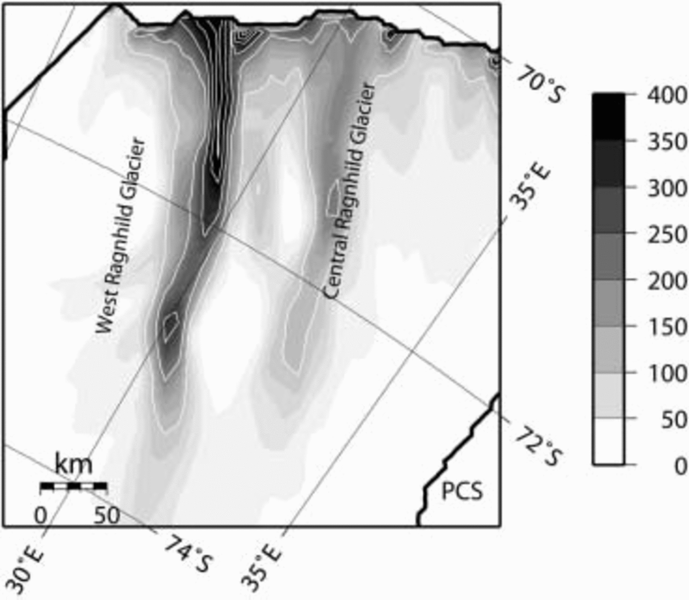
Fig. 5. Predicted surface velocity (m a–1) according to the prognostic thermocoupled experiment with basal sliding (PCS).
Sensitivity of the Ragnhild Glaciers
The effects of basal sliding on the dynamic behavior of the model are assessed in a series of four experiments in which the value of parameter A b in Equation (7) is gradually increased, i.e. A b = 1.3, 2.0, 3.3 and 5.0×10⁻³ Pa–1 m–1. All experiments start from the PCS experiment, and are run to a steady state. In each of the experiments a final time-independent solution is achieved. Increasing the basal sliding parameter A b leads to an acceleration of WRG and a deceleration of CRG (Fig. 6). The origin of this dynamic behavior lies in ice piracy by WRG (Fig. 7). Increased basal sliding allows WRG to drain more ice from the upper part of the drainage basin. The surface topography lowers within the fast-flowing corridor, so that surface slopes at the edge with the slower-moving ice increase and both ice and basal water are drawn towards this fast-flow corridor, which also narrows to compensate for the high ice flux in the center (Figs 6 and 7). Although CRG could potentially exhibit a similar behavior, the larger WRG grows faster than the smaller CRG. Therefore, the drainage zone of CRG gradually decreases in size, decreasing the local ice flux, so that CRG eventually shuts down. Reference Anandakrishnan and AlleyAnandakrishnan and Alley (1997) showed that the slow-down of Ice Stream C occurred because of loss of lubrication at the bed, due to a bump in the glacier bed that has directed lubricating water to the neighboring Whillans Ice Stream. For the Ragnhild glaciers, water piracy is more a result of the ice piracy, as the direction of the subglacial water flow, governed by the potential gradient, is largely determined by the surface slope of the ice sheet.
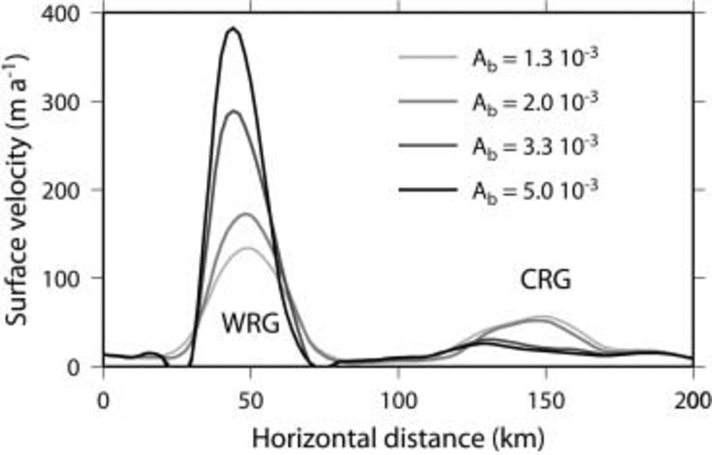
Fig. 6 Cross-section through WRG and CRG of predicted surface velocity, according to different basal sliding parameterizations.

Fig. 7. Predicted steady-state ice flux according to the basal sliding experiment with A b = 1.3 V 10-3 (a) and A b = 5.0 × 10⁻³ (b). Arrows show the direction of basal water flow.
Discussion
Reference Stokes and ClarkStokes and Clark (1999) make a distinction between pure and topographic ice streams, because an outlet glacier does not need to be associated with enhanced flow rates. Reference BentleyBentley (1987), however, claims that topographically controlled ice streams or outlet glaciers are associated with enhanced flow velocities as there is a tendency for ice flow to accelerate within topographically constrained corridors. The main reasons for occurrence of enhanced ice flow in topographic ice streams are summed up by Reference BennettBennett (2003): higher temperatures leading to enhanced ice flow are likely to occur as the ice is thicker, which allows for better isolation. Thicker ice also leads to higher driving stresses, hence higher velocities, which results in increased strain heating. Finally, most of the meltwater will be produced in these topographic lows at pressure-melting point, enhancing basal sliding. However, the whole process does not necessarily need to turn into a feedback system that leads to flow acceleration and (partial) disintegration of the ice sheet (Reference Clarke, Nitsan and PatersonClarke and others, 1977). The combined effect of basal sliding and ice softening due to thermomechanical coupling results in a relatively stable ice-sheet configuration. Even a prescribed increase in lubrication (through parameter A b) does not lead to a periodic switch between fast and slow ice flow (Reference PaynePayne, 1995; Reference PattynPattyn, 1996), nor does it lead to a switching behavior between ice streams in a time dependency, as reported by Reference PaynePayne (1998) for the Siple Coast ice streams.
Comparison of Norwegian and Belgian maps with RADARSAT imagery points to a speed-up of the ice in the western part of the Ragnhild Coast and a slow-down to the east. Although the dynamic experiments and balance-flux estimates clearly show the presence of at least two ice streams, the diagnostic experiments fail to reproduce CRG or other flow features in the east of the drainage basin. Observed inland ice velocities also show a much higher flow speed for WRG than for the adjacent CRG. Sensitivity experiments demonstrate that a speed-up of WRG causes ice piracy which eventually leads to a stoppage of CRG. In view of the above observations, such a process might already be underway.
One major distinction between an outlet glacier and the enhanced-flow zone of WRG is that the latter is not flanked by surrounding mountains. Rutford Ice Stream, for instance, is at one side flanked by mountains (and hence a real outlet glacier) but flanked by slower-moving ice at the other side (Reference BentleyBentley, 1987). WRG, by contrast, lies in a broad valley, but the fast-moving ice is flanked by surrounding slower-moving ice, and distinct shear margins can be traced all along the glacier within the ice. The fast-flow zone is not wider than 30km within a valley that is >100km wide (Fig. 8). The narrowing becomes more pronounced as basal sliding increases (Fig. 7).
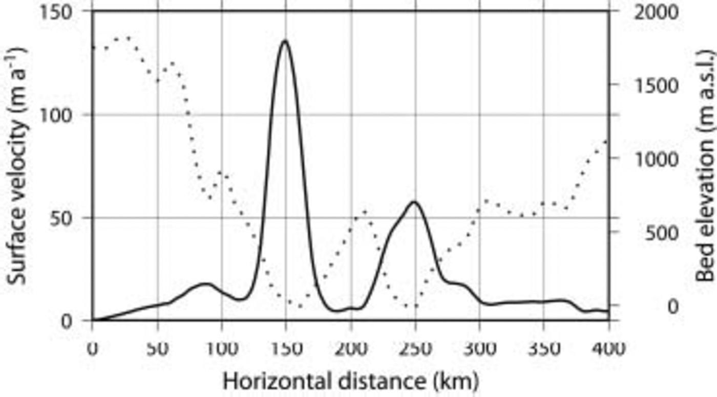
Fig. 8. Cross-section through WRG and CRG of predicted surface velocity and bed elevation.
Conclusions
Ice flow within the East Antarctic ice sheet seems rather complex, and the interior plateau is drained by large elongated features of enhanced ice flow. The Ragnhild glaciers are such features penetrating several hundred kilometers inland. Enhanced ice flow is due to thermomechanical effects and the role of basal sliding in topographic lows. Although the position of these glaciers is topographically controlled, these fast-flow zones are not flanked by rock outcrops at the surface. Hence they differ from outlet glaciers by the presence of shear margins within the ice sheet penetrating far inland. An increased lubrication of these glaciers results in ice piracy by WRG which leads to a progressive stoppage of CRG, a process that in view of observations might already be underway.
Acknowledgements
This paper forms a contribution to the Belgian Research Programme on the Antarctic (Belgian Science Policy Office), contract EV/03/08 (AMICS). S.D.B. is supported by a PhD grant of the Institute for the Promotion of Innovation by Science and Technology in Flanders (IWT). The authors are indebted to J.S. Walder and G. Flowers for their valuable help in improving the manuscript.


