

Introduction
Measurement of the seasonal cycle and interannual variations of Antarctic sea ice is important for investigations of global climate (Reference Gordon and TaylorGordon and Taylor, 1975; Reference Sturman and AndersonSturman and Anderson, 1985;Reference Allison Allison, 1989). Monitoring of sea ice is also important for ship navigation. While satellite data give a great amount of information about ice conditions (Reference Comiso and Zwally Comiso and Zwally, 1982; Reference Zwally, Comiso, Parkinson, Campell, Carsey and GloersenZwally and others, 1983; Reference Sturman and AndersonSturman and Anderson, 1985), there still remains a need for in situ validations (Reference Comiso and ZwallyComiso and others, 1984; Reference Andreas and MakshtasAndreas and Makshtas, 1985; Reference Jacka, Allison, Thwaites and WilsonJacka and others, 1987). However, visual observation of ice conditions is often difficult and is always laborious, and there is a limit to the validity of estimates of ice concentration which rely upon qualitative observation (Reference Jacka, Allison, Thwaites and WilsonJacka and others, 1987;Reference Allison Allison, 1989).
We propose a system which automatically measures the ice concentration and floe-size distribution using a computer and image digitizer. Preliminary experiments to test the system have been carried out in ice-covered water in the Southern Ocean.
System Configuration
The sea ice was photographed by a video camera mounted on board the icebreaker Shirase as shown in Figure 1. The camera was located at the upper steering house pointing at an angle of 10° downward from the horizon. The image taken by this camera is dealt with in two ways: analysis of image on line and storage of the image for analysis off line. The image is divided into 256 × 256 pixels on line or off line using an image digitizer. At each pixel location, the image brightness is quantified into 256 grey levels.
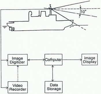
Fig. 1. System configuration for photographing sea ice. The camera was located at the upper steering house with an angle of 10° downward from the horizon.
For the on-line analysis, sea-ice images are digitized in real time. Ice concentration is calculated by summing ice pixels of each row of the digital image and ice shape can be obtained roughly by composition of the fraction of ice in each row.
For the off-line analysis, video recorded sea-ice images are processed. Both ice shape and concentration can be obtained accurately by analyzing predetermined square regions of the images.
On-Line Analysis
In order to measure the sea-ice concentration and shape in real time, one horizontal line (row) at the same position within each digital image is analyzed at predetermined time intervals as shown in Figure 2A. Since the sea-ice image is approaching the ship during navigation, orthographic projection of ice-covered water is obtained by patching the rectangular area that is composed of horizontal length of a single row and expected vertical length (Fig.2B). The vertical length is determined by the speed of the ship. The sea-ice concentration is calculated from the ratio of ice to water for each row. To reduce the processing time, images are sampled every second, thus each floe is composed of rough rectangular arrays of pixels.
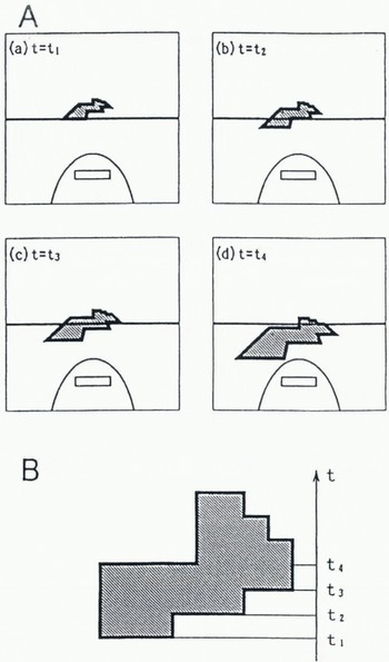
Fig. 2. Schema of composition of sea ice. The floe representation, B, is composed of the fraction of ice on each row in A. Since images are sampled at fixed finite intervals, they are composed of roughly rectangular arrays of pixels.
If the speed or course of the ship is changed, the shape of the floe is distorted. Although some limitations exist, ice concentration and rough floe size can be obtained in real time by this analysis.
Off-Line Analysis
Figure 3A shows the spatial relation between the sea surface and its projection in the image plane. Using known lengths and angles such as camera height, distance from camera to bow and angle of depression of the camera, a geometric transformation is performed. By this transformation, a square region of sea with a side of 180 m is analyzed, and each image of sea ice (Fig.3b) is transformed to an orthographic projection (Fig.3c). In the geometric operation, the output pixels are mapped into the input image to establish their grey level. If an output pixel falls between four input pixels, interpolation is necessary to determine the grey level of the output pixel (Reference CastlemanCastleman, 1979). In this process, as the distance from the ship increases, the area of a pixel increases, and the accuracy of the area of remote pixels lessens.
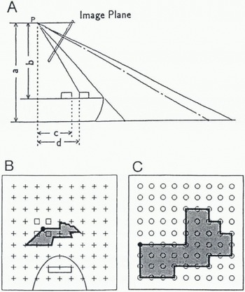
Fig. 3. Schema of geometric transformation. A, spatial relation between the sea water and its projection in the image plane. Using known lengths (a-d) and angles, geometric transformation is performed. B, oblique projection. C, orthographic projection transformed from trapezoid region shown in B on oblique projection. The grey levels of input image B are transferred to the output image C pixel by pixel. If an output pixel (•) maps to a position between four input pixels (□), then its grey level is divided among the four input pixels according to the interpolation rule.
Transformations
The spatial transformation
The general definition for a geometric operation is
, where f(u, υ) is the input image and g(u′, υ′) is the output image as shown in Figure 4. The functions a(u, υ) and b(u, υ) uniquely specify the spatial transformation. In the input image f(u, υ) the grey-level values are defined only at integral values of u and υ. However, this equation will in general dictate that the grey level value for g(u′, υ′) be taken from f(u, υ) at non-integral coordinates. As mentioned previously, the output pixels map to fractal position in the input image, generally falling in the space between four input pixels. Interpolation is necessary to determine the grey level of the output pixel.
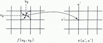
Fig. 4. The spatial relationship between points in the input image and points in the output image. The output pixels are mapped into the input image. If an output pixel maps to a position between four input pixels, then interpolation is necessary to determine the grey level of the output pixel.
Nearest-Neighbor Transformation
The simplest interpolation scheme is the so-called zero-order or nearest-neighbor interpolation. In this case, the grey level of the output pixel is taken to be that of the input pixel nearest to the position to which it maps as shown in Figure 5A. This is computationally simple and produces acceptable results in many cases. However, nearest-neighbor interpolation can introduce artifacts in images containing fine structure whose grey level changes significantly over one unit of pixel spacing.
Bilinear Transformation
First-order interpolation produces more desirable results with a slight increase in programing complexity and execution time. In Figure 5B, let f(u 0, υ 0) be a function of two variables that is known at (u′, υ′), (u′, + 1 υ′), (u′, υ′ + 1) and (u′ + 1, υ′ + 1), which are the vertices of the unit square. Suppose we desire to establish the value of f(u 0, υ 0) at an arbitrary point inside the square by interpolation through the four known values. We shall do so by fitting a hyperbolic paraboloid, defined by the bilinear equation
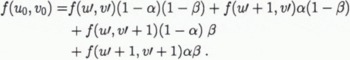
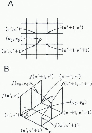
Fig. 5. Grey-level interpolation. A, nearest-neighbor interpolation. In this case, the grey level of the output pixel is taken to be that of the input pixel nearest to the position to which it maps. B, bilinear interpolation. In this case, the grey level of the output pixel is determined by the bilinear equation using the known values at four corners.
An Example of Sea-ice Images with Transformations
Figure 6 compares bilinear with nearest-neighbor transformation. In these photographs, white areas indicate ice and black areas indicate water. The trapezoid region of ice-covered water in Figure 6A, transformed to an orthographic projection by nearest-neighbor and bilinear interpolation procedures, is shown in Figure 6B and D. To separate ice from sea water, the transformed images are converted to a binary image by a suitable grey-level threshold, as shown in Figure 6C and E. The threshold level was determined using a grey-level histogram of the image at the beginning of the analysis, and this level was fixed. Although we examined some points for the effect of threshold level, almost all separated satisfactorily except the case of back lighting from the sun. In Figure 6C a sawtooth effect appears at some of the edges. In Figure 6E desirable result is obtained. The ice concentration is calculated by summing ice pixels over the 180 m × 180 m area to get a regional measure. Floe size could be determined only for floes completely contained within an image. Though bilinear transformation requires much calculation, this method is useful for detailed analysis of regional ice properties.
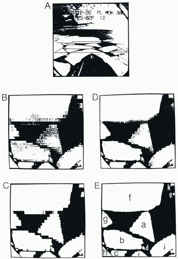
Fig. 6. Comparison of nearest-neighbor and bilinear interpolation. A, an original image. The trapezoid region on ice-covered water was transformed to orthographic projection by nearest-neighbor (B) and bilinear (D) interpolation. C,E, binary image of B and D, respectively.
Results
The sea-ice image was recorded between Fremantle, Australia, and Syowa Station in 1988 by T. Endoh, a member of the 30th Japanese Antarctic Research Expedition (JARE-30). The cruise track of the icebreaker Shirase from Breid Bay to Syowa Station is shown in Figure 7.
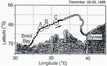
Fig. 7. Cruise track of the icebreaker Shirase every hour (solid and open square) from 26–29 December 1988.
On-line analysis was performed at predetermined time intervals using the images photographed during navigation. The ice concentration and shape were analyzed every second as shown in the example at Figure 8, and the data were stored. Figure 9A shows changes of ice concentration estimated every 5 s during the first 24 h from Breid Bay to Syowa Station. Figure 9B depicts 10 min running means of the ice concentration. These graphical records are useful to examine the general tendency of ice concentration during the observation. Because the vessel navigates to find the easiest passage, the ice concentration may be biased towards a lower limit. The differences between ice concentrations along the route and in neighboring regions must be identified by alternative methods, such as by observation from helicopter or by remote sensing.
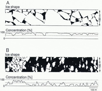
Fig. 8. Examples of ice concentration and shape resulting from analysis every second. Mean ice concentrations during 5min intervals shown were 81.6 % in A and 29.0 % in B.
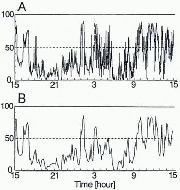
Fig. 9. Changes of ice concentration during the first 24 h from Breid Bay to Syowa Station (solid squares shown in Fig. 7). A, estimated every 5s; B, 10min running mean.
Table 1 shows the 11 floe sizes of Figure 6E. While floes a-e were surrounded by water on the image display, allowing calculation of floe area, floes f-k were not. Figure 10 shows the floe-size distributions calculated for the areas A, B and C of Figure 7. In some cases, the ice concentrations had almost the same value but the distributions of floe size were different. Figure 10A and C shows an example of such a case: a large area of ice but a small number of floes in Figure 10A and vice versa in Figure 10C.
Table 1 Floe size of Figure 6E
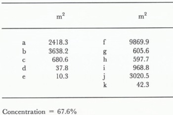
Concentration = 67.6%
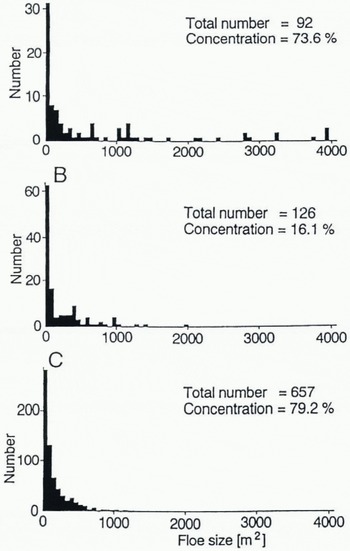
Fig. 10. Floe-size distribution for the three areas A, B and C of Figure 7. Although the ice concentrations had almost the same value in A and C, distributions of floe nze were different.
During on-line analysis, the data from time series analysis of the ice concentration will be useful for investigation of long-term variations (Fig. 9). In this analysis, however, the ice shape cannot be obtained with accuracy. In the off-line analysis, both ice shape and ice concentration can be accurately obtained by analyzing predetermined square regions of an image (Fig.6 and Fig.10). Although the off-line method requires more time to calculate, it is useful for detailed analysis of regional ice properties. It follows from these results that choice of analysis depends on purpose.
Conclusion
The system for analyzing sea-ice concentration and floe-size distribution offers several practical advantages. Chief among these are: (1) All the hardware components are commercially available. (2) The system is easy to use. (3) The software can easily be adapted to an image photographed from another camera position. (4) On-line or off-line analysis can be utilized depending on the purpose. (5) Furthermore, this technology will be easily applied to images obtained in other ways such as from helicopters or aircraft.
Acknowledgements
The authors thank M. Kosugi for development of software.


