List of Symbols

a Arrhenius constant (Pa⁻ⁿ a⁻¹)

A Ice flow-law parameter (Pa⁻ⁿ m⁻ⁿ a⁻¹)

A _s Sliding-law parameter

b Flow-band width (m)

c _p Specific heat capacity (J kg⁻¹ K⁻¹)

D Diffusion coefficient (m² a⁻¹)

g Gravitation constant (9.81 ms⁻²)

G Geothermal heat flux (−54.6 m W⁻²)

h Bedrock elevation above present sea level (m)

H Ice thickness (m)

k _i Thermal conductivity of ice (J m⁻¹ K⁻¹ a⁻¹)

L Specific latent heat of fusion (3.35 × 10⁵ J m⁻¹ K⁻¹ a⁻¹)

m Flow-enhancement factor

M Surface mass balance (ma⁻¹ ice equivalent)

N Effective normal pressure (Pa)

n Glen flow-law exponent (3)

p Sliding-law coefficient (0–3)

P _g Pressure gradient (Pa m⁻¹)

q Sliding-law coefficient (0–2)

Q Activation energy for creep (J mol⁻¹)

Q _w Water flux (m³ s⁻¹)

R Universal gas constant (8.314 J mol⁻¹ K^–1)

R _ij Resistive stress (Pa)

S Basal-melting rate (m a⁻¹ ice equivalent)

t Time (a [year])

T Ice temperature (K)

T ₀ Absolute temperature (2730.15 K)

T^* T relative to pressure melting (K)

u Horizontal velocity (m a⁻¹)

u _s Basal-sliding velocity (m a⁻¹)

U Vertical mean velocity (m a⁻¹)

w Vertical velocity (m a⁻¹)

x Horizontal coordinate (m)

z Vertical coordinate (m)

β Geometric constant (≈2.0)

δ Water-film depth (m)

δ _e Critical particle size (m)

δ _ij Kronecker delta

Δ _ζ Horizontal gradient at depth ζ

ϵ Effective shear-strain rate (a⁻¹)

ϵ Shear-strain rate (a⁻¹)

γ _g G/k _i (geothermal heat) (K m⁻¹)

κ Boundary value (0 (surface) or 1 (bottom))

Λ Lithostatic stress component (Pa)

μ Viscosity of water (1.8 × 10⁻³ Pa s)

ρ Ice density (910 kg m⁻³)

ρ _s Sea-water density (1028 kg m⁻³)

σ _n Normal stress at the base (Pa)

σ _b Ice-shelf back-pressure (Pa)

υ Temperature-correction factor (0.0–0.1 ° C⁻)

τ _b Basal shear stress (Pa)

τ _e Effective stress (Pa)

τ _d Driving stress (Pa)

τ _ij Stress (Pa)

τʹ_ij Stress deviator (Pa)

ζ Vertical dimensionless coordinate

Introduction

The dynamic behaviour of a large polar ice sheet is well understood; grounded ice flow is basically governed by shearing close to the bed. In its most simplistic form, the basal shear stress equals ice density times gravity times overburden depth times surface slope, which Hutter (1993) defined as the glaciologist’s first commandment. However, like any physical system, an ice sheet is not only controlled by its internal dynamics but also by its boundary conditions, which are less well understood. The environmental processes such as surface temperature and mass balance act as the upper boundary and are in many ice-sheet models regarded as the external system forcing. The present environmental conditions thereby serve as a reference. The two remaining boundaries, on which we will further concentrate in this paper, are the basal motion as a lower and the margin dynamics as the outer boundary condition. The basal velocity depends on the internal ice dynamics, the bedrock conditions and the presence of water at the ice-sheet base. Basal velocity will thus play a role when the temperature of the basal ice is at the melting point and will gain more importance close to the margin where it interacts with the margin ice dynamics.

When the ice-sheet margin terminates at the sea in the form of a floating ice shelf, a transition zone can be defined where the ice-sheet dynamics gradually evolve towards ice-shelf dynamics. Elaborate studies on this grounding zone have revealed that for small basal motion the width of the transition zone is of the same order of magnitude as the ice thickness, so that the grounding zone is reduced to a grounding line and the shallow-ice approximation still holds, provided that there is no passive grounding of the ice shelf. A full derivation of the Stokes balance equations is not necessary; it suffices to calculate the longitudinal stress deviator along the grounding line and prescribe a longitudinal stress gradient (Van der Veen, 1987). Grounding-line movement is thus only governed by ice-sheet mechanics (Hindmarsh, 1993). This situation is the commonest outer boundary at the edge of the East Antarctic ice sheet where a steep surface slope, characterizing grounded ice, abruptly changes to a small surface gradient where the ice begins floating.

However, large amounts of Antarctic ice arc not drained along these margins but through fast outlet glaciers or ice streams, which are believed to be more sensitive to environmental changes. These ice streams are characterized by large basal velocities, relatively small surface gradients and a low basal traction. The internal ice dynamics involve not only shearing but also long-itudinal stretching, thus violating the first commandment. In West Antarctica, where ice streams are a common drainage feature, they are able to destabilize the ice sheet.

The East Antarctic ice sheet is also in some places drained by large ice streams, such as Lambert Glacier, Jutulstraumen, Shirase Glacier or Slessor Glacier. In this paper we will focus on Shirase Glacier (70° S, 39° E) in Enderbv Land (Fig. 1). This important continental ice stream drains about 90% of the total ice discharge of the Shirase Drainage Basin covering approximately 200 000 km². This S-shaped basin extends from the polar plateau near Dome F (77°22′S, 39°37′E) to Lützow-Holmbukta. Shirase Glacier is one of the fastest-flowing Antarctic glaciers, with velocities up to 2700 m a⁻¹ in the ice-stream region (Fujii, 1981). The ice flow in the central drainage basin is furthermore characterized by large submergence velocities (Naruse, 1979}. Consecutive measurements in this area (Naruse, 1979; Nishio and others, 1989; Toh and Shibuya, 1992) have pointed to a large thinning rate ranging from 0.5 to 2.0 m a⁻¹ in the region where the surface elevation is lower than 2800 m. Kameda and others (1990) concluded from a study of the total gas contents of ice cores in this area that the thinning is a rather recent phenomenon and that the ice-sheet surface decreased by about 350 m during the last 2000 years.

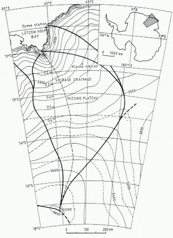
Fig. 1. Location map of Shirase Drainage Basin. The dashed line represents the central flowline, as primary input for the modelling experiments. The flowline starts tit Dome F, follows more or less the 40° E meridian towards Lützow-Holmbukta, and ends at Shirase Glacier in a floating ice tongue.

In a previous paper, Pattyn and Decleir (1995) simulated the dynamical behaviour of the Shirase Drainage Basin during the course of the last glacial-interglacial cycle. Except for the ice-stream area, the model was able to describe the main features of the drainage basin. The present paper focuses on the processes in the ice-stream area and near the basal boundary, which we think are important in controlling the enhanced thinning of the ice sheet. First, the present force balance of the ice-stream area is calculated progressively from the surface of the present ice sheet (as displayed in figure 2a; using the observed surface velocity as an upper boundary) to the bottom, according to the method proposed by Van der Veen and Whillans (1989). This experiment is described in the section “Diagnostic model run”. Secondly, by inverting this method, the total stress-field derivation is incorporated in an ice-sheet system model, where the calculations start at the bottom (basal velocity) and progress towards the ice-sheet surface, as explained by Van der Veen (1989). In the latter case, sensitivity experiments are carried out with different descriptions of the basal motion in order to understand the ice-sheet response with time. Therefore, we took a simple ice-sheet configuration as given in Fig. 2b, in order to reduce local effects imposed by the Shirase Glacier bedrock topography. An S-shaped basin form was kept to take into account the large convergence in the ice-stream area.

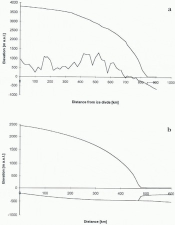
Fig. 2. Geometric characteristics of the Shirase Glacier flowline (a) and the steady-state reference ice sheet for the modelling experiments (b).

Velocity and Stress-Field Calculation

The numerical ice-sheet system model used in this study is a dynamic flowline model that predicts the ice-thickness distribution along a flowline in space and time as well as the two-dimensional flow regime (velocity, strain rate and stress fields) and temperature distribution in response to environmental conditions.

A Cartesian coordinate system (x, z) with the x axis parallel to the geoid and the z axis pointing vertically upwards (z = 0 at sea level) is defined. Starting from the known bedrock topography and surface mass-balance distribution, and assuming a constant ice density, the continuity equation is used to form an evolution equation for the ice thickness H where

(1)

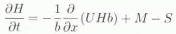
with U the depth-averaged horizontal velocity, H the ice thickness, M the surface mass balance and S the melting rate at the base of the ice sheet. Divergence and convergence of the ice flow are taken into account in the calculation of the variation of the ice flux along the flowline through the parameter b, indicating the width of the flow band and taken perpendicular to the flowline. Boundary conditions to the ice-sheet system are zero surface gradients at the ice divide and a floating ice shelf at the seaward margin.

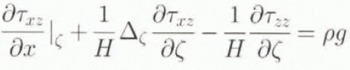
For the derivation of the two-dimensional stress field in the ice-sheet system, the method described by Van der Veen and Whillans (1989) and Van der Veen (1989) was followed as the main reasoning. For numerical convenience, a dimensionless vertical coordinate is introduced to account for ice-thickness variations along the flowline, which is defined as ζ = (H + h − z)/H, so that ζ = 0 at the upper surface and ζ = 1 at the base of the ice sheet. The major assumption made in the model formulation is to consider plane strain, so that all stress components involving y are neglected. In this way, the Euller continuum in two dimensions is written as

(2a)

(2b)

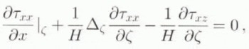
where

(3)

Following Whillans (1987) and Van der Veen and Whillans (1989), the full stress components from Equation (2) are partitioned into a resistive (R_ij ) and and a lithostatic (Λ) component, so that

(4)

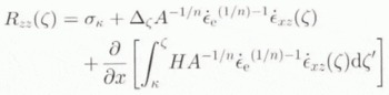
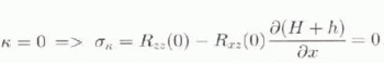
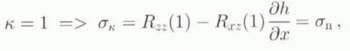
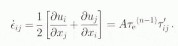
with δ_ij the Kronecker delta, equalling 1 when i = j and 0 otherwise. Introducing the resistive-stress component into Equation (2b) and integrating from the boundary κ to a general depth ζ in the ice sheet results in an expression for the resistive-shear stress. The boundary value κ is introduced so that calculations can start from the surface (κ = 0) as well as from the bottom (κ = 1) of the ice sheet. The starting condition κ = 0 is applied in the diagnostic run. (see later) while the starting condition κ = 1 is used in the modelling experiments. Resistive Stresses can then be replaced by shear-strain rates through the constitutive relation and the relation between the full stress tensor and the deviatoric stress. Glen’s flow law is used as a constitutive relation (Paterson, 1994). The resulting equation then becomes (Van der Veen and Whillans, 1989; Van der Veen, 1989)

(5a)

(5b)

(5c)

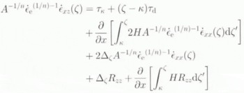
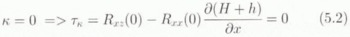
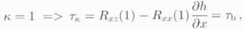
where τ_d is the driving stress (τ_d = − ̜gH ߜ (H + h)). Equation (5a) can be integrated numerically from the surface (κ = 0) or from the bottom (κ = 1) of the ice sheet with boundary conditions (5.2) and (5.3), respectively. The flow-law parameter A is a function of temperature T* (corrected for the dependence of the melting point on pressure (T* = T ₀ − (8.7 × 10⁻⁴)H}) and obeys an Arrhenius relationship (Paterson, 1994):

(6)

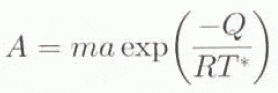
where a = 1.14 × 10⁻⁵ Pa⁻ⁿ a⁻¹ and Q = 60 kJ mol⁻¹ for T* < 263.15 K, a= 5.74 × 10¹⁰ Pa⁻ⁿ a⁻ and Q = 139 kJ mol⁻¹ for T* ≥ 263.15 K.

An expression for the vertical resistive stress is obtained by vertically integrating Equation (2b) from the surface to a depth in the ice sheet ζ. After algebraic manipulation similar to the derivation of Equation (5), the vertical resistive stress can be written as:

(7a)

(7b)

(7c)

where Equations (7.2) and (7c) apply to the boundary conditions at the surface or at the bottom, respectively. Strain rates are by definition related to velocity gradients, such that

(8)

Introducing the scaled vertical coordinate system and applying the incompressibility condition (∂u/∂x + ∂w/∂z = 0), an expression can be found for the normal strain rate in the horizontal direction. Boundary conditions to this system of equations are a stress-free surface and known horizontal and vertical ice velocities at the surface or at the basal layer. The whole velocity field can be calculated from the ice-sheet geometry, taking into account the proper boundary conditions. The numerical solution to the above-described equations has been explained in Van der Veen (1989) and briefly hereafter. Once the two-dimensional velocity held is calculated, horizontal ice fluxes, which are related to the rate of ice-thickness change through Equation (1) are found by integrating the horizontal velocity from the bottom of the ice sheet to the surface, hence

(9)

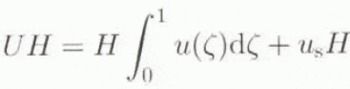
where u _s is the basal-sliding velocity, which will be defined later.

ICE Temperature and Isostatic Bedrock Adjustment

The temperature distribution in an ice sheet is governed both by diffusion and advection, and is therefore dependent not only on boundary conditions such as surface temperature and geothermal heat flux but also on ice velocity. The thermodynamic equation can thus be written as (Huybrechts and Oerlemans, 1988; Ritz, 1989)

(10)

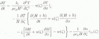
with T temperature and k _i and c _p the thermal conductivity and the specific heat capacity, respectively. The heat transfer is thus a result of vertical diffusion, horizontal and vertical advection and internal deformation caused by horizontal shear-strain rates. Boundary conditions follow from the annual mean air temperature at the surface and the geothermal heat flux (enhanced with heat from sliding) at the base (Ritz, 1987) so that

(11)

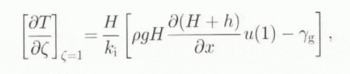
where γ_g is the geothermal heat entering the ice at the base and taken as a constant for the line of experiments discussed here. The basal temperature in the ice sheet is kept at pressure-melting point whenever it is reached and the surplus energy is used for melting. This may, in some cases, lead to the formation of a temperate ice layer between Ϛ = 1 and Ϛ = Ϛ_melt, so that the basal-melt rate S is defined as

(12)

where index b denotes the basal temperature gradient as given in Equation (11) and index c denotes the basal temperature gradient after correction for pressure melting. In the ice shelf, the vertical temperature profile is taken linearly with the surface temperature as the upper boundary condition and a constant temperature of −2°C at the bottom of the ice shelf. Melting or refreezing processes at the ice-sea-water contact are not taken into account.

Bedrock adjustment to the ice load is calculated as described by Oerlemans and Van der Veen (1984, chapter 7). The elastic properties of the lithosphere determine the ultimate bedrock depression, while the viscosity of the underlying astenosphere determines the relaxation time. The time-dependent response is modelled by a diffusion equation for bedrock elevation.

Numerical Solution

The main part of the numerical scheme consists of solving the balance Equation (5) for the shear-strain rate at general depth ζ. Therefore, velocities at that depth layer and the velocities of the layer underneath or above need to be known. For modelling purposes, integration starts at the bedrock (κ = 1), conditioned by a basal velocity and which is governed by both basal sliding mechanisms, ice-stream and ice-shelf flow. Furthermore, the basal velocity is influenced by the two-dimensional stress field and vice versa, so that linking of the two mechanisms should be performed dynamically. Van der Veen (1989) offered a solution for the integration of the flow field starting from the bed. The numerical computation is, however, rather time-consuming and increases when eventually a basal boundary condition is linked to the flow field. However, by choosing good initial estimates to the basal drag and normal stress, convergence can be attained rather rapidly, even when basal velocity is influenced by the basal drag. The final flow-field determination is stopped when the stress-free surface condition is fulfilled, i.e. Equations (5c) and (7c).

The two-dimensional ice-sheet system model is implemented on a flowline which extends from the ice divide to the edge of the continental ice shelf. Because of the non-linear nature of the velocity in the ice sheet, the continuity Equation (1) is reformulated as a non-linear partial differential equation and written as

(13)

with D(x) a diffusion coefficient which, in the grounded ice sheet, equals the mass flux (UH) divided by the surface gradient. A solution to this equation can be obtained by writing Equation (13) in the conservation form (Mitchell and Griffiths, 1980). For the numerical computation, a semi-implicit scheme was applied and new ice thicknesses on the next time step are found by the solution of a tri-diagonal system of equations. An implicit numerical scheme was adopted for the ice-temperature field, resulting in a similar set of tri-diagonal equations.

Diagnostic Model Run

The ice-sheet geometry of Shirase Drainage Basin (surface and bedrock elevation) was compiled from Japanese topographic maps of the region. Surface velocities are known at several sites on Mizuho Plateau and at the glacier margin. More detailed reference to the compilation of the flowline data, present mass-balance and surface-temperature distribution can be found in Pattyn and Decleir (1995). Temperature in the ice sheet was calculated on the basis of a steady-state temperature distribution and coupled to the velocity field by means of the Arrhenius relationship.

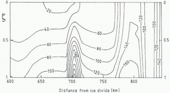
Fig. 3. Two-dimensional map of the effective stress field in the downstream area of Shirase Glacier.

Adopting this ice-sheet configuration, it was possible to obtain the two-dimensional stress and strain field in the ice sheet, from the ice divide to the edge of the floating ice shelf, simply starting from the present horizontal and vertical surface velocities, The present surface mass balance was used as the upper boundary to the vertical velocity. The resulting effective stress distribution (incorporating both shearing and stretching) in the glacier area (from a distance of 600 km from the ice divide down io the grounding line) is displayed in Figure 3. In the upstream area, the ice flow is primarily governed by shear stresses (down to 710 km from the divide), because of the relatively high surface slopes imposing a large driving stress. The ice-stream area itself (from 800 km further downstream) is almost solely driven by longitudinal stretching and shear stresses are almost negligible. Between these two areas both shear stress and longitudinal stress are of the same order of magnitude and form some kind of transition zone. Despite the poor knowledge of the detailed surface and bedrock topography and surface velocities in the ice-stream area (700–850 km from the divide), Figure 3 depicts the overall characteristics of an ice stream, i.e. a large horizontal velocity gradient and a very small vertical gradient of the horizontal velocity (∂u/∂z ≈ 0). These features more resemble ice-shelf behaviour than grounded ice-sheet dynamics.

Vertical resistive stresses play a role in those areas where the flow regime changes, i.e. from shearing to stretching and vice versa. They are of the order of 1–5 k Pa, almost two orders of magnitude smaller than the effective stress.

Basal Velocity

For modelling purposes, the full stress field in an ice-sheet system, which consists of a grounded ice sheet, its grounding zone or ice-stream area and a coupled ice shelf, is derived starting from a basal boundary condition. The calculation of the two-dimensional ice-velocity field is thus reduced to a one-dimensional problem, in which the basal-sliding mechanism in the ice sheet, the ice-stream flow mechanism and the ice-shelf flow needs to be determined. Since the basal boundary condition is iteratively updated with the derivation of the two-dimensional flow field, the final solution is a two-dimensional one.

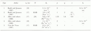
Table 1.1 Constants and parameters for the different basal velocity laws. HAB = effective normal pressure calculated from the height above buoyancy (see text). The numbers between brackets refer to the equation in the text

The ice shelf is simply taken as a freely floating ice shelf bounded in a parallel-sided bay, so that all stresses in the y direction can be set to zero. Vertical shearing is omitted, so that the force balance equation reduces to

(14)

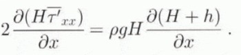
In order to calculate the longitudinal deviatoric stress from this equilibrium, its value at the seaward edge of the ice-shelf must be known. Here, the total force of the ice must be balanced by the sea-water pressure (Thomas, 1973), so that

(15)

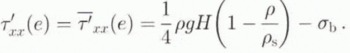
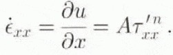
Using this expression to calculate the longitudinal stress deviator at the edge of the ice shelf, Equation (15) is then integrated upstream to yield the longitudinal deviatoric stress in the whole ice shelf. Once the vertical mean horizontal velocity at the grounding line is known, the vertical mean horizontal ice-shelf velocity (which equals the basal velocity) is calculated from the definition of the normal strain rates and the constitutive relation:

(16)

The temperature-dependent flow-law parameter A is taken as a constant in the whole ice shelf, based on the mean ice-shelf temperature.

Basal sliding of the grounded ice sheet can originate from sliding of the ice over its bed and deformation of the bed itself, the latter if the bed consists of sediments saturated with water at a pressure that closely matches the ice-overburden pressure. Sliding is thus only expected where the basal ice is at the melting point (Paterson, 1994). In polar ice streams, the origin of the basal water is most likely due to basal melting primarily caused by strain heating. Percolation of surface meltwater and the formation of intraglacial channels and moulins might thus be neglected. In most sliding laws, derived from laboratory experiments and data fitting from observed values, basal sliding is a function of the shear stress at the base, bed roughness and the effective normal pressure at the base, the latter equalling the ice-overburden pressure minus the water pressure at the base of the ice sheet. A general sliding law has the form of (Bindschadler, 1983; Budd and others, 1984; Budd and Jenssen, 1987; Van der Veen. 1987)

(17)

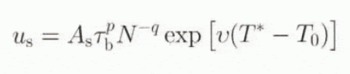
where p and q are positive numbers ranging between 0 and 3 and the exponential term a correction for the basal temperature, introduced by Budd and Jenssen (1987). For glaciers that terminate in the sea, subglacial water pressure at the grounding line may be calculated from the flotation criterion, so that the effective normal pressure N is proportional to the height of the glacier surface above buoyancy. In some flow models of the Antarctic ice sheet (Budd and others, 1984; Huybrechts, 1990), the effective pressure is calculated in the same fashion over the whole model domain and not only at the grounding line. However, the physical restriction is that the bedrock should lie below sea level and that the water pressure originates from sea water infiltrating at the grounding line and moving in the upstream direction. Since this type of parameterization is widely used in ice-sheet models, it is adopted for the calculation of sliding type 2 and 5 in Table 1 (denoted by HAB).

Subglacial water pressure or the pressure gradient underneath the ice sheet can be derived from the existence of subglacial channels and/or cavities. Bindschadler (1983) applied the so-called Röthlisberger-channels (Röthlisberger, 1972) for the derivation of effective normal pressure in Antarctic ice streams. The theory and physical background of the formation of channels and cavities is very complicated and is highly dependent on the detailed bedrock topography (bumps). Since basal condition at Shirase Glacier are hardly known, the use of such physical principles remains highly speculative.

A more straightforward treatment of the basal water flow is to consider a water film underneath the ice sheet. According to Weertman and Birchfield (1982), the sliding velocity is dependent on the depth of the water layer δ and the critical particle size δ_c so that

(18)

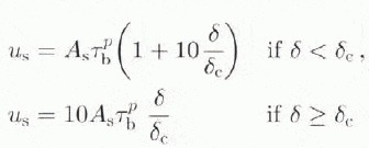
and

(19)

where Q _w is the water flux per unit width, calculated through downstream integration of the basal melting rate and P _g the pressure gradient (Alley, 1989).

In the analysis above, the glacier moves over an undeformable bed, and the water acts as a lubrication layer between the bedrock and the ice. However, in the presence of subglacial till, it is very likely that, whenever this till layer becomes saturated, the drainage is along the till and/or bed (Walder and Fowler, 1994). When the till layer is sufficiently thick, deformation of the till layer (bed deformation) can occur (Alley, 1989). Combination of all these processes (cavities in ice and till, subglacial aquifers) obviously makes the basal sliding mechanism very complicated. Nevertheless, Alley and others (1989) incorporated in a simplified way the bed deformation. Neglecting the shear strength of the till and setting the effective pressure (N) independent of depth, the bed-deformation velocity then takes the form of the sliding velocity Equation (17) without the exponential term. The effective pressure (N) is calculated as (Alley and others, 1989)

(20)

where the denominator represents the fraction of the bed occupied by the water film with depth δ, and β a geometric constant related to the bed roughness (β ≈ 2.0 in the analysis of Alley and others (1989)).

In total, we considered live different basal velocity laws, based on three different basal movement concepts: (i) basal sliding related to basal shear stress and effective normal pressure at the bed, (ii) sliding due to the presence of a water him and (iii) till deformation at the ice bed interface. The coefficients for the different basal-motion laws are given in Table 1.

Sensitivity Experiments

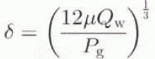
For the standard model run, no considered a linear sloping bedrock, with an elevation of 500 m a.s.l. at the divide, away from it gradually lowering by 150 m per 100 km, and a horizontal grid size spacing of 10 km. In the vertical domain, 20 layers were defined with the lower layer spacing of Δζ = 0.015, gradually increasing towards the top. Starting from the initial bedrock condition, we developed an ice sheet bounded by the surface mass balance and temperature configuration as obtained from data of Shirase Drainage Basin (Pattyn and Decleir, 1995). Taking this simple bedrock topography, local extraneous effects interacting with the basal motion laws are excluded. Only an S-shaped basin form and the upper boundary (surface mass balance and temperature) are in accord with the present observations. After 40 000 years of calculation a full-grown steady-state ice sheet was obtained with a bedrock lying approximately 400 m below sea level (due to bedrock adjustment) and a temperature field coupled to the velocity field. Basal velocity was excluded from this standard run. The grounding line was situated at a distance of 470 km from the ice divide and determined by the flotation condition (Fig. 2a). Using this steady-state situation as a reference, the model ran forward again 20 000 years constrained by one of the five selected basal motion laws, According to Figure 4, the proportion of basal movement in the total balance velocity is highly dependent on the basal motion type. Basal-sliding types 2, 4 and 5 show a gradual increase in the proportion of basal motion in the total velocity towards the grounding line. These are the Budd and Van der Veen type based on Equation (17), with the effective pressure independent from the water production at the ice-sheet base, and the Alley type for a water film (Equation (18)). These three types are a function of the basal shear stress, which increases towards the grounding line. However, the till-deformation law (type 3) also depends on the basal shear stress, as can be seen in Table 1 but, looking closely at the governing equations for this type, one notices that the basal shear stress also enters the effective pressure (N) through Equation (20), so that the basal motion in fact becomes inversely proportional to the basal-shear stress due to the power constants p and q (1.33 and 1.8, respectively). The remaining types 1 and 3 (sliding over a water film and till deformation) are characterized by a sudden increase in basal velocity where the basal-ice temperature reaches the pressure-melting point, and the proportion of the basal motion in the total velocity decreases in the downstream direction. Both experiments create an ice sheet with a disturbance in the surface-topography profile at the place where the basal-ice temperature reaches the pressure-melting point, thus creating a kind of enhanced “block-flow” movement of the downstream part of the ice sheet. Al the cold/temperate interface, the ice is “sucked” out of the upstream ice sheet, resulting in a smaller surface gradient and a non-neglectable importance of the longitudinal stress.

A question that arises when the ice sheet is subjected to a change in basal boundary conditions is whether or not the ice mass will retrieve a new steady state. The answer is given by Figure 5, displaying the mean grounded-ice thickness during the course of 20 000 years of integration for the five basal motion experiments. Whenever the basal movement cannot be balanced by the ice input upstream (and surface mass balance), the ice sheet will continuously shrink, given that the environmental condition remains the same or favours the enhanced basal movement (such as a warmer climate). However, the ice-sheet temperature plays an important role in controlling the basal ice-sheet dynamics. Introducing basal movement causes the ice sheet to move more rapidly, hence increasing horizontal and vertical advection rates. Colder temperatures reach the base of the ice sheet, thus decreasing the total surface subjected to melting. Basal velocities decrease, stabilizing the ice-sheet motion. The whole process gives rise to a cyclic behaviour; the slower ice sheet will tend to grow, advection rates decrease, bottom melting increases, hence resulting in larger basal velocities. This can be seen in Figure 6, where both mean ice thickness and temperature change during the course of 20 000 years are displayed, according to the basal-sliding type 1. In particular, the sliding laws which are directly dependent on the changing basal characteristics such as the basal-melting rate will show this apparent behaviour. Furthermore, when basal-velocity gradients increase, stretching becomes the dominant process, so that shearing in the basal layers becomes less effective (∂_u/∂_z ≈ 0), thus reducing the production of basal meltwater caused by strain heating. The amount of basal meltwater influences directly the basal-water flux and the sliding velocity.

Fig. 4. Ratio of the basal velocity to the total balance velocity in the ice sheet according to the five types of basal velocity laws after 20 000 years of integration (see text for explanation).

Discussion

Payne (1995) showed the existence of cyclic behaviour in ice sheets with a thermomechanical ice-sheet model using a basal sliding mechanism similar to the Budd sliding type 2 in this paper. He found that the coupling of the ice-flow field and the temperature evolution gives rise to limit cycles in the basal thermal regime of the ice sheet. These cycles are caused by the switching on and off of sliding as basal ice reaches the pressure-melting point. Results of our work do not show this cyclic behaviour for a sliding law in which the effect of basal water is not explicitly included. This is probably due to a lower tuning value in our experiments compared to the sliding law of Payne (1995). By comparing different basal-motion laws, it seems that those which depend on basal water are much more sensitive to this cyclic response, because they not only invoke an on-and-off switching when basal ice reaches the pressure-melting point but the basal-motion magnitude is also directly influenced by the amount of meltwater produced at the base. Basal meltwater depends both on the basal temperature and velocity gradients, which enhances the complexity of the interaction process.

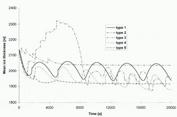
Fig. 5. Evolution of the mean grounded ice thickness when applying the five different basal velocity laws.

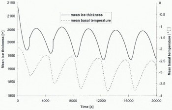
Fig. 6. Evolution of the mean grounded ice thickness and mean basal temperature when applying basal sliding type 1.

These simple comparison experiments showed that regardless of climatic variability, an internal oscillation mechanism is generated due to the interaction between the ice-sheet thermomechanics and the basal processes and that basal processes such as sliding over a water film, buoyancy at the grounding area and till deformation cause a different response in ice-sheet behaviour. In the future, we will therefore carry out elaborate sensitivity experiments in order to explain the amplitude and periodicity of these cyclic events in view of the basal mechanisms and external forcing such as mass balance and surface temperature.

Conclusions

Based on the present ice-sheet configuration, mass balance and surface temperature, the internal stress distribution of Shirase Glacier was analysed by the method proposed by Van der Veen and Whillans (1989). Despite the lack of detailed measurements in the ice-stream area, the main properties of the stress field could be revealed. For a distance down to 700 km from the ice divide, the ice-sheet mechanics are solely driven by shearing in the lower layers. Further downstream continues a transition zone where both shearing and stretching play an equal role, about 200 km in length, which is followed by an ice-stream zone 50 km in length where gradually the basal-shear stress lowers to become zero in the ice shelf.

The numerical analysis showed that the interaction between basal velocity and ice dynamics in fast-flowing ice sheets is very complicated and its effect can only be understood with time-dependency. In the applied numerical model, the full Stokes equations were taken into account and the velocity field coupled to the ice-temperature distribution. Depending on the basal-motion relationship used, longitudinal stresses and their down-stream gradients are not only important at the grounding line but also further upstream, where they influence the basal-shear stress. Whenever the basal velocity plays a major role in the deformation process, its effect is largely controlled by ice-sheet temperature; the disintegration of the ice sheet is partly counteracted by colder basal temperatures, due to higher advection rates. This gives rise to a cyclic behaviour in ice-thickness change, with imbalance values that attain 1 m a⁻¹. Whether this is the case for Shirase Glacier awaits further investigation of the present basal mechanics in its downstream area.