

INTRODUCTION
Growth of sea ice is the growth of ice crystals from the melt which contains salt of high concentration. The following processes are relèvent to the growth: (i) Conduction process through ice of the latent heat of freezing generated at the growing ice/water interface and of the heat coming from water to ice, (ii) Diffusion process of salt molecules rejected by ice at the interface, and (iii) Incoming and outgoing processes of various heats at the upper ice surface, eg the radiation heat, the sensible heat, the latent heat of sublimation, and the conductive heat through ice. These processes are coupled to each other in a very complicated manner.
The purposes of this paper are firstly to derive an analytical expression for the growth rate of sea ice from which we can physically picture the phenomenon by using a simple model (Figure 1) and taking into account the above processes, and secondly to discuss the role of each process as rate determining process under various environmental conditions.
A MODEL OF GROWING SEA ICE
Let us pursue the growth of sea ice using a simple model illustrated in Figure 1. The model is based on the following assumptions:
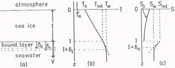
Fig. 1. Schematic illustration of a model of growing sea ice. Temperature profile (b) and salinity profile (c).
-
1) Atmosphere, ice and water are horizontally homogeneous so that temperature T and salinity S depend on only vertical direction z (Figure 1).
-
2) The temperature profile in ice is governed by the solution of the equation of heat conduction under steady state conditions, i e
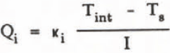
where κi is the thermal conductivity, p the density and c the specific heat of sea ice. Therefore, T is linearly proportional to z;(1) where TB is the temperature of the upper surface of ice (z = 0), Tint the temperature of the ice/water interface (z -I), iè the lower surface of ice, and I the thickness of ice. However, the change in temperature at a fixed position in ice is taken into account through an increase in I with time. Such a solution is called a quasi-steady state solution. In the Equation 1, internal heating due to incoming short-wave radition is neglected. The conductive heat flux through ice is given by(2)(3)
 -
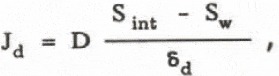
3) A diffusion boundary layer with a thickness δd is formed in the seawater near the tower surface of ice (Figure la and lc). Since only a part of the salt molecules in water can be incorporated into ice, the remainder is rejected at the growing lower surface of ice and the salinity sint.in water adjacent to the lower surface (z = I) becomes larger than the salinity Sw of water at Z » I. The rejected salt molecules are carried away by diffusion in the boundary layer with a flux
where D is the diffusion constant of salt molecules in water.(4) -
4) The salinity S; of ice determined by incorporation kinetics at Z - I is proportional to Sint:
where k* is the so-called distribution coefficient at the cellular ice/water interface (Weeks and Lofgren 1967).(5) -
5) The temperature ?int at z = I is equal to the freezing temperature which is determined by the salinity Sint:
where α is the slope of the liquidus line of the phase diagram of a water-salt system. Therefore, Tint is lower than Tw by(6)(7) -
6) A thermal boundary layer with a thickness δt exists in water near the lower surface of ice (Figure la and lb). Therefore, the conductive heat flux from water to ice is given by
where κw is the thermal conductivity of seawater.(8) -
7) There are several incoming and outgoing heat fluxes at the upper surface ( z = 0) of ice. Incoming fluxes include long-wave radiation Qy from the atmosphere, short-wave radiation Qs in and conductive heat Qithrough the ice towards the upper surface. Outgoing fluxes consist of long-wave radiation Ql out, sensible heat Qsen and latent heat of sublimation Qsub.
where ε is the long-wave emmisivity, σ the Stefan-Boltzmann constant and Ta the temperature of the atmosphere.(9)(10)where Lsp is the latent heat of sublimation in J/m3 , s the humidity, pa(T) the saturation vapour pressure of ice at T in Pa and (ape/aT)T the temperature coefficient of the saturation vapour pressure at T given by the Clausius-Clapeyron equation. Equation 11 was derived from the empirical relation obtained by Ono and others (1980).(11)


DETERMINATION OF THE GROWTH OF SEA ICE
Heal balance at the lower surface of ice
The process which directly controls the growth rate V of sea ice is the conduction process of the latent heat of freezing. From the heat budget equation at z = I, we obtain an expression

Equilibrium condition for Tint
As shown in Equation 6, T , is assumed to be equal to the equilibrium freezing temperature corresponding to the salinity Sint which is determined by the following mass conservation conditions of salt molecules at z = I.
Mass balance of salt molecules at the lower surface of ice
Since only a portion of the salt molecules in water is incorporated into ice at z = I (see Equation 5), the salt molecules are rejected there by amount of V(Sint - Si) = V(l - k*)Sint per unit time and unit area. The quantity should be equal to the diffusion flux Jd given by Equation 4 under steady state conditions:

Therefore, we obtain a relation between Sint and V
Heat balance at the upper surface of ice
The temperature Ts is determined by the balance equation of the heat fluxes at z = 0 mentioned in section 2:


A = 23.4 W/m2K and B = 60.7 W/m2, if we assign Ta =253 k E= 1, σ = 5.67x10⁻⁸ W/m2K4, Ua = 5 m/s, Lsp = 2.6xl09 J/m3, (βρ./3?)T = 10.4 Pa/K, Pe(Ta) = l.03xIO2 Pa, s = 0.8, Ql = 1.76xl02 W/m2 and Qs in = 0.
From Equation 16 one can see that Ts = Ta for A-«»→∞ and Ts = Tint for ki→∞. These results are plausible.
It should be noted that Tint and Ts which control the growth rate V (Equation 12) themselves depend on V (see Equations 6, 14 and 16).
Growth rate
By solving Equations 12, 6, 14 and 16 self-consistently, we can obtain an expression for the growth rate V as a function of temperature Ta of the atmosphere and T of sea water:


The obtained growth rate includes the physical quantities relevant to the processes of freezing, conduction of the latent heat of freezing, incorporation of salt into ice, diffusion of salt molecules, incoming and outgoing radiation, transport of sensible heat and latent heat of sublimation as described above.
DISCUSSION
Growth rate
Using Equations 19, 20, 16’ and 21, let us discuss the influence of the environmental conditions on the growth rate of sea ice.
In the most extreme case that SW=0 and A→∞ ,Tint =Tw = 273 K, Ts - Ta and = 1. Therefore, we obtain the simplest Stefan equation V(0) from Equation 19:

If Sw > 0 and D →∞ >, Sint is equal to Sw because of infinite rate of diffusion of rejected salt molecules, then Tint= Tw and ζ = 1. In this case, the growth rate is expressed as

In the general case that Sw > 0 and D is finite, Sint> Sw because of finite rate of diffusion of salt molecules, consequently TintTw and <1. Therefore, the growth rate V in the general case given by Equation 19 is smaller than v(1) by a factor of ζ. It should be noted that 1/ corresponds to the interface resistance to the growth due to the coupling processes of material and heat transports in the diffusion and thermal boundary layers (Figure 1).
With increasing Sw the growth rate decreases because of a decrease in v(1) and ζ in this model. The first effect is due to a decrease in Tw with Sw. On the other hand, the second effect is rather complicated. Since an increase in Sw makes the diffusion of salt molecules slower (the right side of Equation 13) and consequently raises Sint (Equation 14), Tint falls with Sw (Equation 6). Therefore, V decreases with Sw (Equation 12). A decrease in f, with Sw represents this effect.
In this paper, we assume that the thickness d of diffusion boundary layer is given. The value of d/D reported by Weeks and Lofgren (1967) is 5.09 x 10⁵ s/m and that by Nakawo and Sinha (1981) is 4.2 x 10⁶ s/m. If D is assumed to be 1 x 10⁻⁹ m2/s, d » 0.51 mm in the former case and d = 4.2 mm in the latter case. The thickness d is expected to decrease with flow velocity Uw of water, since the thickness of velocity boundary layer decreases with Uw. A decrease in 6d leads to an increase in ζ or V because of faster diffusion of salt molecules. However, the influence of Uw on V through the thickness 6, of thermal boundary layer is different. With increasing Uw, t, may also decrease. And Ç decreases with decreasing t (Equation 21), since the heat flux Qw from water to ice increases with decreasing t (the second term of the right side in Equation 12).
The dependence of the growth rate on the thickness I of sea ice is shown in Table 1. The numerical values used for calculation are as follows: T, = 253 K, K = 2.26 W/m K, KW = 0.52 W/m K, α = 0.055 K/°/°°, SW = 32.9°/°°, LfP = 3.08 x 10⁸ J/m3, k* = 0.12, δd/D - 4.2 x 1°6 s/m, δt, = 2 x 10⁻²m, A = 23.4 W/m2 K and B = 60.7 W/m2. With increasing I, V(1) decreases because of a decrease in conductive heat flux in ice. On the other hand, ζ slightly increases with I, since the flux of rejected salt moelcules decreases with decreasing growth rate (see the left side of Equation 13). However, this is a secondary effect, so that V=V(1) decreases with I.
Effective distribution coefficient keff
From Equations 5 and 14, we obtain the so-called effective distribution coefficient keff = Si/Sw of salt molecules.
where V is given by Equation 19. The salinity Si in ice is expected to decrease with z (Figure lc), since the growth rate V in Equation 22 decreases with I. The Equation 22 coincides with the expression for keff derived by Weeks and Lofgren (1967), if dV/D « 1.
Heat flux Qw from water to ice
Using Equations 8’ and 14, the heat flux Qw from water to ice is given by
This equation means that the growth rate V feeds back to the heat flux Qw which controls V because of coupling of salt diffusion in the diffusion boundary layer and heat conduction in the thermal boundary layer.
Table 1. The Dependence on the Thickness I of Sea Ice of the Growth Rate V and the Heat Flux Qw from Water to Ice.

As shown in Table 1, Qw decreases with the thickness I of sea ice, even if the environmental conditions are kept constant. An increase in I leads to a decrease in Sint (Equation 14), since V decreases with I. Therefore, Qw falls with I (Equations 8’ and 14). On calculation, we assumed d/t - 0.2 and D = 1 x 10⁻⁹ m2/s.
ACKNOWLEDGEMENT
The author is indebted to Professor N Ono and Dr N Ishikawa for helpful discussions.


