1. Introduction
The texture of snow is of critical importance to snow properties (Reference EugsterEugster, 1950; IASH Commission of Snow and Ice, 1954; Reference ColbeckColbeck and others, 1990; Reference Schneebeli, Pielmeier and JohnsonSchneebeli and others, 1999). Increasingly, the more precise numerical simulation of snow (Reference Brun, David, Sudul and BrunotBrun and others, 1992; Reference Lehning, Bartelt, Brown, Fierz and SatyawaliLehning and others, 2002; Reference Singh, Satyawali, Srivastava, Sethi, Ganju and GanjuSingh and others, 2004) is limited by the precision of observation. Almost all snow-pit measurements are subject to inaccuracy due to subjectivity associated with human perception. In the field, snow texture is recorded in terms of grain size and grain shape using visual techniques which can be highly subjective. In the cold laboratory, sections of snow samples are taken to obtain grain size and distinguish snow classes. The latter approach, while much more quantitative, is generally not chosen, due to time constraints and the difficulty of bringing field samples to the cold room. Due to its subjective nature, traditional classification shows a larger scatter of data. The consequence is an improper comparison of snow class between the datasets of different observers.
Reference Schneebeli, Pielmeier and JohnsonSchneebeli and others (1999) modelled texture index (TI) for snow from the data of a high-resolution snow penetrometer, the SnowMicroPen (SMP; J.B. Johnson and M. Schneebeli. 1998. Snow strength penetrometer. US Patent 5831161). The TI is defined as the ratio of the mean grain size to the volumetric density, which Reference Schneebeli, Pielmeier and JohnsonSchneebeli and others (1999) showed could be estimated from the coefficient of variance (CV) of the SMP signal. They were able to partly correlate weak layers with the textural information as obtained from the penetration force data of SMP profiles (the full-length signal of snowpack). The CV is also used to quantify changes in texture (Reference PielmeierPielmeier, 2003; Reference Lutz, Birkeland, Kronholm, Hansen and AspinallLutz and others, 2007). Reference Pielmeier, Schweizer, Stucki and ElderPielmeier and others (2005) and Reference Pielmeier and SchweizerPielmeier and Schweizer (2007) compared SMP profile data with manual stability test scores and found them fairly reliable for predicting stability. Snow strength was also modelled using a micromechanical theory (Reference Johnson and SchneebeliJohnson and Schneebeli, 1999), but results were only qualitatively compared to descriptions of snow classes. Later, a statistically based micromechanical theory of cone penetration in granular material was developed by Reference JohnsonJohnson (2003), which takes into account the effects of cone geometry, material compaction and the dimension and strength of the microstructural elements that form the granular material. Johnson showed the dependence of cone penetration resistance on cone half-angle and concluded that the micromechanical theory may provide a means to directly determine geotechnical properties of granular materials. Reference Satyawali, Schneebeli, Pielmeier, Stucki and SinghSatyawali and others (2009) characterized Alpine snow based on a hierarchical look-up table supported by a database of classified SMP profiles. The approach was found to be useful for detecting snow class with reasonable accuracy. Reference Matzl and SchneebeliMatzl and Schneebeli (2006) used infrared photography to estimate optical equivalent snow grain size directly from the snow pit. Reference Dadic, Schneebeli, Lehning, Hutterli and OhmuraDadic and others (2008) used SMP profile data to capture more detailed information on snowpack, and found that high-resolution data were necessary to accurately model near-surface temperatures in polar snow.
None of these methods provides satisfactory results for snow characterization in an objective manner. The current method of snow characterization using SMP measurements is based on simple moments, so a new method is developed in the present work to improve snow classification using geostatistics. The method is based on the spatial measures of snow estimated from the semivariogram (SV). It is recognized that combining simple moments and spatial measures will improve snow classification.
Several recent studies on snow, which are based on the application of geostatistics (Reference Webster and OliverWebster and Oliver, 2001), estimate the SV (Reference PielmeierPielmeier, 2003; Reference Birkeland, Kronholm, Logan and GanjuBirkeland and others, 2004; Reference KronholmKronholm, 2004; Reference Kronholm, Schneebeli and SchweizerKronholm and others, 2004; Reference Lutz, Birkeland, Kronholm, Hansen and AspinallLutz and others, 2007) for quantifying the spatial variability of selected snow layers. Reference Lutz, Birkeland, Kronholm, Hansen and AspinallLutz and others (2007) found a microscale correlation length of 80 μm within a weak layer. Using a micromechanical model (Reference Johnson and SchneebeliJohnson and Schneebeli, 1999; Reference JohnsonJohnson, 2003), Reference LutzLutz (2009) estimated micromechanical parameters of weak interfaces from the SMP data and found variability over time and space. Using compression test results and the autocorrelation function on SMP penetration resistance, Van Herwijnen and others (in press) were able to resolve layer boundaries and the failure layers. Estimating the correlation length for an entire snow class could be useful for future research on snow classification.
Natural phenomena such as earthquake distribution, biological systems, geological structures and geophysical properties are mainly described as self-affine fractals by many researchers (Reference KorvinKorvin, 1992; Reference De Santis, Fedi and QuartaDe Santis and others, 1997; Reference TurcotteTurcotte, 1997; Reference DimriDimri, 2000; Reference Bansal and DimriBansal and Dimri, 2005; Reference Chamoli, Bansal and DimriChamoli, and others, 2007). Reference CarrCarr (1995) used the SV to estimate the fractal dimension (FD) of a stochastic fractal. Reference Mela and LouieMela and Louie (2001) used the SV to obtain the correlation length and FD of seismic data. In general, as measurement scale becomes smaller the corresponding measured property shows fractal behaviour (Reference FederFeder, 1988; Reference CrossCross, 1997; Reference Wallace, Morris and HowarthWallace and others, 2004). In snow, since ice and pores are randomly distributed even for a homogeneous snow, the high-resolution SMP data of snow resistance exhibit it in the form of varying penetration force. Reference Deems, Fassnacht and ElderDeems and others (2006) observed the spatial distribution of snow depth at horizontal scales from 1 to 1000 m using variogram fractal analysis and found two distinct FDs for short- and long-range correlation.
In the present work, we show the range parameter (hereafter correlation length (CL)) of major snow classes as estimated from the SV. SMP measurements were also taken in the ground-parallel direction in the snowpack while supported on the level ground. CL was obtained along this direction, and a ratio of CL in the ground-parallel and ground-perpendicular direction is used to estimate directional anisotropy. An attempt was also made to show the relation between TI and CL. The SV method is also used to estimate the FD of the penetration force data from the log–log plot of the SV (e.g. Reference Zhang, Person, Paola, Gable, Wen and DavisZhang and others, 2005), and the dependence of the FD on snow class is demonstrated.
2. Methods
2.1. Experimental site and data collection
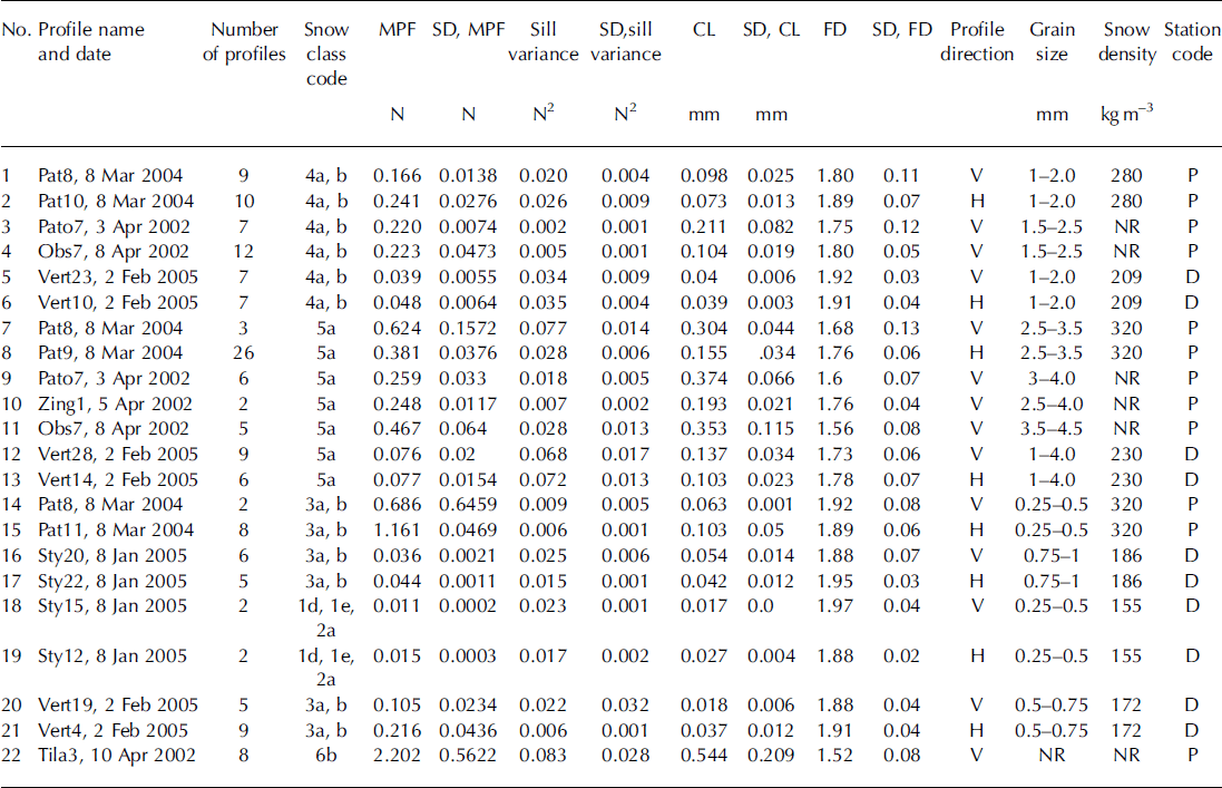
In order to estimate the spatial scales for different snow classes from the field, precise measurement of the snow layers (in SMP profile and hand profile) is very important. The present study is based on measurements made for snow at Patsio, Himachal Pradesh, India (32.75° N, 77.25° E; 3800 ma.s.l.), and at Davos, Switzerland (46.48° N, 9.49° E; 1560 m a.s.l.). The SMP profiles and manual snow-pit measurements were taken during mid-winter to late winter in order to ensure that major snow classes were captured. These measurements were done for ground-parallel and ground-perpendicular directions along with manual snow-pit profiles. The details of each SMP profile, with date, snow class, snow density and profile direction, are given in Table 1. Measurements were made on 7 days (5 days at Patsio during 2001/02 and 2003/04, and 2 days at Davos during 2004/05), resulting in a total of 98 SMP profiles from Patsio and 58 SMP profiles from Davos (Table 1, column 2) available for analysis.
Table 1. Mean spatial data obtained for various snow classes over 20 mm distance. The snow class codes are according to Reference ColbeckColbeck and others (1990). SD: standard deviation; V: ground-perpendicular, H: ground-parallel, NR: not recorded; P: Patsio; D: Davos
The SMP records penetration force data at 4 mm intervals. Such closely spaced data allowed geostatistics to be applied even for a SMP profile segment of <20 mm. In the present work, a 20mm SMP profile segment was selected for analysis of all the snow classes. Precise matching of SMP profile segments with the snow-pit profile is very important. A 20 mm profile segment for a particular snow class was selected visually by matching the snow-pit profile with the SMP profile. Thin snow layers were not considered, as they could be visually missed in the SMP profile. Only thick prominent snow layers from both the profiles (SMP and manual) were considered for this analysis. In this way, manual error in aligning the SMP and the snow-pit profiles was minimized.
2.2. Performance of different SMPs
In the present study, four different SMPs were used to take the snow profile. The semivariance of the air signal was analysed for all the SMPs as in Reference LutzLutz (2009). The air signal was recorded before the sensor tip entered the snowpack. It was taken from a 10 mm segment and plotted for 0.02 mm lag distance for all the SMPs (Fig. 1). The semivariance shows no spatial correlation, but a pure nugget effect. For three of the SMPs (SMP1, SMP2, SMP3) the semivariance was found to be around 10−6 N2, and for one (SMP4) about 10−5 N2. SMP4 had different, coarser, gear spacing than the other SMPs. However, the variance is very small compared to the typical penetration resistance of the snow investigated here. In this study, the data were not examined for poor-quality signal. In addition, we did not use a micromechanical model (Reference Johnson and SchneebeliJohnson and Schneebeli, 1999) which can be sensitive to instrument noise (Reference LutzLutz, 2009).
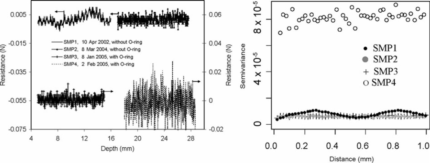
Fig. 1. Comparison of air signal for different SMPs used in the present work (a) with semivariance analysis (b).
2.3. Estimation of semivariogram
The SV relates the variance in values of an attribute at pairs of sample points to separation distance between the points of a given pair. It is therefore a measure of spatial dependence of a variable over some distance. The SV can be used to determine the scaling properties of self-affine series (Reference Oliver and WebsterOliver and Webster, 1986), which are related to lag distance (h) as follows (Reference CressieCressie, 1993):

γ(h) is defined as the experimental SV or sample SV, i.e. one based on the sampled dataset, (N – h) is the number of pairs at lag distance h, and Y(xi) is the parameter value at position i. Y(h) is then plotted against the lag distance between the initial point and the compared points. The plot typically results in a curve where SV value increases with distance to a maximum, and then levels off if the distance between measurement points exceeds the distance at which spatial structure exists. A continuous process without spatial dependence will result in a horizontal line beyond the CL, called sill variance. The lag distance where the model SV reaches the sill variance is called CL. The CL is the maximum distance over which there is spatial autocorrelation. The nugget variance is caused mainly by variance over distances less than the sampling interval and also due to measurement error.
For calculation of CL, the SVs were plotted only up to one-quarter of the extent of data because the SV is not reliable for the lag distance beyond this limit (Reference Oliver and WebsterOliver and Webster, 1986). According to Pfeiffer (1996), ‘Estimates of the SV are considered to be more robust to departures from stationarity represented as a general trend in the spatial process’. Reference Jaksa, Kaggwa, Brooker, Li and LoJaksa and others (1993) showed that sampling at close spacing is very important in estimating SV, as the larger-spaced sample data reach the sill variance at the very beginning. It is therefore visualized that SMP data can be used in estimating SV, as they capture high-resolution information at equally spaced intervals.
2.4. Processing of SMP profile data
For each snow class, a fixed segment 20 mm long is selected from the SMP profile for the purpose of estimating the SV. It was first ascertained that SMP data belong to a log-normal distribution. This was done by applying a log transformation to the SMP profile segment. The distribution was checked by a quantile–quantile (QQ) plot, which shows a straight line for normally distributed data.
Similar to the autocorrelation function of random variables, the SV requires stationary data, which means that it should depend only on the separation distance and not on the locality of the pairs. As a result, if a drift or trend exists in the data, it must first be removed. Reference DavisDavis (1986) showed that if the trend is subtracted from the variables, the residuals themselves will be a variable with a local mean value of zero. An example of a typical trended penetration-force record for a rounded-grain snow layer is shown in Figure 2a. The QQ plot (Fig. 2b) shows that these data are far from the normal distribution and require treatment to make them normal before estimating the SV. Figure 2c shows the QQ plot after a log transformation is applied. The SV (Fig. 2d and e) is shown before and after the linear trend is removed from the data using statistical software ‘R’ (Reference Ribeiro and DiggleRibeiro and Diggle, 2001).
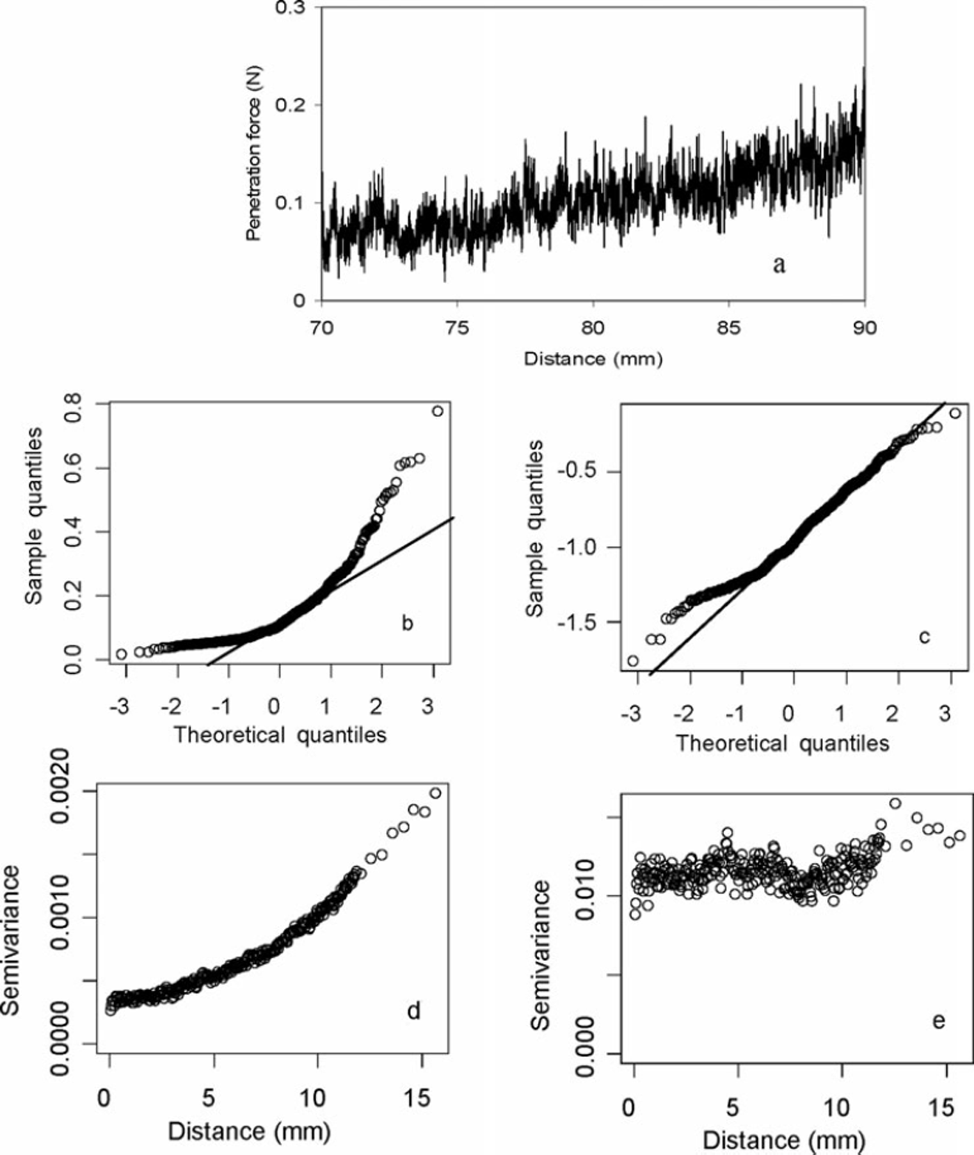
Fig. 2. (a) Signal from a segment of 20 mm SMP profile of rounded-grain snow. (b) QQ plot of sample data. (c) QQ plot after log transformation. (d) SV of trended data. (e) SV of detrended data.
A total of 156 samples of the SV were studied for all the snow classes. The fitting of the SV was done by the ordinary least-squares method (Reference CressieCressie, 1993, p. 94) implemented in the R function ‘VARIOFIT’. At large lag distances, the number of point pairs in each lag distance becomes relatively small. This method ensures that outliers in the data are handled automatically by giving them low weight (this was done by taking more than 200 data pairs for each lag distance) in the calculation of the SV. The sample SV is modelled with an exponential SV model plus a zero nugget (Equation (2)) as:
where c + c 0 is sill variance, a is CL and c 0 is nugget. These parameters are used to describe the SV.
2.5. Estimation of correlation length and texture index
To estimate CL for a full-depth SMP profile, the SV was first obtained for a 5 mm profile length, starting from top to bottom continuously. Since there were chances to capture more than two homogeneous snow layers for a 20mm profile length, SV was only estimated for a 5 mm profile length to reduce error. Estimates of the SV for segments less than 5 mm were not considered because of the cone tip size of the SMP, which is 4.3 mm (Reference Lutz, Birkeland, Kronholm, Hansen and AspinallLutz and others, 2007). The CL was than compared with the TI and plotted against snow depth as shown later.
2.6. Estimation of fractal dimension
The following relationship is used to obtain FD by utilizing the slope of a log–log plot of the SV (Reference CarrCarr, 1995):
where S is the slope of the straight line fitted to the linear portion of a log–log plot of the SV. The linear portion was chosen for the data up to the CL distance.
3. Results and Discussion
After analyzing the SV, it was found that CL, sill variance and nugget from the fitted models for each class varied slightly. For most cases, the exponential model (Equation (2)) provided the best visual fit. To ensure that the parameters of the model SV were directly comparable, the best-fit model (exponential) was used for the analyses. This seems a reasonable choice because the results of kriging are much the same for any reasonable choice of SV model (Reference Webster and OliverWebster and Oliver, 2001). The results of the statistical analysis are given in Table 1 which shows the mean penetration force (MPF) averaged over 1 mm profile length, sill variance, CL and FD with their standard deviations. Snow density and grain size as measured during pit profiles are also given. Himalayan snow had higher average density (307±20 kgm−3) than Alpine snow (190 ± 2 8 kgm−3).
3.1. Sill variance
Rounded-grain snow showed higher sill variance in the ground-perpendicular direction, and faceted-grain snow in the ground-parallel direction (see Table 1). The sill variance of depth-hoar snow (profile Nos. 7 and 8) for Himalayan snow is higher than for Alpine snow (profile Nos. 12 and 13), but a significant difference was not observed.
Figure 3a-d show the sample SV obtained for faceted snow, depth hoar, rounded-grain snow and new snow respectively. The model SV (exponential) is also plotted for all the snow classes. Sill variance is highest for depth hoar and lowest for rounded-grain snow. Cyclic behaviour of the SV was also noticed for depth-hoar snow at small distances.
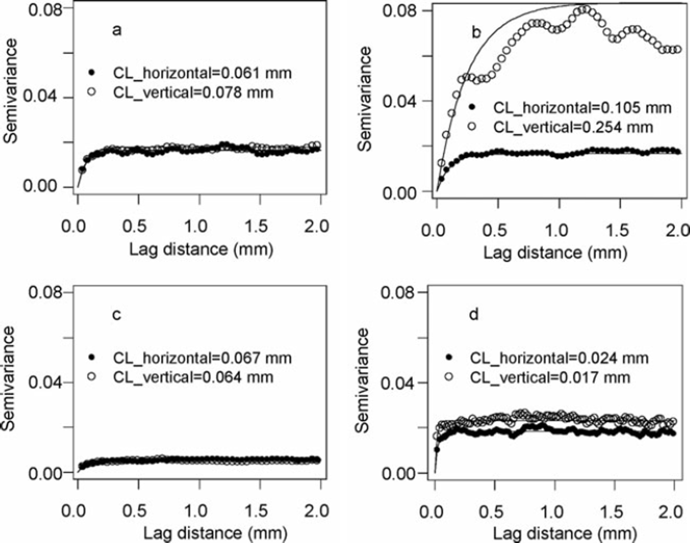
Fig. 3. Sample and modelled (exponential) SV for (a) faceted snow, (b) depth hoar, (c) rounded grain and (d) new snow. (Prefix CL_ is correlation length.)
3.2. Mean penetration force, correlation length and anisotropy
The MPF for all the measured snow classes was analysed. As expected, it was found to be highest for melt–freeze snow and lowest for new snow (Table 1). Depth-hoar and faceted-grain snow show low MPF values, with faceted-grain snow showing the lower values. Rounded-grain snow shows intermediate MPF values, with large scatter due to varying snow density and bonding (not measured in the present work). From Table 1 (profile Nos. 14–21), most of the layer analysis for rounded-grain snow suggests that snow resistance is greater in the ground-parallel than in the ground-perpendicular direction.
As the SV was estimated in both directions, the ratio of the directional CL (also defined as anisotropy) is further utilized in the interpretation of the data. Figure 3a–d show the SV obtained for different snow classes in different directions. Shortly after it is deposited, as snow is relatively new or slightly metamorphosed, the CL is greater in the ground-parallel direction (Fig. 3d). For new snow, the ratio of the CL (ground-parallel to ground-perpendicular direction) as averaged for the present data is 1.59 (Table 1). It is logical that new snow crystals tend to descend with the basal plane parallel to the horizontal plane. Once snow is settled, the metamorphic process alters the grain shape into a rounded or angular shape depending on temperatures and temperature gradients. This results in varying CL values for different snow classes. The anisotropy therefore changes with the metamorphic processes. For rounded-grain snow, the ratio was 1.63, and for faceted-grain snow it was 0.74, i.e. less than 1. This means that snow textures dominate in the ground-perpendicular direction for this snow. For well-developed depth-hoar snow, the ratio was found to be even less (0.51). This implies that more alignment of snow texture takes place in the ground-perpendicular direction as snow changes shape from new snow to depth hoar. This analysis gives an idea how snow texture develops with time as snow metamorphism progresses. However, it is worth mentioning that, due to the tip geometry of the SMP, it is not known whether the dimensions are physically related only to the snow structure, or to the size and geometry of the tip as well.
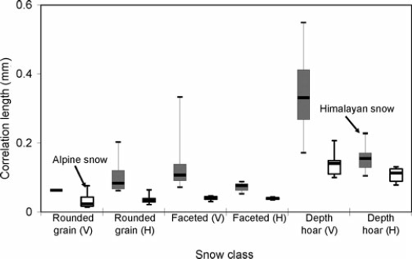
Figures 4 and 5 show the MPF and CL respectively. Boxes show the interquartile range from the first to third quartile, with a horizontal line showing the median. Himalayan snow (grey boxes) shows higher values of MPF and CL. MPF is found more in the ground-parallel direction (H) than the ground-perpendicular direction (V) for both Himalayan and Alpine snow (white boxes), except for Himalayan depth hoar. Among all snow classes, Himalayan rounded-grain snow shows higher MPF in the ground-parallel direction. The CL is higher in the ground-perpendicular direction than the ground-parallel direction for the same class of snow. Depth hoar shows the highest value of CL in the ground-perpendicular direction.
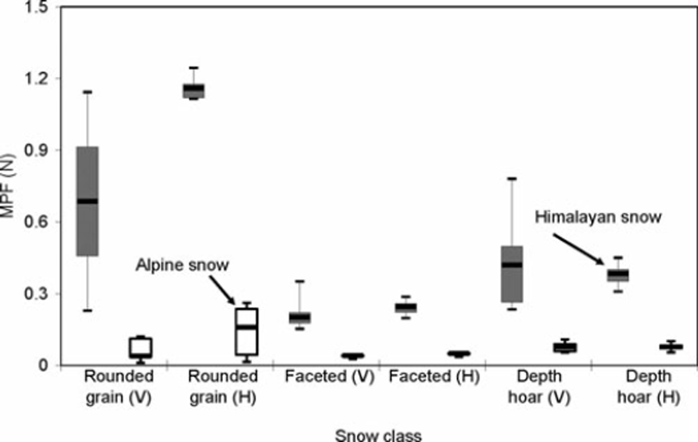
Fig. 4. Box plot of mean penetration force (MPF). Himalayan snow is shown in shaded gray and alpine snow shown with white box plots. The data are from a sample size of 156 as shown in Table 1. Snow profiling in the ground-parallel and ground-perpendicular directions is represented by H and V respectively.
3.3. Comparison of correlation length with texture index
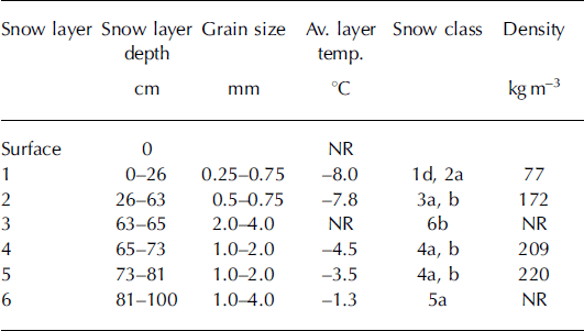
The CL for a full-depth SMP profile for Himalayan snow (using SMP2) and for Alpine snow (using SMP4) is plotted along with the penetration force and TI (Figs 6 and 7). Details of the hand profile are given in Tables 2 and 3 respectively. The CL in both profiles provides a satisfactory comparison with the TI, at least visually, showing the potential of this approach. Because the TI correlates well to the grain size (Reference Schneebeli, Pielmeier and JohnsonSchneebeli and others, 1999), CL must also be correlated to grain size. The correlation is not obtained between CL and TI, as these parameters are estimated for varying profile length.
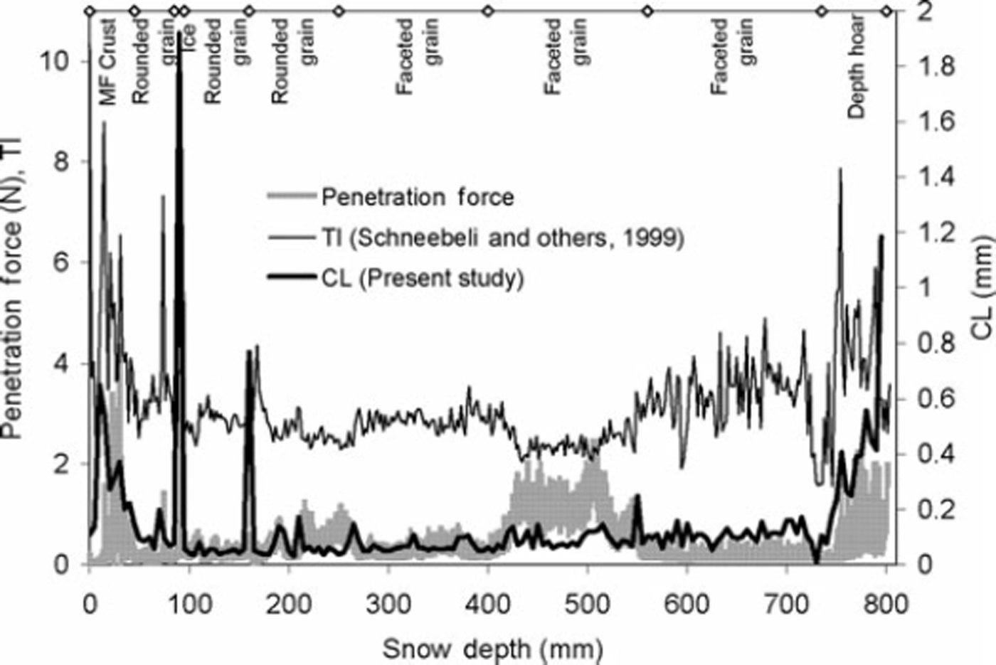
Fig. 6. Comparison of penetration force and texture index (TI) with CL for Himalayan snowpack. Observed snow class is also shown. Details of hand profile given (Table 2). (⋄: layer interface marker.)
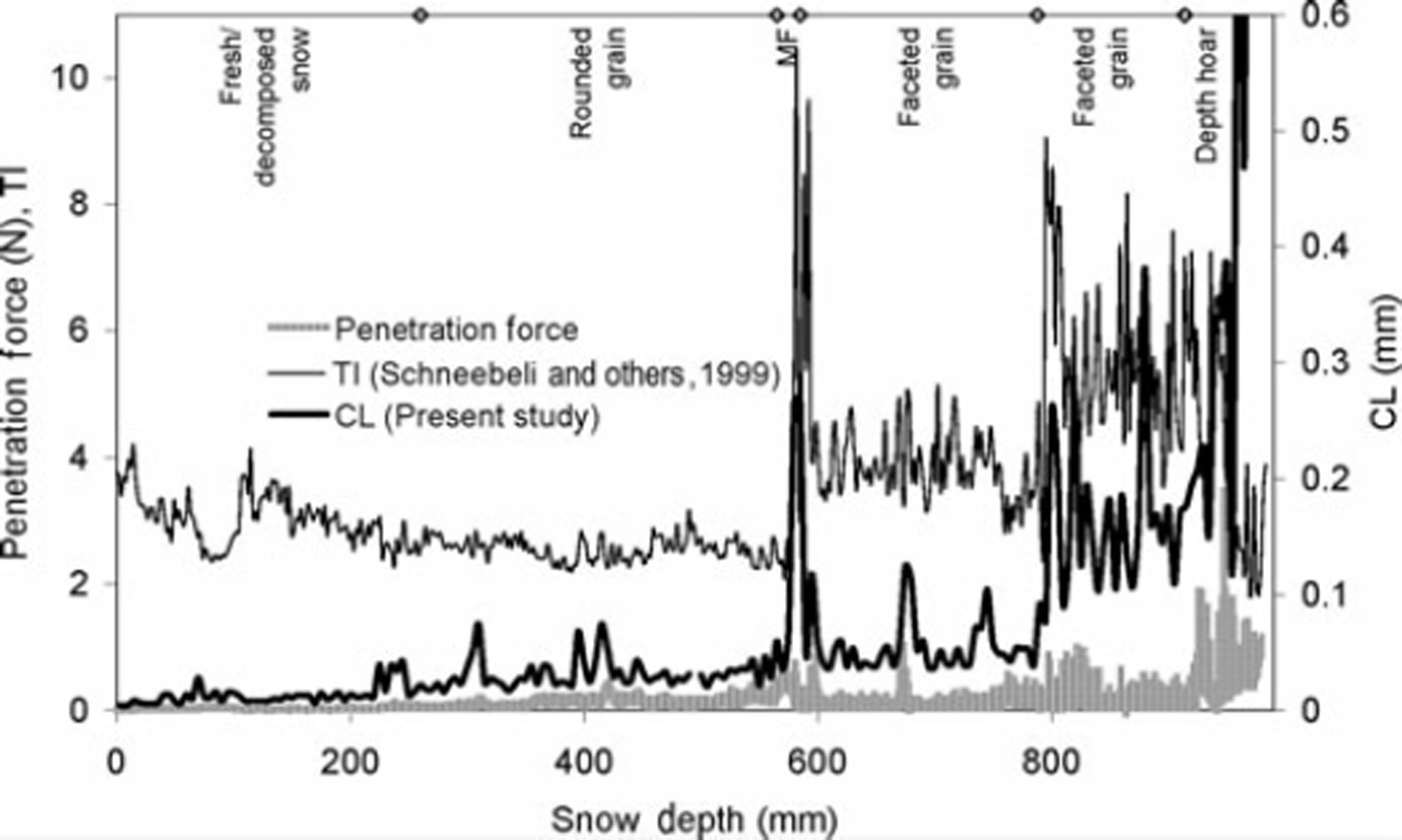
Fig. 7. Comparison of penetration force and TI with CL for Alpine snowpack Observed snow class is also shown. Details of hand profile given (Table 3). (⋄: layer interface marker.)
Table 2. Details of hand profile for Himalayan snowpack taken on 8 March 2004. The snow class codes are according to Reference ColbeckColbeck and others (1990). NR: not recorded
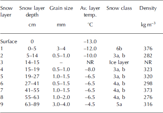
Table 3. Details of hand profile for Alpine snowpack taken on 2 February 2005. The snow class codes are according to Reference ColbeckColbeck and others (1990). NR: not recorded
3.4. Fractal dimension
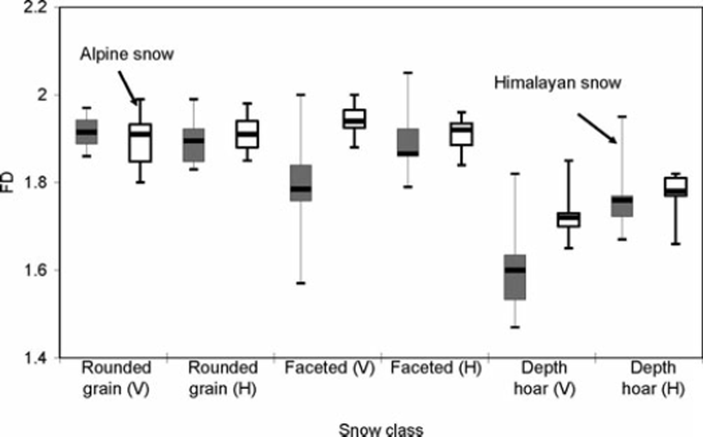
The FD can be estimated from the SV (Reference CarrCarr, 1995) provided the data are sampled at equal intervals to indicate the similarity of the features understudy. The evenly spaced data of the SMP are therefore well suited to such analysis. Figure 8 shows an example of the SV plotted on a log-log scale for four major snow classes. A linear regression was obtained for all the data below the CL distance, which shows a linear portion on a log-log scale. Once the slope is estimated, the FD is calculated using Equation (3). FDs in the ground-parallel and ground-perpendicular directions show no definite correlation (Table 1; Fig. 9). The average FD for Himalayan and Alpine snow, however, varies according to snow class, being highest for rounded-grain snow and lowest for melt–freeze snow (FDRounded_grain = 1.91 ± 0.035, FDFaceted_grain = 1.85 ± 0.07, FDDepth_hoar = 1.7 ± 0.09 and FDMelt–freeze = 1.52 ± 0.08).
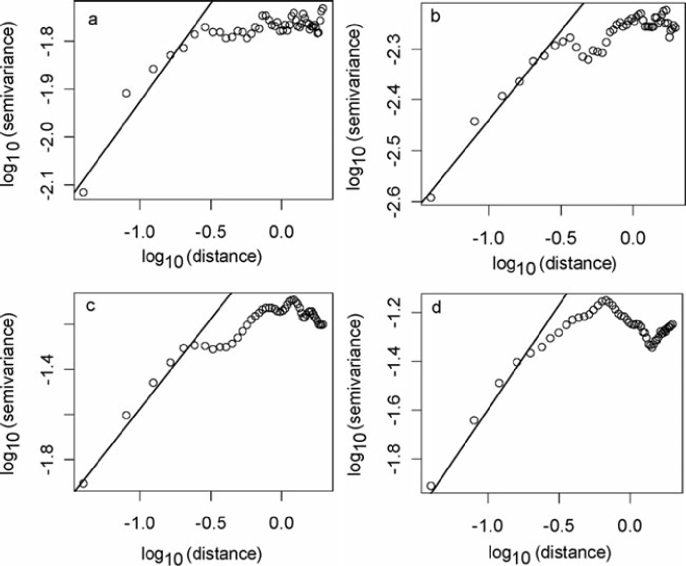
Fig. 8. Log–log plots of SV: (a) faceted snow, (b) rounded-grain snow, (c) depth hoar and (d) melt–freeze. A linear regression line (considering first six points) is drawn to find the slope.
The directional distribution of the FD for Himalayan and Alpine snow is shown in Figure 9. Himalayan snow shows lower FD values than Alpine snow for all the snow classes. Depth-hoar snow shows the smallest values of FD in the ground-perpendicular direction for both Himalayan and Alpine snow.
The variation of CL with FD is shown in Figure 10 along with uncertainty in the measurement. It shows a better grouping of data, as different datasets lie in a particular range. In each case, CL is found to decrease with increasing FD values. Small FD values correspond to coarser grains, and larger values to finer particles.
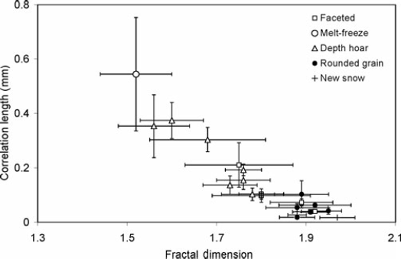
Fig. 10. Variation of CL with FD. Standard mean error bars are shown.
4. Conclusion
One-dimensional semivariance analysis helped in the description and modelling of snow characterization from penetration force data of SMP profiles obtained through a high-resolution penetrometer (J.B. Johnson and M. Schneebeli, US Patent 5831161). The SV is plotted to estimate the spatial scales of various snow classes. The range parameter obtained from the SV is interpreted as the CL. The SV extracted from the SMP profiles is found to be useful for interpreting spatial scales. For all snow classes, CL is generally found to increase with snow density. However, to validate this fact, sufficient data covering a wider range (over both time and space) will be required. This was beyond the scope of the present work. The Patsio and Davos sites were considered to show the potential of this method for acceptable characterization of identical snow even from different locations.
Directional SV obtained for major snow classes can be used to interpret the snow property. The spatial length shifts from a maximum in the ground-parallel to ground-perpendicular direction with an increasing degree of temperature gradient metamorphism. The study, however, lacks the data of average temperature gradient and temperature for validation. The FD of penetration force was obtained from the log–log plot of the SV, and was found to be useful for characterization of snow.
The technique of geostatistics is utilized to explain the issue of randomness and continuity of spatial data by using the SV. Higher spatial continuity, observed in melt–freeze and depth-hoar signals, is characterized by smaller values of FD; less spatial continuity, observed in rounded-grain snow, is distinguished by larger FD. The results indicate that spatial scales are important parameters for characterizing snow class. The sampling resolution (4 μm) seems to be sufficient to explain the small-scale variations. The method used here is found to be robust because it gives direct information from SMP profiles. The SMP data are analysed for major snow classes due to lack of other snow-class data (surface hoar, wet snow, etc.). The method demonstrated here is, however, a helpful tool in analysing snow profiles objectively. Here we have shown that SV can be used to estimate spatial scales of different snow classes. This is the first effort to use geostatistics in this direction, and further work will help to connect this information with physical and mechanical properties.


