


Impact Statement
Constitutive models relate the strain inside a material body to the stress it evokes. In this work, the excellent flexibility that neural networks offer is exploited to formulate hyperelastic constitutive models, which describe large, reversible deformations. The models are physics-augmented, that is, they fulfill all common mechanical conditions of hyperelasticity by construction. This results in highly flexible yet physically sensible neural network models. These models will be applicable to a wide range of materials, particularly to the representation of microstructured materials, for example, fiber-reinforced composites, metamaterials, textiles, or tissues. By that, computationally more expensive methods can be avoided, thus accelerating the simulation and optimization of engineering components made of microstructured materials.
1. Introduction
Convexity is a convenient property of mathematical functions in many applications. However, it also constrains the function space a model can represent. While for some applications, this constraint is well motivated, it is too restrictive for other use cases. Moreover, there are applications where a function can be motivated to be convex in some of its arguments, while it should not necessarily be convex in the other arguments. The latter is usually the case for hyperelastic material models with parametric dependencies, such as process parameters in 3D printing which influence material properties (Valizadeh et al., Reference Valizadeh, Al Aboud, Dörsam and Weeger2021), or microstructured materials with a parametrized geometry (Fernández et al., Reference Fernández, Fritzen and Weeger2022). In the framework of hyperelasticity, the polyconvexity condition introduced by Ball (Ball, Reference Ball1976, Reference Ball1977) requires the associated energy potentials to be convex functions in several strain measures. However, there is generally no mechanical motivation for a hyperelastic potential to be convex in additional parameters on which it might depend. To reflect this, a modeling framework for parametrized polyconvex hyperelasticity should provide potentials which are convex in the arguments of the polyconvexity condition and can represent more general functional relationships in the additional parameters. Finally, in some cases, further conditions such as monotonicity of the hyperelastic potential in some parameters can be motivated by physical considerations (Valizadeh et al., Reference Valizadeh, Al Aboud, Dörsam and Weeger2021).
In finite elasticity theory, convexity of the energy potential in the primary deformation measure alone (the deformation gradient $ \boldsymbol{F} $
) would be too restrictive. In particular, this would be incompatible with growth and objectivity conditions, and it would not allow to represent certain phenomena such as buckling (Ebbing, Reference Ebbing2010; Section 5.2). Polyconvexity circumvents these problems by formulating energy potentials which are convex in an extended set of arguments, namely the deformation gradient, its cofactor, and its determinant, making this convexity condition compatible with aforementioned physical considerations. When the energy potential is convex in these strain measures (and thus polyconvex) and an additional coercivity condition is fulfilled,Footnote 1 the existence of minimizers of the underlying variational functionals of finite elasticity theory is guaranteed (Kružík and Roubíček, Reference Kružík and Roubíček2019). Indeed, this coercivity condition makes assumptions on the hyperelastic potential which lie far outside a practically relevant deformation range, making the practical relevance of this existence theorem questionable (Klein et al., Reference Klein, Fernández, Martin, Neff and Weeger2022a).
$ \boldsymbol{F} $
) would be too restrictive. In particular, this would be incompatible with growth and objectivity conditions, and it would not allow to represent certain phenomena such as buckling (Ebbing, Reference Ebbing2010; Section 5.2). Polyconvexity circumvents these problems by formulating energy potentials which are convex in an extended set of arguments, namely the deformation gradient, its cofactor, and its determinant, making this convexity condition compatible with aforementioned physical considerations. When the energy potential is convex in these strain measures (and thus polyconvex) and an additional coercivity condition is fulfilled,Footnote 1 the existence of minimizers of the underlying variational functionals of finite elasticity theory is guaranteed (Kružík and Roubíček, Reference Kružík and Roubíček2019). Indeed, this coercivity condition makes assumptions on the hyperelastic potential which lie far outside a practically relevant deformation range, making the practical relevance of this existence theorem questionable (Klein et al., Reference Klein, Fernández, Martin, Neff and Weeger2022a).
Apart from that, from an engineering perspective, polyconvexity is desirable since it implies ellipticity (or rank-one convexity) of hyperelastic potentials (Zee and Sternberg, Reference Zee and Sternberg1983; Neff et al., Reference Neff, Ghiba and Lankeit2015). Ellipticity, in turn, is important for a stable behavior of numerical applications such as the finite element method. Without polyconvexity, the ellipticity of a hyperelastic potential is cumbersome to check, and practically impossible to fulfill by construction. Overall, from an engineering perspective, polyconvexity is desirable since it implies ellipticity, rather than for its significance in existence theorems.
In constitutive modeling, neural networks (NNs) can be applied to represent hyperelastic potentials. These highly flexible models are usually formulated to fulfill mechanical conditions relevant to hyperelasticity, thus combining the extraordinary flexibility that NNs offer with a sound mechanical basis. Such models are precious in fields where highly flexible yet physically sensible models are required, such as the simulation of microstructured materials (Gärtner et al., Reference Gärtner, Fernández and Weeger2021; Kumar and Kochmann, Reference Kumar and Kochmann2022; Kalina et al., Reference Kalina, Linden, Brummund and Kästner2023). Furthermore, including mechanical conditions improves the model generalization (Klein et al., Reference Klein, Ortigosa, Martínez-Frutos and Weeger2022b), allowing for model calibrations with sparse data usually available from real-world experiments (Linka et al., Reference Linka, St. Pierre and Kuhl2023). For the construction of polyconvex potentials, several approaches exist (Chen and Guilleminot, Reference Chen and Guilleminot2022; Klein et al., Reference Klein, Fernández, Martin, Neff and Weeger2022a; Tac et al., Reference Tac, Sahli-Costabal and Tepole2022), where the most noteworthy approaches are based on input-convex neural networks (ICNNs). Proposed by Amos et al. (Reference Amos, Xu and Kolter2017), this special network architecture has not only been successfully applied in the framework of polyconvexity, but is also very attractive in, for example, other physical applications which require convexity (Huang et al., Reference Huang, He, Chem and Reina2021; As’ad and Farhat, Reference As’ad and Farhat2023; Rosenkranz et al., Reference Rosenkranz, Kalina, Brummund and Kästner2023) and convex optimization (Calafiore et al., Reference Calafiore, Gaubert and Corrado2020). Besides this particular choice of network architecture, using invariants as strain measures ensures the fulfillment of several mechanical conditions at once, for example, objectivity and material symmetry. This is well-known from analytical constitutive modeling (Schröder and Neff, Reference Schröder and Neff2003; Ebbing, Reference Ebbing2010) and also commonly applied in NN-based models (Klein et al., Reference Klein, Ortigosa, Martínez-Frutos and Weeger2022b; Kalina et al., Reference Kalina, Linden, Brummund and Kästner2023; Linka and Kuhl, Reference Linka and Kuhl2023; Tac et al., Reference Tac, Linka, Sahli-Costabal, Kuhl and Tepole2023). Finally, by embedding the NN-potential into a larger modeling framework, that is, adding additional analytical terms, all common constitutive conditions of hyperelasticity can be fulfilled by construction, which was at first introduced for compressible material behavior by Linden et al. (Reference Linden, Klein, Kalina, Brummund, Weeger and Kästner2023). Therein, models that fulfill all mechanical conditions by construction are denoted as physics-augmented neural networks (PANNs).
In the literature, also parametrized models were proposed for different applications, both in the analytical (Wu et al., Reference Wu, Zhao, Hamel, Mu, Kuang, Guo and Qi2018; Valizadeh and Weeger, Reference Valizadeh and Weeger2022) and in the NN context (Baldi et al., Reference Baldi, Cranmer, Faucett, Sadowski and Whiteson2016; Shojaee et al., Reference Shojaee, Valizadeh, Klein, Sharifi and Weeger2023). In particular, also parametrized hyperelastic constitutive models were proposed. In Valizadeh et al. (Reference Valizadeh, Al Aboud, Dörsam and Weeger2021), an analytical model is proposed which maps process parameters of a 3D printing process to material properties, by formulating parametrized hyperelastic potentials. In Linka et al. (Reference Linka, Hillgärtner, Abdolazizi, Aydin, Itskov and Cyron2021) and Fernández et al. (Reference Fernández, Fritzen and Weeger2022), parametrized hyperelastic potentials based on NNs are proposed and applied to different homogenized microstructures. However, to the best of the authors’ knowledge, none of the existing parametrized hyperelastic models based on NNs fulfills all constitutive conditions at the same time. In particular, no model fulfills the polyconvexity condition.
To conclude, while parametrized and polyconvex models are well-established in the framework of NN-based constitutive modeling, the link between both still needs to be made. In the present work, this is done by applying partially input convex neural networks (pICNNs) as proposed by Amos et al. (Reference Amos, Xu and Kolter2017). Receiving two sets of input arguments, pICNNs are convex in one while representing arbitrary relationships for the other. With the model proposed in this work being an extension of Linden et al. (Reference Linden, Klein, Kalina, Brummund, Weeger and Kästner2023), all common constitutive conditions of hyperelasticity are fulfilled by construction. In particular, the model fulfills several mechanical conditions by using polyconvex strain invariants as inputs, while the pICNN preserves the polyconvexity of the invariants. Furthermore, growth and normalization terms ensure a physically sensible stress behavior of the model. Two cases are considered, one with an arbitrary functional relationship in the additional parameters and the other being monotonic in the additional parameters. To formulate the functional relationships, three different pICNN architectures with different complexities are applied. The proposed model will be valuable for the representation of microstructured materials. In particular, the model can represent materials with a parametrized microstructure, for example, lattice-metamaterials with varying radii (Fernández et al., Reference Fernández, Fritzen and Weeger2022), fiber-reinforced elastomers where the volume fraction of the fibers might vary (Kalina et al., Reference Kalina, Linden, Brummund and Kästner2023), microstructures with spherical inclusions, where the stiffness of the inclusions might vary (Klein et al., Reference Klein, Ortigosa, Martínez-Frutos and Weeger2022b), or knitted textiles with graded stitch types and knitting parameters (Do et al., Reference Do, Tan, Ramos, Kiendl and Weeger2020). The parametrization allows for both simulation and optimization of such materials, while the polyconvexity of the model ensures a stable behavior of the numerical simulations required for this.
The outline of the manuscript is as follows. In Section 2, the convexity of function compositions is discussed. In Section 3, the fundamentals of parametrized hyperelasticity are briefly introduced, which are then applied to the proposed PANN model in Section 4. The applicability of the parametric architectures is demonstrated by calibrating it to data generated with two differently parametrized analytical potentials in Section 5, followed by the conclusion in Section 6.
1.1. Notation
Throughout this work, scalars, vectors, and second-order tensors are indicated by $ a $
,
$ a $
, $ \boldsymbol{a} $
, and
$ \boldsymbol{a} $
, and $ \boldsymbol{A} $
, respectively. The second-order identity tensor is denoted as
$ \boldsymbol{A} $
, respectively. The second-order identity tensor is denoted as $ \boldsymbol{I} $
. Transpose and inverse are denoted as
$ \boldsymbol{I} $
. Transpose and inverse are denoted as $ {\boldsymbol{A}}^T $
and
$ {\boldsymbol{A}}^T $
and $ {\boldsymbol{A}}^{-1} $
, respectively. Furthermore, trace, determinant, and cofactor are denoted by
$ {\boldsymbol{A}}^{-1} $
, respectively. Furthermore, trace, determinant, and cofactor are denoted by $ \mathrm{tr}\hskip0.35em \boldsymbol{A} $
,
$ \mathrm{tr}\hskip0.35em \boldsymbol{A} $
, $ \det \hskip0.35em \boldsymbol{A} $
, and
$ \det \hskip0.35em \boldsymbol{A} $
, and $ \mathrm{cof}\hskip0.35em \boldsymbol{A}\hskip0.35em := \hskip0.35em \det \left(\boldsymbol{A}\right){\boldsymbol{A}}^{-T} $
. The set of invertible second-order tensors with positive determinant is denoted by
$ \mathrm{cof}\hskip0.35em \boldsymbol{A}\hskip0.35em := \hskip0.35em \det \left(\boldsymbol{A}\right){\boldsymbol{A}}^{-T} $
. The set of invertible second-order tensors with positive determinant is denoted by $ {\mathrm{GL}}^{+}(3)\hskip0.35em := \hskip0.35em \left\{\boldsymbol{X}\in {\mathrm{\mathbb{R}}}^{3\times 3}\hskip0.35em |\hskip0.35em \det \hskip0.35em \boldsymbol{X}>0\right\} $
and the special orthogonal group in
$ {\mathrm{GL}}^{+}(3)\hskip0.35em := \hskip0.35em \left\{\boldsymbol{X}\in {\mathrm{\mathbb{R}}}^{3\times 3}\hskip0.35em |\hskip0.35em \det \hskip0.35em \boldsymbol{X}>0\right\} $
and the special orthogonal group in $ {\mathrm{\mathbb{R}}}^3 $
by
$ {\mathrm{\mathbb{R}}}^3 $
by $ \mathrm{SO}(3)\hskip0.35em := \hskip0.35em \left\{\boldsymbol{X}\in {\mathrm{\mathbb{R}}}^{3\times 3}\hskip0.35em |\hskip0.35em {\boldsymbol{X}}^T\boldsymbol{X}=\boldsymbol{I},\det \hskip0.35em \boldsymbol{X}=1\right\} $
. For the function composition
$ \mathrm{SO}(3)\hskip0.35em := \hskip0.35em \left\{\boldsymbol{X}\in {\mathrm{\mathbb{R}}}^{3\times 3}\hskip0.35em |\hskip0.35em {\boldsymbol{X}}^T\boldsymbol{X}=\boldsymbol{I},\det \hskip0.35em \boldsymbol{X}=1\right\} $
. For the function composition $ f\left(g(x)\right) $
the compact notation
$ f\left(g(x)\right) $
the compact notation $ \left(f\hskip0.35em \circ \hskip0.35em g\right)(x) $
is applied. The Softplus, Sigmoid, and ReLu functions are denoted by
$ \left(f\hskip0.35em \circ \hskip0.35em g\right)(x) $
is applied. The Softplus, Sigmoid, and ReLu functions are denoted by $ s(x)=\ln \left(1+{e}^x\right) $
,
$ s(x)=\ln \left(1+{e}^x\right) $
, $ sm(x)=\frac{1}{1+{e}^{-x}} $
, and
$ sm(x)=\frac{1}{1+{e}^{-x}} $
, and $ {\left[x\right]}_{+}=\max \left(x,0\right) $
, respectively. The element-wise product between vectors is denoted as
$ {\left[x\right]}_{+}=\max \left(x,0\right) $
, respectively. The element-wise product between vectors is denoted as $ \ast $
.
$ \ast $
.
2. Convexity of function compositions
To lay the foundational intuition for constructing convex neural networks, we first consider the univariate function
 $$ f:\mathrm{\mathbb{R}}\to \mathrm{\mathbb{R}},\hskip1em x\hskip0.70em \mapsto \hskip0.70em f(x)\hskip0.35em := \hskip0.35em \left(g\hskip0.35em \circ \hskip0.35em h\right)(x), $$
where $ f $
is composed of two functions
$ f $
is composed of two functions $ g,\hskip0.35em h:\mathrm{\mathbb{R}}\to \mathrm{\mathbb{R}} $
. Given that all of these functions are twice continuously differentiable, convexity of
$ g,\hskip0.35em h:\mathrm{\mathbb{R}}\to \mathrm{\mathbb{R}} $
. Given that all of these functions are twice continuously differentiable, convexity of $ f $
in
$ f $
in $ x $
is equivalent to the nonnegativity of the second derivative
$ x $
is equivalent to the nonnegativity of the second derivative
 $$ {f^{{\prime\prime} }}(x)=\left({g^{{\prime\prime} }}\hskip0.35em \circ \hskip0.35em h\right)(x)\hskip0.35em {h}^{\prime }{(x)}^2+\left({g}^{\prime}\hskip0.35em \circ \hskip0.35em h\right)(x)\hskip0.35em {h^{{\prime\prime} }}(x)\ge 0. $$
A sufficient, albeit not necessary condition for this is that the function $ h $
is convex (
$ h $
is convex ( $ {h^{{\prime\prime} }}\ge 0 $
), while the function
$ {h^{{\prime\prime} }}\ge 0 $
), while the function $ g $
is convex and nondecreasing (
$ g $
is convex and nondecreasing ( $ {g}^{\mathrm{\prime}}\ge 0,\hskip0.35em {g}^{\mathrm{\prime}\mathrm{\prime }}\ge 0 $
). Conversely, if a function acting on a convex function does not fulfill these conditions, the resulting function is not necessarily convex, see Figure 1 for an example. The recursive application of equation (2) yields conditions for arbitrary many function compositions. The innermost function, here
$ {g}^{\mathrm{\prime}}\ge 0,\hskip0.35em {g}^{\mathrm{\prime}\mathrm{\prime }}\ge 0 $
). Conversely, if a function acting on a convex function does not fulfill these conditions, the resulting function is not necessarily convex, see Figure 1 for an example. The recursive application of equation (2) yields conditions for arbitrary many function compositions. The innermost function, here $ h $
, must only be convex, while every following function must be convex and nondecreasing to preserve convexity.
$ h $
, must only be convex, while every following function must be convex and nondecreasing to preserve convexity.

Figure 1. Compositions of univariate convex functions. $ h(x)=0.2\hskip0.1em {x}^2-1 $
,
$ h(x)=0.2\hskip0.1em {x}^2-1 $
, $ {g}_1(x)=s(x) $
,
$ {g}_1(x)=s(x) $
, $ {g}_2(x)=s\left(-x\right) $
. Note that
$ {g}_2(x)=s\left(-x\right) $
. Note that $ {g}_1(x) $
is convex and nondecreasing, thus the composite function
$ {g}_1(x) $
is convex and nondecreasing, thus the composite function $ \left({g}_1\hskip0.35em \circ \hskip0.35em h\right)(x) $
is convex.
$ \left({g}_1\hskip0.35em \circ \hskip0.35em h\right)(x) $
is convex. $ {g}_2(x) $
is convex but decreasing, and the composite function
$ {g}_2(x) $
is convex but decreasing, and the composite function $ \left({g}_2\hskip0.35em \circ \hskip0.35em h\right)(x) $
is not convex.
$ \left({g}_2\hskip0.35em \circ \hskip0.35em h\right)(x) $
is not convex.
The generalization to compositions of multivariate functions is also straightforward. For this, we consider the function
 $$ f:{\mathrm{\mathbb{R}}}^m\to \mathrm{\mathbb{R}},\hskip1em \boldsymbol{x}\hskip0.35em \mapsto \hskip0.35em f\left(\boldsymbol{x}\right)\hskip0.35em := \hskip0.35em \left(g\hskip0.35em \circ \hskip0.35em \boldsymbol{h}\right)\left(\boldsymbol{x}\right), $$
with $ \boldsymbol{h}:{\mathrm{\mathbb{R}}}^m\to {\mathrm{\mathbb{R}}}^n $
and
$ \boldsymbol{h}:{\mathrm{\mathbb{R}}}^m\to {\mathrm{\mathbb{R}}}^n $
and $ g:{\mathrm{\mathbb{R}}}^n\to \mathrm{\mathbb{R}} $
. Given that all of these functions are twice continuously differentiable, convexity of
$ g:{\mathrm{\mathbb{R}}}^n\to \mathrm{\mathbb{R}} $
. Given that all of these functions are twice continuously differentiable, convexity of $ f $
in
$ f $
in $ \boldsymbol{x} $
is equivalent to the positive semi-definiteness of its Hessian. Similar reasoning as above leads to the sufficient condition that
$ \boldsymbol{x} $
is equivalent to the positive semi-definiteness of its Hessian. Similar reasoning as above leads to the sufficient condition that $ \boldsymbol{h} $
must be component-wise convex, while
$ \boldsymbol{h} $
must be component-wise convex, while $ g $
must be convex and nondecreasing, see Klein et al. (Reference Klein, Fernández, Martin, Neff and Weeger2022a) for an explicit proof. Again, the recursive application of this yields conditions for arbitrary many function compositions. Here, the innermost function must be component-wise convex, while every following function must be component-wise convex and nondecreasing to preserve convexity.
$ g $
must be convex and nondecreasing, see Klein et al. (Reference Klein, Fernández, Martin, Neff and Weeger2022a) for an explicit proof. Again, the recursive application of this yields conditions for arbitrary many function compositions. Here, the innermost function must be component-wise convex, while every following function must be component-wise convex and nondecreasing to preserve convexity.
In the same manner, the composite function $ f $
, compare equation (1), is monotonically increasing (or nondecreasing) when its first derivative
$ f $
, compare equation (1), is monotonically increasing (or nondecreasing) when its first derivative
 $$ {f}^{\prime }(x)=\left({g}^{\prime}\hskip0.35em \circ \hskip0.35em h\right)(x)\hskip0.35em {h}^{\prime }(x)\ge 0 $$
is nonnegative, which is fulfilled when both $ g $
and
$ g $
and $ h $
are nondecreasing functions (
$ h $
are nondecreasing functions ( $ {g}^{\prime}\ge 0,{h}^{\prime}\ge 0 $
). The recursive application of this yields again conditions for arbitrary many function compositions. When all functions within a composite function are nondecreasing, the overall function is nondecreasing, see
$ {g}^{\prime}\ge 0,{h}^{\prime}\ge 0 $
). The recursive application of this yields again conditions for arbitrary many function compositions. When all functions within a composite function are nondecreasing, the overall function is nondecreasing, see $ \left({g}_1\hskip0.35em \circ \hskip0.35em h\right)(x) $
for
$ \left({g}_1\hskip0.35em \circ \hskip0.35em h\right)(x) $
for $ x\ge 0 $
in Figure 1 for an example. In this case, the generalization to compositions of vector-valued functions leads to the condition that all functions must be component-wise nondecreasing.
$ x\ge 0 $
in Figure 1 for an example. In this case, the generalization to compositions of vector-valued functions leads to the condition that all functions must be component-wise nondecreasing.
These basic ideas will be applied in both the mechanical requirements of the proposed model, compare Section 3.2, and in the construction of suitable network architectures, compare Section 4.2.
3. Parametrized hyperelastic constitutive modeling
Hyperelastic constitutive models describe the behavior of materials such as rubber for large, reversible deformations. For this, a hyperelastic potential is formulated which corresponds to the strain energy density stored in the body due to deformation. In this work, the hyperelastic potential depends both on the strain and additional parameters characterizing the material. In Section 3.1, the mechanical conditions that the constitutive model should fulfill are introduced. The general framework for a model formulated in strain invariants which fulfills these conditions is introduced in Section 3.2.
3.1. Constitutive requirements for parametrized hyperelasticity
The mechanical conditions of hyperelasticity are now briefly discussed. For a detailed introduction, the reader is referred to Holzapfel (Reference Holzapfel2000) and Ebbing (Reference Ebbing2010). The parametrized hyperelastic potential
 $$ \psi :{\mathrm{GL}}^{+}(3)\times {\unicode{x211D}}^n\to \unicode{x211D},\hskip2em (\boldsymbol{F};\boldsymbol{t})\hskip0.35em \mapsto \hskip0.35em \psi (\boldsymbol{F};\boldsymbol{t}) $$
corresponds to the strain energy density stored in the body $ \mathrm{\mathcal{B}}\subset {\mathrm{\mathbb{R}}}^3 $
due to the deformation
$ \mathrm{\mathcal{B}}\subset {\mathrm{\mathbb{R}}}^3 $
due to the deformation $ \boldsymbol{\varphi} :\mathrm{\mathcal{B}}\to {\mathrm{\mathbb{R}}}^3 $
. It depends on the deformation gradient
$ \boldsymbol{\varphi} :\mathrm{\mathcal{B}}\to {\mathrm{\mathbb{R}}}^3 $
. It depends on the deformation gradient $ \boldsymbol{F}=D\boldsymbol{\varphi} $
and the parameter vector
$ \boldsymbol{F}=D\boldsymbol{\varphi} $
and the parameter vector $ \boldsymbol{t}\in {\mathrm{\mathbb{R}}}^n $
. With the stress being defined as the gradient field
$ \boldsymbol{t}\in {\mathrm{\mathbb{R}}}^n $
. With the stress being defined as the gradient field
 $$ \boldsymbol{P}=\frac{\partial \psi \left(\boldsymbol{F};\boldsymbol{t}\right)}{\partial \boldsymbol{F}}, $$
the (i) second law of thermodynamics is fulfilled by construction. The principle of (ii) objectivity states that a model should be independent of the choice of observer, which is formalized as
 $$ \psi \left(\boldsymbol{QF};\boldsymbol{t}\right)=\psi \left(\boldsymbol{F};\boldsymbol{t}\right)\hskip2em \forall \boldsymbol{F}\in {\mathrm{GL}}^{+}(3),\hskip0.35em \boldsymbol{Q}\in \mathrm{SO}(3),\hskip0.35em \boldsymbol{t}\in {\mathrm{\mathbb{R}}}^n. $$
Also, the model should reflect the materials underlying (an-)isotropy, which corresponds to the (iii) material symmetry condition
 $$ \psi ({\boldsymbol{FQ}}^T;\boldsymbol{t})=\psi (\boldsymbol{F};\boldsymbol{t})\hskip2em \mathrm{\forall}\boldsymbol{F}\in {\mathrm{GL}}^{+}(3),\hskip0.35em \boldsymbol{Q}\in \mathcal{G}\subseteq \mathrm{S}\mathrm{O}(3),\hskip0.35em \boldsymbol{t}\in {\unicode{x211D}}^n, $$
where $ \mathcal{G} $
denotes the symmetry group under consideration. The (iv) balance of angular momentum implies that
$ \mathcal{G} $
denotes the symmetry group under consideration. The (iv) balance of angular momentum implies that
 $$ \frac{\partial \psi \left(\boldsymbol{F};\boldsymbol{t}\right)}{\partial \boldsymbol{F}}{\boldsymbol{F}}^T=\boldsymbol{F}\frac{\partial \psi \left(\boldsymbol{F};\boldsymbol{t}\right)}{\partial {\boldsymbol{F}}^T}\hskip2em \forall \boldsymbol{F}\in {\mathrm{GL}}^{+}(3),\hskip0.35em \boldsymbol{t}\in {\mathrm{\mathbb{R}}}^n. $$
Furthermore, we consider (v) polyconvex potentials which allow for a representation
 $$ \psi \left(\boldsymbol{F};\boldsymbol{t}\right)=\mathcal{P}\left(\boldsymbol{\xi}; \boldsymbol{t}\right)\hskip2pt \mathrm{with}\hskip2pt \boldsymbol{\xi} \hskip2pt := \hskip2pt \left(\boldsymbol{F},\mathrm{cof}\boldsymbol{F},\det \boldsymbol{F}\right), $$
where $ \mathcal{P} $
is a convex function in
$ \mathcal{P} $
is a convex function in $ \boldsymbol{\xi} $
. Note that polyconvexity does not restrict the potential’s functional dependency on
$ \boldsymbol{\xi} $
. Note that polyconvexity does not restrict the potential’s functional dependency on $ \boldsymbol{t} $
. While the notion of polyconvexity stems from a rather theoretical context, it is also of practical relevance as it is the most straightforward way of fulfilling the ellipticity condition
$ \boldsymbol{t} $
. While the notion of polyconvexity stems from a rather theoretical context, it is also of practical relevance as it is the most straightforward way of fulfilling the ellipticity condition
 $$ \left(\boldsymbol{a}\hskip0.35em \otimes \hskip0.35em \boldsymbol{b}\right):\frac{\partial^2\psi \left(\boldsymbol{F};\boldsymbol{t}\right)}{\partial \boldsymbol{F}\partial \boldsymbol{F}}:\left(\boldsymbol{a}\hskip0.35em \otimes \hskip0.35em \boldsymbol{b}\right)\ge 0\hskip2em \forall \boldsymbol{a},\hskip0.35em \boldsymbol{b}\in {\mathrm{\mathbb{R}}}^3. $$
Also known as material stability, this condition leads to a favorable behavior in numerical applications. Finally, a physically sensible stress behavior requires fulfillment of the (vi) growth condition
 $$ \psi \to \infty \hskip1em \mathrm{as}\hskip2em \left(\det \hskip0.35em \boldsymbol{F}\to {0}^{+}\hskip1em \vee \hskip1em \det \hskip0.35em \boldsymbol{F}\to \infty \right), $$
as well as a stress-free reference configuration $ \boldsymbol{F}=\boldsymbol{I} $
, also referred to as (vii) normalization
$ \boldsymbol{F}=\boldsymbol{I} $
, also referred to as (vii) normalization
 $$ \boldsymbol{P}\left(\boldsymbol{I};\boldsymbol{t}\right)=\mathbf{0}\hskip2em \forall \boldsymbol{t}\in {\mathrm{\mathbb{R}}}^n. $$
In the most general case, no mechanical condition restricts the functional dependency of the potential $ \psi \left(\boldsymbol{F};\boldsymbol{t}\right) $
in the parameters
$ \psi \left(\boldsymbol{F};\boldsymbol{t}\right) $
in the parameters $ \boldsymbol{t} $
. However, for some applications, it may be well motivated to assume that the potential is a monotonically increasing function in the parameters. This (viii) monotonicity condition is formalized as
$ \boldsymbol{t} $
. However, for some applications, it may be well motivated to assume that the potential is a monotonically increasing function in the parameters. This (viii) monotonicity condition is formalized as
 $$ \frac{\partial \psi \left(\boldsymbol{F};\boldsymbol{t}\right)}{\partial {t}_i}\ge 0\hskip2em \forall i\in {\mathrm{\mathbb{N}}}_{\le n},\hskip0.35em \boldsymbol{F}\in {\mathrm{GL}}^{+}(3),\hskip0.35em \boldsymbol{t}\in {\mathrm{\mathbb{R}}}^n. $$
Note that this does not imply monotonicity of the components of $ \boldsymbol{P}(\boldsymbol{F};\boldsymbol{t}) $
in
$ \boldsymbol{P}(\boldsymbol{F};\boldsymbol{t}) $
in $ \boldsymbol{t} $
, which would mean that every component of the mixed second derivative
$ \boldsymbol{t} $
, which would mean that every component of the mixed second derivative
 $$ \frac{\partial \boldsymbol{P}\left(\boldsymbol{F};\boldsymbol{t}\right)}{\partial \boldsymbol{t}}=\frac{\partial^2\psi \left(\boldsymbol{F};\boldsymbol{t}\right)}{\partial \boldsymbol{F}\partial \boldsymbol{t}} $$
would have to be nonnegative. However, formulations which fulfill equation (15) could easily become too restrictive. For example, they might lead to potentials which are convex in $ \boldsymbol{F} $
alone instead of the extended set of arguments of the polyconvexity condition, compare equation (10). However, convexity of the potential in
$ \boldsymbol{F} $
alone instead of the extended set of arguments of the polyconvexity condition, compare equation (10). However, convexity of the potential in $ \boldsymbol{F} $
is not compatible with a physically sensible material behavior (Yang Gao et al., Reference Yang Gao, Neff, Roventa and Thiel2017). Thus, the monotonicity condition equation (14) is applied throughout this work.
$ \boldsymbol{F} $
is not compatible with a physically sensible material behavior (Yang Gao et al., Reference Yang Gao, Neff, Roventa and Thiel2017). Thus, the monotonicity condition equation (14) is applied throughout this work.
Note that additional conditions on a physically sensible behavior of the hyperelastic potential can be formulated, for example, the energy normalization $ \psi (\boldsymbol{I};\boldsymbol{t})=0\hskip0.5em \mathrm{\forall}\boldsymbol{t}\in {\unicode{x211D}}^n $
(Linden et al., Reference Linden, Klein, Kalina, Brummund, Weeger and Kästner2023). However, throughout this work, we focus on the representation of the stress, meaning the gradient of the potential. Still, most conditions presented in this section are formulated in the hyperelastic potential, mainly for a convenient, brief notation.
$ \psi (\boldsymbol{I};\boldsymbol{t})=0\hskip0.5em \mathrm{\forall}\boldsymbol{t}\in {\unicode{x211D}}^n $
(Linden et al., Reference Linden, Klein, Kalina, Brummund, Weeger and Kästner2023). However, throughout this work, we focus on the representation of the stress, meaning the gradient of the potential. Still, most conditions presented in this section are formulated in the hyperelastic potential, mainly for a convenient, brief notation.
3.2. Invariant-based modeling
By formulating the potential $ \psi $
in terms of invariants of the right Cauchy–Green tensor
$ \psi $
in terms of invariants of the right Cauchy–Green tensor $ \boldsymbol{C}={\boldsymbol{F}}^T\boldsymbol{F} $
, conditions (ii–iv) can be fulfilled. Throughout this work, isotropic material behavior is assumed, that is,
$ \boldsymbol{C}={\boldsymbol{F}}^T\boldsymbol{F} $
, conditions (ii–iv) can be fulfilled. Throughout this work, isotropic material behavior is assumed, that is, $ \mathcal{G}=\mathrm{SO}(3) $
in equation (8). In this case, three polyconvex invariants
$ \mathcal{G}=\mathrm{SO}(3) $
in equation (8). In this case, three polyconvex invariants
 $$ {I}_1=\mathrm{tr}\hskip0.35em \boldsymbol{C},\hskip2em {I}_2=\mathrm{tr}\left(\mathrm{cof}\hskip0.35em \boldsymbol{C}\right),\hskip2em {I}_3=\det \hskip0.35em \boldsymbol{C}, $$
are considered. Then, the potential can be reformulated asFootnote 2
 $$ \psi :{\unicode{x211D}}^m\times {\unicode{x211D}}^n\to \unicode{x211D},\hskip2em (\mathbf{\mathcal{I}};\boldsymbol{t})\hskip0.35em \mapsto \hskip0.35em \psi (\mathbf{\mathcal{I}};\boldsymbol{t}), $$
with
 $$ \mathbf{\mathcal{I}}=({I}_1,{I}_2,{I}_3,{I}_3^{\ast })\in {\unicode{x211D}}^4,\hskip2em {I}_3^{\ast }=-\sqrt{I_3}, $$
where the additional polyconvex invariant $ {I}_3^{\ast } $
is important for the model to represent negative stress values, compare Klein et al. (Reference Klein, Fernández, Martin, Neff and Weeger2022a). The invariants are nonlinear functions in the arguments of the polyconvexity condition, compare equation (10). Thus, following Section 2, the potential
$ {I}_3^{\ast } $
is important for the model to represent negative stress values, compare Klein et al. (Reference Klein, Fernández, Martin, Neff and Weeger2022a). The invariants are nonlinear functions in the arguments of the polyconvexity condition, compare equation (10). Thus, following Section 2, the potential $ \psi $
must be convex and component-wise nondecreasing in
$ \psi $
must be convex and component-wise nondecreasing in $ \mathbf{\mathcal{I}} $
to preserve the polyconvexity of the invariants. By this, the overall potential fulfills the (v) polyconvexity condition. Note that this general form of the potential does not yet fulfill conditions (vi–vii), which ensure a physically sensible stress behavior of the model.
$ \mathbf{\mathcal{I}} $
to preserve the polyconvexity of the invariants. By this, the overall potential fulfills the (v) polyconvexity condition. Note that this general form of the potential does not yet fulfill conditions (vi–vii), which ensure a physically sensible stress behavior of the model.
In the analytical case, an explicit choice of functional relationship for the hyperelastic potential has to be made, which fulfills all above-introduced conditions. One such choice is the Neo–Hookean model
 $$ {\psi}^{\mathrm{nh}}\left({I}_1,{I}_3;t\right)=\frac{\mu (t)}{2}\left({I}_1-3-2\ln \sqrt{I_3}\right)+\frac{\lambda (t)}{2}{\left(\sqrt{I_3}-1\right)}^2. $$
Here, the Lamé parameters $ \lambda (t),\mu (t) $
are parametrized in terms of
$ \lambda (t),\mu (t) $
are parametrized in terms of $ t\in \mathrm{\mathbb{R}} $
. We remark that there exist different representations of material parameters, for example, the Lamé parameters can be calculated by the Young’s modulus
$ t\in \mathrm{\mathbb{R}} $
. We remark that there exist different representations of material parameters, for example, the Lamé parameters can be calculated by the Young’s modulus $ E $
and the Poisson’s ratio
$ E $
and the Poisson’s ratio $ \nu $
by
$ \nu $
by
 $$ \mu =\frac{E}{2\left(1+\nu \right)},\hskip2em \lambda =\frac{E\nu}{\left(1+\nu \right)\left(1-2\nu \right)}. $$
While some analytical models base their functional relationship on physical reasoning, such as the Hencky model (Hencky, Reference Hencky1928; Neff et al., Reference Neff, Eidel and Martin2016), most constitutive models are of heuristic nature. Simply put, the fulfillment of the objectivity condition by the Neo-Hookean model has a solid mechanical motivation, while its linear dependency on $ {I}_1 $
has not and is simply a man-made choice. The following section discusses how such limitations can be circumvented by applying NNs as highly flexible functions.
$ {I}_1 $
has not and is simply a man-made choice. The following section discusses how such limitations can be circumvented by applying NNs as highly flexible functions.
4. Parameterized, physics-augmented neural network model
As discussed in the previous section, the formulation of parametrized polyconvex potentials requires functions that are convex and nondecreasing in several strain invariants. At the same time, the functional relationship in the additional parameters should be either a general one or monotonically increasing, respectively, compare equation (14). Instead of making an explicit choice for such a formulation, we represent it by a neural network (NN), which can generally represent arbitrary functions (Hornik, Reference Hornik1991).
4.1. Physics-augmented model formulation
To incorporate the constitutive requirements introduced above in Section 3, the NN is only a part of the overall PANN material model given by
 $$ {\psi}^{\mathrm{PANN}}(\mathbf{\mathcal{I}};\boldsymbol{t})={\psi}^{\mathrm{NN}}(\mathbf{\mathcal{I}};\boldsymbol{t})+{\psi}^{\mathrm{growth}}(J)+{\psi}^{\mathrm{stress}}(J;\boldsymbol{t}), $$
which is an extension of the model proposed by Linden et al. (Reference Linden, Klein, Kalina, Brummund, Weeger and Kästner2023) with parametric dependencies. The overall flow and structure of the model are visualized in Figure 2.

Figure 2. Illustration of the PANN-based constitutive model. The pICNN is convex and nondecreasing in the invariants $ \mathbf{\mathcal{I}} $
while representing arbitrary (or monotonically increasing) functional relationships in the additional parameters
$ \mathbf{\mathcal{I}} $
while representing arbitrary (or monotonically increasing) functional relationships in the additional parameters $ \boldsymbol{t} $
.
$ \boldsymbol{t} $
.
In equation (21), $ {\psi}^{\mathrm{NN}}\left(\boldsymbol{\mathcal{I}};\boldsymbol{t}\right) $
denotes the partially input-convex neural network (pICNN), which is convex and nondecreasing in
$ {\psi}^{\mathrm{NN}}\left(\boldsymbol{\mathcal{I}};\boldsymbol{t}\right) $
denotes the partially input-convex neural network (pICNN), which is convex and nondecreasing in $ \mathbf{\mathcal{I}} $
and arbitrary (or monotonically increasing) in
$ \mathbf{\mathcal{I}} $
and arbitrary (or monotonically increasing) in $ \boldsymbol{t} $
. In Section 4.2, different pICNN architectures are discussed. To this point,
$ \boldsymbol{t} $
. In Section 4.2, different pICNN architectures are discussed. To this point, $ {\psi}^{\mathrm{NN}} $
is treated as a general, sufficiently smooth function. The remaining terms in equation (21) ensure a physically sensible stress behavior of the model. In particular, they ensure the growth and normalization conditions, compare equations (12) and (13). With the analytical growth term
$ {\psi}^{\mathrm{NN}} $
is treated as a general, sufficiently smooth function. The remaining terms in equation (21) ensure a physically sensible stress behavior of the model. In particular, they ensure the growth and normalization conditions, compare equations (12) and (13). With the analytical growth term
 $$ {\psi}^{\mathrm{growth}}(J)\hskip0.35em := \hskip0.35em {\left(J+\frac{1}{J}-2\right)}^2 $$
and the normalization term introduced by Linden et al. (Reference Linden, Klein, Kalina, Brummund, Weeger and Kästner2023)
 $$ {\psi}^{\mathrm{stress}}\left(J;\boldsymbol{t}\right)\hskip0.35em := \hskip0.35em -\mathfrak{n}\left(\boldsymbol{t}\right)\hskip0.35em J, $$
the polyconvexity of the model is preserved, compare Linden et al. (Reference Linden, Klein, Kalina, Brummund, Weeger and Kästner2023) for a discussion. Here,
 $$ \mathfrak{n}\left(\boldsymbol{t}\right)\hskip0.35em := \hskip0.35em 2\left(\frac{\partial {\psi}^{\mathrm{NN}}}{\partial {I}_1}\left(\boldsymbol{t}\right)+2\frac{\partial {\psi}^{\mathrm{NN}}}{\partial {I}_2}\left(\boldsymbol{t}\right)+\frac{\partial {\psi}^{\mathrm{NN}}}{\partial {I}_3}\left(\boldsymbol{t}\right)-\frac{\partial {\psi}^{\mathrm{NN}}}{\partial {I}_3^{\ast }}\left(\boldsymbol{t}\right)\right){|}_{\boldsymbol{F}=\boldsymbol{I}}\in \mathrm{\mathbb{R}} $$
is a weighted sum of derivatives of the pICNN potential with respect to the invariants for the undeformed state $ \boldsymbol{F}=\boldsymbol{I} $
.
$ \boldsymbol{F}=\boldsymbol{I} $
.
In most applications, the stress, meaning the gradient of the potential, compare equation (6), is of interest rather than the potential itself. Here, the gradient of the potential can be evaluated either by using automatic differentiation, or by calculating the derivatives of the NN potential in an explicit way, compare Franke et al. (Reference Franke, Klein, Weeger and Betsch2023).
4.2. pICNN architectures
Different pICNN architectures applicable to the model are now discussed, which are all based on feed-forward neural networks (FFNNs). From a formal point of view, FFNNs are multiple compositions of vector-valued functions (Aggarwal, Reference Aggarwal2018). The components are referred to as nodes or neurons, and the function acting in each node is referred to as activation function. The simple structure and recursive definition of FFNNs make them a very natural choice for constructing convex functions. In a nutshell, when the first layer is component-wise convex and every subsequent layer is component-wise convex and nondecreasing, the overall function is convex in its input, compare Section 2. This can also be adapted to partially convex functions, as proposed by Amos et al. (Reference Amos, Xu and Kolter2017).
Definition 1 (pICNNs). The FFNN
 $$ \mathcal{P}:{\mathrm{\mathbb{R}}}^m\times {\mathrm{\mathbb{R}}}^n\to \mathrm{\mathbb{R}},(\boldsymbol{x},\boldsymbol{y})\mapsto \mathcal{P}(\boldsymbol{x},\boldsymbol{y}) $$
is called a pICNN, if $ \mathcal{P} $
is convex w.r.t.
$ \mathcal{P} $
is convex w.r.t. $ \boldsymbol{x} $
.
$ \boldsymbol{x} $
.
In the following, three different pICNN architectures are described. The interrelation between the two inputs and the overall complexity gets gradually more pronounced from Type 1 to Type 3, with Type 3 being a slightly adapted version of the architecture proposed by Amos et al. (Reference Amos, Xu and Kolter2017). The more complex pICNN architectures can be reduced to the simpler ones by constraining a subset of their parameters to take on specific values. For explicit proofs of convexity, the reader is referred to Klein et al. (Reference Klein, Fernández, Martin, Neff and Weeger2022a) and made aware of the fact that, when investigating convexity in $ \boldsymbol{x} $
, the influence of the nonconvex input
$ \boldsymbol{x} $
, the influence of the nonconvex input $ \boldsymbol{y} $
can be seen as an additional bias which does not influence convexity in
$ \boldsymbol{y} $
can be seen as an additional bias which does not influence convexity in $ \boldsymbol{x} $
. In addition, an adapted version of the simplest pICNN architecture, which is monotonically increasing in
$ \boldsymbol{x} $
. In addition, an adapted version of the simplest pICNN architecture, which is monotonically increasing in $ \boldsymbol{y} $
, is discussed. In general, the other two pICNN architectures could be adapted to be monotonically increasing in
$ \boldsymbol{y} $
, is discussed. In general, the other two pICNN architectures could be adapted to be monotonically increasing in $ \boldsymbol{y} $
.
$ \boldsymbol{y} $
.
Note that for representing a parametrized polyconvex potential, the pICNN must be convex and nondecreasing in $ \boldsymbol{x} $
, as discussed in Section 3.2. This requires some adaptions to the general pICNN architectures. The adaptions are discussed after introducing the general architectures, and the adapted architectures are visualized in Figure 3 architectures for one specific choice of nodes and layers.
$ \boldsymbol{x} $
, as discussed in Section 3.2. This requires some adaptions to the general pICNN architectures. The adaptions are discussed after introducing the general architectures, and the adapted architectures are visualized in Figure 3 architectures for one specific choice of nodes and layers.
Proposition 1 (pICNN—Type 1). The pICNN with input $ \boldsymbol{x}\hskip0.35em =:\hskip0.35em {\boldsymbol{x}}_0,\hskip0.35em \boldsymbol{y}\hskip0.35em =:\hskip0.35em {\boldsymbol{y}}_0 $
, output
$ \boldsymbol{x}\hskip0.35em =:\hskip0.35em {\boldsymbol{x}}_0,\hskip0.35em \boldsymbol{y}\hskip0.35em =:\hskip0.35em {\boldsymbol{y}}_0 $
, output $ \mathcal{P}(\boldsymbol{x},\hskip0.35em \boldsymbol{y})\hskip0.35em := \hskip0.35em {\boldsymbol{x}}_{H_x+1}\in \mathrm{\mathbb{R}} $
, and
$ \mathcal{P}(\boldsymbol{x},\hskip0.35em \boldsymbol{y})\hskip0.35em := \hskip0.35em {\boldsymbol{x}}_{H_x+1}\in \mathrm{\mathbb{R}} $
, and $ {H}_x,\hskip0.35em {H}_y $
hidden layers
$ {H}_x,\hskip0.35em {H}_y $
hidden layers
 $$ {\displaystyle \begin{array}{llll}{\boldsymbol{y}}_{h+1}& ={\sigma}_h\left({\boldsymbol{W}}_h^{[yy]}\hskip0.35em {\boldsymbol{y}}_h+{\boldsymbol{b}}_h^{[y]}\right)& & \in {\unicode{x211D}}^{n_h},\hskip1em h=0,\dots, {H}_y,\\ {}{\boldsymbol{x}}_{1\hskip1em }& ={\overset{\sim }{\sigma}}_0\left({\boldsymbol{W}}_0^{[xx]}\hskip0.35em {\boldsymbol{x}}_0+{\boldsymbol{b}}_0^{[x]}+{\boldsymbol{W}}^{[xy]}\hskip0.35em {\boldsymbol{y}}_{H_y+1}\right)& & \in {\unicode{x211D}}^{m_0},\\ {}{\boldsymbol{x}}_{h+1}& ={\overset{\sim }{\sigma}}_h\left({\boldsymbol{W}}_h^{[xx]}\hskip0.35em {\boldsymbol{x}}_h+{\boldsymbol{b}}_h^{[x]}\right)& & \in {\unicode{x211D}}^{m_h},\hskip1em h=1,\dots, {H}_x\end{array}} $$
is convex in $ \boldsymbol{x} $
given that the weights
$ \boldsymbol{x} $
given that the weights $ {\boldsymbol{W}}_h^{\left[ xx\right]} $
are nonnegative for
$ {\boldsymbol{W}}_h^{\left[ xx\right]} $
are nonnegative for $ h\ge 1 $
and the activation functions
$ h\ge 1 $
and the activation functions $ {\tilde{\sigma}}_h $
are convex and nondecreasing for
$ {\tilde{\sigma}}_h $
are convex and nondecreasing for $ h\ge 0 $
. The remaining weights, all biases
$ h\ge 0 $
. The remaining weights, all biases $ \boldsymbol{b} $
, and the activation functions
$ \boldsymbol{b} $
, and the activation functions $ {\sigma}_h $
can be chosen arbitrarily.
$ {\sigma}_h $
can be chosen arbitrarily.
Proposition 2 (pICNN—Type 2). The pICNN with input $ \boldsymbol{x}\hskip0.35em =:\hskip0.35em {\boldsymbol{x}}_0,\hskip0.35em \boldsymbol{y}\hskip0.35em =:\hskip0.35em {\boldsymbol{y}}_0 $
, output
$ \boldsymbol{x}\hskip0.35em =:\hskip0.35em {\boldsymbol{x}}_0,\hskip0.35em \boldsymbol{y}\hskip0.35em =:\hskip0.35em {\boldsymbol{y}}_0 $
, output $ \mathcal{P}(\boldsymbol{x},\hskip0.35em \boldsymbol{y})\hskip0.35em := \hskip0.35em {\boldsymbol{x}}_{H+1}\in \mathrm{\mathbb{R}} $
, and
$ \mathcal{P}(\boldsymbol{x},\hskip0.35em \boldsymbol{y})\hskip0.35em := \hskip0.35em {\boldsymbol{x}}_{H+1}\in \mathrm{\mathbb{R}} $
, and $ H $
hidden layers
$ H $
hidden layers
 $$ {\displaystyle \begin{array}{llll}{\boldsymbol{y}}_{h+1}& ={\sigma}_h\left({\boldsymbol{W}}_h^{[yy]}\hskip0.35em {\boldsymbol{y}}_h+{\boldsymbol{b}}_h^{[y]}\right)& & \in {\unicode{x211D}}^{n_h},\hskip1em h=0,\dots, H,\\ {}{\boldsymbol{x}}_{h+1}& ={\overset{\sim }{\sigma}}_h\left({\boldsymbol{W}}_h^{[xx]}\hskip0.35em {\boldsymbol{x}}_h+{\boldsymbol{W}}_h^{[{xx}_0]}\hskip0.35em {\boldsymbol{x}}_0+{\boldsymbol{W}}_h^{[xy]}\hskip0.35em {\boldsymbol{y}}_h+{\boldsymbol{b}}_h^{[x]}\right)& & \in {\unicode{x211D}}^{m_h},\hskip1em h=0,\dots, H\end{array}} $$
is convex in $ \boldsymbol{x} $
given that the weights
$ \boldsymbol{x} $
given that the weights $ {\boldsymbol{W}}_h^{[xx]},\hskip0.35em h\hskip0.35em \ge 1 $
are nonnegative and the activation functions
$ {\boldsymbol{W}}_h^{[xx]},\hskip0.35em h\hskip0.35em \ge 1 $
are nonnegative and the activation functions $ {\tilde{\sigma}}_h $
are convex and nondecreasing for
$ {\tilde{\sigma}}_h $
are convex and nondecreasing for $ h\ge 0 $
. The remaining weights, all biases
$ h\ge 0 $
. The remaining weights, all biases $ \boldsymbol{b} $
, and the activation functions
$ \boldsymbol{b} $
, and the activation functions $ {\sigma}_h $
can be chosen arbitrarily.
$ {\sigma}_h $
can be chosen arbitrarily.
Proposition 3 (pICNN—Type 3). The pICNN with input $ \boldsymbol{x}\hskip0.35em =: \hskip0.35em {\boldsymbol{x}}_0,\boldsymbol{y}\hskip0.35em =: \hskip0.35em {\boldsymbol{y}}_0 $
, output
$ \boldsymbol{x}\hskip0.35em =: \hskip0.35em {\boldsymbol{x}}_0,\boldsymbol{y}\hskip0.35em =: \hskip0.35em {\boldsymbol{y}}_0 $
, output $ \mathcal{P}\left(\boldsymbol{x},,,\hskip0.35em ,\boldsymbol{y}\right)\hskip0.35em := \hskip0.35em {\boldsymbol{x}}_{H+1}\in \mathrm{\mathbb{R}} $
, and
$ \mathcal{P}\left(\boldsymbol{x},,,\hskip0.35em ,\boldsymbol{y}\right)\hskip0.35em := \hskip0.35em {\boldsymbol{x}}_{H+1}\in \mathrm{\mathbb{R}} $
, and $ H $
hidden layers
$ H $
hidden layers
 $$ {\displaystyle \begin{array}{llll}{\boldsymbol{y}}_{h+1}& ={\sigma}_h\left({\boldsymbol{W}}_h^{\left[ yy\right]}\hskip0.35em {\boldsymbol{y}}_h+{\boldsymbol{b}}_h^{\left[y\right]}\right)& & \in {\mathrm{\mathbb{R}}}^{n_h\hskip1em }\hskip-1em ,\hskip0.35em h=0,\dots, H,\\ {}{\boldsymbol{x}}_{h+1}& ={\tilde{\sigma}}_h\left({\boldsymbol{W}}_h^{\left[ xx\right]}\hskip1em \left({\boldsymbol{x}}_h\hskip0.35em \ast {\left[{\tilde{\boldsymbol{W}}}_h^{\left[ xy\right]\hskip1em }\hskip0.35em {\boldsymbol{y}}_h+{\tilde{\boldsymbol{b}}}_h^{\left[x\right]}\hskip1em \right]}_{+}\right)+\right.& & \\ {}& \hskip4em {\boldsymbol{W}}_h^{\left[{xx}_0\right]}\left({\boldsymbol{x}}_0\hskip1em \ast {\left[{\tilde{\boldsymbol{W}}}_h^{\left[{x}_0y\right]}\hskip0.35em {\boldsymbol{y}}_h+{\tilde{\boldsymbol{b}}}_h^{\left[{x}_0\right]}\right]}_{+}\right)+& & \\ {}& \hskip4em \left.{\boldsymbol{W}}_h^{\left[ xy\right]}{\boldsymbol{y}}_h+{\boldsymbol{b}}_h^{\left[x\right]}\right)& & \in {\mathrm{\mathbb{R}}}^{m_h},\hskip1em h=0,\dots, H\end{array}} $$
is convex in $ \boldsymbol{x} $
given that the weights
$ \boldsymbol{x} $
given that the weights $ {\boldsymbol{W}}_h^{\left[ xx\right]},\hskip0.35em h\ge 1 $
are nonnegative and the activation functions
$ {\boldsymbol{W}}_h^{\left[ xx\right]},\hskip0.35em h\ge 1 $
are nonnegative and the activation functions $ {\tilde{\sigma}}_h $
are convex and nondecreasing for
$ {\tilde{\sigma}}_h $
are convex and nondecreasing for $ h\ge 0 $
. The remaining weights, all biases
$ h\ge 0 $
. The remaining weights, all biases $ \boldsymbol{b} $
, and the activation functions
$ \boldsymbol{b} $
, and the activation functions $ {\sigma}_h $
can be chosen arbitrarily.
$ {\sigma}_h $
can be chosen arbitrarily.
Proposition 4 (pICNN—Type 1 M). The pICNN with input $ \boldsymbol{x}\hskip0.35em =:\hskip0.35em {\boldsymbol{x}}_0,\hskip0.35em \boldsymbol{y}\hskip0.35em =:\hskip0.35em {\boldsymbol{y}}_0 $
, output
$ \boldsymbol{x}\hskip0.35em =:\hskip0.35em {\boldsymbol{x}}_0,\hskip0.35em \boldsymbol{y}\hskip0.35em =:\hskip0.35em {\boldsymbol{y}}_0 $
, output $ \mathcal{P}\left(\boldsymbol{x},\boldsymbol{y}\right)\hskip0.35em := \hskip0.35em {\boldsymbol{x}}_{H_x+1}\in \mathrm{\mathbb{R}} $
, and
$ \mathcal{P}\left(\boldsymbol{x},\boldsymbol{y}\right)\hskip0.35em := \hskip0.35em {\boldsymbol{x}}_{H_x+1}\in \mathrm{\mathbb{R}} $
, and $ {H}_x,\hskip0.35em {H}_y $
hidden layers
$ {H}_x,\hskip0.35em {H}_y $
hidden layers
 $$ {\displaystyle \begin{array}{llll}{\boldsymbol{y}}_{h+1}& ={\sigma}_h\left({\boldsymbol{W}}_h^{[yy]}\hskip0.35em {\boldsymbol{y}}_h+{\boldsymbol{b}}_h^{[y]}\right)& & \in {\unicode{x211D}}^{n_h},\hskip1em h=0,\dots, {H}_y,\\ {}{\boldsymbol{x}}_{1\hskip1em }& ={\overset{\sim }{\sigma}}_0\left({\boldsymbol{W}}_0^{[xx]}\hskip0.35em {\boldsymbol{x}}_0+{\boldsymbol{b}}_0^{[x]}+{\boldsymbol{W}}^{[xy]}\hskip0.35em {\boldsymbol{y}}_{H_y+1}\right)& & \in {\unicode{x211D}}^{m_0},\\ {}{\boldsymbol{x}}_{h+1}& ={\overset{\sim }{\sigma}}_h\left({\boldsymbol{W}}_h^{[xx]}\hskip0.35em {\boldsymbol{x}}_h+{\boldsymbol{b}}_h^{[x]}\right)& & \in {\unicode{x211D}}^{m_h},\hskip1em h=1,\dots, {H}_x\end{array}} $$
is convex in $ \boldsymbol{x} $
and monotonically increasing in
$ \boldsymbol{x} $
and monotonically increasing in $ \boldsymbol{y} $
given that the weights
$ \boldsymbol{y} $
given that the weights $ {\boldsymbol{W}}^{[xy]},\hskip0.35em {\boldsymbol{W}}_h^{[xx]},\hskip0.35em h\ge 1, $
and
$ {\boldsymbol{W}}^{[xy]},\hskip0.35em {\boldsymbol{W}}_h^{[xx]},\hskip0.35em h\ge 1, $
and $ {\boldsymbol{W}}_h^{\left[ yy\right]},\hskip0.35em h\ge 0, $
are nonnegative, the activation functions
$ {\boldsymbol{W}}_h^{\left[ yy\right]},\hskip0.35em h\ge 0, $
are nonnegative, the activation functions $ {\overset{\sim }{\sigma}}_h,\hskip0.35em h\ge 0, $
are convex and nondecreasing, and the activation functions
$ {\overset{\sim }{\sigma}}_h,\hskip0.35em h\ge 0, $
are convex and nondecreasing, and the activation functions $ {\sigma}_h,\hskip0.35em h\ge 0, $
are nondecreasing. If at least one activation function
$ {\sigma}_h,\hskip0.35em h\ge 0, $
are nondecreasing. If at least one activation function $ {\sigma}_h $
is not convex, the pICNN is not convex in
$ {\sigma}_h $
is not convex, the pICNN is not convex in $ \boldsymbol{y} $
. The remaining weights and all biases
$ \boldsymbol{y} $
. The remaining weights and all biases $ \boldsymbol{b} $
can be chosen arbitrarily and the activation functions
$ \boldsymbol{b} $
can be chosen arbitrarily and the activation functions $ {\sigma}_h $
.
$ {\sigma}_h $
.

Figure 3. Different pICNN architectures for the representation of the neural network potential $ {\psi}^{\mathrm{NN}} $
. For Type 1–3, the NN is convex and nondecreasing in
$ {\psi}^{\mathrm{NN}} $
. For Type 1–3, the NN is convex and nondecreasing in $ \mathbf{\mathcal{I}} $
, and can take arbitrary functional relationships in
$ \mathbf{\mathcal{I}} $
, and can take arbitrary functional relationships in $ \boldsymbol{t} $
. In addition, for Type 1 M, the NN is monotonically increasing in
$ \boldsymbol{t} $
. In addition, for Type 1 M, the NN is monotonically increasing in $ \boldsymbol{t} $
.
$ \boldsymbol{t} $
.
To construct pICNNs which are convex and nondecreasing in $ \boldsymbol{x} $
, also the weights acting directly on
$ \boldsymbol{x} $
, also the weights acting directly on $ \boldsymbol{x} $
must be nonnegative. This means that for all types,
$ \boldsymbol{x} $
must be nonnegative. This means that for all types, $ {\boldsymbol{W}}_h^{\left[ xx\right]} $
has to be nonnegative for all
$ {\boldsymbol{W}}_h^{\left[ xx\right]} $
has to be nonnegative for all $ h $
. Both Type 2 and Type 3 use so-called passthrough layers, which pass the argument
$ h $
. Both Type 2 and Type 3 use so-called passthrough layers, which pass the argument $ \boldsymbol{x} $
into every hidden layer. In conventional (p)ICNNs, passthrough layers have a significant benefit. Here, the NN must not necessarily be nondecreasing in the input, as naturally, convex functions can also be decreasing, compare Section 2. Thus, the weights acting directly on the input may take positive or negative values. Using passthrough layers exploits this benefit in every layer of the NN. However, as in the application to polyconvexity, also the weights of the passthrough layer
$ \boldsymbol{x} $
into every hidden layer. In conventional (p)ICNNs, passthrough layers have a significant benefit. Here, the NN must not necessarily be nondecreasing in the input, as naturally, convex functions can also be decreasing, compare Section 2. Thus, the weights acting directly on the input may take positive or negative values. Using passthrough layers exploits this benefit in every layer of the NN. However, as in the application to polyconvexity, also the weights of the passthrough layer $ {\boldsymbol{W}}_h^{\left[{xx}_0\right]} $
must be nonnegative, their benefit is limited.
$ {\boldsymbol{W}}_h^{\left[{xx}_0\right]} $
must be nonnegative, their benefit is limited.
Furthermore, as only the gradient of the potential is considered in this work, compare equation (6), all contributions to the output layer which are independent of the invariants are omitted, such as the bias in the output layer and the last two parameter layers of Type 2.
Throughout this work, the convex and nondecreasing Softplus activation function, compare Figure 1, is applied in all hidden layers for both $ {\sigma}_h $
and
$ {\sigma}_h $
and $ {\tilde{\sigma}}_h $
, except for Type 1 M, where the monotonically increasing but nonconvex Sigmoid activation function is applied in the first layer of the parameter input. In the output layer, a linear activation function is applied. By this, the potential is infinitely continuously differentiable in
$ {\tilde{\sigma}}_h $
, except for Type 1 M, where the monotonically increasing but nonconvex Sigmoid activation function is applied in the first layer of the parameter input. In the output layer, a linear activation function is applied. By this, the potential is infinitely continuously differentiable in $ \boldsymbol{x} $
. Type 1 and Type 2 are also infinitely continuously differentiable in
$ \boldsymbol{x} $
. Type 1 and Type 2 are also infinitely continuously differentiable in $ \boldsymbol{y} $
. However, due to the application of the ReLu function in Type 3, this architecture is not continuously differentiable in
$ \boldsymbol{y} $
. However, due to the application of the ReLu function in Type 3, this architecture is not continuously differentiable in $ \boldsymbol{y} $
. This could be circumvented by applying any positive and continuously differentiable function instead of ReLu, for example, the Softplus function. Note again that the adapted architectures are visualized in Figure 3 for one specific choice of nodes and layers.
$ \boldsymbol{y} $
. This could be circumvented by applying any positive and continuously differentiable function instead of ReLu, for example, the Softplus function. Note again that the adapted architectures are visualized in Figure 3 for one specific choice of nodes and layers.
5. Numerical examples
In this section, the models proposed in this work are calibrated to data generated with analytical parametrized potentials. In this way, generating datasets with a large variety of parameter combinations and deformation scenarios is straightforward, which helps providing first insights to the behavior of the parametrized PANN models. In Section 5.1, the models are calibrated to data generated with a Neo-Hookean potential including one parameter. In Section 5.2, the models are calibrated to data generated with a Neo-Hookean potential which includes two parameters which are inspired by a 3D-printing process.
5.1. Scalar-valued parametrization
5.1.1. Data generation
As a first proof of concept, the models proposed in Section 4 are calibrated to data generated with the parametrized Neo-Hookean potential introduced in equation (19). For this, three different parametrizations
 $$ \mu (t)=\left(\begin{array}{cc}\hskip-3em 0.5+2t,\hskip0.96em & \mathrm{Case}\hskip0.35em \mathrm{A}\\ {}8{t}^2-8t+2.5,& \mathrm{Case}\hskip0.35em \mathrm{B}\\ {}-8{t}^2+8t+0.5,& \mathrm{Case}\hskip0.35em \mathrm{C}\end{array}\right.,\hskip2em \lambda (t)=\kappa -\frac{2}{3}\mu (t),\hskip2em t\in \left[0,1\right], $$
of the Lamé parameters $ \mu, \hskip0.35em \lambda $
with a constant bulk modulus
$ \mu, \hskip0.35em \lambda $
with a constant bulk modulus $ \kappa =100 $
are applied. The different parametrizations are chosen such that the hyperelastic potential has both convex and concave dependencies on the parameter
$ \kappa =100 $
are applied. The different parametrizations are chosen such that the hyperelastic potential has both convex and concave dependencies on the parameter $ t $
, compare Figure 4. Thus, the pICNN Types 1–3 are examined, meaning the architectures which represent arbitrary functional relationships in the parameter. Overall, discrete values for both the deformation gradient
$ t $
, compare Figure 4. Thus, the pICNN Types 1–3 are examined, meaning the architectures which represent arbitrary functional relationships in the parameter. Overall, discrete values for both the deformation gradient $ \boldsymbol{F} $
and the scalar parameter
$ \boldsymbol{F} $
and the scalar parameter $ t $
have to be sampled for the data generation, resulting in datasets of the form
$ t $
have to be sampled for the data generation, resulting in datasets of the form
 $$ \mathcal{D}=\left\{\left({\hskip0.35em }^1\boldsymbol{F},{\hskip0.35em }^1t;{\hskip0.35em }^1\boldsymbol{P}\right),\dots \Big({\hskip0.35em }^n\boldsymbol{F},{\hskip0.35em }^nt;{\hskip0.35em }^n\boldsymbol{P}\Big)\right\}, $$
where in each tuple, the prescribed deformation gradient $ {}^i\boldsymbol{F} $
and the parameter
$ {}^i\boldsymbol{F} $
and the parameter $ {}^it $
have a corresponding first Piola–Kirchhoff stress
$ {}^it $
have a corresponding first Piola–Kirchhoff stress $ {}^i\boldsymbol{P} $
. As the data is generated with an analytical potential, also the values of the potential
$ {}^i\boldsymbol{P} $
. As the data is generated with an analytical potential, also the values of the potential $ \psi \left({}^i\boldsymbol{F}{,}^it\right) $
are available and could be included in the dataset. However, as real-world experiments only provide stress values, this would be a less general approach. Also, even when data on the potential is available, including it in the calibration process does barely improve the model quality (Klein et al., Reference Klein, Fernández, Martin, Neff and Weeger2022a). Thus, the potential is calibrated only through its gradients, which is referred to as Sobolev training (Vlassis and Sun, Reference Vlassis and Sun2021).
$ \psi \left({}^i\boldsymbol{F}{,}^it\right) $
are available and could be included in the dataset. However, as real-world experiments only provide stress values, this would be a less general approach. Also, even when data on the potential is available, including it in the calibration process does barely improve the model quality (Klein et al., Reference Klein, Fernández, Martin, Neff and Weeger2022a). Thus, the potential is calibrated only through its gradients, which is referred to as Sobolev training (Vlassis and Sun, Reference Vlassis and Sun2021).

Figure 4. Three different parametrizations (Cases A, B, C) of the Lamé coefficients $ \mu (t) $
and
$ \mu (t) $
and $ \lambda (t) $
in the Neo-Hookean model.
$ \lambda (t) $
in the Neo-Hookean model.
Following Fernández et al. (Reference Fernández, Fritzen and Weeger2022), the sampling of the stress–strain states is motivated by physical experiments which could also be applied in experimental investigations. In particular, a uniaxial tension stress state, a biaxial tension stress state, and a shear deformation state are applied, where each load case consists of 101 datapoints, and the data is generated by numerically solving the underlying equation systems for each load case. The uniaxial tension is applied in $ x $
-direction with
$ x $
-direction with $ {F}_{11}\in \left[0.5,1.5\right] $
, the equibiaxial tension is applied in
$ {F}_{11}\in \left[0.5,1.5\right] $
, the equibiaxial tension is applied in $ x-y $
-direction with
$ x-y $
-direction with $ {F}_{11}={F}_{22}\in \left[0.5,1.5\right] $
, and simple shear is applied with
$ {F}_{11}={F}_{22}\in \left[0.5,1.5\right] $
, and simple shear is applied with $ {F}_{12}\in \left[-0.5,0.5\right] $
. Since hyperelastic potentials are usually formulated in terms of strain invariants, compare Section 3.2, for the test dataset to be representative, the space of invariants should be considered rather than the space of deformation gradients. Thus, for testing purposes, two general deformation modes are used, corresponding to an interpolation of the training cases in the invariant space. For this, the deformation gradient
$ {F}_{12}\in \left[-0.5,0.5\right] $
. Since hyperelastic potentials are usually formulated in terms of strain invariants, compare Section 3.2, for the test dataset to be representative, the space of invariants should be considered rather than the space of deformation gradients. Thus, for testing purposes, two general deformation modes are used, corresponding to an interpolation of the training cases in the invariant space. For this, the deformation gradient
 $$ \boldsymbol{F}=\left[\begin{array}{ccc}\lambda & 0& 0\\ {}0& {\lambda}^m& 0\\ {}0& 0& {F}_{33}\end{array}\right],\hskip1em {P}_{33}=0,\hskip1em \lambda \in \left[0.5,1.5\right] $$
is applied, where $ {F}_{33} $
is calculated by solving the corresponding system of equations. This deformation gradient is inspired by Baaser et al. (Reference Baaser, Hopmann and Schobel2013), where a similar deformation is applied to sample the space of isotropic invariants at incompressibility. For
$ {F}_{33} $
is calculated by solving the corresponding system of equations. This deformation gradient is inspired by Baaser et al. (Reference Baaser, Hopmann and Schobel2013), where a similar deformation is applied to sample the space of isotropic invariants at incompressibility. For $ m=-0.7 $
, the deformation state, denoted as test
$ m=-0.7 $
, the deformation state, denoted as test $ \alpha $
, represents an interpolation of uniaxial tension and shear (cf. Figure 5, first column). Corresponding to
$ \alpha $
, represents an interpolation of uniaxial tension and shear (cf. Figure 5, first column). Corresponding to $ m=-0.18 $
, test
$ m=-0.18 $
, test $ \beta $
interpolates uniaxial and biaxial tension (cf. Figure 5, second column).
$ \beta $
interpolates uniaxial and biaxial tension (cf. Figure 5, second column).
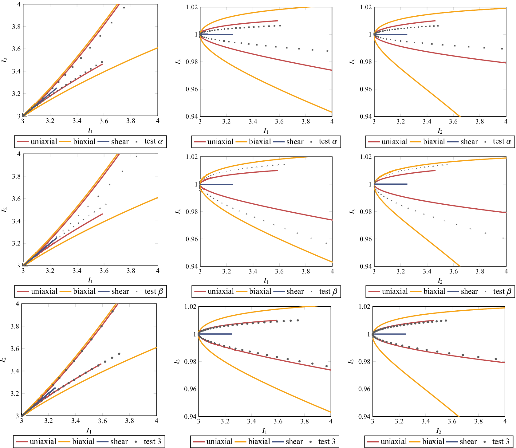
Figure 5. Load paths of the test cases in the invariant space for $ \mu =1.5 $
. First row: test
$ \mu =1.5 $
. First row: test $ \alpha $
, second row: test
$ \alpha $
, second row: test $ \beta $
, and third row: mixed shear-tension test. First column:
$ \beta $
, and third row: mixed shear-tension test. First column: $ {I}_1-{I}_2 $
plane, second column:
$ {I}_1-{I}_2 $
plane, second column: $ {I}_1-{I}_3 $
plane, third column:
$ {I}_1-{I}_3 $
plane, third column: $ {I}_2-{I}_3 $
plane.
$ {I}_2-{I}_3 $
plane.
Furthermore, a mixed shear-tension deformation mode is investigated, compare “test 3” in Fernández et al. (Reference Fernández, Jamshidian, Böhlke, Kersting and Weeger2021). Here, the deformation gradient
 $$ \boldsymbol{F}=\left[\begin{array}{ccc}1+0.5\lambda & 0.4\lambda & 0\\ {}0& {F}_{22}& 0\\ {}0& 0& {F}_{33}\end{array}\right],\hskip1em {P}_{22}={P}_{33}=0,\hskip1em \lambda \in \left[-1,1\right] $$
is considered, where $ {F}_{22},{F}_{33} $
are calculated by solving the corresponding system of equations. Surprisingly, despite seeming like a more general deformation gradient than equation (32), in the invariant space, this load case is almost identical to uniaxial tension (cf. Figure 5, third column). Thus, the mixed shear-tension test as introduced in Fernández et al. (Reference Fernández, Jamshidian, Böhlke, Kersting and Weeger2021) for a metamaterial model with cubic symmetry, is not as general for isotropic materials, and for most investigations to follow, test
$ {F}_{22},{F}_{33} $
are calculated by solving the corresponding system of equations. Surprisingly, despite seeming like a more general deformation gradient than equation (32), in the invariant space, this load case is almost identical to uniaxial tension (cf. Figure 5, third column). Thus, the mixed shear-tension test as introduced in Fernández et al. (Reference Fernández, Jamshidian, Böhlke, Kersting and Weeger2021) for a metamaterial model with cubic symmetry, is not as general for isotropic materials, and for most investigations to follow, test $ \alpha $
and
$ \alpha $
and $ \beta $
are applied.
$ \beta $
are applied.
It should be noted that in this work, only isotropic material behavior is considered, which allows for the generation of general deformation modes using only main diagonal components of the deformation gradient. For general anisotropic materials, compare Ebbing (Reference Ebbing2010), this strategy might not be applicable. Then, other data generation strategies such as extracting deformation modes out of complex FE simulations (Kalina et al., Reference Kalina, Linden, Brummund and Kästner2023), or sampling the space of physically sensible deformation gradients (Kunc and Fritzen, Reference Kunc and Fritzen2019) could be applied. Nevertheless, the test cases applied in this work and particularly Figure 5 demonstrates that the generality of a deformation mode should always be investigated in the invariant space, rather than only investigating deformation gradients, compare Kalina et al. (Reference Kalina, Linden, Brummund, Metsch and Kästner2022) and Kalina et al. (Reference Kalina, Linden, Brummund and Kästner2023).
5.1.2. Model preparation and calibration
In this example, the pICNN architectures with an arbitrary functional relationship in the parameter $ t $
are applied, that is, Type 1–3. The hyperparameters, that is, the number of nodes and layers, of the different pICNN architectures described in Section 4.2 are chosen such that they are in the same order of magnitude for all models. The number of nodes and layers are visualized in Figure 3. The total number of trainable parameters for the models using the Type 1–3 pICNNs are 272, 516, and 580, respectively. For the model calibration, the loss function given as the mean squared error
$ t $
are applied, that is, Type 1–3. The hyperparameters, that is, the number of nodes and layers, of the different pICNN architectures described in Section 4.2 are chosen such that they are in the same order of magnitude for all models. The number of nodes and layers are visualized in Figure 3. The total number of trainable parameters for the models using the Type 1–3 pICNNs are 272, 516, and 580, respectively. For the model calibration, the loss function given as the mean squared error
 $$ \mathrm{MSE}=\frac{1}{9 lmn}\sum \limits_{i=1}^l\sum \limits_{j=1}^m\frac{1}{w_{ij}}\sum \limits_{k=1}^n{\left\Vert {}^{ij k}\boldsymbol{P}-\boldsymbol{P}\left({}^{ik}\boldsymbol{F};{\hskip0.35em }^jt\right)\right\Vert}^2 $$
is minimized. Here, the outer loop over $ i $
corresponds to the
$ i $
corresponds to the $ l $
load paths in the calibration dataset. Each load path is combined with
$ l $
load paths in the calibration dataset. Each load path is combined with $ m $
different, fixed
$ m $
different, fixed $ t $
values, where the sum over
$ t $
values, where the sum over $ j $
corresponds to the values of
$ j $
corresponds to the values of $ t $
. Finally, for one fixed combination of load path and parameter
$ t $
. Finally, for one fixed combination of load path and parameter $ t $
, the weight is calculated according to the norm
$ t $
, the weight is calculated according to the norm
 $$ {w}_{ij}=\frac{1}{n}\sum \limits_{k=1}^n\left\Vert {}^{ij k}\boldsymbol{P}\right\Vert, $$
and the innermost sum over $ k $
corresponds to the
$ k $
corresponds to the $ n $
different deformation gradients. For the evaluation of the loss after the model calibration, all weights are set to one, that is,
$ n $
different deformation gradients. For the evaluation of the loss after the model calibration, all weights are set to one, that is, $ {w}_{ij}=1 $
. The models are implemented in TensorFlow 2.10.0, using Python 3.10.9. For the optimization, the Adam optimizer is used with a learning rate of 0.002 and
$ {w}_{ij}=1 $
. The models are implemented in TensorFlow 2.10.0, using Python 3.10.9. For the optimization, the Adam optimizer is used with a learning rate of 0.002 and $ \mathrm{7,000} $
epochs. The full batch of training data is used with TensorFlow’s default batch size. Although the number of parameters is in the same order of magnitude for all model architectures, it should be noted that the calibration process is affected by many hyperparameters (Nakkiran et al., Reference Nakkiran, Kaplun, Bansal, Yang, Barak and Sutskever2021), which suggests that the optimal calibration process for each pICNN architecture might be different. Nevertheless, with the applied calibration strategy, all model architectures show excellent results in the examples to follow.
$ \mathrm{7,000} $
epochs. The full batch of training data is used with TensorFlow’s default batch size. Although the number of parameters is in the same order of magnitude for all model architectures, it should be noted that the calibration process is affected by many hyperparameters (Nakkiran et al., Reference Nakkiran, Kaplun, Bansal, Yang, Barak and Sutskever2021), which suggests that the optimal calibration process for each pICNN architecture might be different. Nevertheless, with the applied calibration strategy, all model architectures show excellent results in the examples to follow.
Study I: For the calibration dataset, the uniaxial, biaxial, and shear loads are combined with $ t\in \left\{0,0.2,0.4,0.6,0.8,1\right\} $
. Thus, the calibration dataset consists of
$ t\in \left\{0,0.2,0.4,0.6,0.8,1\right\} $
. Thus, the calibration dataset consists of $ \mathrm{1,818} $
tuples. For the test dataset, the test load cases (test
$ \mathrm{1,818} $
tuples. For the test dataset, the test load cases (test $ \alpha $
and test
$ \alpha $
and test $ \beta $
) are combined with all remaining 195 values for
$ \beta $
) are combined with all remaining 195 values for $ t $
not included in the calibration, thus consisting of
$ t $
not included in the calibration, thus consisting of $ \mathrm{19,695} $
tuples. For this study, the PANN model as described in Section 4 is applied, with three different versions using the pICNN architectures Type 1–3 as described in 4.2. Each model is calibrated five times to each parametrization case, where the model with the worst test loss is excluded.
$ \mathrm{19,695} $
tuples. For this study, the PANN model as described in Section 4 is applied, with three different versions using the pICNN architectures Type 1–3 as described in 4.2. Each model is calibrated five times to each parametrization case, where the model with the worst test loss is excluded.
Study II: For the calibration dataset, the uniaxial, biaxial, and shear-tension loads are combined with $ t\in \left\{0,0.1,0.9,1\right\} $
, yielding a calibration dataset with
$ t\in \left\{0,0.1,0.9,1\right\} $
, yielding a calibration dataset with $ \mathrm{1,212} $
tuples. For the test dataset, the mixed shear-tension test is combined with the 197 remaining values for
$ \mathrm{1,212} $
tuples. For the test dataset, the mixed shear-tension test is combined with the 197 remaining values for $ t $
not included in the calibration, thus consisting of
$ t $
not included in the calibration, thus consisting of $ \mathrm{19,897} $
tuples. For this study, the model as described in Section 4 is adapted in such a way that it does not include the normalization term equation (13). Here, the pICNN architecture Type 1 is applied. One model instance with the normalization condition, and one without is calibrated. The models are calibrated one time to the parametrization case A.
$ \mathrm{19,897} $
tuples. For this study, the model as described in Section 4 is adapted in such a way that it does not include the normalization term equation (13). Here, the pICNN architecture Type 1 is applied. One model instance with the normalization condition, and one without is calibrated. The models are calibrated one time to the parametrization case A.
5.1.3. Results
Study I: In Table 1, the MSE values of the calibrated models are presented for all pICNN architectures and all parametrization cases. In general, all pICNN architectures are able to interpolate the data for all parametrization cases and also show excellent performance on the test dataset for all parametrizations. In general, the pICNN Type 3 performs better on the test dataset than the remaining architectures. However, due to the simplicity of the examined data, no premature conclusions about the general performance of the different architectures should be drawn. Even the architecture with the lowest complexity might be sufficiently flexible in practical applications. Furthermore, the reduced complexity of Type 1 might be advantageous in some applications, for example, when implementing the model in a finite-element code. The MSEs were evaluated for the test load cases (test $ \alpha $
and
$ \alpha $
and $ \beta $
) and all values of
$ \beta $
) and all values of $ t $
are visualized in Figure 6. Not surprisingly, the models perform better for values of
$ t $
are visualized in Figure 6. Not surprisingly, the models perform better for values of $ t $
which were included in the model calibration. In particular for parametrization A and C, the pICNN Type 3 performs way better than the other architectures. This superior performance of pICNN Type 3 might be explained by the multiplicative operations between invariants and parameters in its architecture, which enables it to more accurately and easily describe the Neo-Hookean potential used for data generation, compare equation (19). Note that, when leaving the training values of
$ t $
which were included in the model calibration. In particular for parametrization A and C, the pICNN Type 3 performs way better than the other architectures. This superior performance of pICNN Type 3 might be explained by the multiplicative operations between invariants and parameters in its architecture, which enables it to more accurately and easily describe the Neo-Hookean potential used for data generation, compare equation (19). Note that, when leaving the training values of $ t $
, the MSE increases quite quickly for Type 1 and 2, which could be a sign of overfitting in the parameter
$ t $
, the MSE increases quite quickly for Type 1 and 2, which could be a sign of overfitting in the parameter $ t $
. For parametrization B, the pICNN architecture 3 shows a similar behavior compared to the other pICNN architectures. While pICNN Type 1 and 2 have quite similar prediction qualities between different calibration instances, pICNN Type 3 has a higher discrepancy between different calibration instances, as indicated by the shaded areas.
$ t $
. For parametrization B, the pICNN architecture 3 shows a similar behavior compared to the other pICNN architectures. While pICNN Type 1 and 2 have quite similar prediction qualities between different calibration instances, pICNN Type 3 has a higher discrepancy between different calibration instances, as indicated by the shaded areas.
Table 1.
Average $ {\log}_{10} $
MSE for the scalar-valued parametrization
$ {\log}_{10} $
MSE for the scalar-valued parametrization

Note. Four best-calibrated model instances for study I for all parametrization cases and pICNN types.

Figure 6. Evaluation of the test cases. Continuous lines denote the average of $ {\log}_{10} $
MSE, while shaded areas denote the standard deviation of
$ {\log}_{10} $
MSE, while shaded areas denote the standard deviation of $ {\log}_{10} $
MSE.
$ {\log}_{10} $
MSE.
For the following investigation, a random instance of the four trained models was chosen. In Figure 7, some stress predictions of the models are visualized for the parametrization case C. On the top row, a model using a Type 1 pICNN is evaluated on test $ \alpha $
, while on the bottom row, a model using a Type 3 pICNN is evaluated on test
$ \alpha $
, while on the bottom row, a model using a Type 3 pICNN is evaluated on test $ \beta $
. On the left-hand side, the models are evaluated for values of
$ \beta $
. On the left-hand side, the models are evaluated for values of $ t $
used in the calibration, while on the right-hand side, the models are evaluated for values of
$ t $
used in the calibration, while on the right-hand side, the models are evaluated for values of $ t $
not used in the calibration. In all cases, the model has to extrapolate in the load case. The interpolation is excellent for both evaluated models. For Type 1, the evaluation for
$ t $
not used in the calibration. In all cases, the model has to extrapolate in the load case. The interpolation is excellent for both evaluated models. For Type 1, the evaluation for $ t=0.3 $
shows some visible deviations from the ground truth. This case has a
$ t=0.3 $
shows some visible deviations from the ground truth. This case has a $ {\log}_{10} $
MSE of −2.66. Thus, with the MSEs of Figure 6 in mind, this is a representative case for the less good model predictions. And still, the prediction quality might be good enough for most practical applications. The pICNN Type 3 is able to also perfectly make predictions at
$ {\log}_{10} $
MSE of −2.66. Thus, with the MSEs of Figure 6 in mind, this is a representative case for the less good model predictions. And still, the prediction quality might be good enough for most practical applications. The pICNN Type 3 is able to also perfectly make predictions at $ t=0.5 $
, although the magnitude of the stress components differs by a factor of
$ t=0.5 $
, although the magnitude of the stress components differs by a factor of $ \approx $
4 for different values of
$ \approx $
4 for different values of $ t $
.
$ t $
.

Figure 7. Results for parametrization case C, evaluated for the test cases. Dashed lines and points denote the data, while continuous lines denote the model prediction.
Study II: In Figure 8, a comparison is made between a model which fulfills the normalization condition of equation (13) by construction and one which only learns to approximate the condition through the calibration dataset. This case includes values of $ t $
only on the edges of its parameter domain and is here evaluated for the value in the middle. While for the model which fulfills the normalization condition by construction, there are some significant deviations from the ground truth, it still fulfills the normalization condition in an exact way. The model which does not fulfill the normalization condition by construction has to learn it by the data which fulfill this property. While this indeed works out for the values of
$ t $
only on the edges of its parameter domain and is here evaluated for the value in the middle. While for the model which fulfills the normalization condition by construction, there are some significant deviations from the ground truth, it still fulfills the normalization condition in an exact way. The model which does not fulfill the normalization condition by construction has to learn it by the data which fulfill this property. While this indeed works out for the values of $ t $
included in the calibration dataset, for the case visualized here it is violated quite obviously. This is despite the used deformation mode, the mixed shear-tension test, being very close to the uniaxial deformation mode contained in the training set, compare Figure 5. This example demonstrates the benefit of fulfilling mechanical conditions by construction, in particular for the generalization of the model.
$ t $
included in the calibration dataset, for the case visualized here it is violated quite obviously. This is despite the used deformation mode, the mixed shear-tension test, being very close to the uniaxial deformation mode contained in the training set, compare Figure 5. This example demonstrates the benefit of fulfilling mechanical conditions by construction, in particular for the generalization of the model.

Figure 8. Results for parametrization case C, evaluated for the mixed shear-tension case. In this case, the model was only calibrated on the edges of the parameter domain of $ t $
, and evaluated in the middle. Dashed lines and points denote the data, while continuous lines denote the model prediction.
$ t $
, and evaluated in the middle. Dashed lines and points denote the data, while continuous lines denote the model prediction.
5.2. Vector-valued parametrization with monotonicity condition
5.2.1. Data generation
In the next example, the Neo-Hookean potential
 $$ {\psi}^{\mathrm{nh}}\left({I}_1,{I}_3;\boldsymbol{t}\right)=\frac{\mu \left(\boldsymbol{t}\right)}{2}\left({I}_1-3-2\ln \sqrt{I_3}\right)+\frac{\lambda }{2}{\left(\sqrt{I_3}-1\right)}^2\hskip0.35em $$
is considered, where $ \mu \left(\boldsymbol{t}\right) $
is parametrized in
$ \mu \left(\boldsymbol{t}\right) $
is parametrized in $ \boldsymbol{t}=\left({G}^0,{\tau}^0\right)\in {\left[0,1\right]}^2 $
and
$ \boldsymbol{t}=\left({G}^0,{\tau}^0\right)\in {\left[0,1\right]}^2 $
and $ \lambda =100=\mathrm{const} $
. The parametrization
$ \lambda =100=\mathrm{const} $
. The parametrization
 $$ {\displaystyle \begin{array}{llll}& \mu \left(\boldsymbol{t}\right)=2.5\hskip0.35em \tanh \hskip0.35em {H}^v,\hskip2em & & {H}^v=1.7\hskip0.35em {G}^2\hskip0.35em \ln \hskip0.35em \hat{\tau},\\ {}& \hat{G}=0.6+0.4{G}^0,\hskip2em & & \hat{\tau}=1.5+4.5{\tau}^0,\end{array}} $$
is inspired by a 3D printing process, where a liquid photopolymer resin is hardened by exposing it to ultraviolet light for a given time, compare Valizadeh et al. (Reference Valizadeh, Al Aboud, Dörsam and Weeger2021). The properties of the final solid material depend on both the light intensity, which is determined through the greyscale value $ \hat{G} $
, and the time
$ \hat{G} $
, and the time $ \hat{\tau} $
the light is applied on the resin. Here, these two parameters are parameterized in a physically sensible range through
$ \hat{\tau} $
the light is applied on the resin. Here, these two parameters are parameterized in a physically sensible range through $ {G}^0 $
, which is associated with the light intensity, and
$ {G}^0 $
, which is associated with the light intensity, and $ {\tau}^0 $
, which is associated with the exposure time for which the light is applied on the resin. The parametrization consists of three ideas. First of all, the shear modulus
$ {\tau}^0 $
, which is associated with the exposure time for which the light is applied on the resin. The parametrization consists of three ideas. First of all, the shear modulus $ \mu $
is influenced by both
$ \mu $
is influenced by both $ {G}^0 $
and
$ {G}^0 $
and $ {\tau}^0 $
. In particular, the same shear modulus can be achieved by different combinations of
$ {\tau}^0 $
. In particular, the same shear modulus can be achieved by different combinations of $ \left({G}^0,{\tau}^0\right) $
. This is reflected by the intermediate quantity
$ \left({G}^0,{\tau}^0\right) $
. This is reflected by the intermediate quantity $ {H}^v $
, compare equation (37). Secondly, the shear modulus is bounded from above, which is reflected by the
$ {H}^v $
, compare equation (37). Secondly, the shear modulus is bounded from above, which is reflected by the $ \tanh $
function which receives
$ \tanh $
function which receives $ {H}^v $
as an input. Lastly, the shear modulus is a monotonically increasing function in
$ {H}^v $
as an input. Lastly, the shear modulus is a monotonically increasing function in $ \left({G}^0,{\tau}^0\right) $
, which reflects the physical observation that the shear modulus increases when increasing the light intensity or the light exposure time. In Figure 9, these characteristics are visualized.
$ \left({G}^0,{\tau}^0\right) $
, which reflects the physical observation that the shear modulus increases when increasing the light intensity or the light exposure time. In Figure 9, these characteristics are visualized.

Figure 9. Dependency of the shear modulus $ \mu $
on the vector-valued, 3D printing-inspired parametrization in terms of
$ \mu $
on the vector-valued, 3D printing-inspired parametrization in terms of $ \left({G}^0,,,\hskip0.35em ,{\tau}^0\right) $
.
$ \left({G}^0,,,\hskip0.35em ,{\tau}^0\right) $
.
The deformation gradients are sampled as described in Section 5.1.1. For the calibration dataset, nine parameter combinations $ \boldsymbol{t}=\left({G}^0,{\tau}^0\right) $
are sampled, compare Figure 9. For the test dataset, two
$ \boldsymbol{t}=\left({G}^0,{\tau}^0\right) $
are sampled, compare Figure 9. For the test dataset, two $ \mu $
-iso-curves are considered for
$ \mu $
-iso-curves are considered for $ \mu \in \left\{1.4,2.4\right\} $
, compare Figure 9. For each iso-curve, 100
$ \mu \in \left\{1.4,2.4\right\} $
, compare Figure 9. For each iso-curve, 100 $ \left({G}^0,{\tau}^0\right) $
tuples are sampled. Overall, this results in a calibration dataset with
$ \left({G}^0,{\tau}^0\right) $
tuples are sampled. Overall, this results in a calibration dataset with $ \mathrm{2,727} $
tuples and a test dataset with
$ \mathrm{2,727} $
tuples and a test dataset with $ \mathrm{20,200} $
tuples.
$ \mathrm{20,200} $
tuples.
5.2.2. Model preparation and calibration
In this example, the pICNN architecture with a monotonically increasing functional relationship in the parameter $ \boldsymbol{t} $
is applied, that is, Type 1 M. The number of nodes and layers is visualized in Figure 3, where the total number of trainable parameters is 280. For the model calibration, all stress values are normalized by the inverse mean Frobenius norm of all tuples in the calibration dataset. Then, the loss function is given as the mean squared error
$ \boldsymbol{t} $
is applied, that is, Type 1 M. The number of nodes and layers is visualized in Figure 3, where the total number of trainable parameters is 280. For the model calibration, all stress values are normalized by the inverse mean Frobenius norm of all tuples in the calibration dataset. Then, the loss function is given as the mean squared error
 $$ \mathrm{MSE}=\frac{1}{9n}\sum \limits_{i=1}^n\frac{1}{w_i}{\left\Vert {}^i\boldsymbol{P}-\boldsymbol{P}\left({}^i\boldsymbol{F};{\hskip0.35em }^i\boldsymbol{t}\right)\right\Vert}^2 $$
is minimized, where $ n $
is the number of tuples in the calibration dataset. The sample weight
$ n $
is the number of tuples in the calibration dataset. The sample weight
 $$ {w}_i=\left\Vert {}^i\boldsymbol{P}\right\Vert +1\ge 1 $$
is calculated for each single tuple and used to encourage better accuracy of the model when predicting small stress values. For the optimization, the SLSQP optimizer is used.
5.2.3. Results
In Table 2, the average $ {\log}_{10} $
MSE of the four model instances with the best test MSE, as well as the
$ {\log}_{10} $
MSE of the four model instances with the best test MSE, as well as the $ {\log}_{10} $
MSE of the model instance with the best test MSE are presented. The performance on both the calibration and the test dataset is excellent. In Figure 10, the stress predictions for the test cases for
$ {\log}_{10} $
MSE of the model instance with the best test MSE are presented. The performance on both the calibration and the test dataset is excellent. In Figure 10, the stress predictions for the test cases for $ {H}^v\in \left\{1.4,2.4\right\} $
are visualized for the best model instance. The calibrated model is evaluated for 100 different
$ {H}^v\in \left\{1.4,2.4\right\} $
are visualized for the best model instance. The calibrated model is evaluated for 100 different $ \left({G}^0,{\tau}^0\right) $
combinations on each
$ \left({G}^0,{\tau}^0\right) $
combinations on each $ \mu $
-iso-curve. For
$ \mu $
-iso-curve. For $ {H}^v=2.4 $
, the model perfectly learns the invariance of
$ {H}^v=2.4 $
, the model perfectly learns the invariance of $ {H}^v $
in
$ {H}^v $
in $ \left({G}^0,{\tau}^0\right) $
. Thus, the model predictions for different
$ \left({G}^0,{\tau}^0\right) $
. Thus, the model predictions for different $ \left({G}^0,{\tau}^0\right) $
combinations are practically identical. For
$ \left({G}^0,{\tau}^0\right) $
combinations are practically identical. For $ {H}^v=1.4 $
, the model predictions slightly differ for different
$ {H}^v=1.4 $
, the model predictions slightly differ for different $ \left({G}^0,{\tau}^0\right) $
combinations, which is indicated by the (fairly small) shaded areas in Figure 10. This can be traced back to the larger sensitivity of the ground truth models material parameter
$ \left({G}^0,{\tau}^0\right) $
combinations, which is indicated by the (fairly small) shaded areas in Figure 10. This can be traced back to the larger sensitivity of the ground truth models material parameter $ \mu $
at smaller
$ \mu $
at smaller $ {H}^V $
values, compare equation (36) and Figure 9. Overall, the model performs excellent, in particular with regard to the low amount of
$ {H}^V $
values, compare equation (36) and Figure 9. Overall, the model performs excellent, in particular with regard to the low amount of $ \left({G}^0,,,\hskip0.35em ,{\tau}^0\right) $
samples in the calibration dataset.
$ \left({G}^0,,,\hskip0.35em ,{\tau}^0\right) $
samples in the calibration dataset.
Table 2. Average $ {\log}_{10} $
MSE for the vector-valued parametrization
$ {\log}_{10} $
MSE for the vector-valued parametrization
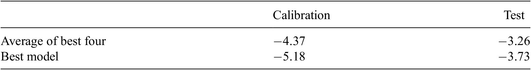
Note. Four best-calibrated model instances.

Figure 10. Model prediction for the test cases. Dashed lines and points denote the data, while lines and shaded areas depict the calibrated model evaluated for different parameter combinations $ \left({G}^0,{\tau}^0\right) $
on
$ \left({G}^0,{\tau}^0\right) $
on $ {H}^v $
iso-curves.
$ {H}^v $
iso-curves.
6. Conclusion
In the present work, a NN-based constitutive model for parametrized hyperelasticity is proposed. The model is formulated in such a way that it fulfills all common constitutive conditions of hyperelasticity by construction, without being too restrictive in the parametric dependencies of the model. In particular, by applying pICNNs, the model fulfills the polyconvexity condition, while still being able to represent arbitrary functional relationships in the additional parameter. In addition, a polyconvex potential is proposed which is monotonic in the additional parameters.
As a first proof of concept, the model is calibrated to data generated with an analytical potential which depends on one scalar-valued parameter. Different pICNN architectures with different complexities are examined, where all architectures performed excellent. However, due to the simplicity of the examined data, no premature conclusions about the general performance of the different architectures should be drawn. Even the architecture with the lowest complexity might be sufficiently flexible in practical applications, while its easier and thus computationally more efficient model structure can be advantageous. Furthermore, the proposed model is calibrated to data generated with an analytical potential which depends on multiple parameters. In this case, the dependency of the ground truth potential in the parameters is monotonic, and the NN-based potential which by construction is monotonic in the additional parameters is applied. Again, the model shows excellent performance.
The extension of the proposed framework to multiphysical constitutive models, such as electro-elasticity (Klein et al., Reference Klein, Ortigosa, Martínez-Frutos and Weeger2022b), will be straightforward, as well as the application in finite-element analysis (Franke et al., Reference Franke, Klein, Weeger and Betsch2023) and optimization of microstructured materials (Ortigosa et al., Reference Ortigosa, Martínez-Frutos and Gil2023). Furthermore, the application to real-world experimental data of composites or polymer materials with varying constituents is targeted.
Data availability statement
The authors provide access to the simulation data required to reproduce the results through the public GitHub repository at https://github.com/CPShub/sim-data.
Author contribution
Conceptualization: D.K.K., F.J.R., I.V., O.W.; Formal analysis: D.K.K., F.J.R.; Funding acquisition: O.W.; Investigation: F.J.R.; Methodology: D.K.K., F.J.R., I.V., O.W.; Resources: O.W.; Software: D.K.K., F.J.R.; Validation: F.J.R.; Visualization: D.K.K., F.J.R.; Writing—original draft: D.K.K.; Writing—review and editing: D.K.K., F.J.R., I.V., O.W.
Funding statement
This research was supported by the Deutsche Forschungsgemeinschaft (DFG—German Research Foundation)—Grant No. 492770117 and the Graduate School of Computational Engineering within the Centre of Computational Engineering at TU Darmstadt.
Competing interest
The authors declare none.
Ethical standard
The research meets all ethical guidelines, including adherence to the legal requirements of the study country.


 Open access
Comments
No Comments have been published for this article.