


Impact Statement
The development of urban aerial mobility has gained significant momentum in recent years, with notable initiatives such as Airbus’ plan to introduce aerial taxis for the Paris 2024 Olympic Games and Amazon’s exploration of drone delivery services. Within this emerging field, one critical challenge lies in mitigating disturbances experienced by aerial vehicles. The onboard systems must detect aerological perturbations and minimize their impact on the aerodynamic loads (e.g., lift, drag). We propose a new comprehensive framework harnessing data-driven techniques for detecting perturbations and optimizing control actions to effectively mitigate atmospheric disturbances. This research has far-reaching implications for urban air mobility, as it contributes to ensure safe and reliable operations in the presence of disturbed urban aerological conditions.
1. Introduction
Urban air mobility (UAM) is promised to have a flourishing future in the coming years (Johnson et al., Reference Johnson, Silva, Solis, Silva and Solis2018; Straubinger et al., Reference Straubinger, Rothfeld, Shamiyeh, Büchter, Kaiser and Plötner2020). Johnson et al. (Reference Johnson, Silva, Solis, Silva and Solis2018) draw the guidelines for future NASA research for UAM development. Among other challenges, such as electric/hybrid propulsion efficiency, safety, and structural integrity, the issue of disturbance rejection by the onboard flight control system is central to UAM development. Current research describes any type of aerodynamic disturbance of an air vehicle as a gust. Jones et al. (Reference Jones, Cetiner and Smith2022) proposed to categorize gusts into three types: (i) streamwise gusts, (ii) transverse gusts, and (iii) vortex gusts. Streamwise gusts are perturbations parallel to the inflow, transverse gusts are perturbations perpendicular to the inflow, and vortex gusts are bi-directional perturbations stemming from a vortex singularity of circulation ![]() .
.
The gust mitigation literature focuses mainly on transverse gusts, yet it is worth noting that these three types of gusts present specific issues that require dedicated mitigation methods.
Firstly, streamwise gusts induce a time-dependant change in effective Reynolds number, which is not critical at high Reynolds numbers but may induce a strongly non-linear lift response to the perturbation at low to moderate Reynolds numbers. This can be viewed as a quasi-steady effect. Moreover, this effect may be modulated by the presence of a streamwise pressure gradient (supported by the temporal perturbation) that affects flow separation, laminar-to-turbulent transition, and reattachment of the separated shear layer, if any, at low and moderate Reynolds numbers. Furthermore, added mass effects and unsteady effects resulting from feedback effects of the developing wake on the airfoil also come into play, typically by introducing attenuation and phase lag to the quasi-steady lift response. The latter are however general to all types of gusts.
Secondly, in addition to added mass and wake effects, as well as potential changes in effective Reynolds numbers, transverse gusts induce a modification of the effective Angle of Attack (AoA) of the vehicle. For example, a transverse gust with an upwash ![]() impinging an airfoil flying at a zero incidence and velocity
impinging an airfoil flying at a zero incidence and velocity ![]() yields an effective AoA perturbation
yields an effective AoA perturbation ![]() at first order (Von Karman and Sears, Reference Von Karman and Sears1938). The main strategy proposed in the literature consists of actively pitching the airfoil to reject the gust-induced disturbance (Andreu-Angulo and Babinsky, Reference Andreu-Angulo and Babinsky2020, Reference Andreu-Angulo and Babinsky2021, Reference Andreu-Angulo and Babinsky2022; Sedky et al., Reference Sedky, Jones and Lagor2020a, Reference Sedky, Lagor and Jones2020b, Reference Sedky, Gementzopoulos, Andreu-Angulo, Lagor and Jones2022). For instance, Andreu-Angulo and Babinsky (Reference Andreu-Angulo and Babinsky2021) determine the adequate AoA temporal sequence
at first order (Von Karman and Sears, Reference Von Karman and Sears1938). The main strategy proposed in the literature consists of actively pitching the airfoil to reject the gust-induced disturbance (Andreu-Angulo and Babinsky, Reference Andreu-Angulo and Babinsky2020, Reference Andreu-Angulo and Babinsky2021, Reference Andreu-Angulo and Babinsky2022; Sedky et al., Reference Sedky, Jones and Lagor2020a, Reference Sedky, Lagor and Jones2020b, Reference Sedky, Gementzopoulos, Andreu-Angulo, Lagor and Jones2022). For instance, Andreu-Angulo and Babinsky (Reference Andreu-Angulo and Babinsky2021) determine the adequate AoA temporal sequence ![]() to mitigate a transverse gust according to low-order models, by minimizing the lift coefficient at each time step, independently of the consequences of choosing
to mitigate a transverse gust according to low-order models, by minimizing the lift coefficient at each time step, independently of the consequences of choosing ![]() on future lift coefficients. Alternatively, Poudel et al. (Reference Poudel, Yu and Hrynuk2021) investigate an open-loop control strategy using oscillating airfoils to mitigate long-lived transverse gusts.
on future lift coefficients. Alternatively, Poudel et al. (Reference Poudel, Yu and Hrynuk2021) investigate an open-loop control strategy using oscillating airfoils to mitigate long-lived transverse gusts.
Thirdly, vortex gusts introduce new challenges that could previously be ignored for the mitigation of the two other gust types, which we discuss below:
-
• Transverse gusts are described by a predefined spatial distribution of upwash disturbances, which are convected at a fixed velocity towards the airfoil, that is, the airfoil pitch motion does not affect the incoming flow perturbation. This made the minimization of the current lift coefficient at every time step by Andreu-Angulo and Babinsky (Reference Andreu-Angulo and Babinsky2021) a reasonable approximation of an optimal control sequence. Conversely, the sequence of AoAs of an airfoil moving through a gust of vortices affects the vortices’ future positions, which, in turn, requires accounting for the future system’s evolution when choosing
 , making the vortex gust control more delicate (Jones et al., Reference Jones, Cetiner and Smith2022).
 -
• The main effect of transverse gusts on the lift is due to the modification of the AoA, so that only the upwash perturbation at the leading edge is required to establish the proper control law. This information can be obtained by a simple velocity measurement on the airfoil, yet accurate estimations of AoA in turbulent flows are still an open challenge in practice (Gavrilovic et al., Reference Gavrilovic, Bronz, Moschetta and Benard2018). In contrast, vortices have long-distance effects via their induced velocity on the geometry (Biot–Savart law). This suggests that the position and circulation of the vortices—which are parameters that cannot be directly measured with only onboard sensors (da Silva and Colonius, Reference da Silva and Colonius2018; Le Provost and Eldredge, Reference Le Provost and Eldredge2021)—should be known to compute an optimal control.
While experimental control of a wing in disturbed flow by DRL has been investigated by Renn and Gharib (Reference Renn and Gharib2022), methods to mitigate vortex gusts are still scarce in the literature. On the one hand, Herrmann et al. (Reference Herrmann, Brunton, Pohl and Semaan2022) propose a feedforward and feedback strategy controlling the flap of the trailing edge to mitigate the vortex-induced disturbances. On the other hand, Kazarin et al. (Reference Kazarin, Golubev, MacKunis and Moreno2021) aim to solve the robust control problem, which consists of controlling the roll and yaw behavior of an aircraft subjected to unknown and bounded vortex disturbances. However, none of them address the question of the vortex estimation from the onboard measurements. Specifically, Herrmann et al. (Reference Herrmann, Brunton, Pohl and Semaan2022) estimate experimentally the vortices by a velocity sensor upstream of the airfoil, while Kazarin et al. (Reference Kazarin, Golubev, MacKunis and Moreno2021) consider the vortex gust as an unknown disturbance. To address simultaneously the two difficulties encountered when mitigating vortex gusts, the main objective of our work is to develop a new closed-loop non-linear controller. It is built as an artificial neural network (ANN) that actively pitches a flat plate to mitigate the unsteady lift induced by a vortex gust. To do so, the flow behavior is modeled according to the unsteady vortex lattice method (UVLM). The present work proposes to learn this ANN controller using a deep reinforcement learning (DRL) (Sutton and Barto, Reference Sutton and Barto2018) method. DRL is meant to compute optimal controllers for fully observable systems, that is, it requires observing the positions and circulations of the gust vortices at each control time step. To circumvent this issue, a Kalman particle filter (KPF) is proposed on top of the DRL controller to estimate the full state from only onboard measurements.
This paper is organized as follows: Section 2 covers related works which put our contribution in perspective. Section 3 introduces the gust mitigation problem, as well as the UVLM model. Section 4 describes the optimal control problem underlying the mitigation of a vortex gust, as well as the DRL and the KPF algorithms used for its resolution. Finally, in Section 5, we evaluate the performance of the DRL-trained controller, taking the vortices estimated by the KPF as input.
2. Related work
2.1. Deep reinforcement learning for optimal control
In the present work, we model the unsteady lift response to the gust-induced disturbance using the unsteady vortex lattice method (UVLM) (Katz and Plotkin, Reference Katz and Plotkin2001). The controller is based on an artificial neural network (ANN) (Goodfellow et al., Reference Goodfellow, Bengio and Courville2016), which is trained to mitigate the vortex gust through DRL (Sutton and Barto, Reference Sutton and Barto2018). In a DRL approach, the ANN controller is optimized to mitigate the vortex gust through interactions with the UVLM model. The interaction follows a discrete time evolution. At each interaction step, the controller observes the environment’s state ![]() . Then, it computes an action
. Then, it computes an action ![]() , which is applied to the flat plate, triggering a transition in the UVLM model from a state
, which is applied to the flat plate, triggering a transition in the UVLM model from a state ![]() to
to ![]() . Finally, the controller receives a reward
. Finally, the controller receives a reward ![]() depending on the new state of the environment
depending on the new state of the environment ![]() . Based on a collection of samples
. Based on a collection of samples ![]() , the DRL algorithm optimizes the controller parameters such that the state-control sequence
, the DRL algorithm optimizes the controller parameters such that the state-control sequence ![]() minimizes the criterion
minimizes the criterion ![]() , where
, where ![]() is the final time of the simulation. This optimization procedure allows us
is the final time of the simulation. This optimization procedure allows us
-
• to assess the performance loss due to vortex unobservability. Although DRL theory clearly states that
must be a Markov state, that is, contain vortex circulations and vortex positions, we are nevertheless able to train the controller with inputs limited to on-board measurements (non-Markov state) but with no guarantee on the control law optimality. -
• to evaluate multiple levels of control law complexity. DRL allows us to model the control function as either a simple linear combination of its input or as a complex nonlinear function, modeled as an ANN.
The potential application of ANNs for unsteady fluid dynamics has been established since late 1990 (Faller and Schreck, Reference Faller and Schreck1997). In the last few years, ANNs have solved many fluid-related tasks (Brenner et al., Reference Brenner, Eldredge and Freund2019; Brunton et al., Reference Brunton, Noack and Koumoutsakos2020; Garnier et al., Reference Garnier, Viquerat, Rabault, Larcher, Kuhnle and Hachem2021; Brunton and Kutz, Reference Brunton and Kutz2022). For instance, DRL has been used for a large variety of fluid control tasks, such as reducing the drag coefficient of the flow around a cylinder (Rabault et al., Reference Rabault, Kuchta, Jensen, Réglade and Cerardi2019), or diminishing the effort of swimmers leveraging the wake generated by the swimmer ahead (Novati et al., Reference Novati, Verma, Alexeev, Rossinelli, Van Rees and Koumoutsakos2017). Regarding aerodynamics and flight control, DRL has been used to solve a variety of aerodynamic control problems. For instance, Waldock et al. (Reference Waldock, Greatwood, Salama and Richardson2018) showed that DRL agents are able to manage a landing autonomously, and Bøhn et al. (Reference Bøhn, Coates, Moe and Johansen2019) showed that DRL algorithms have a better ability than standard linear controllers to control the pitch, roll, and yaw of an unmanned aerial vehicle. For the specific question of gust mitigation, DRL offers three advantages over the control method described above. First, DRL is designed to optimize a sequence of actions, which is precisely one of the main difficulties when mitigating a vortex gust compared with transverse perturbations. Second, DRL is able to learn a controller directly from the UVLM model, whereas traditional approaches use low-order models to derive the controller (e.g., Andreu-Angulo and Babinsky, Reference Andreu-Angulo and Babinsky2021). Third, ANNs allow for an efficient approximation of strongly nonlinear control laws as well as linear control functions.
2.2. Partial observation and state estimation
In the perspective of a real-world deployment, the DRL-trained controller must have full access to the environment state ![]() , yet some quantities of
, yet some quantities of ![]() , namely the circulations and locations of the gust vortices in the present problem, are not directly measurable with the onboard sensors. This is known as the problem of partial observability, which may lead to performance loss of the controllers (Gunnarson et al., Reference Gunnarson, Mandralis, Novati, Koumoutsakos and Dabiri2021, Paris et al., Reference Paris, Beneddine and Dandois2021). The DRL community proposes adding a recurrent ANN (Rumelhart et al., Reference Rumelhart, Hinton and Williams1986; Elman, Reference Elman1990; Sherstinsky, Reference Sherstinsky2020) on top of the ANN controller architecture to recover the performance loss due to partial knowledge of the environment state. Hausknecht and Stone (Reference Hausknecht and Stone2015), Meng et al. (Reference Meng, Gorbet and Kulić2021), and Yang and Nguyen (Reference Yang and Nguyen2021) show that this method does indeed recover the performance obtained, compared to when the ANN controller has full access to the environment state. In the specific context of vortex estimation, several strategies are investigated in the literature to determine vortex parameters from the onboard measurements (da Silva and Colonius, Reference da Silva and Colonius2018; Darakananda et al., Reference Darakananda, Castro da Silva, Colonius and Eldredge2018; Hou et al., Reference Hou, Darakananda and Eldredge2019; Fukami et al., Reference Fukami, Fukagata and Taira2020; Le Provost and Eldredge, Reference Le Provost and Eldredge2021), but these works focus mostly on configurations with downstream wake vortices, rather than incoming gust vortices. A first approach is to learn the correspondence between the unknown vortices and the measurement using end-to-end machine learning techniques (Hou et al., Reference Hou, Darakananda and Eldredge2019; Fukami et al., Reference Fukami, Fukagata and Taira2020). A second considers the vortex parameters as the internal variables
, namely the circulations and locations of the gust vortices in the present problem, are not directly measurable with the onboard sensors. This is known as the problem of partial observability, which may lead to performance loss of the controllers (Gunnarson et al., Reference Gunnarson, Mandralis, Novati, Koumoutsakos and Dabiri2021, Paris et al., Reference Paris, Beneddine and Dandois2021). The DRL community proposes adding a recurrent ANN (Rumelhart et al., Reference Rumelhart, Hinton and Williams1986; Elman, Reference Elman1990; Sherstinsky, Reference Sherstinsky2020) on top of the ANN controller architecture to recover the performance loss due to partial knowledge of the environment state. Hausknecht and Stone (Reference Hausknecht and Stone2015), Meng et al. (Reference Meng, Gorbet and Kulić2021), and Yang and Nguyen (Reference Yang and Nguyen2021) show that this method does indeed recover the performance obtained, compared to when the ANN controller has full access to the environment state. In the specific context of vortex estimation, several strategies are investigated in the literature to determine vortex parameters from the onboard measurements (da Silva and Colonius, Reference da Silva and Colonius2018; Darakananda et al., Reference Darakananda, Castro da Silva, Colonius and Eldredge2018; Hou et al., Reference Hou, Darakananda and Eldredge2019; Fukami et al., Reference Fukami, Fukagata and Taira2020; Le Provost and Eldredge, Reference Le Provost and Eldredge2021), but these works focus mostly on configurations with downstream wake vortices, rather than incoming gust vortices. A first approach is to learn the correspondence between the unknown vortices and the measurement using end-to-end machine learning techniques (Hou et al., Reference Hou, Darakananda and Eldredge2019; Fukami et al., Reference Fukami, Fukagata and Taira2020). A second considers the vortex parameters as the internal variables ![]() of a known transition model
of a known transition model ![]() , and attempts to estimate them from the sensor measurements
, and attempts to estimate them from the sensor measurements ![]() using Kalman filters (KFs) (da Silva and Colonius, Reference da Silva and Colonius2018, Darakananda et al., Reference Darakananda, Castro da Silva, Colonius and Eldredge2018; Le Provost and Eldredge, Reference Le Provost and Eldredge2021). Here
using Kalman filters (KFs) (da Silva and Colonius, Reference da Silva and Colonius2018, Darakananda et al., Reference Darakananda, Castro da Silva, Colonius and Eldredge2018; Le Provost and Eldredge, Reference Le Provost and Eldredge2021). Here ![]() is the UVLM model, and
is the UVLM model, and ![]() is the operator computing the pressure on the flat plate. This filtering problem consists in finding an estimation sequence
is the operator computing the pressure on the flat plate. This filtering problem consists in finding an estimation sequence ![]() of
of ![]() so that the associated measurement sequence
so that the associated measurement sequence ![]() fits the actual sequence of measurements
fits the actual sequence of measurements ![]() . In the UVLM framework,
. In the UVLM framework, ![]() and h are both non-linearly dependant on
and h are both non-linearly dependant on ![]() , so the classical KF derived by Kalman and Bucy (Reference Kalman and Bucy1961) is not well suited for the present application. To overcome this issue, Julier and Uhlmann (Reference Julier and Uhlmann2004) propose the unscented KF that is able to handle the complete non-linear model. Nevertheless, the computational cost of this approach becomes quickly untractable when the state dimension increases (da Silva and Colonius, Reference da Silva and Colonius2018; Le Provost and Eldredge, Reference Le Provost and Eldredge2021). The alternative to make the computation tractable lies in discretizing the internal state space with a set of particles. KPF (Ristic et al., Reference Ristic, Arulampalam and Gordon2003; Elfring et al., Reference Elfring, Torta and van de Molengraft2021) pairs each particle with its so-called likelihood probability, i.e., the probability that the particle corresponds to the actual state
, so the classical KF derived by Kalman and Bucy (Reference Kalman and Bucy1961) is not well suited for the present application. To overcome this issue, Julier and Uhlmann (Reference Julier and Uhlmann2004) propose the unscented KF that is able to handle the complete non-linear model. Nevertheless, the computational cost of this approach becomes quickly untractable when the state dimension increases (da Silva and Colonius, Reference da Silva and Colonius2018; Le Provost and Eldredge, Reference Le Provost and Eldredge2021). The alternative to make the computation tractable lies in discretizing the internal state space with a set of particles. KPF (Ristic et al., Reference Ristic, Arulampalam and Gordon2003; Elfring et al., Reference Elfring, Torta and van de Molengraft2021) pairs each particle with its so-called likelihood probability, i.e., the probability that the particle corresponds to the actual state ![]() . In the present study, a particle represent a possible description of the gust, i.e. it is a set
. In the present study, a particle represent a possible description of the gust, i.e. it is a set ![]() , where
, where ![]() and
and ![]() are espectively a possible circulation and location for the i-th vortex. At each time step, the KPF computes
are espectively a possible circulation and location for the i-th vortex. At each time step, the KPF computes ![]() as the average of the particles. Concurrently, Evensen (Reference Evensen1994) assumes that the probability distribution of
as the average of the particles. Concurrently, Evensen (Reference Evensen1994) assumes that the probability distribution of ![]() remains Gaussian at any time, and introduces the ensemble KF (EnKF). Because the Gaussian probability distribution is defined by its two first moments, the EnKF only computes the particles’ mean and covariance to compute
remains Gaussian at any time, and introduces the ensemble KF (EnKF). Because the Gaussian probability distribution is defined by its two first moments, the EnKF only computes the particles’ mean and covariance to compute ![]() . The works aiming at estimating wake vortices conducted by Le Provost and Eldredge (Reference Le Provost and Eldredge2021), da Silva and Colonius (Reference da Silva and Colonius2018) and Darakananda et al. (Reference Darakananda, Castro da Silva, Colonius and Eldredge2018) use EnKF because the number of vortices to estimate is consequent (only the EnKF remains tractable in such a situation). In our work, we prefer to use a KPF to estimate the gust vortices because it is known to achieve better estimation accuracy (Pham, Reference Pham2001; Weerts and El Serafy, Reference Weerts and El Serafy2006; Le Provost and Eldredge, Reference Le Provost and Eldredge2021) than EnKF if the number of particles is high enough. It implies that the number of gust vortices to estimate in our configuration remains small compared to that studied by Le Provost and Eldredge (Reference Le Provost and Eldredge2021).
. The works aiming at estimating wake vortices conducted by Le Provost and Eldredge (Reference Le Provost and Eldredge2021), da Silva and Colonius (Reference da Silva and Colonius2018) and Darakananda et al. (Reference Darakananda, Castro da Silva, Colonius and Eldredge2018) use EnKF because the number of vortices to estimate is consequent (only the EnKF remains tractable in such a situation). In our work, we prefer to use a KPF to estimate the gust vortices because it is known to achieve better estimation accuracy (Pham, Reference Pham2001; Weerts and El Serafy, Reference Weerts and El Serafy2006; Le Provost and Eldredge, Reference Le Provost and Eldredge2021) than EnKF if the number of particles is high enough. It implies that the number of gust vortices to estimate in our configuration remains small compared to that studied by Le Provost and Eldredge (Reference Le Provost and Eldredge2021).
3. Problem statement
3.1. The gust mitigation problem
We consider a two-dimensional aerodynamic profile, modeled as a flat plate, flying through a vortex gust consisting of ![]() vortices. The flat plate quarter chord is at coordinates
vortices. The flat plate quarter chord is at coordinates ![]() around which rotation can be performed (see Figure 1). Let
around which rotation can be performed (see Figure 1). Let ![]() ,
, ![]() and
and ![]() be respectively the chord, the incidence and the pitch rate of the flat plate,
be respectively the chord, the incidence and the pitch rate of the flat plate, ![]() the uniform flow velocity parallel to the
the uniform flow velocity parallel to the ![]() direction and
direction and ![]() the fluid density. The gust vortices are modeled according to the so-called Kaufmann model (Kaufmann, Reference Kaufmann1962; Bhagwat and Leishman, Reference Bhagwat and Leishman2002). It aims at adding a viscous core
the fluid density. The gust vortices are modeled according to the so-called Kaufmann model (Kaufmann, Reference Kaufmann1962; Bhagwat and Leishman, Reference Bhagwat and Leishman2002). It aims at adding a viscous core ![]() in a potential vortex, with
in a potential vortex, with ![]() set to
set to ![]() here. The Kaufmann vortices then behave as potential vortices away from the core, while the fluid inside the viscous core undergoes a solid-like rotation. In this work, the gust consists of
here. The Kaufmann vortices then behave as potential vortices away from the core, while the fluid inside the viscous core undergoes a solid-like rotation. In this work, the gust consists of ![]() trains of
trains of ![]() Kaufmann vortices, with each train being spaced by
Kaufmann vortices, with each train being spaced by ![]() and each vortex having the same circulation
and each vortex having the same circulation ![]() . We denote the position of the j-th vortex of the i-th train as
. We denote the position of the j-th vortex of the i-th train as ![]() . Such a vortex induces a velocity perturbation at the point
. Such a vortex induces a velocity perturbation at the point ![]() modeled as
modeled as ![]() where
where ![]() is the unit vector normal to
is the unit vector normal to ![]() oriented clockwise, and
oriented clockwise, and ![]() is given as
is given as


Figure 1. Geometry of the problem.
We define the so-called radius of influence ![]() of a vortex as the maximum distance such that the vortex-induced velocity is, arbitrarily, greater than
of a vortex as the maximum distance such that the vortex-induced velocity is, arbitrarily, greater than ![]() . In the following, we denote the discrete convective time
. In the following, we denote the discrete convective time ![]() , the normalized gust vortex circulation
, the normalized gust vortex circulation ![]() , the normalized spacing between the vortices
, the normalized spacing between the vortices ![]() , the flat plate’s lift
, the flat plate’s lift ![]() , the lift coefficient
, the lift coefficient ![]() , the normalized lift coefficient
, the normalized lift coefficient ![]() , the normalized incidence
, the normalized incidence ![]() and its temporal derivative
and its temporal derivative ![]() .
.
In this work, we consider six types of vortex gusts, classified in three categories:
-
• The one-vortex gust, the two-vortices gust, the three-vortices gust, and the five-vortices gust (Figure 2a–d). We refer to these gusts as 1, 2, 3, and 5, respectively. These gusts are composed of vortices of circulation
. For each of the gusts, the i-th vortex is initialized to the coordinate where and is randomly chosen uniformly in . -
• The 2×3-vortices gust (Figure 2e). This gust is composed of two trains of three vortices of circulation
that are initialized at coordinates where and is randomly chosen uniformly in . We refer to this gust as 2×3 in the following. -
• The 3×2-vortices gust (Figure 2f). This gust is composed of three trains of two vortices of circulation
that are initialized at coordinates where and is randomly chosen unifomly in . We refer to this gust as 3×2 in the following.
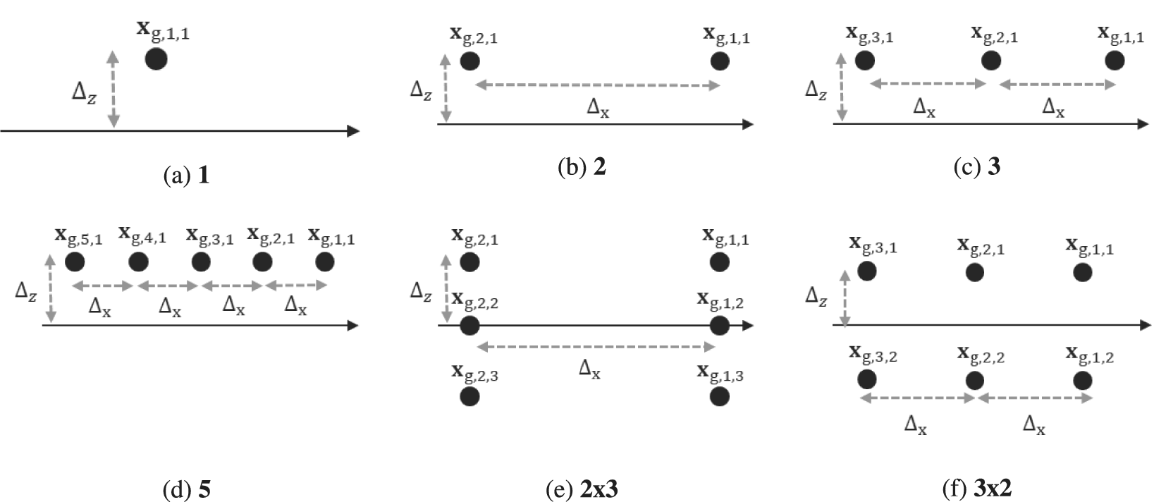
Figure 2. Sketch of the vortex gusts. Panels (a–d) represent the one-vortex gust, the two-vortices gust, the three-vortices gust and the five-vortices gust, respectively. Panel (e) represents the 2×3-vortices gust, and (f) represents the 3×2-vortices gust.
The objective of this paper is to mitigate the lift perturbations induced by each of these gusts parameterized by ![]() and
and ![]() . These parameters are chosen uniformly in
. These parameters are chosen uniformly in ![]() and
and ![]() respectively.
respectively. ![]() is evaluated with the maximum value of
is evaluated with the maximum value of ![]() , i.e.
, i.e. ![]() , which corresponds to
, which corresponds to ![]() (Eq. 1). The control is performed by pitching the flat plate around its quarter chord, at a control frequency
(Eq. 1). The control is performed by pitching the flat plate around its quarter chord, at a control frequency ![]() , so that the criterion
, so that the criterion ![]() described as follows is minimal:
described as follows is minimal:

where ![]() is the final convective simulation time, and the desired lift coefficient is here chosen as
is the final convective simulation time, and the desired lift coefficient is here chosen as ![]() for the sake of simplicity.
for the sake of simplicity.
3.2. Environment modeling
The temporal evolution of the gust-induced lift is computed using the UVLM (Katz and Plotkin, Reference Katz and Plotkin2001). It is a medium-fidelity tool, valid under the assumption of an incompressible potential flow, which in particular, involves an infinite Reynolds number. The method approximates the overall flow as the sum of the incident flow ![]() and the induced velocities due to a discrete set of vortex singularities. Among these vortices,
and the induced velocities due to a discrete set of vortex singularities. Among these vortices, ![]() are the gust vortices,
are the gust vortices, ![]() are located along the flat plate’s chord (bound vortices), and
are located along the flat plate’s chord (bound vortices), and ![]() are shed from the Trailing Edge (TE). In the following, we refer to the set of flat plate, wake and gust vortices as
are shed from the Trailing Edge (TE). In the following, we refer to the set of flat plate, wake and gust vortices as ![]() ,
, ![]() and
and ![]() respectively. We respectively denote by
respectively. We respectively denote by ![]() ,
, ![]() the circulation and the position of the i-th profile vortex, and by
the circulation and the position of the i-th profile vortex, and by ![]() ,
, ![]() the circulation and the position of the j-th wake vortex. The flow induced by a single gust vortex is modeled as in Eq. 1, whereas the flow induced by the i-th vortex of the profile (resp. of the wake)
the circulation and the position of the j-th wake vortex. The flow induced by a single gust vortex is modeled as in Eq. 1, whereas the flow induced by the i-th vortex of the profile (resp. of the wake) ![]() (resp.
(resp. ![]() ) is obtained using the Biot-Savart law:
) is obtained using the Biot-Savart law:

At each time step, we seek the circulation of the profile vortices so that the non-penetration condition is satisfied:

with ![]() and n is the normal to the flat plate.
and n is the normal to the flat plate. ![]() is the velocity induced by the pitch motion about the quarter chord:
is the velocity induced by the pitch motion about the quarter chord: ![]() where
where ![]() is the coordinate of the quarter chord.
is the coordinate of the quarter chord.
The circulation of the profile vortices ![]() is computed by recasting Eq. 4 into a linear system:
is computed by recasting Eq. 4 into a linear system:

with ![]() the so-called influence matrix, whose size is
the so-called influence matrix, whose size is ![]() , and the components
, and the components ![]() represent the velocity induced by the j-th profile vortex on the i-th profile vortex projected along
represent the velocity induced by the j-th profile vortex on the i-th profile vortex projected along ![]() . Once
. Once ![]() is computed, the conservation of the circulation (Kelvin condition) is enforced by shedding a new wake element from the trailing edge. Its circulation
is computed, the conservation of the circulation (Kelvin condition) is enforced by shedding a new wake element from the trailing edge. Its circulation ![]() is given according to the Kelvin equation:
is given according to the Kelvin equation:
Note that the wake (and gust) circulations remain constant during the simulation because the viscous dissipation of the vortices is neglected.
The transition between time ![]() and time
and time ![]() is performed by advecting the wake vortices and the gust vortices by the total flow velocity
is performed by advecting the wake vortices and the gust vortices by the total flow velocity ![]() using a first-order difference scheme:
using a first-order difference scheme:
Finally, the lift is computed according to Katz and Plotkin (Reference Katz and Plotkin2001) as:

where ![]() ,
, ![]() being the circulation density, and the integration of
being the circulation density, and the integration of ![]() is performed according to the Simpson’s method.
is performed according to the Simpson’s method.
In the present work, the number of profile vortices is ![]() and the convection time increment is set to
and the convection time increment is set to ![]() . In Appendix A, we assess our UVLM solver on several test cases consisting of (i) an impulsive pitch motion, (ii) a sinusoidal pitch motion, and (iii) an interaction of the (uncontrolled) airfoil with a vortex disturbance.
. In Appendix A, we assess our UVLM solver on several test cases consisting of (i) an impulsive pitch motion, (ii) a sinusoidal pitch motion, and (iii) an interaction of the (uncontrolled) airfoil with a vortex disturbance.
4. Methods
We aim to solve the optimal control problem by finding the control law for the flat plate’s pitch rate ![]() that minimizes the optimality criterion
that minimizes the optimality criterion ![]() defined in Eq. 2, when the profile flies through the vortex gusts described in Section 3. In addition, the inputs of the control law are limited to an observation vector
defined in Eq. 2, when the profile flies through the vortex gusts described in Section 3. In addition, the inputs of the control law are limited to an observation vector ![]() composed of onboard measurements:
composed of onboard measurements:
where ![]() refers to the circulation at the Leading Edge (LE) at time
refers to the circulation at the Leading Edge (LE) at time ![]() . According to Katz and Plotkin (Reference Katz and Plotkin2001),
. According to Katz and Plotkin (Reference Katz and Plotkin2001), ![]() is related to a pressure measurement as
is related to a pressure measurement as ![]() , where
, where ![]() is the pressure difference between the upper and lower surface at the flat plate’s LE. We consider that at time
is the pressure difference between the upper and lower surface at the flat plate’s LE. We consider that at time ![]() , the profile has no wake, no circulation, no initial pitch rate and that the angle of attack is set at
, the profile has no wake, no circulation, no initial pitch rate and that the angle of attack is set at ![]() .
.
4.1. Resolution of the gust mitigation problem
We model this optimal control problem as a finite horizon deterministic Markov decision problem (MDP) (Puterman, Reference Puterman2014). At each discrete time ![]() , the controller takes a new
, the controller takes a new ![]() based on the state of the environment
based on the state of the environment ![]() , that triggers the transition of the environment state from
, that triggers the transition of the environment state from ![]() to
to ![]() according to the UVLM model described in Section 3.2. To ensure the problem is a MDP, the Markovian property should be satisfied. It implies that determining
according to the UVLM model described in Section 3.2. To ensure the problem is a MDP, the Markovian property should be satisfied. It implies that determining ![]() requires only the knowledge of
requires only the knowledge of ![]() and
and ![]() , regardless of previous values of
, regardless of previous values of ![]() and
and ![]() . Thus, according to the UVLM model equations (Eqs. 5–8),
. Thus, according to the UVLM model equations (Eqs. 5–8), ![]() must contain:
must contain:
Note that the airfoil vortices ![]() are not part of the environment state, since they are computed from
are not part of the environment state, since they are computed from ![]() according to Eq. 5. After each transition, the controller observes a user-defined reward of this transition:
according to Eq. 5. After each transition, the controller observes a user-defined reward of this transition: ![]() . The resolution of this finite-horizon MDP consists of finding the decision function
. The resolution of this finite-horizon MDP consists of finding the decision function ![]() such that the induced trajectory
such that the induced trajectory ![]() minimizes
minimizes ![]() .
.
The MDP described above is solved using DRL (Sutton and Barto, Reference Sutton and Barto2018) where the control function, i.e the flat plate controller, is an artificial neural network (ANN) (Goodfellow et al., Reference Goodfellow, Bengio and Courville2016). The input of the ANN controller is the state of the environment ![]() and it outputs a pitch rate
and it outputs a pitch rate ![]() . The DRL algorithm chosen here is the twin delayed deep deterministic policy gradient algorithm (TD3) (Fujimoto et al., Reference Fujimoto, Hoof and Meger2018). In parallel to the ANN controller, TD3 learns the value function
. The DRL algorithm chosen here is the twin delayed deep deterministic policy gradient algorithm (TD3) (Fujimoto et al., Reference Fujimoto, Hoof and Meger2018). In parallel to the ANN controller, TD3 learns the value function ![]() also as an ANN. Here, these ANNs are fully-connected networks, composed of zero, one, or two hidden layers of
also as an ANN. Here, these ANNs are fully-connected networks, composed of zero, one, or two hidden layers of ![]() neurons each. To optimize its behavior, the ANN controller undergoes a variety of simulated gusts, that is, the gust parameters
neurons each. To optimize its behavior, the ANN controller undergoes a variety of simulated gusts, that is, the gust parameters ![]() and
and ![]() are randomly and uniformly initialized in
are randomly and uniformly initialized in ![]() and
and ![]() . At each convective time increment
. At each convective time increment ![]() , the ANN controller takes a new
, the ANN controller takes a new ![]() , triggering a transition in the MDP. The result of this transition is gathered by the algorithm as a sample
, triggering a transition in the MDP. The result of this transition is gathered by the algorithm as a sample ![]() . Then, based on a random batch from the samples collected so far, the parameters of both ANNs are optimized using the stochastic gradient descent algorithm on the TD3 loss functions. The ANN controller being deterministic, a Gaussian exploration noise of mean zero and constant standard deviation
. Then, based on a random batch from the samples collected so far, the parameters of both ANNs are optimized using the stochastic gradient descent algorithm on the TD3 loss functions. The ANN controller being deterministic, a Gaussian exploration noise of mean zero and constant standard deviation ![]() is added to the ANN controller output. In this case, a training run lasts approximately between 8 hours, for the one-vortex gust and 24 hours, for the five-vortex gust, on two CPUs.
is added to the ANN controller output. In this case, a training run lasts approximately between 8 hours, for the one-vortex gust and 24 hours, for the five-vortex gust, on two CPUs.
4.2. Estimation of non-observable quantities
The ANN controller trained using TD3 must take as input the environment state vector ![]() (Eq. 11), but some variables of
(Eq. 11), but some variables of ![]() , namely
, namely ![]() ,
, ![]() are not part of the available onboard measurements (Eq. 10). To render the problem more realistic, and because the impact of the wake on the dynamics of the environment can be assumed to be negligible compared to that of the gust,
are not part of the available onboard measurements (Eq. 10). To render the problem more realistic, and because the impact of the wake on the dynamics of the environment can be assumed to be negligible compared to that of the gust, ![]() is not estimated in the present work. We estimate
is not estimated in the present work. We estimate ![]() from
from ![]() (Eq. 10) using a KPF (Ristic et al., Reference Ristic, Arulampalam and Gordon2003; Elfring et al., Reference Elfring, Torta and van de Molengraft2021). We denote by
(Eq. 10) using a KPF (Ristic et al., Reference Ristic, Arulampalam and Gordon2003; Elfring et al., Reference Elfring, Torta and van de Molengraft2021). We denote by ![]() the estimate of the circulation and position of the gust vortices. We also denote
the estimate of the circulation and position of the gust vortices. We also denote ![]() the environment state estimated by the KPF:
the environment state estimated by the KPF:

This ![]() vector features the state variables measured by the onboard measurements as well as the KPF estimate of the gust vortices. As stated in the introduction, the KPF computes
vector features the state variables measured by the onboard measurements as well as the KPF estimate of the gust vortices. As stated in the introduction, the KPF computes ![]() as the internal variables of a system of first-order differential equations:
as the internal variables of a system of first-order differential equations:  , that corresponds here to the dynamics described by the UVLM (Section 3.2). This system of equations is paired with a measurement operator
 ![]() that computes the circulation
that computes the circulation ![]() at the LE, if
at the LE, if ![]() were the actual vortices:
were the actual vortices:  . According to Eq. 8, the non-viscous flow assumption and the above wake simplification,
 ![]() is given as follows:
is given as follows:

where ![]() is the flow stemming from the j-th estimated gust vortex (Eq. 1), and
is the flow stemming from the j-th estimated gust vortex (Eq. 1), and ![]() is the flow stemming from the estimated flat plate vortices. It is computed according to Eq. 3 with the circulation of the estimated vortices
is the flow stemming from the estimated flat plate vortices. It is computed according to Eq. 3 with the circulation of the estimated vortices ![]() calculated as in Eq. 5 but neglecting the wake:
calculated as in Eq. 5 but neglecting the wake:

In particular, the ![]() operator computes
operator computes ![]() as the component of
as the component of ![]() at the LE.
at the LE.
The KPF computes the gust vortex estimation sequence  such that the associated sequence
 ![]() maximizes its so-called likelihood probability, i.e.
maximizes its so-called likelihood probability, i.e. ![]() where
where ![]() is the Gaussian distribution with mean
is the Gaussian distribution with mean ![]() and standard deviation
and standard deviation ![]() . We briefly present here how the KPF proceeds to compute
. We briefly present here how the KPF proceeds to compute  . The KPF discretizes the gust vortex space of size
 ![]() as a set of
as a set of ![]() particles. At the simulation initialization, the KPF initializes randomly the particles. As the simulation continues, the KPF (i) propagates each particle through
particles. At the simulation initialization, the KPF initializes randomly the particles. As the simulation continues, the KPF (i) propagates each particle through ![]() , (ii) computes the LE circulation associated to each particle, (iii) assimilates a new measure of
, (ii) computes the LE circulation associated to each particle, (iii) assimilates a new measure of ![]() , (iv) calculates the estimate. For the KPF implementation, we used the practical implementation provided by Elfring et al. (Reference Elfring, Torta and van de Molengraft2021). The only difference is that instead of using a constant value of
, (iv) calculates the estimate. For the KPF implementation, we used the practical implementation provided by Elfring et al. (Reference Elfring, Torta and van de Molengraft2021). The only difference is that instead of using a constant value of ![]() , we set
, we set ![]() (see Appendix C).
(see Appendix C).
To summarize, we propose to solve the gust mitigation problem described in Section 3 by training an ANN controller using DRL. During the training, the ANN controller has full access to the gust state ![]() and to the onboard measurement
and to the onboard measurement ![]() (Eq. 10). However, during deployment, the ANN controller does not have access to the actual gust state, instead, the ANN controller takes as input the environment state estimate
(Eq. 10). However, during deployment, the ANN controller does not have access to the actual gust state, instead, the ANN controller takes as input the environment state estimate ![]() (Eq. 12) performed by a KPF. In the following, we refer to this controller as the KPF controller. A scheme of the KPF controller is presented in Figure 3.
(Eq. 12) performed by a KPF. In the following, we refer to this controller as the KPF controller. A scheme of the KPF controller is presented in Figure 3.

Figure 3. Scheme of the KPF controller.
5. Results
In this section, we take advantage of DRL’s versatility on both control law’s shape and inputs to assess the performance gap between (i) linear controllers and non-linear controllers and (ii) full knowledge of the gust vortices and inputs restricted to onboard measurements. Furthermore, we investigate the recoverability of the performance loss due to partial observations using online estimations of the gust vortices performed by a KPF. In this perspective, we present the performance of the linear and non-linear KPF controllers, described in Section 4, on the gust mitigation problems that consist in mitigating the gust configurations 1, 2, 3, 5 described in Figure 2. As a comparison, we also introduce (i) the Full Observation ANN controller (FO controller), that is, an idealized controller taking as inputs the actual values of ![]() instead of the KPF’s gust reconstruction, and (ii) the Partial Observation ANN controller (PO controller) which stems from training TD3 with inputs limited to the on-board measurements
instead of the KPF’s gust reconstruction, and (ii) the Partial Observation ANN controller (PO controller) which stems from training TD3 with inputs limited to the on-board measurements ![]() . Note that the latter does not solve an MDP because
. Note that the latter does not solve an MDP because ![]() and
and ![]() are not sufficient to compute
are not sufficient to compute ![]() . The corresponding system is a partially observable MDP, for which there is no guarantee that there is an optimal control defined only on
. The corresponding system is a partially observable MDP, for which there is no guarantee that there is an optimal control defined only on ![]() . This section is organized as follows: in Section 5.1, we conduct a cross-analysis of the controller performance regarding its shape complexity and inputs, then in Section 5.2 we present the gust reconstruction and the performance recovery performed by the KPF controller, in Section 5.3 we present in detail the control law learned through DRL and their associated lift mitigation. Finally, in Section 5.4 we extend the discussion to gusts composed of more vortices than estimated by the KPF.
. This section is organized as follows: in Section 5.1, we conduct a cross-analysis of the controller performance regarding its shape complexity and inputs, then in Section 5.2 we present the gust reconstruction and the performance recovery performed by the KPF controller, in Section 5.3 we present in detail the control law learned through DRL and their associated lift mitigation. Finally, in Section 5.4 we extend the discussion to gusts composed of more vortices than estimated by the KPF.
5.1. Shape of the optimal control function
The aim of this section is to explore the characteristics of the optimal control function for the present gust mitigation problem. Specifically, we analyze the complexity of the control function necessary for this problem and examine how the control functions depend on the unobservable gust vortex position and circulation. Three controller architectures are evaluated, with respectively zero, one, and two hidden layers, the hidden layer activation function is ReLu, and the output layer activation function is ![]() . Note that the zero hidden layer architecture corresponds to a linear combination of the inputs with the
. Note that the zero hidden layer architecture corresponds to a linear combination of the inputs with the ![]() function applied on top. We designate the FO (resp. PO) controller with
function applied on top. We designate the FO (resp. PO) controller with ![]() hidden layers as the
hidden layers as the ![]() -FO controller (resp.
-FO controller (resp. ![]() -PO controller). The performance of those controllers is evaluated across gust configurations 1, 2, 3, and 5, as illustrated in Figure 2, with initial gust transverse position set to zero for the sake of repeatability. Note that separate controllers have been trained to mitigate each of these vortex gust configurations. To ensure a fair comparison, each controller is trained using the same protocol: the same number of simulations and the same sequence of initial states. Additionally, the same set of hyper-parameters, as detailed in Appendix B, is used for each training run. These hyper-parameters are inspired by the default parameters in the OpenAI Spinning Up DRL library. It is important to note that the stochastic noise used during ANN optimization can lead to variations in ANN controller performance (Berger et al., Reference Berger, Ramo, Guillet, Lahire, Martin, Jardin, Rachelson and Bauerheim2024). To mitigate this effect, we present the performance of 15 controllers trained with different stochastic noises. These controllers are selected based on the lowest
-PO controller). The performance of those controllers is evaluated across gust configurations 1, 2, 3, and 5, as illustrated in Figure 2, with initial gust transverse position set to zero for the sake of repeatability. Note that separate controllers have been trained to mitigate each of these vortex gust configurations. To ensure a fair comparison, each controller is trained using the same protocol: the same number of simulations and the same sequence of initial states. Additionally, the same set of hyper-parameters, as detailed in Appendix B, is used for each training run. These hyper-parameters are inspired by the default parameters in the OpenAI Spinning Up DRL library. It is important to note that the stochastic noise used during ANN optimization can lead to variations in ANN controller performance (Berger et al., Reference Berger, Ramo, Guillet, Lahire, Martin, Jardin, Rachelson and Bauerheim2024). To mitigate this effect, we present the performance of 15 controllers trained with different stochastic noises. These controllers are selected based on the lowest ![]() criterion evaluation during their respective training processes (i.e., the final one is not necessarily chosen). We present in Appendix B, the learning curves for 1 and under
criterion evaluation during their respective training processes (i.e., the final one is not necessarily chosen). We present in Appendix B, the learning curves for 1 and under ![]() ,
, ![]() control.
control.
To compare different types of controllers, we introduce the mitigation efficiency as: ![]() , where
, where ![]() represents the
represents the ![]() criterion obtained under control-free conditions, and
criterion obtained under control-free conditions, and ![]() represents the
represents the ![]() criterion obtained using control method X (i.e.,
criterion obtained using control method X (i.e., ![]() -FO,
-FO, ![]() -PO,
-PO, ![]() -KPF). The closer
-KPF). The closer ![]() is to one, the more effectively control method X mitigates the uncontrolled lift disturbance. Figure 4 shows
is to one, the more effectively control method X mitigates the uncontrolled lift disturbance. Figure 4 shows ![]() for the
for the ![]() -FO,
-FO, ![]() -PO control methods for each of the 15 controllers across various gusts. Each controller is assigned a single
-PO control methods for each of the 15 controllers across various gusts. Each controller is assigned a single ![]() value, which is the averaged performance over
value, which is the averaged performance over ![]() and
and ![]() . It is important to note that the
. It is important to note that the ![]() -FO,
-FO, ![]() -FO controllers exhibit catastrophic behavior
-FO controllers exhibit catastrophic behavior ![]() for case 5 with
for case 5 with ![]() and
and ![]() . Since this behavior is only observed in a very specific scenario and over a small range of
. Since this behavior is only observed in a very specific scenario and over a small range of ![]() and
and ![]() , we do not include these configurations in the results presented here and leave this issue for future investigation.
, we do not include these configurations in the results presented here and leave this issue for future investigation.

Figure 4. Controller performances across the gusts. ![]() ,
, ![]() ,
, ![]() , respectively, represent the efficiency of the
, respectively, represent the efficiency of the ![]() -FO controller, the
-FO controller, the ![]() -FO controller, the
-FO controller, the ![]() -FO controller.
-FO controller. ![]() ,
, ![]() ,
, ![]() , respectively, represent the efficiency of the
, respectively, represent the efficiency of the ![]() -PO controller, the
-PO controller, the ![]() -PO controller, the
-PO controller, the ![]() -PO controller. The efficiency values are displayed for 1 in (a), 2 in (b), 3 in (c), and 5 in (d); each value has been obtained as the averaged
-PO controller. The efficiency values are displayed for 1 in (a), 2 in (b), 3 in (c), and 5 in (d); each value has been obtained as the averaged ![]() for a single controller and over
for a single controller and over ![]() and
and ![]() .
.
Linearity of the optimal command law with respect to ![]() . Figure 4 shows that the best linear and non-linear FO controllers achieve mitigation efficiency higher than
. Figure 4 shows that the best linear and non-linear FO controllers achieve mitigation efficiency higher than ![]() for each of the gust, therefore they are all able to efficiently mitigate the gust-induced lift. For 2, 3, 5 the efficiency gap between the best FO controllers seems marginal, but for 1 the mitigation efficiency gap between the best
for each of the gust, therefore they are all able to efficiently mitigate the gust-induced lift. For 2, 3, 5 the efficiency gap between the best FO controllers seems marginal, but for 1 the mitigation efficiency gap between the best ![]() -FO and
-FO and ![]() -FO controllers is significant, about 10%. Adding complexity to the control function also significantly reduce the variability of performance between training runs. In fact, the variability between
-FO controllers is significant, about 10%. Adding complexity to the control function also significantly reduce the variability of performance between training runs. In fact, the variability between ![]() values (
values (![]() ) is far less significant than for
) is far less significant than for ![]() values (
values (![]() ). However, the
). However, the ![]() controller does not show any clear advantage over the
controller does not show any clear advantage over the ![]() controller (
controller (![]() ) neither regarding the maximum mitigation efficiency nor its variability. From those results, we conclude that the optimal control function is well represented by an ANN with no hidden layers, even if the DRL algorithm is not able to accurately approximate it at each training run.
) neither regarding the maximum mitigation efficiency nor its variability. From those results, we conclude that the optimal control function is well represented by an ANN with no hidden layers, even if the DRL algorithm is not able to accurately approximate it at each training run.
Non-linearity of the optimal command law with respect to ![]() . Figure 4 shows that, unlike the
. Figure 4 shows that, unlike the ![]() -FO controller, the
-FO controller, the ![]() -PO controller is not able to mitigate the lift coefficient induced by 1, 2, and 3. Precisely
-PO controller is not able to mitigate the lift coefficient induced by 1, 2, and 3. Precisely ![]() ranges, with high variability, between
ranges, with high variability, between ![]() and
and ![]() . Interestingly, for
. Interestingly, for ![]() , the
, the ![]() -PO controller still observes strong disparity but also observes a significant improvement of the best controller (
-PO controller still observes strong disparity but also observes a significant improvement of the best controller (![]() , against
, against ![]() for 1, 2, 3), which is a mitigation efficiency comparable to that of the best FO controllers. Unlike the FO controllers, adding non-linearities in the PO controller architecture significantly impacts the maximum efficiency reached by the
for 1, 2, 3), which is a mitigation efficiency comparable to that of the best FO controllers. Unlike the FO controllers, adding non-linearities in the PO controller architecture significantly impacts the maximum efficiency reached by the ![]() -PO controllers. One can see that the
-PO controllers. One can see that the ![]() controller reaches, for 1, 2, 3 maximum mitigation efficiencies significantly higher than the
controller reaches, for 1, 2, 3 maximum mitigation efficiencies significantly higher than the ![]() -PO controller but with a comparable disparity. The efficiency loss between the
-PO controller but with a comparable disparity. The efficiency loss between the ![]() controller and the
controller and the ![]() controller is still remarkable for 1 and 2 but is less clear for 3. Furthermore, adding more non-linearities in the PO controller architecture both significantly increases the maximum efficiency and reduces its variability. In fact, one can see that for 1, 2, 3 the maximum efficiencies of the
controller is still remarkable for 1 and 2 but is less clear for 3. Furthermore, adding more non-linearities in the PO controller architecture both significantly increases the maximum efficiency and reduces its variability. In fact, one can see that for 1, 2, 3 the maximum efficiencies of the ![]() -PO controllers outperform the maximum efficiencies of the
-PO controllers outperform the maximum efficiencies of the ![]() -PO controllers, and the efficiency variability seems to have also been reduced for 2, 3, 5. In addition, one can see that, except for 1, the efficiency of the
-PO controllers, and the efficiency variability seems to have also been reduced for 2, 3, 5. In addition, one can see that, except for 1, the efficiency of the ![]() controllers appears similar to that of the
controllers appears similar to that of the ![]() controllers, both in terms of maximum performance and variability. We therefore conclude from these results that the optimal control function can be (i) well approximated by the
controllers, both in terms of maximum performance and variability. We therefore conclude from these results that the optimal control function can be (i) well approximated by the ![]() controller, or (ii) quite well approximated by a nonlinear combination of
controller, or (ii) quite well approximated by a nonlinear combination of ![]() .
.
5.2. Recoverability of the FO controller performances
Now that the performance of the FO and PO controllers has been outlined, we examine the ability of the KPF controller to reconstruct the vortex gusts and restore the FO controller’s mitigation level.
As explained in Section 4.2, the KPF controller estimates the environment state ![]() to compute
to compute ![]() , while the controller is kept the same as the FO controller (no retraining). Consequently, to retrieve the FO controller’s level of performance, it is imperative that the KPF estimates the gust vortices as accurately as possible. The estimation of the KPF depends on two parameters: the number of particles
, while the controller is kept the same as the FO controller (no retraining). Consequently, to retrieve the FO controller’s level of performance, it is imperative that the KPF estimates the gust vortices as accurately as possible. The estimation of the KPF depends on two parameters: the number of particles ![]() and the measurement noise
and the measurement noise ![]() . One can notice that the set of particles at time
. One can notice that the set of particles at time ![]() is included in the initial set of particles convected by the flow (Section 4.2). Thus, to accurately estimate the gust vortices, it is imperative that particles similar to the actual gust vortices (in terms of location and circulation) are represented in the initial set of particles. Therefore, we aim to initialize, within the limit of
is included in the initial set of particles convected by the flow (Section 4.2). Thus, to accurately estimate the gust vortices, it is imperative that particles similar to the actual gust vortices (in terms of location and circulation) are represented in the initial set of particles. Therefore, we aim to initialize, within the limit of ![]() particles, a hundred particles similar to the gust vortices, that is, with one-chord uncertainty in the vortex positions and 10% uncertainty in the vortex circulation. Appendix C shows the probability of a particle to be initialized as each gust with a one-chord position uncertainty and a 10% circulation uncertainty. These probabilities vary from
particles, a hundred particles similar to the gust vortices, that is, with one-chord uncertainty in the vortex positions and 10% uncertainty in the vortex circulation. Appendix C shows the probability of a particle to be initialized as each gust with a one-chord position uncertainty and a 10% circulation uncertainty. These probabilities vary from ![]() for 1 to
for 1 to ![]() for 3. For 5 this probability varies from
for 3. For 5 this probability varies from ![]() for
for ![]() to
to ![]() for
for ![]() . Consequently, we decide to use
. Consequently, we decide to use ![]() ,
, ![]() ,
, ![]() and
and ![]() particles for 1, 2, 3, and 5, respectively. Note that for 5, even with the entire particle budget allocated, only a few particles (resp. no particle) are initialized near the actual vortices for the case
particles for 1, 2, 3, and 5, respectively. Note that for 5, even with the entire particle budget allocated, only a few particles (resp. no particle) are initialized near the actual vortices for the case ![]() (resp.
(resp. ![]() ). The measurement noise
). The measurement noise ![]() is set accordingly, which means that when the vortices are well represented in the particle set, we use a low measurement noise and a large measurement noise otherwise. Precisely
is set accordingly, which means that when the vortices are well represented in the particle set, we use a low measurement noise and a large measurement noise otherwise. Precisely ![]() for 1, 2, and 3, and
for 1, 2, and 3, and ![]() for 5.
for 5.
5.2.1. KPF controller’s performance recovery
To visualize the KPF controller performance recovery, Figure 5 shows ![]() for each of the three controller architectures depending on the associated
for each of the three controller architectures depending on the associated ![]() , when the controller undergoes 1, 2, 3, and 5 (Figure 5). Each controller is represented by a red dot whose x-component represents
, when the controller undergoes 1, 2, 3, and 5 (Figure 5). Each controller is represented by a red dot whose x-component represents ![]() and the y-component represents
and the y-component represents ![]() , so the closer the red dot is to the line
, so the closer the red dot is to the line ![]() , the better the KPF controller recovers the mitigation level of the associated FO controller. In addition, we display the efficiency of each PO controller as a green dot located along the line
, the better the KPF controller recovers the mitigation level of the associated FO controller. In addition, we display the efficiency of each PO controller as a green dot located along the line ![]() . Thus, controllers verifying
. Thus, controllers verifying ![]() see the red dot to the right of the green dot, and controllers verifying
see the red dot to the right of the green dot, and controllers verifying ![]() see the red dot above the green dot. Note that the axis limits are set to
see the red dot above the green dot. Note that the axis limits are set to ![]() , so controllers with negative
, so controllers with negative ![]() are not displayed.
are not displayed.

Figure 5. KPF controllers’ performance recovery. ![]() ,
, ![]() ,
, ![]() are displayed, for 1, 2, 3, 5 under
are displayed, for 1, 2, 3, 5 under ![]() ,
, ![]() ,
, ![]() controllers.
controllers. ![]() represent
represent ![]() =
=![]() for each of the 15 controllers and
for each of the 15 controllers and ![]() represent
represent ![]() displayed along the line
displayed along the line ![]() (—–). Each of the
(—–). Each of the ![]() value given for 1, 2, 3 (resp. 5) are averaged over
value given for 1, 2, 3 (resp. 5) are averaged over ![]() (
(![]() ) and
) and ![]() . Note that the axis’ limits have been set to
. Note that the axis’ limits have been set to ![]() and therefore controllers with
and therefore controllers with ![]() are not displayed.
are not displayed.
These results show that adding a KPF to a DRL-trained controller is a good methodology for the problem of mitigating vortex gusts from onboard measurements. Figure 5 shows that, for 1, 2, 3, some KPF controllers recover well the efficiency of the associated FO controller. This translates into a significant improvement in the performance of the best ![]() -KPF controllers and the best
-KPF controllers and the best ![]() -KPF controllers compared with the best
-KPF controllers compared with the best ![]() -PO controllers and the best
-PO controllers and the best ![]() -PO controllers. However, no clear advantage of the best
-PO controllers. However, no clear advantage of the best ![]() -KPF controllers is found over the best
-KPF controllers is found over the best ![]() -PO controllers, but this is mostly because the performance gap between the best
-PO controllers, but this is mostly because the performance gap between the best ![]() -FO controller and the best
-FO controller and the best ![]() -PO controller is smaller than for the two other architectures.
-PO controller is smaller than for the two other architectures.
Even if the best KPF controllers perform well at recovering the FO controllers’ mitigation level for 1, 2, 3, we notice a strong variability in the mitigation efficiency of the KPF controllers. For example, the ![]() -KPF controller recovers well the attenuation level of the
-KPF controller recovers well the attenuation level of the ![]() -FO controller for 2 and 3, whereas most
-FO controller for 2 and 3, whereas most ![]() -KPF controllers perform poorly for 1. Furthermore, the variability does not seem to be linked to any specific gust type or control architecture. For example, the same
-KPF controllers perform poorly for 1. Furthermore, the variability does not seem to be linked to any specific gust type or control architecture. For example, the same ![]() -KPF controller has low variability for 2 (Figure 5f), but high variability for 1 (Figure 5c), and 1 can be attenuated either with low variability by the
-KPF controller has low variability for 2 (Figure 5f), but high variability for 1 (Figure 5c), and 1 can be attenuated either with low variability by the ![]() -KPF controller, or with high variability by the
-KPF controller, or with high variability by the ![]() -KPF controller.
-KPF controller.
The gust 5 must be viewed from a different perspective than the other three gusts. The first difference is that ![]() plays an important role. Specifically, for the cases
plays an important role. Specifically, for the cases ![]() (Figure 5j–l), the best KPF controllers maintain a reasonable mitigation efficiency since the best
(Figure 5j–l), the best KPF controllers maintain a reasonable mitigation efficiency since the best ![]() are close to their associated
are close to their associated ![]() . But in the case of
. But in the case of ![]() , the performance recovery is significantly reduced compared to the cases with higher
, the performance recovery is significantly reduced compared to the cases with higher ![]() . Furthermore, their performance is inferior to the best PO controllers. The
. Furthermore, their performance is inferior to the best PO controllers. The ![]() -KPF controllers also see their recovery capability reduced compared to the other gusts.
-KPF controllers also see their recovery capability reduced compared to the other gusts.
5.2.2. Gust reconstruction
To further analyse the results of the KPF controller, we study the reconstruction of both the circulation at the LE and the position and circulation of the gusts. We present here the reconstructions performed by the five ![]() -KPF controllers, which are built on top of the five
-KPF controllers, which are built on top of the five ![]() -FO controllers that achieve the lowest
-FO controllers that achieve the lowest ![]() criterion evaluation. (For 1, we present the reconstruction averaged over only four controllers because the fifth is not representative.) We restrict our results to the best controllers because, as explained in the next section, the accuracy of the estimation can vary depending on the controller chosen. We refer to the position of the i-th gust vortex as
criterion evaluation. (For 1, we present the reconstruction averaged over only four controllers because the fifth is not representative.) We restrict our results to the best controllers because, as explained in the next section, the accuracy of the estimation can vary depending on the controller chosen. We refer to the position of the i-th gust vortex as ![]() and to its KPF estimate as
and to its KPF estimate as ![]() .
.
We display in Figure 6 ![]() for each of the gusts with
for each of the gusts with ![]() and
and ![]() , where
, where ![]() (resp.
(resp. ![]() ) is the circulation at the LE induced by the actual gust vortices (resp. the estimated gust vortices) under KPF control. Note that the denominator is clipped under
) is the circulation at the LE induced by the actual gust vortices (resp. the estimated gust vortices) under KPF control. Note that the denominator is clipped under ![]() , because the measurement used for the particles update is itself clipped under
, because the measurement used for the particles update is itself clipped under ![]() (see Section 4.2). For 1, the relative error between
(see Section 4.2). For 1, the relative error between ![]() and
and ![]() has three remarkable stages (Figure 6-a): (i) for
has three remarkable stages (Figure 6-a): (i) for ![]() the error is around 20%, (ii) for
the error is around 20%, (ii) for ![]() the error is characterized by sharp variations of high amplitudes, and (iii) for
the error is characterized by sharp variations of high amplitudes, and (iii) for ![]() the error is of low amplitude, that is, lower than 5%. The decrease in estimation error throughout the simulation is due to the KPF methodology (Section 4.2). Indeed, when initializing the simulation, the KPF computes
the error is of low amplitude, that is, lower than 5%. The decrease in estimation error throughout the simulation is due to the KPF methodology (Section 4.2). Indeed, when initializing the simulation, the KPF computes ![]() as the LE circulation induced by a gust vortex estimated as the mean of a random distribution (since no data is available.) As the simulation continues, the KPF acquires new observations of
as the LE circulation induced by a gust vortex estimated as the mean of a random distribution (since no data is available.) As the simulation continues, the KPF acquires new observations of ![]() and refines the estimate of the vortex so that the sequence of
and refines the estimate of the vortex so that the sequence of ![]() corresponds to the sequence of
corresponds to the sequence of ![]() . However, we notice high amplitude errors when the gust vortex is close to the profile (
. However, we notice high amplitude errors when the gust vortex is close to the profile (![]() in Figure 6a). We can advance two reasons to explain this error: (i) when the vortices are close to the profile, the velocity perturbation induced by the vortices varies sharply with the position of the vortices, and is therefore more sensitive to estimation errors (Eq. 1), (ii) wake vortices are no more negligible in
in Figure 6a). We can advance two reasons to explain this error: (i) when the vortices are close to the profile, the velocity perturbation induced by the vortices varies sharply with the position of the vortices, and is therefore more sensitive to estimation errors (Eq. 1), (ii) wake vortices are no more negligible in ![]() , while they were neglected in the derivation of
, while they were neglected in the derivation of ![]() . The trend observed for 1 is still valid for the other three gusts. However, a singular case is worth to be mentioned. For 5, the MSE between
. The trend observed for 1 is still valid for the other three gusts. However, a singular case is worth to be mentioned. For 5, the MSE between ![]() and
and ![]() is two orders of magnitude higher than for 1, 2, and 3. This result correlates with the discussion of the particle budget above: for 5, the number of particles is not high enough, which reduces the accuracy of the estimate of
is two orders of magnitude higher than for 1, 2, and 3. This result correlates with the discussion of the particle budget above: for 5, the number of particles is not high enough, which reduces the accuracy of the estimate of ![]() in this case.
in this case.

Figure 6. Error ![]() for 1 (a), 2 (b), 3 (c), and 5 (d). The dashed lines represent the cases
for 1 (a), 2 (b), 3 (c), and 5 (d). The dashed lines represent the cases ![]() .
. ![]() has been evaluated for
has been evaluated for ![]() . Solid lines represent the average quantities, and the colored areas are the associated standard deviations. The gray areas report the presence of a gust vortex near the profile.
. Solid lines represent the average quantities, and the colored areas are the associated standard deviations. The gray areas report the presence of a gust vortex near the profile.
As a complementary result, we also present in Figures 7 and 8 the gust reconstruction performed by the KPF controller. Those reconstructions have been made for ![]() and
and ![]() . The estimation of the gust circulation
. The estimation of the gust circulation ![]() and the estimation of the longitudinal position of the gust vortices
and the estimation of the longitudinal position of the gust vortices ![]() are shown. Here, the transverse distance of the vortices from the profile is negligible compared to the longitudinal distance, so we approximate the positions of the vortices to their longitudinal positions and present the estimate of the transverse positions in Appendix D. First, the KPF needs time to accurately estimate the gusts. According to Figures 7 and 8, it estimates accurately 1, 2 and 3 after
are shown. Here, the transverse distance of the vortices from the profile is negligible compared to the longitudinal distance, so we approximate the positions of the vortices to their longitudinal positions and present the estimate of the transverse positions in Appendix D. First, the KPF needs time to accurately estimate the gusts. According to Figures 7 and 8, it estimates accurately 1, 2 and 3 after ![]() ,
, ![]() and
and ![]() units of convective time respectively. Note that the KPF accurately estimates the gust vortices when they pass by the LE. The reason for this estimation delay is that, at the initialization of the simulation, the estimated gust vortex is considered to be the mean of a random distribution (Section 4.2), and then the KPF assimilates observations of
units of convective time respectively. Note that the KPF accurately estimates the gust vortices when they pass by the LE. The reason for this estimation delay is that, at the initialization of the simulation, the estimated gust vortex is considered to be the mean of a random distribution (Section 4.2), and then the KPF assimilates observations of ![]() to refine its reconstruction. Thus, prior to the convection times mentioned above, the KPF estimates the gust vortices far upstream of their actual positions and with an overestimated circulation. Then, the KPF estimates the vortices with an error on
to refine its reconstruction. Thus, prior to the convection times mentioned above, the KPF estimates the gust vortices far upstream of their actual positions and with an overestimated circulation. Then, the KPF estimates the vortices with an error on ![]() of less than 10% and an error on
of less than 10% and an error on ![]() of less than
of less than ![]() . Note that this accuracy holds for each pair
. Note that this accuracy holds for each pair ![]() . Conversely, the accuracy of the estimate in 5 depends mainly on
. Conversely, the accuracy of the estimate in 5 depends mainly on ![]() . For the case
. For the case ![]() (Figure 8h), the observations made for the other gusts remain valid: each of the five vortices is accurately estimated when the vortices reach the profile. However, these conclusions are not valid for the cases
(Figure 8h), the observations made for the other gusts remain valid: each of the five vortices is accurately estimated when the vortices reach the profile. However, these conclusions are not valid for the cases ![]() . In particular, for
. In particular, for ![]() , the four leading vortices are only accurately estimated in the last quarter of the simulation and the fifth gust vortex is not estimated (Figure 8f). Note also that the low performance of the KPF controller for
, the four leading vortices are only accurately estimated in the last quarter of the simulation and the fifth gust vortex is not estimated (Figure 8f). Note also that the low performance of the KPF controller for ![]() observed in Section 5.2.1 correlates with the poor estimation of the gust vortices.
observed in Section 5.2.1 correlates with the poor estimation of the gust vortices.

Figure 7. KPF’s reconstruction of 1 and 2. The gust intensity estimation error ![]() is displayed for 1 (a) and 2 (b) with
is displayed for 1 (a) and 2 (b) with ![]() =0.3 (
=0.3 (![]() ), 0.6 (
), 0.6 (![]() ), 1.0 (
), 1.0 (![]() ), 1.3 (
), 1.3 (![]() ). The actual i-th vortex position
). The actual i-th vortex position ![]() and its estimate
and its estimate ![]() are displayed for 1 (c) and 2 with
are displayed for 1 (c) and 2 with ![]() .
. ![]() ,
, ![]() ,
, ![]() ,
, ![]() are respectively represented by
are respectively represented by ![]() ,
, ![]() ,
, ![]() ,
, ![]() . Each quantity has been evaluated for the five KPF controllers with
. Each quantity has been evaluated for the five KPF controllers with ![]() . Solid lines represent the average quantities and the colored areas are the associated standard deviations. The gray areas indicate the presence of a gust vortex near the profile.
. Solid lines represent the average quantities and the colored areas are the associated standard deviations. The gray areas indicate the presence of a gust vortex near the profile.

Figure 8. KPF’s reconstruction of 3 (left) and 5 (right). The gust intensity estimation error ![]() , is displayed for 3 (a) and 5 (e) with
, is displayed for 3 (a) and 5 (e) with ![]() =0.3 (
=0.3 (![]() ), 0.6 (
), 0.6 (![]() ), 1.0 (
), 1.0 (![]() ), 1.3 (
), 1.3 (![]() ). The actual i-th vortex position
). The actual i-th vortex position ![]() and its estimate
and its estimate ![]() are displayed for 3 and 5 with
are displayed for 3 and 5 with ![]() .
. ![]() ,
, ![]() ,
, ![]() ,
, ![]() ,
, ![]() ,
, ![]() ,
, ![]() ,
, ![]() ,
, ![]() ,
, ![]() are respectively represented by
are respectively represented by ![]() ,
, ![]() ,
, ![]() ,
, ![]() ,
, ![]() ,
, ![]() ,
, ![]() ,
, ![]() ,
, ![]() ,
, ![]() . Each quantity has been evaluated for the five KPF controllers with
. Each quantity has been evaluated for the five KPF controllers with ![]() . Solid lines represent the average quantities and the colored areas are the associated standard deviations. The gray areas indicate the presence of a gust vortex near the profile.
. Solid lines represent the average quantities and the colored areas are the associated standard deviations. The gray areas indicate the presence of a gust vortex near the profile.
5.2.3. Variability of the KPF controller recovery
Now that the gust reconstruction performed by the Kalman filter has been presented, we further discuss the ![]() variability presented in Section 5.2.1. The
variability presented in Section 5.2.1. The ![]() variability on 5 is left out because the particle budget is not high enough and therefore leads to a worse vortex estimation compared to the other gust. To explain the variability in KPF controller performance recovery, we investigate two potential sources of variability: (i) the intrinsic KPF variability depending on
variability on 5 is left out because the particle budget is not high enough and therefore leads to a worse vortex estimation compared to the other gust. To explain the variability in KPF controller performance recovery, we investigate two potential sources of variability: (i) the intrinsic KPF variability depending on ![]() and the range of
and the range of ![]() observed by the controller, and (ii) the variability in the ANN controller optimization. Indeed, it is well known that different training runs can lead to different local minima of the objective function and thus produce ANN controllers with significantly different parameters. We also introduce an objective recovery criterion
observed by the controller, and (ii) the variability in the ANN controller optimization. Indeed, it is well known that different training runs can lead to different local minima of the objective function and thus produce ANN controllers with significantly different parameters. We also introduce an objective recovery criterion ![]() , the closer
, the closer ![]() is to
is to ![]() , the better the KPF controller recovers the associated
, the better the KPF controller recovers the associated ![]() . The gust 1 is the most symptomatic of the variability of
. The gust 1 is the most symptomatic of the variability of ![]() , because the
, because the ![]() -KPF controllers recover the associated
-KPF controllers recover the associated ![]() well (Figure 5a), while the
well (Figure 5a), while the ![]() -KPF controllers show a high variability in
-KPF controllers show a high variability in ![]() (Figure 5b). We therefore focus our analysis on this particular gust.
(Figure 5b). We therefore focus our analysis on this particular gust.
To visualize the potential correlation between KPF controller performance and vortex estimation accuracy, we plot in Figure 9a ![]() under the 15
under the 15 ![]() controllers depending on the
controllers depending on the ![]() between
between ![]() and
and ![]() and
and ![]() and
and ![]() . We chose the
. We chose the ![]() controller because it exhibits the highest variations in
controller because it exhibits the highest variations in ![]() (Figure 5b). It is shown that low
(Figure 5b). It is shown that low ![]() are associated with bad gust vortex estimates. To complement this result, we show in Figure 9b
are associated with bad gust vortex estimates. To complement this result, we show in Figure 9b ![]() under the 15
under the 15 ![]() controllers depending on the
controllers depending on the ![]() between
between ![]() and
and ![]() and
and ![]() and
and ![]() . This experiment is performed as before, but instead of using the reconstructed vortex to compute the next action, we use the actual vortex. It is shown that there is no particular correlation between
. This experiment is performed as before, but instead of using the reconstructed vortex to compute the next action, we use the actual vortex. It is shown that there is no particular correlation between ![]() under
under ![]() control and the accuracy of the estimate. We conclude that the variability in
control and the accuracy of the estimate. We conclude that the variability in ![]() is not due to the variability of the estimator, since the estimation accuracy is stable for each of the
is not due to the variability of the estimator, since the estimation accuracy is stable for each of the ![]() controllers.
controllers.

Figure 9. Impact of ![]() and
and ![]() on the estimation accuracy. We display in (a) (resp. b)
on the estimation accuracy. We display in (a) (resp. b) ![]() (resp.
(resp. ![]() ) obtained under
) obtained under ![]() -KPF (resp.
-KPF (resp. ![]() -FO) control depending on
-FO) control depending on ![]() and
and ![]() .
. ![]() ,
, ![]() represents
represents ![]() , and
, and ![]() , respectively. Each value is averaged over
, respectively. Each value is averaged over ![]() .
.
We now seek to understand to what extent the variability within the 15 ![]() ,
, ![]() ,
, ![]() controllers explains the variability of
controllers explains the variability of ![]() . In this perspective, we emphasize that the KPF controllers are asked to mitigate the lift induced by 1 based on gust reconstruction with high error in both vortex circulation and position when
. In this perspective, we emphasize that the KPF controllers are asked to mitigate the lift induced by 1 based on gust reconstruction with high error in both vortex circulation and position when ![]() (see Figure 7a,c). Therefore, we can assume that the sensitivity of the KPF controller to the reconstructed input plays a role in the overall performance recovery of the KPF controller. The notion of KPF controller sensitivity is evaluated by the gradient of the controller
(see Figure 7a,c). Therefore, we can assume that the sensitivity of the KPF controller to the reconstructed input plays a role in the overall performance recovery of the KPF controller. The notion of KPF controller sensitivity is evaluated by the gradient of the controller ![]() with respect to its inputs evaluated along the reconstructed gust trajectory
with respect to its inputs evaluated along the reconstructed gust trajectory ![]() . In Figure 10, we plot the sum of
. In Figure 10, we plot the sum of ![]() along a simulation performed under
along a simulation performed under ![]() ,
, ![]() ,
, ![]() control depending on the recovery
control depending on the recovery ![]() . It shows a strong correlation between the sensitivity of the controller and its recovery. More precisely, the
. It shows a strong correlation between the sensitivity of the controller and its recovery. More precisely, the ![]() controllers have
controllers have ![]() and small sensitivity, the
and small sensitivity, the ![]() (resp.
(resp. ![]() ) controllers with
) controllers with ![]() close to zero have small sensitivity, and, the greater is
close to zero have small sensitivity, and, the greater is ![]() , the greater is the sensitivity. Besides, regardless of the architecture of the KPF controller,
, the greater is the sensitivity. Besides, regardless of the architecture of the KPF controller, ![]() is associated with low sensitivity and
is associated with low sensitivity and ![]() with high sensitivity.
with high sensitivity.

Figure 10. Impact of the controller sensitivity on the KPF controllers’ recovery. We display the sensitivity of a KPF controller ![]()
![]() depending on the recovery
depending on the recovery ![]() , where
, where ![]() is either
is either ![]() or
or ![]() .
.![]() ,
, ![]() ,
, ![]() represent the
represent the ![]() controllers, the
controllers, the ![]() controllers, and the
controllers, and the ![]() controllers, respectively. Each value is averaged over
controllers, respectively. Each value is averaged over ![]() .
.
We conclude from these results that the variability in ![]() of the KPF controllers observed for 1 is related to the variability within the 15 controllers learned by DRL and not to the variability in the KPF’s gust estimation. Therefore, we can consider in future work to constrain the ANN controllers to learn functions that are less sensitive to the reconstruction error in order to reduce the variability of
of the KPF controllers observed for 1 is related to the variability within the 15 controllers learned by DRL and not to the variability in the KPF’s gust estimation. Therefore, we can consider in future work to constrain the ANN controllers to learn functions that are less sensitive to the reconstruction error in order to reduce the variability of ![]() .
.
5.3. Control law analysis
To complement the performance of the FO, KPF, and PO controllers described in the above sections, we present here the control laws for each controller and their associated lift mitigation. These are obtained under the control of the five controllers, out of the 15 presented in Sections 5.1 and 5.2, achieving the minimum ![]() evaluation. (For 1, we present the result averaged over only four controllers because the fifth is not representative of the other four.) We have shown in Section 5.1 that the best
evaluation. (For 1, we present the result averaged over only four controllers because the fifth is not representative of the other four.) We have shown in Section 5.1 that the best ![]() -FO controllers achieve a mitigation comparable to the
-FO controllers achieve a mitigation comparable to the ![]() ,
, ![]() -FO controllers, but with a much larger variability. The
-FO controllers, but with a much larger variability. The ![]() -PO controllers are found to be significantly less efficient than the
-PO controllers are found to be significantly less efficient than the ![]() -FO controllers. However, the efficiencies of the PO controllers are significantly increased when nonlinear controllers are used, that is, adding one and two hidden layers to the PO controllers significantly increases their efficiency. In fact
-FO controllers. However, the efficiencies of the PO controllers are significantly increased when nonlinear controllers are used, that is, adding one and two hidden layers to the PO controllers significantly increases their efficiency. In fact ![]() controllers see their best efficiencies to be close to that of the best
controllers see their best efficiencies to be close to that of the best ![]() controllers but with a much higher variability (except for 5 where the
controllers but with a much higher variability (except for 5 where the ![]() controllers are of a lower variability).
controllers are of a lower variability).
We present the normalized lift coefficients ![]() and the normalized control laws
and the normalized control laws ![]() under each
under each ![]() controller (resp.
controller (resp. ![]() controller) in Figures 11 and 12 (resp. Figures 11 and 13). In addition, we display the quantity
controller) in Figures 11 and 12 (resp. Figures 11 and 13). In addition, we display the quantity ![]() , where
, where ![]() . This derivative highlights regions where the controller lacks of efficiency, which generates positive values of
. This derivative highlights regions where the controller lacks of efficiency, which generates positive values of ![]() . Thus, when
. Thus, when ![]() , it is expected that
, it is expected that ![]() and that
and that ![]() . Similarly, at early times and for gust vortices far from the profile, it is expected that
. Similarly, at early times and for gust vortices far from the profile, it is expected that ![]() and
and ![]() .
.

Figure 11. The normalized lift coefficients ![]() (left, —–) and the normalized control laws
(left, —–) and the normalized control laws ![]() (right, —–) and
(right, —–) and ![]() (right, - - -) under the
(right, - - -) under the ![]() (resp.
(resp. ![]() )-KPF (red), the
)-KPF (red), the ![]() (resp.
(resp. ![]() )-FO (blue) and the
)-FO (blue) and the ![]() (resp.
(resp. ![]() )-PO (green) controllers, as well as the control free (gray) for 1 in a,b (resp. e,f) and 2 with
)-PO (green) controllers, as well as the control free (gray) for 1 in a,b (resp. e,f) and 2 with ![]() .
. ![]() ,
, ![]() on the left column represents the quantity
on the left column represents the quantity ![]() under KPF and FO control. Solid lines represent the averaged quantities, and colored areas represent the associated standard deviations. Gray areas on the
under KPF and FO control. Solid lines represent the averaged quantities, and colored areas represent the associated standard deviations. Gray areas on the ![]() -axis indicate the presence of a gust vortex near the profile.
-axis indicate the presence of a gust vortex near the profile.

Figure 12. The normalized lift coefficients ![]() (left, —–) and the normalized control laws
(left, —–) and the normalized control laws ![]() (right, —–) and
(right, —–) and ![]() (right, - - -) under the
(right, - - -) under the ![]() -KPF (red), the
-KPF (red), the ![]() -FO (blue) and the
-FO (blue) and the![]() -PO (green) controllers, as well as the control free (gray) for 3 with
-PO (green) controllers, as well as the control free (gray) for 3 with ![]() and 5 with
and 5 with ![]() .
. ![]() ,
, ![]() on the left column represent the quantity
on the left column represent the quantity ![]() under KPF and FO control. Solid lines represent the averaged quantities and colored areas represent the associated standard deviations. Gray areas on the
under KPF and FO control. Solid lines represent the averaged quantities and colored areas represent the associated standard deviations. Gray areas on the ![]() -axis indicate the presence of a gust vortex near the profile.
-axis indicate the presence of a gust vortex near the profile.

Figure 13. The normalized lift coefficients ![]() (left, —–) and the normalized control laws
(left, —–) and the normalized control laws ![]() (right, —–) and
(right, —–) and ![]() (right, - - -) under the
(right, - - -) under the ![]() -KPF (red), the
-KPF (red), the ![]() -FO (blue) and the
-FO (blue) and the ![]() -PO (green) controllers, as well as the control free (gray) for 3 with
-PO (green) controllers, as well as the control free (gray) for 3 with ![]() and 5 with
and 5 with ![]() .
. ![]() ,
, ![]() on the left column represent the quantity
on the left column represent the quantity ![]() under KPF and FO control. Solid lines represent the averaged quantities and colored areas represent the associated standard deviations. Gray areas on the
under KPF and FO control. Solid lines represent the averaged quantities and colored areas represent the associated standard deviations. Gray areas on the ![]() -axis indicate the presence of a gust vortex near the profile.
-axis indicate the presence of a gust vortex near the profile.
FO control laws. To analyze the behavior of the FO controller in more detail, we show in Figures 11 and 12 (resp. Figures 11 and 13) the ![]() -FO control laws (respectively,
-FO control laws (respectively, ![]() -FO control laws) and their associated lift coefficients. This analysis shows that the FO controllers mitigate the lift perturbation well when the gust vortices are far from the profile (i.e., typically when the gust vortices are more than half a chord from the edges of the flat plate), but are less effective when the vortices are close to the profile (i.e., when the gust vortices are within half a chord of the edges of the flat plate). This observation is reflected in the quantity
-FO control laws) and their associated lift coefficients. This analysis shows that the FO controllers mitigate the lift perturbation well when the gust vortices are far from the profile (i.e., typically when the gust vortices are more than half a chord from the edges of the flat plate), but are less effective when the vortices are close to the profile (i.e., when the gust vortices are within half a chord of the edges of the flat plate). This observation is reflected in the quantity ![]() , which increases sharply when the vortices are within half a chord of the profile edges, but otherwise remains relatively stable. We deepen the analysis of the FO control laws in Appendix E, where we compare the FO controller with an open-loop controller derived according to the thin-airfoil theory.
, which increases sharply when the vortices are within half a chord of the profile edges, but otherwise remains relatively stable. We deepen the analysis of the FO control laws in Appendix E, where we compare the FO controller with an open-loop controller derived according to the thin-airfoil theory.
PO control laws. To analyze the behavior of the PO controllers in more detail, we present in Figures 11 and 12 (respectively, Figures 11 and 13) the ![]() -PO control laws (respectively
-PO control laws (respectively ![]() -PO control laws) and the associated lift coefficients. When the PO controller undergoes 1 or 2 and 3 or 5, respectively. First, the architecture of the ANN controller has a significant impact on the performance of the PO controller. In fact, for gusts 1, 2, and 3, the
-PO control laws) and the associated lift coefficients. When the PO controller undergoes 1 or 2 and 3 or 5, respectively. First, the architecture of the ANN controller has a significant impact on the performance of the PO controller. In fact, for gusts 1, 2, and 3, the ![]() -PO control laws are of much smaller amplitude than the
-PO control laws are of much smaller amplitude than the ![]() -FO control laws. As a consequence, the mitigation of the lift coefficient is poor at any
-FO control laws. As a consequence, the mitigation of the lift coefficient is poor at any ![]() . Conversely, the
. Conversely, the ![]() controllers approximate the FO control laws more accurately than the
controllers approximate the FO control laws more accurately than the ![]() controllers. In fact, for 1 and 2, the
controllers. In fact, for 1 and 2, the ![]() -PO controller is close to the
-PO controller is close to the ![]() -FO control laws, except when the vortices are close to the airfoil. This is also materialized by a small difference between the lift coefficients under
-FO control laws, except when the vortices are close to the airfoil. This is also materialized by a small difference between the lift coefficients under ![]() -FO and
-FO and ![]() -PO control when the vortices are close to the airfoil (see Figure 11). 5 is a gust apart from the other three. Indeed, both the
-PO control when the vortices are close to the airfoil (see Figure 11). 5 is a gust apart from the other three. Indeed, both the ![]() -PO and the
-PO and the ![]() -PO controllers produce control laws similar to that of their FO counterparts. The main difference between the
-PO controllers produce control laws similar to that of their FO counterparts. The main difference between the ![]() -PO and
-PO and ![]() -PO controllers is that the lift coefficient deviation under
-PO controllers is that the lift coefficient deviation under ![]() -PO control is much larger than that under
-PO control is much larger than that under ![]() -PO control.
-PO control.
KPF controller. To analyze the behavior of the KPF controller, we present in Figures 11 and 12 the ![]() -KPF control laws and the corresponding lift coefficients. It can be seen that the
-KPF control laws and the corresponding lift coefficients. It can be seen that the ![]() -KPF controller recovers well the
-KPF controller recovers well the ![]() -FO control laws for 1, 2, and 3. Consequently, the lift coefficients under the
-FO control laws for 1, 2, and 3. Consequently, the lift coefficients under the ![]() -KPF control appear to be similar to those of the
-KPF control appear to be similar to those of the ![]() -FO control and of significantly smaller magnitude than the lift coefficients obtained under
-FO control and of significantly smaller magnitude than the lift coefficients obtained under ![]() -PO control. It is worth noting that for 2 and 3 (see Figures 11c and 12a), a small shift is observed between the lift coefficients obtained under
-PO control. It is worth noting that for 2 and 3 (see Figures 11c and 12a), a small shift is observed between the lift coefficients obtained under ![]() -KPF and
-KPF and ![]() -FO control, while the corresponding control laws appear to be very similar. However, we observe a shift in the incidence laws for these cases (see Figures 11d and 12b), which highlights error accumulation, probably due to small estimation errors.
-FO control, while the corresponding control laws appear to be very similar. However, we observe a shift in the incidence laws for these cases (see Figures 11d and 12b), which highlights error accumulation, probably due to small estimation errors.
To complete this analysis, we present in Figures 11 and 13 the ![]() -KPF control laws and the corresponding lift coefficients. The
-KPF control laws and the corresponding lift coefficients. The ![]() -KPF controller also recovers well the
-KPF controller also recovers well the ![]() control laws for 1, 2, and 3. Consequently, the lift coefficients under the
control laws for 1, 2, and 3. Consequently, the lift coefficients under the ![]() control appear to be similar to those of the
control appear to be similar to those of the ![]() -FO control and of comparable magnitude to the lift coefficients obtained under the
-FO control and of comparable magnitude to the lift coefficients obtained under the ![]() -PO controller. It can be noted that the
-PO controller. It can be noted that the ![]() -KPF controller recovers well the lift coefficient under
-KPF controller recovers well the lift coefficient under ![]() -FO control for 1 and 2 (see Figure 11) with the vortices close to the airfoil, while the
-FO control for 1 and 2 (see Figure 11) with the vortices close to the airfoil, while the ![]() -PO controller is less efficient. We also notice for 1 and 2 a noisy actuation and a noisy lift coefficient for
-PO controller is less efficient. We also notice for 1 and 2 a noisy actuation and a noisy lift coefficient for ![]() . According to Figure 7, this correlates with a high amplitude error in the vortex estimation made for
. According to Figure 7, this correlates with a high amplitude error in the vortex estimation made for ![]() . However, we do not believe that this noisy control is due to the quality of the estimator because (i) the
. However, we do not believe that this noisy control is due to the quality of the estimator because (i) the ![]() -KPF controller also faces high amplitude estimation errors but does not show this control behavior, (ii) it is shown in Appendix F that only one
-KPF controller also faces high amplitude estimation errors but does not show this control behavior, (ii) it is shown in Appendix F that only one ![]() -KPF controller out of five actually produces a noisy control law, the other four well approximate the
-KPF controller out of five actually produces a noisy control law, the other four well approximate the ![]() -FO control laws. We therefore conjecture that this noisy actuation is attributable to the controller parameters.
-FO control laws. We therefore conjecture that this noisy actuation is attributable to the controller parameters.
The performance of the KPF controllers for 5 must be seen apart from the other three. In fact, as explained in Section 5.2, the number of particles is not high enough to estimate the five vortices for ![]() but it is enough for
but it is enough for ![]() . Consequently, we can see in Figure 13 that the
. Consequently, we can see in Figure 13 that the ![]() controller is not able to mitigate efficiently 5 for
controller is not able to mitigate efficiently 5 for ![]() but present better mitigation for
but present better mitigation for ![]() . The
. The ![]() -KPF controller also suffers from the lack of particles for
-KPF controller also suffers from the lack of particles for ![]() , however, unlike the
, however, unlike the ![]() controller, it only achieves a very noisy mitigation for
controller, it only achieves a very noisy mitigation for ![]() .
.
5.4. Generalisation to unseen gusts
In the above sections, we assumed that the KPF controller was exposed to a vortex gust with the same number of vortices as those estimated by the KPF and used for the ANN controller training. However, in a real deployment, the KPF controller undergoes gusts whose vortex number is unknown. Therefore, in the following discussion, we examine the gust reconstruction performed by the ![]() -KPF controller when it undergoes a gust composed of more vortices than those used for the controller training and for the gust vortex estimation. In this section, we evaluate the KPF controller used for the mitigation of 2 on 2×3 (Figure 2e) and 3×2 (Figure 2f). In these cases, the KPF controller estimates only two gust vortices instead of the six actual vortices. 2×3 (resp. 3×2) is parameterized by
-KPF controller when it undergoes a gust composed of more vortices than those used for the controller training and for the gust vortex estimation. In this section, we evaluate the KPF controller used for the mitigation of 2 on 2×3 (Figure 2e) and 3×2 (Figure 2f). In these cases, the KPF controller estimates only two gust vortices instead of the six actual vortices. 2×3 (resp. 3×2) is parameterized by ![]() (respectively,
(respectively, ![]() ) and
) and ![]() (respectively,
(respectively, ![]() ) so that these gusts induce an uncontrolled lift perturbation similar to 2 (respectively, 3). We define the position of the i-th gust vortex train as
) so that these gusts induce an uncontrolled lift perturbation similar to 2 (respectively, 3). We define the position of the i-th gust vortex train as ![]() .
.
In Figure 14, we present the criteria ![]() when the five best
when the five best ![]() ANN controllers are subjected to either 2×3 or 3×2. To determine the performance of the FO controller on 2×3 (resp. 3×2), we evaluate the above criteria using the FO controller trained on 2 (resp. 3) and observing
ANN controllers are subjected to either 2×3 or 3×2. To determine the performance of the FO controller on 2×3 (resp. 3×2), we evaluate the above criteria using the FO controller trained on 2 (resp. 3) and observing ![]() (resp.
(resp. ![]() . For 2×3, the performance of the three ANN controllers is very similar to that obtained for 2, that is, the five best FO controllers achieve a mitigation above
. For 2×3, the performance of the three ANN controllers is very similar to that obtained for 2, that is, the five best FO controllers achieve a mitigation above ![]() , the five best
, the five best ![]() are above
are above ![]() , and the best
, and the best ![]() recovers well its associated
recovers well its associated ![]() , but with significant variability. However, this result is no longer valid for 3×2. Although the performance of the FO and PO controllers is very similar to that obtained for 3, that is, the best
, but with significant variability. However, this result is no longer valid for 3×2. Although the performance of the FO and PO controllers is very similar to that obtained for 3, that is, the best ![]() and
and ![]() are comparable and range between
are comparable and range between ![]() and
and ![]() . However, the KPF controller does not achieve the same level of performance as 3, the five
. However, the KPF controller does not achieve the same level of performance as 3, the five ![]() are distributed between
are distributed between ![]() and
and ![]() , while for 3 the best
, while for 3 the best ![]() are all close to
are all close to ![]() .
.

Figure 14. KPF’s controller performance recovery. ![]() ,
, ![]() ,
, ![]() are displayed, for 2×3, 3×2. (a) shows the performance of the controllers for 2×3,
are displayed, for 2×3, 3×2. (a) shows the performance of the controllers for 2×3, ![]() stands for
stands for ![]() =
=![]() and
and ![]() represent
represent ![]() displayed along the line
displayed along the line ![]() (—–). (b) shows the performance of the controllers for 3×2,
(—–). (b) shows the performance of the controllers for 3×2, ![]() ,
, ![]() ,
, ![]() represent
represent ![]() respectively. Note that in (b),
respectively. Note that in (b), ![]() and
and ![]() do not represent the same ANN controller. Each of the
do not represent the same ANN controller. Each of the ![]() values given for 2×3 (respectively, 3×2) is averaged over
values given for 2×3 (respectively, 3×2) is averaged over ![]() (
(![]() ) and
) and ![]() (respectively,
(respectively, ![]() ).
).
Here, we investigate the clustering of the gust vortices performed by the KPF controller. We present in Figure 15 the gust reconstruction performed by the KPF controller for respectively 2×3 and 3×2. Figure 15-a (resp. Figure 15-e) displays the relative error between ![]() and
and ![]() (resp.
(resp. ![]() ) when the KPF controller undergoes 2×3 (resp. 3×2). In addition, Figure 15b–d (resp. Figure 15f–h) compares, respectively, the position of the gust trains with the estimated vortices for
) when the KPF controller undergoes 2×3 (resp. 3×2). In addition, Figure 15b–d (resp. Figure 15f–h) compares, respectively, the position of the gust trains with the estimated vortices for ![]() . Figure 15 shows that the KPF controller clusters 2×3 into two vortices of circulation
. Figure 15 shows that the KPF controller clusters 2×3 into two vortices of circulation ![]() and localized in
and localized in ![]() . Furthermore, the clustering is made with the same accuracy as the estimation of 2 (Figure 7 in Section 5.2.2), precisely: the KPF controller accurately captures the leading vortex train when it reaches the LE
. Furthermore, the clustering is made with the same accuracy as the estimation of 2 (Figure 7 in Section 5.2.2), precisely: the KPF controller accurately captures the leading vortex train when it reaches the LE ![]() . The second vortex train is accurately captured when the simulation reaches
. The second vortex train is accurately captured when the simulation reaches ![]() to
to ![]() unit of convective time.
unit of convective time. ![]() is largely overestimated for
is largely overestimated for ![]() , but reaches
, but reaches ![]() afterwards. However, this conclusion is not valid for 3×2: the clustering of the gust vortices is not clear for this case. For each of the
afterwards. However, this conclusion is not valid for 3×2: the clustering of the gust vortices is not clear for this case. For each of the ![]() , the KPF controller accurately estimates none of the actual vortex trains. Furthermore, no clear pattern emerges from the estimation of
, the KPF controller accurately estimates none of the actual vortex trains. Furthermore, no clear pattern emerges from the estimation of ![]() , except that
, except that ![]() reaches
reaches ![]() for none of the
for none of the ![]() .
.

Figure 15. KPF’s reconstruction of 2×3 and 3×2. The gust intensity estimation error is displayed for 2×3 (a) and 3×2 (e) with ![]() =0.3 (
=0.3 (![]() ), 0.6 (
), 0.6 (![]() ), 1.0 (
), 1.0 (![]() ), 1.3 (
), 1.3 (![]() ). The actual i-th vortex train position
). The actual i-th vortex train position ![]() and its estimate
and its estimate ![]() are displayed for 2×3 with
are displayed for 2×3 with ![]() and 3×2 with
and 3×2 with ![]() .
. ![]() ,
, ![]() ,
, ![]() ,
, ![]() ,
, ![]() , are respectively represented by
, are respectively represented by ![]() ,
, ![]() ,
, ![]() ,
, ![]() ,
, ![]() . Each quantity has been evaluated for the five KPF controllers with
. Each quantity has been evaluated for the five KPF controllers with ![]() . Solid lines represent the average quantities and the colored areas are the associated standard deviations. The gray areas indicate the presence of a gust vortex near the profile.
. Solid lines represent the average quantities and the colored areas are the associated standard deviations. The gray areas indicate the presence of a gust vortex near the profile.
These results leave open questions for future work. With a view to real-world deployment, it is imperative that the KPF controller learns an effective mitigation strategy without prior knowledge of the number of incoming gust vortices. This could be achieved by modifying the architecture of the KPF controller: it could seek to estimate the number of vortices along with the positions and circulations of the gust vortices. This approach would also involve modifying the controller’s learning procedure, since it would then have to mitigate gusts whose number of vortices is a priori unknown.
6. Conclusion
This paper provides a closed-loop control method for the vortex gust mitigation problem. It consists in controlling the pitch rate ![]() of a two-dimensional flat plate so that the criterion
of a two-dimensional flat plate so that the criterion ![]() is minimized. DRL is a promising approach to this problem because (i) it models the controller as an artificial neural network, which allows the optimal controller to be searched in a space of functions of varying complexity, and (ii) it derives the optimal controller directly from the aerodynamic model without any prior simplifications. The DRL theory states that the DRL-trained controller must have access to the positions and circulations of the gust vortices to be optimal, but these are not known a priori in a real deployment. To circumvent this issue, we propose to estimate online the gust vortices using data available from the onboard sensors using a KPF. To discuss the advantages and limitations of this approach, we consider three controllers that have all been trained through DRL: (i) the KPF controller that is trained with full knowledge of the gust vortices but is deployed with only knowledge of the gust reconstruction performed by the KPF, (ii) the FO controller that is trained and deployed with full knowledge of the gust vortices and, (iii) the PO controller that is trained and deployed with knowledge limited to the onboard measurements. For each controller, three control laws modeled by zero, one, and two hidden layers are investigated. All controllers are evaluated on gusts composed of one to five vortices. The performance of each controller is evaluated according to the metric
is minimized. DRL is a promising approach to this problem because (i) it models the controller as an artificial neural network, which allows the optimal controller to be searched in a space of functions of varying complexity, and (ii) it derives the optimal controller directly from the aerodynamic model without any prior simplifications. The DRL theory states that the DRL-trained controller must have access to the positions and circulations of the gust vortices to be optimal, but these are not known a priori in a real deployment. To circumvent this issue, we propose to estimate online the gust vortices using data available from the onboard sensors using a KPF. To discuss the advantages and limitations of this approach, we consider three controllers that have all been trained through DRL: (i) the KPF controller that is trained with full knowledge of the gust vortices but is deployed with only knowledge of the gust reconstruction performed by the KPF, (ii) the FO controller that is trained and deployed with full knowledge of the gust vortices and, (iii) the PO controller that is trained and deployed with knowledge limited to the onboard measurements. For each controller, three control laws modeled by zero, one, and two hidden layers are investigated. All controllers are evaluated on gusts composed of one to five vortices. The performance of each controller is evaluated according to the metric ![]() , where
, where ![]() is the criterion
is the criterion ![]() obtained with controller X that is, KPF, FO or PO and
obtained with controller X that is, KPF, FO or PO and ![]() is the criterion
is the criterion ![]() obtained in control-free conditions. Our results show that for the gusts consisting of one to three vortices, the maximum
obtained in control-free conditions. Our results show that for the gusts consisting of one to three vortices, the maximum ![]() reached by the FO controller is not sensitive to the control law architecture. However, the deeper is the controller, the lower is the variability. The maximum
reached by the FO controller is not sensitive to the control law architecture. However, the deeper is the controller, the lower is the variability. The maximum ![]() reached by the PO controllers increases significantly as the controller depth increases so that the maximum efficiency of the shallowest PO controller is significantly below that of the FO controllers, but the efficiency of the deepest PO controller is comparable to that of the deepest FO controller. The performance loss observed between the PO and FO controllers is partially recovered by the KPF controllers, that is, the best KPF controllers recover well the performance of their FO counterparts.
reached by the PO controllers increases significantly as the controller depth increases so that the maximum efficiency of the shallowest PO controller is significantly below that of the FO controllers, but the efficiency of the deepest PO controller is comparable to that of the deepest FO controller. The performance loss observed between the PO and FO controllers is partially recovered by the KPF controllers, that is, the best KPF controllers recover well the performance of their FO counterparts.
However, three limitations arise with the use of the KPF controller. The first is that, for a gust composed of five vortices, the particle requirement (i.e., the computational cost) becomes very high, so the reconstruction of the gust is poorer. Consequently, the performance of the KPF controller becomes poorer to that of the PO controllers. The second is that the KPF controller is trained and deployed with prior knowledge of the number of incoming gust vortices, but this information is inaccessible in a real-world deployment. To examine the impact of this limitation in more detail, we deploy the KPF controller on gusts consisting of more vortices than those estimated by the KPF. Our results show that the KPF controller is able to reconstruct the incoming gust if the number of gust trains matches the number of trains in the estimated gust. However, it performs poorly when the number of estimated gust trains is different from the actual one. Finally, the efficiency of the KPF controller is highly dependent on the parameters of the neural network.
Our work leaves open questions that could be addressed in future work. Indeed, in the perspective of real-world deployment, it is mandatory that the KPF controller operates (i) without prior knowledge of the number of incoming gust vortices and (ii) in such a way that the computational cost of the KPF is adapted to the on-board computational resources. In addition, future work could increase the fidelity of the aerodynamic model by modeling the boundary layers and their interaction with the gust, and then developing an optimal controller, taking advantage of the DRL’s ability to learn optimal control laws without prior model simplifications.
Author contribution
Conceptualization: B.M., T.J., E.R., M.B.; Funding acquisition: T.J., M.B.; Investigation: B.M.; Methodology: B.M., T.J., E.R., M.B.; Software: B.M.; Validation: B.M.; Visualization: B.M.; Writing–Original Draft: B.M., T.J., E.R., M.B.; Writing–Review and Editing: B.M., T.J., E.R., M.B. All authors approved the final submitted draft.
Data availability statement
No prior data were used for this article.
Funding statement
No external funding was received for this research.
Competing interest
The authors declare no financial or non-financial interests associated with this research.
Ethical standard
The research meets all ethical guidelines, including adherence to the legal requirements of the study country.
Appendix
A. UVLM validation
This section presents the test cases studied for the assessment of our UVLM model. We present here three test cases: (i) comparison with Wagner’s model on an impulsive pitch motion, (ii) comparison with Theodorsen’s model on a sinusoidal pitching motion, and (iii) comparison of the uncontrolled lift disturbance induced by 1 modeled according to the UVLM model and numerical simulation of the (inviscid) Euler’s equations using a finite volume method.
Impulsive start

Figure A1. Impulsive start modeled according to Wagner’s theory ![]() , the Katz and Plotkin’s (Reference Katz and Plotkin2001) implementation of the lumped vortex method (•) and our lumped vortex method implementation (
, the Katz and Plotkin’s (Reference Katz and Plotkin2001) implementation of the lumped vortex method (•) and our lumped vortex method implementation (![]() ).
).
We compute the temporal lift evolution of a flat plate subjected to an AoA step. At ![]() , the AoA is
, the AoA is ![]() and at
and at ![]() the AoA is
the AoA is ![]() . In Figure A1, we display the temporal evolution of
. In Figure A1, we display the temporal evolution of ![]() according to Wagner’s theory (—) (Wagner, Reference Wagner1925), the lumped vortex method (•) implemented by Katz and Plotkin (Reference Katz and Plotkin2001) and our implementation of the lumped vortex method (—). Note that the lumped vortex method is as the UVLM solver but with
according to Wagner’s theory (—) (Wagner, Reference Wagner1925), the lumped vortex method (•) implemented by Katz and Plotkin (Reference Katz and Plotkin2001) and our implementation of the lumped vortex method (—). Note that the lumped vortex method is as the UVLM solver but with ![]() ,
, ![]() and the lift is computed according to the unsteady Joukovski formula:
and the lift is computed according to the unsteady Joukovski formula: ![]() . It results a good agreement between Wagner’s theory and the lumped-vortex method implementations.
. It results a good agreement between Wagner’s theory and the lumped-vortex method implementations.

Figure A2. Lift coefficient of an oscillating flat plate. The pitch motion is defined as ![]() with
with ![]() (left) and
(left) and ![]() (right). The lift coefficient is computed according to our UVLM solver (
(right). The lift coefficient is computed according to our UVLM solver (![]() ) with
) with ![]() and
and ![]() and compared with Theodorsen’s model (
and compared with Theodorsen’s model (![]() ).
).
Sinusoidal pitch motion
This test case assumes that the flat plate is undergoing a sinusoidal pitch motion defined as ![]() , where
, where ![]() is the pulsation of the oscillation. In the present work, the maximum
is the pulsation of the oscillation. In the present work, the maximum ![]() value chosen by the controllers is
value chosen by the controllers is ![]() . We assess our UVLM model over a sinusoidal pitch motion described as
. We assess our UVLM model over a sinusoidal pitch motion described as ![]() with
with ![]() .
.
In Figure A2 we compare the lift coefficient of the oscillating profile predicted by our UVLM solver with that predicted by Theodorsen’s model (Theodorsen, Reference Theodorsen1935). Theodorsen’s theory states that in the case of an oscillating profile, the added-mass effect and the wake development cause changes in both amplitude and phase of the lift coefficient compared to that predicted by the thin airfoil theory ![]() . Figure A2 shows a very good agreement between Theodorsen’s model and the lift predicted by our UVLM solver for
. Figure A2 shows a very good agreement between Theodorsen’s model and the lift predicted by our UVLM solver for ![]() and
and ![]() , that is, both the delay and the amplitude modulation are captured by the UVLM solver. Note that this result was obtained with a time step
, that is, both the delay and the amplitude modulation are captured by the UVLM solver. Note that this result was obtained with a time step ![]() , which is four times smaller than that used for our training runs, but we are unable to train our controllers with this precision because of the computational cost (for example, training would take 4 days for 5).
, which is four times smaller than that used for our training runs, but we are unable to train our controllers with this precision because of the computational cost (for example, training would take 4 days for 5).

Figure A3. Comparison of the uncontrolled lift coefficient under UVLM and Euler modeling. ![]() shows the lift coefficient obtained by our UVLM solver with
shows the lift coefficient obtained by our UVLM solver with ![]() and
and ![]() .
. ![]() , - - -,
, - - -, ![]() represent the lift coefficients obtained with the Euler equations with the mesh cell size and the time step
represent the lift coefficients obtained with the Euler equations with the mesh cell size and the time step ![]() equal to
equal to ![]() ,
, ![]() ,
, ![]() , respectively.
, respectively.
Euler comparison
This test case compares the uncontrolled lift coefficient obtained when the flat plate undergoes 1 under UVLM modeling with that obtained using Euler’s equations.
The Euler simulation is performed using the computational fluid dynamics software StarCCM+. In both models, we consider a gust vortex with a viscous core ![]() and
and ![]() . The main differences are that (i) in the Euler modeling, the airfoil is a NACA 0012 profile instead of a flat plate, and (ii) in the UVLM modeling, the gust is modeled as a vortex whose position is defined as a point convected by the flow, whereas in the Euler modeling the gust is modeled as a continuous velocity distribution initialized as Eq. 1 and convected by the flow.
. The main differences are that (i) in the Euler modeling, the airfoil is a NACA 0012 profile instead of a flat plate, and (ii) in the UVLM modeling, the gust is modeled as a vortex whose position is defined as a point convected by the flow, whereas in the Euler modeling the gust is modeled as a continuous velocity distribution initialized as Eq. 1 and convected by the flow.
Figure A3 shows the lift coefficients ![]() obtained with each of the methods as a function of the distance between the vortex
obtained with each of the methods as a function of the distance between the vortex ![]() and the leading edge of the profile
and the leading edge of the profile ![]() . It is shown that the two models agree very well as long as the vortex is upstream of the profile, but they differ when the vortex passes the leading edge. We can argue that this difference is due to the fact that the vortex in UVLM is a vortex singularity, whereas the vortex in Euler is a continuous set of velocities. Consequently, as it passes close to the profile, the Euler vortex is split by the surface, whereas the UVLM vortex remains a single vortex singularity.
. It is shown that the two models agree very well as long as the vortex is upstream of the profile, but they differ when the vortex passes the leading edge. We can argue that this difference is due to the fact that the vortex in UVLM is a vortex singularity, whereas the vortex in Euler is a continuous set of velocities. Consequently, as it passes close to the profile, the Euler vortex is split by the surface, whereas the UVLM vortex remains a single vortex singularity.
B. Hyperparameters and learning curves
Table B1 shows the hyperparameters used to train the controllers. Note that since the UVLM model is deterministic, we chose ![]() (Section 4.1).
(Section 4.1).
Table B1. Hyper-parameters

We also show in Figure B1 the ![]() criterion of the 15
criterion of the 15 ![]() and
and ![]() -FO controllers and the 15
-FO controllers and the 15 ![]() and
and ![]() -PO controllers along the training for 1. Each of the
-PO controllers along the training for 1. Each of the ![]() values is averaged from ten simulations with
values is averaged from ten simulations with ![]() randomly chosen. Note that positive values are due to the calculation of the standard deviation and do not actually occur in the training. One can see that the training is noisy for the
randomly chosen. Note that positive values are due to the calculation of the standard deviation and do not actually occur in the training. One can see that the training is noisy for the ![]() -FO controller, but smoother for the
-FO controller, but smoother for the ![]() -FO controller. Interestingly, the
-FO controller. Interestingly, the ![]() -FO controller improves almost continuously along the training, while the
-FO controller improves almost continuously along the training, while the ![]() -PO controller achieves its maximum mitigation efficiency during the first few episodes of the training, but shows a poor
-PO controller achieves its maximum mitigation efficiency during the first few episodes of the training, but shows a poor ![]() criterion afterward.
criterion afterward.

Figure B1. Learning curves for the mitigation of 1 under ![]() control (a) and
control (a) and ![]() control(b). The FO controllers are displayed in —–, and the PO controllers are displayed in
control(b). The FO controllers are displayed in —–, and the PO controllers are displayed in ![]() , solid lines represent the average quantities and the colored areas are the associated standard deviations.
, solid lines represent the average quantities and the colored areas are the associated standard deviations.
Table C1. Probability for a particle to be initialized as 1, 2, 3, or 5
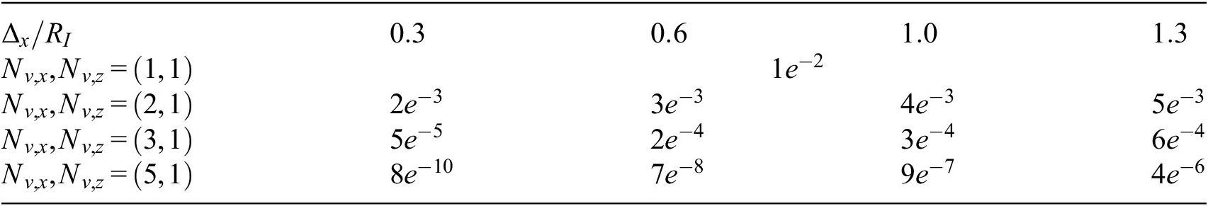
C. KPF initializations
We discuss here the initialization of the KPF particles. To mitigate 1, 2, 3, and 5, we assume that we know a priori the number of vortices ![]() but we know neither
but we know neither ![]() nor
nor ![]() . Thus, to initialize a particle, we randomly choose a value of
. Thus, to initialize a particle, we randomly choose a value of ![]() uniformly in
uniformly in ![]() , we choose randomly
, we choose randomly ![]() longitudinal positions so that
longitudinal positions so that ![]() and we choose randomly
and we choose randomly ![]() transverse positions, uniformly in
transverse positions, uniformly in ![]() . In Table C1, we compute the probability for a particle to be initialized as the real gust vortices with an uncertainty on the position of one chord and a 10% uncertainty on the circulation. Table C1 shows that the probability for a particle to be initialized as the gust vortices decreases very sharply as
. In Table C1, we compute the probability for a particle to be initialized as the real gust vortices with an uncertainty on the position of one chord and a 10% uncertainty on the circulation. Table C1 shows that the probability for a particle to be initialized as the gust vortices decreases very sharply as ![]() increases and this probability is larger for high
increases and this probability is larger for high ![]() than for low
than for low ![]() . This is due to our constraint on the longitudinal positions,
. This is due to our constraint on the longitudinal positions, ![]() is s.t.
is s.t. ![]() .
.
We also examine the choice of measurement noise ![]() . First, we observe experimentally that
. First, we observe experimentally that ![]() varies from
varies from ![]() to
to ![]() . Consequently, a constant value of
. Consequently, a constant value of ![]() is not appropriate here, because if
is not appropriate here, because if ![]() , the KPF is unable to discriminate particles when
, the KPF is unable to discriminate particles when ![]() and, conversely, if
and, conversely, if ![]() , the KPF over-constrains the particles when
, the KPF over-constrains the particles when ![]() . We therefore propose an adaptive measurement noise to take account of this wide range of
. We therefore propose an adaptive measurement noise to take account of this wide range of ![]() values.
values.

Figure D1. Reconstruction of ![]() performed by the KPF controller.
performed by the KPF controller.
D. Estimation of the gust vortex transverse positions
We discuss here the reconstruction of ![]() performed by the KPF for 2 and 3. In Figure D1, we present the KPF reconstruction of
performed by the KPF for 2 and 3. In Figure D1, we present the KPF reconstruction of ![]() for 2 (Figure D1a) and for 3 (Figure D1b) for
for 2 (Figure D1a) and for 3 (Figure D1b) for ![]() . We compare
. We compare ![]() (
(![]() ),
), ![]() (
(![]() ),
), ![]() (
(![]() ) with the KPF estimates
) with the KPF estimates ![]() (
(![]() ),
), ![]() (
(![]() ),
), ![]() (
(![]() ). It results that the estimation of the vortex transverse positions is a more challenging task than the estimation of the vortex longitudinal positions. As a matter of fact, Figure D1 shows that for both 2 and 3, the KPF is not able to accurately track the transverse positions. It is important to note that the transverse distances between the gust vortices and the LE are, most of the time, negligible compared to the longitudinal distances. We can therefore assume that the KPF is not able to estimate them because they have a limited impact on
). It results that the estimation of the vortex transverse positions is a more challenging task than the estimation of the vortex longitudinal positions. As a matter of fact, Figure D1 shows that for both 2 and 3, the KPF is not able to accurately track the transverse positions. It is important to note that the transverse distances between the gust vortices and the LE are, most of the time, negligible compared to the longitudinal distances. We can therefore assume that the KPF is not able to estimate them because they have a limited impact on ![]() compared to their longitudinal counterpart (Eq. 5).
compared to their longitudinal counterpart (Eq. 5).

Figure E1. The normalized lift coefficients ![]() (left) and the normalized control laws
(left) and the normalized control laws ![]() (right) under the OL controller - - -, the FO controller
(right) under the OL controller - - -, the FO controller ![]() , control free - - for 1 with
, control free - - for 1 with ![]() . Solid lines represent the averaged quantities and colored areas represent the associated standard deviations, and the gray area on the
. Solid lines represent the averaged quantities and colored areas represent the associated standard deviations, and the gray area on the ![]() -axis indicates the presence of the gust vortex on the profile.
-axis indicates the presence of the gust vortex on the profile.
E. Comparison with thin airfoil theory based control
In the limit of thin airfoil theory, the lift coefficient in the control free configuration, ![]() , can be viewed as the lift response to a perturbation in AoA
, can be viewed as the lift response to a perturbation in AoA ![]() , such that
, such that ![]() . In the most simple quasi-steady framework,
. In the most simple quasi-steady framework, ![]() can thus be mitigated by applying a control law that opposes
can thus be mitigated by applying a control law that opposes ![]() , i.e.
, i.e. ![]() . This rough approximation assumes that (i) the pitch motion does not affect the trajectories and the circulations of the gust and wake vortices and, (ii) neglects the unsteady effects. In the following, we refer to the open-loop (OL) controller defined as
. This rough approximation assumes that (i) the pitch motion does not affect the trajectories and the circulations of the gust and wake vortices and, (ii) neglects the unsteady effects. In the following, we refer to the open-loop (OL) controller defined as ![]() as the OL controller. Note that this controller is only introduced for analysis purposes since
as the OL controller. Note that this controller is only introduced for analysis purposes since ![]() is not known a priori. To compare the difference between the
is not known a priori. To compare the difference between the ![]() -FO controller and the OL controller, we display in Figure E1 the FO control laws, the OL control laws and their associated lift coefficients when the controllers undergo 1 with
-FO controller and the OL controller, we display in Figure E1 the FO control laws, the OL control laws and their associated lift coefficients when the controllers undergo 1 with ![]() . Figure E1 shows that for
. Figure E1 shows that for ![]() , there is a good agreement between the two control laws. However, for higher
, there is a good agreement between the two control laws. However, for higher ![]() , the FO controller differs from the OL controller. This differences involve a poor mitigation of the OL controller and a good mitigation of the FO controller. These observations must be seen in the context of the assumptions made to derive the OL controller. We assume that the pitch motion does not induce a high amplitude
, the FO controller differs from the OL controller. This differences involve a poor mitigation of the OL controller and a good mitigation of the FO controller. These observations must be seen in the context of the assumptions made to derive the OL controller. We assume that the pitch motion does not induce a high amplitude ![]() but under OL control, this assumption is not valid for
but under OL control, this assumption is not valid for ![]() . Furthermore, we assume that there is no coupling between the pitching motion and the wake vortices, however, in the ideal case where the FO controller maintains the lift coefficient at
. Furthermore, we assume that there is no coupling between the pitching motion and the wake vortices, however, in the ideal case where the FO controller maintains the lift coefficient at ![]() , the wake vortices have zero circulation. This result shows the great capability of DRL to build efficient controllers without the need of assumptions or simplifications of the physics, as done for the OL controller.
, the wake vortices have zero circulation. This result shows the great capability of DRL to build efficient controllers without the need of assumptions or simplifications of the physics, as done for the OL controller.
F. All control laws for 2
In Section 5.3, we observe that the KPF controller exhibits noisy actuation for gust f(2). To better understand the reasons behind this behavior, Figure F1 displays the five KPF and FO controllers used for the visualizations in Section 5.3. The results show that only one out of the five controllers demonstrates this noisy actuation behavior. We therefore conclude that the noisy actuation is caused by variability within the control functions.

Figure F1. All control laws used for Figure 11-g. ![]() ,
, ![]() respectively represent
respectively represent ![]() under
under ![]() -FO control and
-FO control and ![]() -KPF control, when the controllers undergo 2 with
-KPF control, when the controllers undergo 2 with ![]() . The results have been computed for
. The results have been computed for ![]() . Solid lines represent the average control laws, and the colored areas are the associated standard deviations.
. Solid lines represent the average control laws, and the colored areas are the associated standard deviations.


 Open access
Comments
No Comments have been published for this article.