


1 Introduction
Calabi–Weil local rigidity [Reference CalabiCal61, Reference WeilWei62] (an important precursor to Mostow [Reference MostowMos73] rigidity) states that, for $n \geq 3$
, the action of the fundamental group of a hyperbolic n-manifold by conformal maps on the boundary sphere
$n \geq 3$
, the action of the fundamental group of a hyperbolic n-manifold by conformal maps on the boundary sphere $S^{n-1}$
is locally rigid: any nearby conformal action is conjugate in
$S^{n-1}$
is locally rigid: any nearby conformal action is conjugate in $SO^+(n, 1)$
to the original action. Inspired by this, we investigate rigidity for the actions on boundary spheres of the broader class of all Gromov hyperbolic groups with sphere boundary. These boundaries do not typically admit a natural conformal or even a
$SO^+(n, 1)$
to the original action. Inspired by this, we investigate rigidity for the actions on boundary spheres of the broader class of all Gromov hyperbolic groups with sphere boundary. These boundaries do not typically admit a natural conformal or even a $C^1$
structure, so the relevant notion of local stability is that from topological dynamics. Recall that an action
$C^1$
structure, so the relevant notion of local stability is that from topological dynamics. Recall that an action $\rho _0 \colon \thinspace G \to \mathrm {Homeo}(X)$
of a group G on a topological space X is a topological factor of an action
$\rho _0 \colon \thinspace G \to \mathrm {Homeo}(X)$
of a group G on a topological space X is a topological factor of an action $\rho \colon \thinspace G \to \mathrm {Homeo}(Y)$
if there is a surjective, continuous map
$\rho \colon \thinspace G \to \mathrm {Homeo}(Y)$
if there is a surjective, continuous map $h\colon \thinspace Y \to X$
, such that
$h\colon \thinspace Y \to X$
, such that $h \circ \rho = \rho _0 \circ h$
. Such a map h is called a semiconjugacy. An action of a group G on a topological space X is topologically stable or
$h \circ \rho = \rho _0 \circ h$
. Such a map h is called a semiconjugacy. An action of a group G on a topological space X is topologically stable or $C^0$
stable if it is a factor of any sufficiently close action in the compact-open topology on
$C^0$
stable if it is a factor of any sufficiently close action in the compact-open topology on $\mathrm {Hom}(G, \mathrm {Homeo}(X))$
. We prove the following.
$\mathrm {Hom}(G, \mathrm {Homeo}(X))$
. We prove the following.
Theorem 1.1 (Topological stability)
Let G be a hyperbolic group with sphere boundary. Then the action of G on $\partial G$
is topologically stable. More precisely, given any neighborhood V of the identity in the space of continuous self-maps of
$\partial G$
is topologically stable. More precisely, given any neighborhood V of the identity in the space of continuous self-maps of $S^n$
, there exists a neighborhood U of the standard boundary action in
$S^n$
, there exists a neighborhood U of the standard boundary action in $\mathrm {Hom}(G, \mathrm {Homeo}(S^n))$
, such that any representation in U has
$\mathrm {Hom}(G, \mathrm {Homeo}(S^n))$
, such that any representation in U has $\rho _0$
as a factor, with semiconjugacy contained in V.
$\rho _0$
as a factor, with semiconjugacy contained in V.
In parallel with Calabi–Weil rigidity, this says that these boundary actions exhibit the strongest possible form of local rigidity. While there is overlap in the groups considered (fundamental groups of closed hyperbolic manifolds are Gromov hyperbolic), our result is neither a special case nor a generalization of the classical case. We consider a much broader space of deformations – actions by homeomorphisms rather than conformal maps – but semiconjugacy is of course weaker than conformal conjugacy, which one cannot hope for when considering general continuous deformations (see, in particular, the examples of [Reference Bowden and MannBM19, Section 4]).
History and related results
“Stability from hyperbolicity” is an important and recurring theme in dynamical systems. For instance, hyperbolic (Anosov) diffeomorphisms are topologically stable, thanks to the well known shadowing lemma. However, in much of the existing literature, hyperbolicity is described using some smooth or at least $C^1$
structure, while the actions we consider are typically not differentiable, only having Hölder regularity.
$C^1$
structure, while the actions we consider are typically not differentiable, only having Hölder regularity.
Regarding boundary actions of groups, Sullivan’s 1985 Structural stability implies hyperbolicity for Kleinian groups [Reference SullivanSul85], characterizes convex-cocompact subgroups of $\mathrm {PSL}(2,\mathbb {C})$
as those subgroups whose action on their limit set is stable under
$\mathrm {PSL}(2,\mathbb {C})$
as those subgroups whose action on their limit set is stable under $C^1$
perturbations. Sullivan uses the fact that group elements expand neighborhoods of points to produce a coding of orbits that is insensitive to perturbation. This technique was recently generalized by Kapovich–Kim–Lee [Reference Kapovich, Kim and LeeKKL] to a much broader setting, including Lipschitz perturbations of many group actions on metric spaces which satisfy a generalized version of Sullivan’s expansivity condition.
$C^1$
perturbations. Sullivan uses the fact that group elements expand neighborhoods of points to produce a coding of orbits that is insensitive to perturbation. This technique was recently generalized by Kapovich–Kim–Lee [Reference Kapovich, Kim and LeeKKL] to a much broader setting, including Lipschitz perturbations of many group actions on metric spaces which satisfy a generalized version of Sullivan’s expansivity condition.
Matsumoto [Reference MatsumotoMat87] gives a more robust form of rigidity for the actions of fundamental groups of compact surfaces on their boundary at infinity. In this case, the boundary is a topological circle, and Matsumoto’s work implies that any deformation of such a boundary action is semiconjugate to the original action. Motivated by this, Bowden and the first author [Reference Bowden and MannBM19] studied the actions of the fundamental groups of compact Riemannian manifolds on their boundaries at infinity, showing these satisfy a form of local rigidity. Again hyperbolicity played a role, this time in the form of the Anosov property of geodesic flow on such negatively curved manifolds. Theorem 1.1 generalizes aspects of both Sullivan’s and Matsumoto’s program. While hyperbolic groups acting on their boundaries are among the examples studied by Kapovich–Kim–Lee, their methods only apply to perturbations which continue to have Sullivan’s expansivity, for instance, Lipschitz-close actions. General $C^0$
perturbations need not be Lipschitz close, so Sullivan’s coding no longer applies, and we need an entirely new method of proof. Our strategy is more in the spirit of [Reference Bowden and MannBM19] but uses large-scale geometry in place of the Riemannian manifold structure and Anosov geodesic flow.
$C^0$
perturbations need not be Lipschitz close, so Sullivan’s coding no longer applies, and we need an entirely new method of proof. Our strategy is more in the spirit of [Reference Bowden and MannBM19] but uses large-scale geometry in place of the Riemannian manifold structure and Anosov geodesic flow.
Our focus on spheres is motivated in part by the fact that these are the most homogeneous group boundaries. At the other end of the spectrum, Kapovich and Kleiner [Reference Kapovich and KleinerKK00] constructed hyperbolic groups that are boundary rigid, in the sense that any homeomorphism of the boundary comes from the action of an element of the group. These groups trivially satisfy local rigidity, since $\mathrm {Homeo}(\partial G) \cong G$
is discrete. By contrast, homeomorphisms of the sphere are very easy to perturb, each having an infinite dimensional family of deformations. The reader may consult [Reference Coornaert and PapadopoulosCP93] or [Reference Kapovich and BenakliKB02] for more background on the dynamics of hyperbolic groups acting on their boundaries.
$\mathrm {Homeo}(\partial G) \cong G$
is discrete. By contrast, homeomorphisms of the sphere are very easy to perturb, each having an infinite dimensional family of deformations. The reader may consult [Reference Coornaert and PapadopoulosCP93] or [Reference Kapovich and BenakliKB02] for more background on the dynamics of hyperbolic groups acting on their boundaries.
Scope
Bartels, Lück and Weinberger [Reference Bartels, Lück and WeinbergerBLW10, Example 5.2] give, for all $k\geq 2$
, examples of torsion-free hyperbolic groups G with
$k\geq 2$
, examples of torsion-free hyperbolic groups G with $\partial G = S^{4k-1}$
that are not the fundamental group of any smooth, closed, aspherical manifold (note that such an example with
$\partial G = S^{4k-1}$
that are not the fundamental group of any smooth, closed, aspherical manifold (note that such an example with $\partial G = S^2$
would give a counterexample to the Cannon Conjecture). These examples show that, even in the torsion free case, Theorem 1.1 is a strict generalization of the work of [Reference Bowden and MannBM19] on Riemannian manifold fundamental groups. Of course, groups with torsion provide numerous other examples, and the tools introduced within the large scale geometric framework of the proof should be of independent interest.
$\partial G = S^2$
would give a counterexample to the Cannon Conjecture). These examples show that, even in the torsion free case, Theorem 1.1 is a strict generalization of the work of [Reference Bowden and MannBM19] on Riemannian manifold fundamental groups. Of course, groups with torsion provide numerous other examples, and the tools introduced within the large scale geometric framework of the proof should be of independent interest.
Outline
The broad strategy of the proof is to translate the data of a G–action on $S^n$
into a G–action on a sphere bundle over a particular space quasi-isometric to G, then show that nearby actions can be related by a G-equivariant map between their respective bundles that is close to the identity on large compact sets. This lets us promote metrically stable notions in coarse negative curvature (such as the property of a subset being bounded Hausdorff distance from a geodesic) into stability for the group action.
$S^n$
into a G–action on a sphere bundle over a particular space quasi-isometric to G, then show that nearby actions can be related by a G-equivariant map between their respective bundles that is close to the identity on large compact sets. This lets us promote metrically stable notions in coarse negative curvature (such as the property of a subset being bounded Hausdorff distance from a geodesic) into stability for the group action.
In Section 2, we collect general results and preliminary lemmas on hyperbolic metric spaces. In Section 3, we construct the bundles and equivariant map advertised above, in the broader context of (not necessarily hyperbolic) groups acting on manifolds, which is the natural setting for this technique.
To apply this technique to the proof of Theorem 1.1, we need to find a suitably nice space X with a proper, free, cocompact action of G by isometries. If G is torsion free, the space of distinct triples in $\partial G$
is a natural choice, but if G has torsion, the action of G on triples may not be free. We remedy this in Sections 4 and 5, first reducing to the case where G acts faithfully on
$\partial G$
is a natural choice, but if G has torsion, the action of G on triples may not be free. We remedy this in Sections 4 and 5, first reducing to the case where G acts faithfully on $\partial G$
, and then showing that one may remove a small neighborhood of the space of fixed boundary triples without losing too much geometry, giving a suitable space to use in the rest of the proof. We also prove several technical lemmas on the triple space for reference in later sections.
$\partial G$
, and then showing that one may remove a small neighborhood of the space of fixed boundary triples without losing too much geometry, giving a suitable space to use in the rest of the proof. We also prove several technical lemmas on the triple space for reference in later sections.
Section 6 sets up the main proof and specifies a neighborhood of the boundary action where Theorem 1.1 holds. The bundles from Section 3 come with natural topological foliations, and Section 6.2 shows that the image of one of these foliations in the source space (whose leaves are parameterized by points of $\partial G$
) intersects leaves in the target along coarsely geodesic sets. Section 7 shows that the endpoints of these coarse geodesics depend only on the original leaf, thus giving a map h from the leaf space of one foliation to the Gromov boundary of X. Both the leaf space and the Gromov boundary of X are canonically homeomorphic to
$\partial G$
) intersects leaves in the target along coarsely geodesic sets. Section 7 shows that the endpoints of these coarse geodesics depend only on the original leaf, thus giving a map h from the leaf space of one foliation to the Gromov boundary of X. Both the leaf space and the Gromov boundary of X are canonically homeomorphic to $\partial G$
, and the map h is our semiconjugacy.
$\partial G$
, and the map h is our semiconjugacy.
2 Background
We set notation, collect some general results on hyperbolic metric spaces, and prove some preliminary lemmas needed for the main theorem.
2.1 Setup
We fix the following notation. G denotes a nonelementary hyperbolic group; in this section, we do not require $\partial G$
to be a sphere. We fix a generating set
$\partial G$
to be a sphere. We fix a generating set $\mathcal {S}$
, which gives us a Cayley graph
$\mathcal {S}$
, which gives us a Cayley graph $\Gamma $
and metric
$\Gamma $
and metric $d_{\Gamma }$
on
$d_{\Gamma }$
on $\Gamma $
. Vertices of
$\Gamma $
. Vertices of $\Gamma $
are identified with group elements. In particular, the identity
$\Gamma $
are identified with group elements. In particular, the identity $\mathbf {e}$
is a vertex of
$\mathbf {e}$
is a vertex of $\Gamma $
. The metric
$\Gamma $
. The metric $d_{\Gamma }$
is
$d_{\Gamma }$
is $\nu $
–hyperbolic (in the sense that geodesic triangles are
$\nu $
–hyperbolic (in the sense that geodesic triangles are $\nu $
–thin) for some
$\nu $
–thin) for some $\nu>0$
. We will fix a constant
$\nu>0$
. We will fix a constant $\delta \ge \nu $
with some other convenient properties later. The Gromov boundary of the group is denoted
$\delta \ge \nu $
with some other convenient properties later. The Gromov boundary of the group is denoted $\partial G$
, this is of course equal to the Gromov boundary of
$\partial G$
, this is of course equal to the Gromov boundary of $\Gamma $
.
$\Gamma $
.
We write $({x}\,|\,{y})_{z}$
for the Gromov product of x and y at z. The point z must lie in
$({x}\,|\,{y})_{z}$
for the Gromov product of x and y at z. The point z must lie in $\Gamma $
, but
$\Gamma $
, but $x,y$
may be in
$x,y$
may be in $\Gamma \cup \partial G$
, using the standard definition of the Gromov product at infinity (see e.g. [Reference Bridson and HaefligerBH99, III.H.3.15]), as follows:
$\Gamma \cup \partial G$
, using the standard definition of the Gromov product at infinity (see e.g. [Reference Bridson and HaefligerBH99, III.H.3.15]), as follows:
 $$\begin{align*}({x}\,|\,{y})_{p} = \sup\left\{\left. \liminf_{i,j\to \infty} ({x_i}\,|\,{y_j})_{p}\ \right|\ \lim_{i\to\infty} x_i = x, \lim_{i\to\infty}y_i =y\right\}.\end{align*}$$
We also fix a visual metric $d_{\mathrm {vis}}$
on
$d_{\mathrm {vis}}$
on $\partial G$
. This means a metric so that there are constants
$\partial G$
. This means a metric so that there are constants $\lambda>1$
and
$\lambda>1$
and $k_2>k_1>0$
satisfying, for all
$k_2>k_1>0$
satisfying, for all $a,b\in \partial G$
,
$a,b\in \partial G$
,
 $$ \begin{align} k_1 \lambda^{-({a}\,|\,{b})_{\mathbf{e}}}\le d_{\mathrm{vis}}(a,b)\le k_2\lambda^{-({a}\,|\,{b})_{\mathbf{e}}} \end{align} $$
(see [Reference Bridson and HaefligerBH99, III.H.3] or [Reference Ghys and de la HarpeGdlH90, 7.3] for more details, including the existence of such a metric). Unless otherwise specified, all metric notions in $\partial G$
(such as balls
$\partial G$
(such as balls $B_r(p)$
) will be defined using this visual metric. Occasionally, when specializing to
$B_r(p)$
) will be defined using this visual metric. Occasionally, when specializing to $\partial G = S^n$
, we also make use of the standard round metric on
$\partial G = S^n$
, we also make use of the standard round metric on $S^n$
.
$S^n$
.
We will need to use the following lemma for estimating the Gromov product of points at infinity in a $\nu $
-hyperbolic space.
$\nu $
-hyperbolic space.
Lemma 2.1. Let M be $\nu $
–hyperbolic, and let
$\nu $
–hyperbolic, and let $p\in M$
. Let
$p\in M$
. Let $\alpha ,\beta \in \partial M$
be represented by geodesic rays
$\alpha ,\beta \in \partial M$
be represented by geodesic rays $\gamma _\alpha ,\gamma _\beta $
starting at p. For any points
$\gamma _\alpha ,\gamma _\beta $
starting at p. For any points $a\in \gamma _\alpha , b\in \gamma _\beta $
,
$a\in \gamma _\alpha , b\in \gamma _\beta $
,
 $$\begin{align*}({\alpha}\,|\,{\beta})_{p}\ge ({a}\,|\,{b})_{p} - 2\nu.\end{align*}$$
Proof. From the definition of Gromov product at infinity, it follows that
 $$\begin{align*}({\alpha}\,|\,{\beta})_{p} \ge \liminf_{s,t\to\infty} ({\gamma_\alpha(s)}\,|\,{\gamma_\beta(t)})_{p}.\end{align*}$$
To simplify notation, consider p as a base point and write $|\cdot |$
for
$|\cdot |$
for $d_M(p,\cdot )$
. Suppose that c is a point on
$d_M(p,\cdot )$
. Suppose that c is a point on $\gamma _\alpha $
and d a point on
$\gamma _\alpha $
and d a point on $\gamma _\beta $
so that
$\gamma _\beta $
so that $|c|>|a|$
and
$|c|>|a|$
and $|d|>|b|$
. We want to show that
$|d|>|b|$
. We want to show that $({c}\,|\,{d})_{p} \ge ({a}\,|\,{b})_{p} - 2\nu $
.
$({c}\,|\,{d})_{p} \ge ({a}\,|\,{b})_{p} - 2\nu $
.
Consider the triple of Gromov products $({c}\,|\,{d})_{p}$
,
$({c}\,|\,{d})_{p}$
, $({b}\,|\,{d})_{p} = |b|$
, and
$({b}\,|\,{d})_{p} = |b|$
, and $({c}\,|\,{b})_{p}\le |b|$
. As is well known, it follows from
$({c}\,|\,{b})_{p}\le |b|$
. As is well known, it follows from $\nu $
–hyperbolicity that any one of such a triple is bounded below by
$\nu $
–hyperbolicity that any one of such a triple is bounded below by $\nu $
less than the minimum of the other two, so we have
$\nu $
less than the minimum of the other two, so we have
 $$ \begin{align} ({c}\,|\,{d})_{p} \ge ({c}\,|\,{b})_{p} - \nu.\end{align} $$
Considering next the triple $({c}\,|\,{b})_{p}$
,
$({c}\,|\,{b})_{p}$
, $({c}\,|\,{a})_{p} = |a|$
, and
$({c}\,|\,{a})_{p} = |a|$
, and $({a}\,|\,{b})_{p} \le |a|$
, we conclude
$({a}\,|\,{b})_{p} \le |a|$
, we conclude
 $$ \begin{align} ({c}\,|\,{b})_{p} \ge ({a}\,|\,{b})_{p} - \nu.\end{align} $$
Together (2) and (3) give $({c}\,|\,{d})_{p} \ge ({a}\,|\,{b})_{p} - 2\nu $
, as desired.
$({c}\,|\,{d})_{p} \ge ({a}\,|\,{b})_{p} - 2\nu $
, as desired.
2.2 The space of triples
Write $\Xi $
for the space of ordered distinct triples of points in the Gromov boundary
$\Xi $
for the space of ordered distinct triples of points in the Gromov boundary $\partial \Gamma = \partial G$
. We use the following well known property.
$\partial \Gamma = \partial G$
. We use the following well known property.
Proposition 2.2 (Convergence group property (see [Reference BowditchBow98, Reference TukiaTuk98] and [Reference GromovGro87] Section 8.2.M))
G acts properly discontinuously and cocompactly on $\Xi $
, and each point
$\Xi $
, and each point $a \in \partial G$
is a conical limit point, meaning that there exists
$a \in \partial G$
is a conical limit point, meaning that there exists $\{g_i\}_{i\in \mathbb {N}}\subset G$
and
$\{g_i\}_{i\in \mathbb {N}}\subset G$
and $p \neq q \in \partial G $
, such that
$p \neq q \in \partial G $
, such that $g_i(a) \to p$
and
$g_i(a) \to p$
and $g_i(z) \to q$
for all
$g_i(z) \to q$
for all $z \in \partial G - \{a\}$
.
$z \in \partial G - \{a\}$
.
The following definition can be thought of as giving a coarse projection map from $\Xi $
to
$\Xi $
to $\Gamma $
(compare [Reference GromovGro87, Section 8.2.K]). When S is a subset of a metric space, we use the notation
$\Gamma $
(compare [Reference GromovGro87, Section 8.2.K]). When S is a subset of a metric space, we use the notation $N_r(S)$
to indicate the open r–neighborhood of S.
$N_r(S)$
to indicate the open r–neighborhood of S.
Definition 2.3 (Coarse projection)
For each $r>0$
, we define a projection map
$r>0$
, we define a projection map $\pi _r$
from
$\pi _r$
from $\Xi $
to subgraphs of
$\Xi $
to subgraphs of $\Gamma $
as follows. For
$\Gamma $
as follows. For $(a,b,c)\in \Xi $
, let
$(a,b,c)\in \Xi $
, let $\mathcal {G}(a,b,c)$
be the set of geodesics in
$\mathcal {G}(a,b,c)$
be the set of geodesics in $\Gamma $
with endpoints in
$\Gamma $
with endpoints in $\{a,b,c\}$
. For each
$\{a,b,c\}$
. For each $r>0$
, define
$r>0$
, define $\pi _r(a,b,c) \subset \Gamma $
to be the smallest subgraph of
$\pi _r(a,b,c) \subset \Gamma $
to be the smallest subgraph of $\Gamma $
containing
$\Gamma $
containing $\bigcap _{\gamma \in \mathcal {G}(a,b,c)} N_{r-1}(\gamma ).$
If Z is a subset of $\Xi $
, we define
$\Xi $
, we define $\pi _r(Z) = \bigcup _{z \in Z} \pi _r(z)$
. For
$\pi _r(Z) = \bigcup _{z \in Z} \pi _r(z)$
. For $s\in \Gamma $
, we define
$s\in \Gamma $
, we define $\pi _r^{-1}(s) = \{(a,b,c)\mid s\in \pi (a,b,c)\}$
; for
$\pi _r^{-1}(s) = \{(a,b,c)\mid s\in \pi (a,b,c)\}$
; for $S\subset \Gamma $
, define
$S\subset \Gamma $
, define $\pi _r^{-1}(S) = \bigcup _{s\in S} \pi _r^{-1}(s)$
.
$\pi _r^{-1}(S) = \bigcup _{s\in S} \pi _r^{-1}(s)$
.
Remark 2.4. If r is sufficiently large (depending on the hyperbolicity constant of $\Gamma $
), then
$\Gamma $
), then $\pi _r(a,b,c)$
is always nonempty. Moreover, for any
$\pi _r(a,b,c)$
is always nonempty. Moreover, for any $x\in \pi _r(a,b,c)$
and any geodesic
$x\in \pi _r(a,b,c)$
and any geodesic $\gamma $
with endpoints in
$\gamma $
with endpoints in $\{a,b,c\}$
, we have
$\{a,b,c\}$
, we have $d_{\Gamma }(x,\gamma )\le r$
. We will make frequent use of this estimate.
$d_{\Gamma }(x,\gamma )\le r$
. We will make frequent use of this estimate.
Lemma 2.5. For every $r\ge 0$
, there is a
$r\ge 0$
, there is a $Q(r) \ge 0$
so
$Q(r) \ge 0$
so $\mathrm {diam}(\pi _r(a,b,c))\le Q(r)$
for all
$\mathrm {diam}(\pi _r(a,b,c))\le Q(r)$
for all $(a,b,c)\in \Xi $
.
$(a,b,c)\in \Xi $
.
Proof. Recall $\Gamma $
is
$\Gamma $
is $\nu $
–hyperbolic, meaning that triangles are
$\nu $
–hyperbolic, meaning that triangles are $\nu $
–thin. Let
$\nu $
–thin. Let $(a,b,c) \in X$
be given. Fix biinfinite geodesics
$(a,b,c) \in X$
be given. Fix biinfinite geodesics $[a,b], [b,c]$
, and
$[a,b], [b,c]$
, and $[a,c]$
in
$[a,c]$
in $\Gamma $
. Approximate this ideal triangle by a triangle in
$\Gamma $
. Approximate this ideal triangle by a triangle in $\Gamma $
by choosing points
$\Gamma $
by choosing points $a'\ b'$
and
$a'\ b'$
and $c' \in \Gamma $
on the geodesics
$c' \in \Gamma $
on the geodesics $[a,b], [b,c]$
, and
$[a,b], [b,c]$
, and $[a,c]$
, respectively, satisfying
$[a,c]$
, respectively, satisfying $d_{\Gamma }(a', [a, c]) < \nu $
and
$d_{\Gamma }(a', [a, c]) < \nu $
and $d_{\Gamma }(a', [b, c])> r + 2 \nu $
, and such that the same two inequalities also hold when the letters
$d_{\Gamma }(a', [b, c])> r + 2 \nu $
, and such that the same two inequalities also hold when the letters $a, b, c$
are cyclically permuted. Then
$a, b, c$
are cyclically permuted. Then $\pi _r(a,b,c)$
is a subset of
$\pi _r(a,b,c)$
is a subset of
 $$\begin{align*}S_r := N_{r + \nu}([a',b']) \cap N_{r + \nu}([b',c']) \cap N_{r + \nu}([c',a']) \end{align*}$$
so it suffices to show this set has diameter bounded by $Q(r)$
, for some suitable function Q.
$Q(r)$
, for some suitable function Q.
Let p denote the map from the triangle with sides $[a',b'], [b', c']$
, and
$[a',b'], [b', c']$
, and $[a', c']$
to a tripod witnessing that the triangle is
$[a', c']$
to a tripod witnessing that the triangle is $\nu $
–thin, and let Z be the preimage of the center, this is a set of three points with diameter at most
$\nu $
–thin, and let Z be the preimage of the center, this is a set of three points with diameter at most $\nu $
. We now claim that
$\nu $
. We now claim that $S_r$
lies in the
$S_r$
lies in the $3r + 5 \nu $
-neighborhood of Z, which is enough to prove the lemma. To prove the claim, suppose
$3r + 5 \nu $
-neighborhood of Z, which is enough to prove the lemma. To prove the claim, suppose $s \in S_r$
, so there exist points
$s \in S_r$
, so there exist points $x_1, x_2$
, and
$x_1, x_2$
, and $x_3$
on
$x_3$
on $[a',b'], [b', c']$
, and
$[a',b'], [b', c']$
, and $[a', c']$
, respectively, with
$[a', c']$
, respectively, with $d_{\Gamma }(x_i, s) < r + \nu $
. Then for any
$d_{\Gamma }(x_i, s) < r + \nu $
. Then for any $i = 1, 2, 3$
, there exists some j so that
$i = 1, 2, 3$
, there exists some j so that $p(x_i)$
and
$p(x_i)$
and $p(x_j)$
lie on different prongs of the tripod, so there is a path between them passing through the midpoint m of the tripod. Thus, we have
$p(x_j)$
lie on different prongs of the tripod, so there is a path between them passing through the midpoint m of the tripod. Thus, we have
 $$\begin{align*}d_{\Gamma}(x_i, Z) = d_{\Gamma}(p(x_i), m) \leq d_{\Gamma}(p(x_i), p(x_j)) \leq d_{\Gamma}(x_i, x_j) + 2 \nu \leq 2r + 4 \nu ,\end{align*}$$
where the last inequality follows from the fact that $d_{\Gamma }(x_i, s) < r + \nu $
. This proves the claim.
$d_{\Gamma }(x_i, s) < r + \nu $
. This proves the claim.
Lemma 2.6. Let $r\ge 0$
. For any compact
$r\ge 0$
. For any compact $K\subset \Xi $
, the set
$K\subset \Xi $
, the set $\pi _r(K)$
is bounded.
$\pi _r(K)$
is bounded.
Proof. Let $K\subset \Xi $
be compact. Increasing r makes
$K\subset \Xi $
be compact. Increasing r makes $\pi _r(K)$
larger. Using Remark 2.4, we can therefore assume that for every
$\pi _r(K)$
larger. Using Remark 2.4, we can therefore assume that for every $(a,b,c)$
, there is some
$(a,b,c)$
, there is some $x\in \pi _r(a,b,c)$
.
$x\in \pi _r(a,b,c)$
.
For each $(a,b,c)\in K$
, there is an open neighborhood U of
$(a,b,c)\in K$
, there is an open neighborhood U of $(a,b,c)$
in
$(a,b,c)$
in $\Xi $
, such that, for each point
$\Xi $
, such that, for each point $(u, v, w) \in U$
, any geodesics joining points in
$(u, v, w) \in U$
, any geodesics joining points in $\{u,v,w\}$
come within
$\{u,v,w\}$
come within $2 \nu + r$
of the point x. In particular,
$2 \nu + r$
of the point x. In particular, $x\in \pi _{r+2\nu }(u,v,w)$
. If
$x\in \pi _{r+2\nu }(u,v,w)$
. If $y\in \pi _r(u,v,w)$
, then
$y\in \pi _r(u,v,w)$
, then $d_{\Gamma }(x,y)\le Q(r+2\nu )$
, so
$d_{\Gamma }(x,y)\le Q(r+2\nu )$
, so $\pi _r(U)$
has diameter at most
$\pi _r(U)$
has diameter at most $2 Q(r+2\nu )$
.
$2 Q(r+2\nu )$
.
By compactness, we can cover K with finitely many neighborhoods U as in the last paragraph, so $\pi _r(K)$
is bounded.
$\pi _r(K)$
is bounded.
It will be convenient to choose a hyperbolicity constant for $\Gamma $
that simultaneously satisfies several properties. The properties we use are collected in the following lemma.
$\Gamma $
that simultaneously satisfies several properties. The properties we use are collected in the following lemma.
Lemma 2.7. There exists $\delta>0$
so that all of the following hold:
$\delta>0$
so that all of the following hold:
-
(δ1) Every geodesic triangle in $\Gamma $
is
$\delta $
–thin.
$\Gamma $
is
$\delta $
–thin. -
(δ2) Every geodesic bigon or triangle with vertices in
$\Gamma \cup \partial G$
is
$\delta $
–slim. -
(δ3) For any point
$p\in \Gamma $
, and any
$a,b,c\in \Gamma \cup \partial G$
,
$$\begin{align*}({a}\,|\,{b})_{p}\ge \min\{({a}\,|\,{c})_{p},({b}\,|\,{c})_{p}\}-\delta.\end{align*}$$
-
(δ4) For all
$p\in \Gamma $
,
$\pi _\delta ^{-1}(p)$
is nonempty. -
(δ5) The set
$\pi _\delta (\{a\}\times \{b\}\times (\partial G-\{a,b\}))$
contains every geodesic joining a to b.


Proof. Since $\Gamma $
is
$\Gamma $
is $\nu $
–hyperbolic, items (δ1) and (δ2) hold for any
$\nu $
–hyperbolic, items (δ1) and (δ2) hold for any $\delta \ge 2\nu $
. For item (δ3), see [Reference Bridson and HaefligerBH99, III.H.3.17.(4)]. Item (δ4) follows from G-equivariance and the fact that
$\delta \ge 2\nu $
. For item (δ3), see [Reference Bridson and HaefligerBH99, III.H.3.17.(4)]. Item (δ4) follows from G-equivariance and the fact that $\pi _\delta (a,b,c)$
is nonempty when
$\pi _\delta (a,b,c)$
is nonempty when $\delta $
is large enough. For (δ5), suppose we are given a point z on a geodesic
$\delta $
is large enough. For (δ5), suppose we are given a point z on a geodesic $\gamma $
joining a and b, take
$\gamma $
joining a and b, take $c \in \partial G$
minimizing
$c \in \partial G$
minimizing $\max \{({a}\,|\,{c})_{z}, ({b}\,|\,{c})_{z} \}$
. Cocompactness of the action of G allows one to bound this minimum from above, independently of
$\max \{({a}\,|\,{c})_{z}, ({b}\,|\,{c})_{z} \}$
. Cocompactness of the action of G allows one to bound this minimum from above, independently of $a, b$
, and c, and this can be used to give an upper bound on the distance from z to any geodesic joining a or b with c.
$a, b$
, and c, and this can be used to give an upper bound on the distance from z to any geodesic joining a or b with c.
Notation 2.8. For the rest of the paper, we fix some $\delta>0$
so the conclusions of Lemma 2.7 hold, and denote the coarse projection
$\delta>0$
so the conclusions of Lemma 2.7 hold, and denote the coarse projection $\pi _\delta $
by
$\pi _\delta $
by $\pi $
.
$\pi $
.
Definition 2.9 (Minimum separation)
For $x = (a,b,c)\in \Xi $
, we define
$x = (a,b,c)\in \Xi $
, we define
 $$\begin{align*}\mathrm{minsep}(x) = \min\{d_{\mathrm{vis}}(a,b),d_{\mathrm{vis}}(a,c),d_{\mathrm{vis}}(b,c)\}.\end{align*}$$
Notice that $1/\mathrm {minsep}$
is a proper function on X, so
$1/\mathrm {minsep}$
is a proper function on X, so $\mathrm {minsep}$
is bounded away from zero on any compact set. For a subset
$\mathrm {minsep}$
is bounded away from zero on any compact set. For a subset $D\subset \Xi $
, we define
$D\subset \Xi $
, we define $\mathrm {minsep}(D) = \inf \{\mathrm {minsep}(x)\mid x\in D\}$
.
$\mathrm {minsep}(D) = \inf \{\mathrm {minsep}(x)\mid x\in D\}$
.
2.3 A criterion for a set to be close to a geodesic
The following lemma gives a criterion for a piecewise geodesic curve to be close to a geodesic. There are various similar statements in the literature (e.g. [Reference MinasyanMin05, Lemma 4.2], [Reference Bridson and HaefligerBH99, Section III.H.1.13]), but this form will be convenient for us. We use it to prove Lemma 2.12 which is the main technical ingredient of this section.
Lemma 2.10. Let X be a $\delta $
–hyperbolic geodesic metric space, and let
$\delta $
–hyperbolic geodesic metric space, and let $l>0$
. Suppose that c is a piecewise geodesic in X made of segments of length greater than
$l>0$
. Suppose that c is a piecewise geodesic in X made of segments of length greater than $2l+8\delta $
, with Gromov products in the corners at most l. Let
$2l+8\delta $
, with Gromov products in the corners at most l. Let $\gamma $
be a geodesic with the same endpoints as c. The Hausdorff distance between
$\gamma $
be a geodesic with the same endpoints as c. The Hausdorff distance between $\gamma $
and c is at most
$\gamma $
and c is at most $l+4\delta $
.
$l+4\delta $
.
We remark that this lemma only uses $\delta $
–hyperbolicity, and not the other properties from Lemma 2.7.
$\delta $
–hyperbolicity, and not the other properties from Lemma 2.7.
Proof. A standard argument, using only the fact that $\gamma $
is a geodesic in a
$\gamma $
is a geodesic in a $\delta $
-hyperbolic space, shows that it is enough to prove c is contained in the closed
$\delta $
-hyperbolic space, shows that it is enough to prove c is contained in the closed $(l + 3\delta )$
–neighborhood of
$(l + 3\delta )$
–neighborhood of $\gamma $
. We will not give the details, as this is classical. We write c as a concatenation
$\gamma $
. We will not give the details, as this is classical. We write c as a concatenation $c_1\cdots c_k$
of geodesics, so each
$c_1\cdots c_k$
of geodesics, so each $c_i$
joins some
$c_i$
joins some $p_{i-1}$
to some
$p_{i-1}$
to some $p_i$
. The endpoints of
$p_i$
. The endpoints of $\gamma $
are
$\gamma $
are $p_0$
and
$p_0$
and $p_k$
. If
$p_k$
. If $k\le 2$
, we are done by slimness of triangles, so we assume
$k\le 2$
, we are done by slimness of triangles, so we assume $k\ge 3$
.
$k\ge 3$
.
Let x be the farthest point from $\gamma $
on c, and let
$\gamma $
on c, and let $M=d(x,\gamma )$
. Without loss of generality, we suppose that
$M=d(x,\gamma )$
. Without loss of generality, we suppose that $M>2\delta $
. It is then straightforward to show that x is within
$M>2\delta $
. It is then straightforward to show that x is within $2\delta $
of some breakpoint
$2\delta $
of some breakpoint $p_i$
(consider the triangle made up of the segment
$p_i$
(consider the triangle made up of the segment $c_i$
containing x, together with geodesics joining the endpoints of
$c_i$
containing x, together with geodesics joining the endpoints of $c_i$
to a point
$c_i$
to a point $x'\in \gamma $
closest to x).
$x'\in \gamma $
closest to x).
Since $M>2\delta $
, the breakpoint
$M>2\delta $
, the breakpoint $p_i$
cannot be either endpoint of the geodesic
$p_i$
cannot be either endpoint of the geodesic $\gamma $
; in particular,
$\gamma $
; in particular, $i\notin \{0,k\}$
. There are two cases, depending on whether or not
$i\notin \{0,k\}$
. There are two cases, depending on whether or not $i\in \{1,k-1\}$
.
$i\in \{1,k-1\}$
.
We suppose $i\notin \{1,k-1\}$
; the case
$i\notin \{1,k-1\}$
; the case $i\in \{1,k-1\}$
is similar but easier. By the assumption that segments are long,
$i\in \{1,k-1\}$
is similar but easier. By the assumption that segments are long, $d(x,\{p_{i\pm 1}\})>2l+6\delta $
. Choose a geodesic
$d(x,\{p_{i\pm 1}\})>2l+6\delta $
. Choose a geodesic $\sigma $
joining
$\sigma $
joining $p_{i-1}$
to
$p_{i-1}$
to $p_{i+1}$
. By the assumption on Gromov products in the corners, we have
$p_{i+1}$
. By the assumption on Gromov products in the corners, we have $({p_{i-1}}\,|\,{p_{i+1}})_{p_i}\le l$
. It follows that
$({p_{i-1}}\,|\,{p_{i+1}})_{p_i}\le l$
. It follows that $d(x,\sigma )\leq l+\delta $
. Let y be a closest point to
$d(x,\sigma )\leq l+\delta $
. Let y be a closest point to $p_{i-1}$
in
$p_{i-1}$
in $\gamma $
, and let z be a closest point to
$\gamma $
, and let z be a closest point to $p_{i+1}$
in
$p_{i+1}$
in $\gamma $
. Choose geodesics
$\gamma $
. Choose geodesics $[y,z]\subset \gamma $
,
$[y,z]\subset \gamma $
, $[p_{i-1},y]$
, and
$[p_{i-1},y]$
, and $[p_{i+1},z]$
. The point x lies within
$[p_{i+1},z]$
. The point x lies within $l+3\delta $
of some point w on the union of these three geodesics. We claim that
$l+3\delta $
of some point w on the union of these three geodesics. We claim that $w\in [y,z]$
, so we have
$w\in [y,z]$
, so we have $M\le l+3\delta $
.
$M\le l+3\delta $
.
Indeed, suppose that $w\in [p_{i-1},y]$
(the case
$w\in [p_{i-1},y]$
(the case $w\in [p_{i+1},z]$
being identical). Now we have
$w\in [p_{i+1},z]$
being identical). Now we have
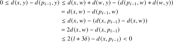 $$ \begin{align*} 0 \leq d(x,y)-d(p_{i-1},y) & \leq d(x,w)+d(w,y) - (d(p_{i-1},w)+d(w,y))\\ & = d(x,w)-d(p_{i-1},w)\\ & \leq d(x,w)-(d(x,p_{i-1})-d(x,w))\\ & = 2d(x,w)-d(x,p_{i-1})\\ & \leq 2(l+3\delta) - d(x,p_{i-1}) < 0 \end{align*} $$
a contradiction. We have thus established that $M \le l+ 3\delta $
, and so c lies in the
$M \le l+ 3\delta $
, and so c lies in the $l+3\delta $
–neighborhood of
$l+3\delta $
–neighborhood of $\gamma $
.
$\gamma $
.
Definition 2.11. Let $r>0$
, and let M be a metric space. A subset S of M is r–connected if any two points
$r>0$
, and let M be a metric space. A subset S of M is r–connected if any two points $p,q$
of S can be connected by a chain of points in S,
$p,q$
of S can be connected by a chain of points in S,
 $$\begin{align*}p = p_0,\ p_1,\ldots, p_k = q,\end{align*}$$
so that $d_M(p_i,p_{i+1})\leq r$
for all i. An r–connected component of S is a maximal subset of S which is r–connected.
$d_M(p_i,p_{i+1})\leq r$
for all i. An r–connected component of S is a maximal subset of S which is r–connected.
Lemma 2.12. Let $H> 0$
, and let
$H> 0$
, and let $R> 24 H + 16 \delta $
. Let
$R> 24 H + 16 \delta $
. Let $S\subset \Gamma $
be a
$S\subset \Gamma $
be a $\frac {R}{4}$
-connected set so that for every
$\frac {R}{4}$
-connected set so that for every $s\in S$
, there is a biinfinite geodesic
$s\in S$
, there is a biinfinite geodesic $\gamma _s$
satisfying:
$\gamma _s$
satisfying:
 $$\begin{align*}S\cap B_R(s)\subset N_H(\gamma_s),\mbox{ and } \gamma_s\cap B_R(s)\subset N_H(S).\end{align*}$$
Then there is an oriented biinfinite geodesic $\gamma $
so that
$\gamma $
so that
-
1.
$d_{\mathrm {Haus}}(\gamma ,S)\le 3 H + 6\delta $
; and -
2. for every
$s\in S$
, we may orient
$\gamma _s$
so the Gromov products
$({\gamma ^{+\infty }}\,|\,{\gamma _s^{+\infty }})_{s}$
and
$({\gamma ^{-\infty }}\,|\,{\gamma _s^{-\infty }})_{s}$
are bounded below by
$R - (4H+10\delta )$
.


Proof. Choose any $s_0$
in S, and let
$s_0$
in S, and let $\gamma _0 = \gamma _{s_0}$
be a biinfinite geodesic as in the hypothesis, parameterized so that
$\gamma _0 = \gamma _{s_0}$
be a biinfinite geodesic as in the hypothesis, parameterized so that $\gamma _0(0)$
is within H of
$\gamma _0(0)$
is within H of $s_0$
. Since the points
$s_0$
. Since the points $\gamma _0(\pm \frac {R}{2})$
lie in
$\gamma _0(\pm \frac {R}{2})$
lie in $B_R(s)$
, there are points
$B_R(s)$
, there are points $s_{\pm 1}\in S$
whose distances from
$s_{\pm 1}\in S$
whose distances from $\gamma _0(\pm \frac {R}{2})$
are at most H. Since
$\gamma _0(\pm \frac {R}{2})$
are at most H. Since $d_{\Gamma }(s_0,s_{\pm 1})\le \frac {R}{2} + 2 H$
and
$d_{\Gamma }(s_0,s_{\pm 1})\le \frac {R}{2} + 2 H$
and $d_{\Gamma }(s_{-1},s_1)\ge R- 2 H$
, we deduce
$d_{\Gamma }(s_{-1},s_1)\ge R- 2 H$
, we deduce $({s_{-1}}\,|\,{s_1})_{s_0}\leq 3 H$
. In particular, we have the following estimates:
$({s_{-1}}\,|\,{s_1})_{s_0}\leq 3 H$
. In particular, we have the following estimates:
 $$ \begin{align} d_{\Gamma}(s_0,s_{\pm 1}) \ge \frac{R}{2}-2H\mbox{ and }({s_{-1}}\,|\,{s_1})_{s_0}\leq 3 H. \end{align} $$
Now, we inductively find $s_i$
and
$s_i$
and $\gamma _i$
for all integers i.
$\gamma _i$
for all integers i.
For clarity, we focus on $i>1$
. The construction for
$i>1$
. The construction for $i<0$
is entirely analogous. Suppose we have chosen points
$i<0$
is entirely analogous. Suppose we have chosen points $s_{-1},s_0,\ldots s_{i-1}$
in S, and that for each positive
$s_{-1},s_0,\ldots s_{i-1}$
in S, and that for each positive $j\le i-1$
, we have chosen a biinfinite geodesic
$j\le i-1$
, we have chosen a biinfinite geodesic $\gamma _j = \gamma _{s_j}$
, and some
$\gamma _j = \gamma _{s_j}$
, and some $t_j$
within
$t_j$
within $4H$
of
$4H$
of $-\frac {R}{2}$
so that
$-\frac {R}{2}$
so that
 $$ \begin{align*} d_{\Gamma}(\gamma_{i-1}(0),s_{i-1})& \le H,\mbox{ and }\\ d_{\Gamma}(\gamma_{i-1}(t_{i-1}),s_{i-2})& \le H. \end{align*} $$
Since $R>8H$
, the number
$R>8H$
, the number $t_{i-1}$
is negative. The point
$t_{i-1}$
is negative. The point $\gamma _{i-1}(\frac {R}{2})$
lies in the R–ball around
$\gamma _{i-1}(\frac {R}{2})$
lies in the R–ball around $s_{i-1}$
, so we may choose a point
$s_{i-1}$
, so we may choose a point $s_i\in S$
so that
$s_i\in S$
so that $d_{\Gamma }(s_i,\gamma _{i-1}(\frac {R}{2}))\le H$
. Let
$d_{\Gamma }(s_i,\gamma _{i-1}(\frac {R}{2}))\le H$
. Let $\gamma _i$
be the geodesic
$\gamma _i$
be the geodesic $\gamma _{s_i}$
provided by the hypothesis of the lemma. We can assume that
$\gamma _{s_i}$
provided by the hypothesis of the lemma. We can assume that $\gamma _i(0)$
is within H of
$\gamma _i(0)$
is within H of $s_i$
. The distance
$s_i$
. The distance $d_{\Gamma }(s_{i-1},s_i)$
differs from
$d_{\Gamma }(s_{i-1},s_i)$
differs from $\frac {R}{2}$
by at most
$\frac {R}{2}$
by at most $2H$
. Thus, for some
$2H$
. Thus, for some $t_i$
of absolute value in
$t_i$
of absolute value in $[\frac {R}{2}-4H,\frac {R}{2}+4H]$
, we have
$[\frac {R}{2}-4H,\frac {R}{2}+4H]$
, we have $d_{\Gamma }(\gamma _i(t_i),s_{i-1})\le H$
. We parameterize
$d_{\Gamma }(\gamma _i(t_i),s_{i-1})\le H$
. We parameterize $\gamma _i$
so that
$\gamma _i$
so that $t_i<0$
. This completes the inductive construction.
$t_i<0$
. This completes the inductive construction.
From the construction, we have
 $$ \begin{align} d_{\Gamma}(s_i,s_{i+1})\le \frac{R}{2} + 2 H \end{align} $$
and
 $$ \begin{align*} d_{\Gamma}(s_{i-1},s_{i+1}) \ge \frac{R}{2}+ |t_i| - 2 H \ge R - 6 H \end{align*} $$
(the lower bound when $i=0$
is slightly better). This implies a bound on Gromov products
$i=0$
is slightly better). This implies a bound on Gromov products
 $$ \begin{align} ({s_{i-1}}\,|\,{s_{i+1}})_{s_i} \le 5 H. \end{align} $$
Let $c_k$
be a piecewise geodesic formed by concatenating geodesics
$c_k$
be a piecewise geodesic formed by concatenating geodesics
 $$\begin{align*}[s_{-k},s_{-k+1}]\cdots [s_{k-1},s_k]. \end{align*}$$
We verify the hypotheses of Lemma 2.10 with $l = 5H$
. The inequality (6) gives the bound on Gromov products in the corners. The inequality (5) gives that the segments
$l = 5H$
. The inequality (6) gives the bound on Gromov products in the corners. The inequality (5) gives that the segments $[s_i,s_{i+1}]$
have length at least
$[s_i,s_{i+1}]$
have length at least $\frac {R}{2} - 2H> 10 H + 8 \delta = 2 l + 8\delta $
as required. Thus, if
$\frac {R}{2} - 2H> 10 H + 8 \delta = 2 l + 8\delta $
as required. Thus, if $\beta _k$
is the geodesic joining the endpoints of
$\beta _k$
is the geodesic joining the endpoints of $c_k$
, we have
$c_k$
, we have $d_{\mathrm {Haus}}(c_k,\beta _k)\le H + 4\delta $
.
$d_{\mathrm {Haus}}(c_k,\beta _k)\le H + 4\delta $
.
Since $\Gamma $
is proper, and the geodesics
$\Gamma $
is proper, and the geodesics $\beta _k$
all pass through the
$\beta _k$
all pass through the $(H+4\delta )$
–ball about
$(H+4\delta )$
–ball about $s_0$
, they subconverge to a biinfinite geodesic
$s_0$
, they subconverge to a biinfinite geodesic $\gamma $
. Notice that all the segments
$\gamma $
. Notice that all the segments $[s_i,s_{i+1}]$
lie in the
$[s_i,s_{i+1}]$
lie in the $(H+4\delta )$
–neighborhood of
$(H+4\delta )$
–neighborhood of $\gamma $
. We will show this
$\gamma $
. We will show this $\gamma $
satisfies the conclusions of the lemma.
$\gamma $
satisfies the conclusions of the lemma.
If $s\in S$
, then there is a
$s\in S$
, then there is a $\frac {R}{4}$
–coarse path joining
$\frac {R}{4}$
–coarse path joining $s_0$
to s, that is to say there exist points
$s_0$
to s, that is to say there exist points $s_0=p_0 ,\ p_1,\ \ldots ,\ p_k = s$
in S satisfying.
$s_0=p_0 ,\ p_1,\ \ldots ,\ p_k = s$
in S satisfying.
 $$\begin{align*}d_{\Gamma}(p_i,p_{i+1})\le \frac{R}{4},\ \forall i. \end{align*}$$
We first claim that for each $p_i$
, there is some
$p_i$
, there is some $s_{j(i)}$
with
$s_{j(i)}$
with $d_{\Gamma }(s_{j(i)},p_i)\le \frac {R}{4}+2 H$
. Clearly this is true for
$d_{\Gamma }(s_{j(i)},p_i)\le \frac {R}{4}+2 H$
. Clearly this is true for $p_0$
. Arguing by induction, we see that
$p_0$
. Arguing by induction, we see that $d_{\Gamma }(p_{i+1},s_{j(i)})$
is at most
$d_{\Gamma }(p_{i+1},s_{j(i)})$
is at most $\frac {R}{2}+2 H$
. In particular, there is a point q on
$\frac {R}{2}+2 H$
. In particular, there is a point q on $\gamma _{s_{j(i)}}$
within H of
$\gamma _{s_{j(i)}}$
within H of $p_{i+1}$
. Recalling that
$p_{i+1}$
. Recalling that $\gamma _{s_{j(i)}}(0)$
lies within H of
$\gamma _{s_{j(i)}}(0)$
lies within H of $s_{j(i)}$
, we see that
$s_{j(i)}$
, we see that $q = \gamma _{s_{j(i)}}(t)$
for some t with
$q = \gamma _{s_{j(i)}}(t)$
for some t with
 $$\begin{align*}|t| \le \frac{R}{2} + 3H<\frac{3}{4}R.\end{align*}$$
Thus, for some $t' \in \{-\frac {R}{2}, 0, \frac {R}{2}\}$
, we have
$t' \in \{-\frac {R}{2}, 0, \frac {R}{2}\}$
, we have $|t-t'|\le \frac {R}{4}$
. Since the points
$|t-t'|\le \frac {R}{4}$
. Since the points $\gamma _{s_{j(i)}}(\pm \frac {R}{2})$
are within H of
$\gamma _{s_{j(i)}}(\pm \frac {R}{2})$
are within H of $s_{j(i)\pm 1}$
, there is some
$s_{j(i)\pm 1}$
, there is some $s_{j(i+1)}\in \{s_{j(i)-1},s_{j(i)},s_{j(i)+1}\}$
so that
$s_{j(i+1)}\in \{s_{j(i)-1},s_{j(i)},s_{j(i)+1}\}$
so that $d_{\Gamma }(p_{i+1},s_{j(i+1)}) \le 2H + \frac {R}{4}$
, as desired.
$d_{\Gamma }(p_{i+1},s_{j(i+1)}) \le 2H + \frac {R}{4}$
, as desired.
Now let $s_j = s_{j(k)}$
, so we have
$s_j = s_{j(k)}$
, so we have $d_{\Gamma }(s,s_j)\le \frac {R}{4} + 2H$
, and let q be a closest point to s on
$d_{\Gamma }(s,s_j)\le \frac {R}{4} + 2H$
, and let q be a closest point to s on $\gamma _j$
. Without loss of generality, we suppose that
$\gamma _j$
. Without loss of generality, we suppose that $q = \gamma _j(t)$
for
$q = \gamma _j(t)$
for $t\ge 0$
. Any quadrilateral with corners
$t\ge 0$
. Any quadrilateral with corners $s_j, s_{j+1},\gamma _j(0),\gamma _j(\frac {R}{2})$
is
$s_j, s_{j+1},\gamma _j(0),\gamma _j(\frac {R}{2})$
is $2\delta $
–thin, so there is a point r on
$2\delta $
–thin, so there is a point r on $[s_j,s_{j+1}]$
within
$[s_j,s_{j+1}]$
within $H+2\delta $
of q. This point r is within
$H+2\delta $
of q. This point r is within $H+4\delta $
of some point z on
$H+4\delta $
of some point z on $\gamma $
. Adding up the constants, we have
$\gamma $
. Adding up the constants, we have
 $$ \begin{align*} d_{\Gamma}(s,z) & \le d_{\Gamma}(s,q) + d_{\Gamma}(q,r) + d_{\Gamma}(r,z)\\ & \le H + H + 2\delta + H + 4\delta = 3H + 6\delta. \end{align*} $$
This shows
 $$ \begin{align} S \subset N_{3H + 6\delta}(\gamma). \end{align} $$
Conversely, let $x\in \gamma $
. Then
$x\in \gamma $
. Then $x\in \beta _k$
for some k, and so for some i, there is a point
$x\in \beta _k$
for some k, and so for some i, there is a point $y\in [s_i,s_{i+1}]$
with
$y\in [s_i,s_{i+1}]$
with $d_{\Gamma }(x,y)\le H + 4\delta $
. This point is within
$d_{\Gamma }(x,y)\le H + 4\delta $
. This point is within $H+2\delta $
of a point on
$H+2\delta $
of a point on $\gamma _i$
, which is within H of a point of S, so we have
$\gamma _i$
, which is within H of a point of S, so we have
 $$ \begin{align} \gamma \subset N_{3H+6\delta} (S). \end{align} $$
Together, (7) and (8) imply the first statement of the lemma, that is to say the bound on Hausdorff distance. It remains to show the statement about Gromov products. Breaking symmetry, we consider just the ray $\gamma _s|[0,\infty )$
. Let
$\gamma _s|[0,\infty )$
. Let $y'$
be a point on
$y'$
be a point on $\gamma _s|[0,\infty )$
at distance R from s. Let
$\gamma _s|[0,\infty )$
at distance R from s. Let $s'\in S$
be a point within H of
$s'\in S$
be a point within H of $y'$
, and let
$y'$
, and let $z'$
be a point on
$z'$
be a point on $\gamma $
within
$\gamma $
within $3H + 6\delta $
of
$3H + 6\delta $
of $s'$
. Let
$s'$
. Let $\alpha $
be a ray starting at s with limit point
$\alpha $
be a ray starting at s with limit point $\gamma _s^{+\infty }$
, and let
$\gamma _s^{+\infty }$
, and let $\beta $
be a ray starting at s with limit point
$\beta $
be a ray starting at s with limit point $\gamma ^{+\infty }$
. There are points y on
$\gamma ^{+\infty }$
. There are points y on $\alpha $
and z on
$\alpha $
and z on $\beta $
which are within
$\beta $
which are within $\delta $
of
$\delta $
of $y'$
,
$y'$
, $z'$
, respectively. We have
$z'$
, respectively. We have $d_{\Gamma }(s,y)\ge R-\delta $
,
$d_{\Gamma }(s,y)\ge R-\delta $
, $d_{\Gamma }(s,z) \ge R - (4H + 7\delta )$
and
$d_{\Gamma }(s,z) \ge R - (4H + 7\delta )$
and $d_{\Gamma }(y,z) \le 3H + 8\delta $
, so
$d_{\Gamma }(y,z) \le 3H + 8\delta $
, so
 $$\begin{align*}({y}\,|\,{z})_{s} \ge \frac{1}{2}(R - \delta + R-(4H + 7\delta) - (4 H + 8\delta)) = R-(4H + 8\delta). \end{align*}$$
Lemma 2.1 allows us to conclude $({\gamma _s^{+\infty }}\,|\,{\gamma ^{+\infty }})_{s} \ge R - (4H + 10\delta )$
, as desired.
$({\gamma _s^{+\infty }}\,|\,{\gamma ^{+\infty }})_{s} \ge R - (4H + 10\delta )$
, as desired.
3 An equivariant map from
$X\times \partial G$
to itself

The first step in the proof of Theorem 1.1 is the following construction, which can be thought of as a generalization of that in [Reference Bowden and MannBM19, Lemma 3.1]. If X is a space with a proper, free, and cocompact action of G, and $\rho \colon \thinspace G \to \mathrm {Homeo}(Y)$
an action of G on a topological space, one can capture the information of this action as the holonomy of a foliated Y-bundle over
$\rho \colon \thinspace G \to \mathrm {Homeo}(Y)$
an action of G on a topological space, one can capture the information of this action as the holonomy of a foliated Y-bundle over $X/G$
; this is simply the quotient of
$X/G$
; this is simply the quotient of $X \times Y$
by the diagonal action of G. Here, the case of interest to us is when
$X \times Y$
by the diagonal action of G. Here, the case of interest to us is when $Y = \partial G = S^n$
. The following proposition gives a construction of a “nice” map between the foliated bundles associated to the boundary action
$Y = \partial G = S^n$
. The following proposition gives a construction of a “nice” map between the foliated bundles associated to the boundary action $\rho _0$
and a small perturbation
$\rho _0$
and a small perturbation $\rho $
.
$\rho $
.
The same proof works with any manifold Y in place of $S^n$
, and any two nearby actions of an arbitrary group G on the space, so we state it in this general context, as follows.
$S^n$
, and any two nearby actions of an arbitrary group G on the space, so we state it in this general context, as follows.
Let Y be a metric space, such that $\mathrm {Homeo}(Y)$
is metrizable and locally contractible. For instance, one may take Y to be any compact manifold, in which case local contractibility of
$\mathrm {Homeo}(Y)$
is metrizable and locally contractible. For instance, one may take Y to be any compact manifold, in which case local contractibility of $\mathrm {Homeo}(Y)$
follows from Edwards–Kirby [Reference Edwards and KirbyEK71]. Metrizability of
$\mathrm {Homeo}(Y)$
follows from Edwards–Kirby [Reference Edwards and KirbyEK71]. Metrizability of $\mathrm {Homeo}(Y)$
has the following easy consequence.
$\mathrm {Homeo}(Y)$
has the following easy consequence.
Observation 3.1.
Let W be a neighborhood of the identity in $\mathrm {Homeo}(Y)$
, and let
$\mathrm {Homeo}(Y)$
, and let $F\subset \mathrm {Homeo}(Y)$
be finite. Then there is a neighborhood
$F\subset \mathrm {Homeo}(Y)$
be finite. Then there is a neighborhood $V \subset W$
of the identity so that the union
$V \subset W$
of the identity so that the union
 $$\begin{align*}\bigcup_{f\in F} f V f^{-1} V \end{align*}$$
lies in W.
Using this, we prove the following.
Proposition 3.2. Let G be a group, Y a metric space as above, and fix an action $\rho _0\colon \thinspace G \to \mathrm {Homeo}(Y)$
. Let X be a metric space on which G acts properly, freely, and cocompactly by isometries.
$\rho _0\colon \thinspace G \to \mathrm {Homeo}(Y)$
. Let X be a metric space on which G acts properly, freely, and cocompactly by isometries.
For any compact $K \subset X$
and
$K \subset X$
and $\epsilon>0$
, there is a neighborhood U of
$\epsilon>0$
, there is a neighborhood U of $\rho _0$
, so that for each
$\rho _0$
, so that for each $\rho \in U$
, there is a homeomorphism
$\rho \in U$
, there is a homeomorphism $f^\rho \colon \thinspace X\times Y \to X\times Y$
with the following properties:
$f^\rho \colon \thinspace X\times Y \to X\times Y$
with the following properties:
-
1. (Covers
$\mathrm {id}_X$
) If
$\pi _X$
is the projection from
$X\times Y$
to X, then
$\pi _X\circ f^\rho = \pi _X$
. In other words,
$f^\rho $
covers the identity on X. -
2. (Equivariance) For every
$g \in G$
, we have
$$\begin{align*}f^\rho(g\cdot x,\rho(g)\cdot\theta) = (g,\rho_0(g))\cdot f^\rho(x,\theta) .\end{align*}$$
-
3. (Near flatness.) For any
$\theta \in Y$
, we have
$$\begin{align*}f^\rho(K\times\{\theta\}) \subset X \times B_\epsilon(\theta). \end{align*}$$


Proof of Proposition 3.2
Since the action is proper, free, and cocompact, there is some $r>0$
so that every nontrivial element of G moves every point of X a distance at least r. Choose a G–equivariant locally finite cover
$r>0$
so that every nontrivial element of G moves every point of X a distance at least r. Choose a G–equivariant locally finite cover $\mathcal {U}=\{U_i\mid i\in I\}$
of X by open balls of radius
$\mathcal {U}=\{U_i\mid i\in I\}$
of X by open balls of radius $r/3$
, and let N be the nerve of
$r/3$
, and let N be the nerve of $\mathcal {U}$
. Since
$\mathcal {U}$
. Since $\mathcal {U}$
was G–equivariant and locally finite, the group G acts cocompactly on the simplicial complex N. Since any
$\mathcal {U}$
was G–equivariant and locally finite, the group G acts cocompactly on the simplicial complex N. Since any $g\in G-\{1\}$
moves every set
$g\in G-\{1\}$
moves every set $U_i$
off of itself, G acts freely on N.
$U_i$
off of itself, G acts freely on N.
We choose a G–equivariant partition of unity $\{\phi _i\colon \thinspace X\to [0,1]\mid i\in I\}$
subordinate to the cover
$\{\phi _i\colon \thinspace X\to [0,1]\mid i\in I\}$
subordinate to the cover $\mathcal {U}$
. This partition determines a proper G–equivariant map
$\mathcal {U}$
. This partition determines a proper G–equivariant map $\psi \colon \thinspace X\to N$
.
$\psi \colon \thinspace X\to N$
.
To define $f^\rho $
, we first define a map
$f^\rho $
, we first define a map $ \varphi ^\rho \colon \thinspace N\to \mathrm {Homeo}(Y)$
, and then define
$ \varphi ^\rho \colon \thinspace N\to \mathrm {Homeo}(Y)$
, and then define
 $$ \begin{align} f^\rho( x, \theta ) = \left(x, (\varphi^\rho \circ \psi (x) )(\theta)\right). \end{align} $$
The map $\varphi ^\rho $
will be G–equivariant with respect to the “mixed” left action of G by homeomorphisms of
$\varphi ^\rho $
will be G–equivariant with respect to the “mixed” left action of G by homeomorphisms of $\mathrm {Homeo}(Y)$
given by
$\mathrm {Homeo}(Y)$
given by
 $$ \begin{align} g \cdot h = \rho_0(g) h \rho(g^{-1}). \end{align} $$
Definition of $ {\varphi }^{\rho }$
.
$ {\varphi }^{\rho }$
.
The definition of $\varphi ^\rho $
is designed to keep track of the compact set K and constant
$\varphi ^\rho $
is designed to keep track of the compact set K and constant $\epsilon>0$
for the near flatness condition in the proposition. Let D be a connected union of open simplices in N which meets every G–orbit exactly once. Let K be a compact subcomplex of N, which we assume contains the closed star of any cell of
$\epsilon>0$
for the near flatness condition in the proposition. Let D be a connected union of open simplices in N which meets every G–orbit exactly once. Let K be a compact subcomplex of N, which we assume contains the closed star of any cell of $\overline {D}$
(note that any compact
$\overline {D}$
(note that any compact $C\subset X$
has
$C\subset X$
has $\psi (C)\subset K$
for some such complex). Let
$\psi (C)\subset K$
for some such complex). Let $\epsilon>0$
. Let S be the (finite) set of group elements s so that
$\epsilon>0$
. Let S be the (finite) set of group elements s so that $sD$
meets the closed star of some vertex in
$sD$
meets the closed star of some vertex in $\overline {D}$
. Let F be the (still finite) set of group elements g, so that
$\overline {D}$
. Let F be the (still finite) set of group elements g, so that $gD\cap K$
is nonempty.
$gD\cap K$
is nonempty.
Letting $W = N_\epsilon (\mathrm {id})$
, we choose a neighborhood V as in Observation 3.1 so that
$W = N_\epsilon (\mathrm {id})$
, we choose a neighborhood V as in Observation 3.1 so that $\rho _0(g)V\rho _0(g)^{-1}V$
lies in W for all
$\rho _0(g)V\rho _0(g)^{-1}V$
lies in W for all $g\in F$
. Now let
$g\in F$
. Now let $m = \dim (N)$
. Apply Observation 3.1 and local contractibility of
$m = \dim (N)$
. Apply Observation 3.1 and local contractibility of $\mathrm {Homeo}(Y)$
to choose a nested sequence of contractible neighborhoods of
$\mathrm {Homeo}(Y)$
to choose a nested sequence of contractible neighborhoods of $1$
inside V:
$1$
inside V:
 $$\begin{align*}V_0\subset V_1 \subset \cdots \subset V_m \subset V \end{align*}$$
so that for each i and all $s\in S$
, we have
$s\in S$
, we have
 $$ \begin{align} \rho_0(s) V_i \rho_0(s)^{-1} V_i \subset V_{i+1}. \end{align} $$
By taking $\rho $
sufficiently close to
$\rho $
sufficiently close to $\rho _0$
, we may assume that
$\rho _0$
, we may assume that $\rho _0(g)\rho (g^{-1})$
lies in
$\rho _0(g)\rho (g^{-1})$
lies in $V_0$
for all
$V_0$
for all $g\in F$
. We define
$g\in F$
. We define $\varphi ^\rho $
inductively over the k–skeleta of N in such a way that
$\varphi ^\rho $
inductively over the k–skeleta of N in such a way that $\varphi ^\rho (\sigma ) \subset V_k$
for every k–cell in the closed star of a vertex of
$\varphi ^\rho (\sigma ) \subset V_k$
for every k–cell in the closed star of a vertex of $\overline {D}$
.
$\overline {D}$
.
0-skeleton. Define $\varphi ^\rho $
on
$\varphi ^\rho $
on $N^{(0)}$
as follows. If
$N^{(0)}$
as follows. If $v = g v_0$
for some
$v = g v_0$
for some $v_0\in D$
, then
$v_0\in D$
, then
 $$\begin{align*}\varphi^\rho(v) = \rho_0(g)\rho(g^{-1}) .\end{align*}$$
If v lies in the closed star of some cell of D, then $g\in S$
, so
$g\in S$
, so $\varphi ^\rho (v)\in V_0$
as desired.
$\varphi ^\rho (v)\in V_0$
as desired.
Inductive step. Suppose that $\varphi ^\rho $
has been defined on all
$\varphi ^\rho $
has been defined on all $(k-1)$
–cells, and let
$(k-1)$
–cells, and let $\sigma $
be a k–cell. We may write
$\sigma $
be a k–cell. We may write $\sigma = g\sigma _0$
, where
$\sigma = g\sigma _0$
, where $\sigma _0$
is an open k–cell in D. The map
$\sigma _0$
is an open k–cell in D. The map $\varphi ^\rho $
has already been defined on the boundary of
$\varphi ^\rho $
has already been defined on the boundary of $\sigma _0$
, and sends this boundary into
$\sigma _0$
, and sends this boundary into $V_{k-1}$
by induction. Using the contractibility of
$V_{k-1}$
by induction. Using the contractibility of $V_{k-1}$
, we extend
$V_{k-1}$
, we extend $\varphi ^\rho $
over
$\varphi ^\rho $
over $\sigma _0$
in such a way that
$\sigma _0$
in such a way that $\varphi ^\rho (\sigma _0)\subset V_{k-1}$
. We define
$\varphi ^\rho (\sigma _0)\subset V_{k-1}$
. We define $\varphi ^\rho |_{\sigma (x)} = \rho _0(g)\varphi ^\rho (g^{-1}(x))\rho (g^{-1})$
. Since the action on N is free, there is no ambiguity in this definition.
$\varphi ^\rho |_{\sigma (x)} = \rho _0(g)\varphi ^\rho (g^{-1}(x))\rho (g^{-1})$
. Since the action on N is free, there is no ambiguity in this definition.
Now suppose that $\sigma $
lies in the closed star of some vertex of
$\sigma $
lies in the closed star of some vertex of $\overline {D}$
, so
$\overline {D}$
, so $\sigma = s\sigma _0$
for some
$\sigma = s\sigma _0$
for some $s\in S$
. The set
$s\in S$
. The set $\varphi ^\rho (\sigma )$
lies in
$\varphi ^\rho (\sigma )$
lies in
 $$\begin{align*}\rho_0(s) V_{k-1} \rho(s^{-1}) = \rho_0(s) V_{k-1} \rho_0(s)^{-1}\rho_0(s) \rho(s)^{-1}\subset \rho_0(s) V_{k-1} \rho_0(s)^{-1}V_0,\end{align*}$$
which lies in $V_k$
by (11). Having verified the inductive hypothesis, we see that we can continue until we have defined
$V_k$
by (11). Having verified the inductive hypothesis, we see that we can continue until we have defined $\varphi ^\rho $
equivariantly on all of N. Moreover, we have defined it so that
$\varphi ^\rho $
equivariantly on all of N. Moreover, we have defined it so that $\varphi ^\rho (\sigma _0)$
lies in the neighborhood V for any
$\varphi ^\rho (\sigma _0)$
lies in the neighborhood V for any $\sigma _0$
meeting D.
$\sigma _0$
meeting D.
Properties of ${f}^{\rho }$
Having defined $\varphi ^\rho $
, we define
$\varphi ^\rho $
, we define $f^{\rho }$
as in (9).
$f^{\rho }$
as in (9).
 $$ \begin{align*} f^\rho( x, \theta ) = \left(x, (\varphi^\rho \circ \psi (x) )(\theta)\right). \end{align*} $$
By definition, this covers the identity map on X. To simplify notation, let $\Phi ^\rho $
denote
$\Phi ^\rho $
denote $\varphi ^\rho \circ \psi $
. Note that
$\varphi ^\rho \circ \psi $
. Note that $\Phi ^\rho $
satisfies equivariance as
$\Phi ^\rho $
satisfies equivariance as $\varphi ^\rho $
does. This also gives equivariance of
$\varphi ^\rho $
does. This also gives equivariance of $f^\rho $
, as follows:
$f^\rho $
, as follows:
 $$ \begin{align*} f^\rho(g\cdot x,\rho(g)\cdot\theta) & = \left( g\cdot x, \left(\Phi^\rho(g\cdot x)\rho(g)\right)\cdot \theta\right) \\ & = \left( g\cdot x, \left(\rho_0(g)\Phi^\rho(x)\rho(g^{-1})\rho(g)\right)\cdot \theta\right) \\ & = \left( g\cdot x, \left(\rho_0(g)\Phi^\rho(x)\right)\cdot \theta\right) \\ & = \left( g,\rho_0(g)\right)\cdot \left(x,\Phi^\rho(x)\cdot \theta\right) \\ & = \left( g,\rho_0(g)\right)\cdot f^\rho( x, \theta ). \end{align*} $$
It remains to check near flatness. For any cell $\sigma $
of the larger compact complex K, there is some
$\sigma $
of the larger compact complex K, there is some $g\in F$
and some
$g\in F$
and some $\sigma _0\subset D$
so that
$\sigma _0\subset D$
so that $\sigma = g \sigma _0$
. Equivariance tells us that
$\sigma = g \sigma _0$
. Equivariance tells us that
 $$ \begin{align*} \varphi^\rho(\sigma) & = \rho_0(g)\varphi^\rho(\sigma_0)\rho(g^{-1})\\ & = \rho_0(g)\varphi^\rho(\sigma_0)\rho_0(g)^{-1} \cdot \rho_0(g)\rho(g^{-1}) \\ & \subset \rho_0(g) V \rho_0(g)^{-1} \cdot V \subset W. \end{align*} $$
Since every homeomorphism in W moves every point of Y a distance of at most $\epsilon $
, we have
$\epsilon $
, we have $f^\rho (\sigma \times \{\theta \})\subset B_\epsilon (\theta )$
as desired.
$f^\rho (\sigma \times \{\theta \})\subset B_\epsilon (\theta )$
as desired.
4 Reduction to the main case
In this section, we reduce to the case $\partial G = S^n$
for
$\partial G = S^n$
for $n \geq 2$
, and also to the case where G acts faithfully on its boundary. The first reduction (to
$n \geq 2$
, and also to the case where G acts faithfully on its boundary. The first reduction (to $n\ge 2$
) comes from combining work of Matsumoto with the Convergence Group Theorem.
$n\ge 2$
) comes from combining work of Matsumoto with the Convergence Group Theorem.
Proposition 4.1. Let G be a hyperbolic group with circle boundary. Then the action of G on $\partial G$
is topologically stable.
$\partial G$
is topologically stable.
This can quite likely be derived from Matsumoto’s original proof, as the main techniques are Euler characteristic and lifting to covers. For completeness, we give a short argument using standard tools from circle dynamics.
Proof. Let G be a hyperbolic group with circle boundary. By the Convergence Group Theorem [Reference GabaiGab92, Reference Casson and JungreisCJ94], there exists a normal, finite index torsion-free subgroup $G'$
of G that is isomorphic to the fundamental group of a closed surface. Let
$G'$
of G that is isomorphic to the fundamental group of a closed surface. Let $\rho $
be a perturbation of the standard boundary action
$\rho $
be a perturbation of the standard boundary action $\rho _0$
of G. By [Reference MatsumotoMat87], there exists a continuous, surjective, degree one map
$\rho _0$
of G. By [Reference MatsumotoMat87], there exists a continuous, surjective, degree one map $h: S^1 \to S^1$
, such that
$h: S^1 \to S^1$
, such that $h \rho (g) = \rho _0(g) h$
for each
$h \rho (g) = \rho _0(g) h$
for each $g \in G'$
. If the action of
$g \in G'$
. If the action of $G'$
is minimal, then h is a conjugacy. If the action of
$G'$
is minimal, then h is a conjugacy. If the action of $G'$
is not minimal, then there exists a unique invariant exceptional minimal set X, homeomorphic to a Cantor set, and h collapses the closure of each complementary interval to a point and is otherwise injective (see e.g. [Reference GhysGhy01, Proposition 5.6]). It is also easy to see that h varies continuously with
$G'$
is not minimal, then there exists a unique invariant exceptional minimal set X, homeomorphic to a Cantor set, and h collapses the closure of each complementary interval to a point and is otherwise injective (see e.g. [Reference GhysGhy01, Proposition 5.6]). It is also easy to see that h varies continuously with $\rho $
, so can be taken as close to the identity as desired by taking
$\rho $
, so can be taken as close to the identity as desired by taking $\rho $
close to
$\rho $
close to $\rho _0$
.
$\rho _0$
.
Since $G'$
is normal in G, the set X is
$G'$
is normal in G, the set X is $\rho (G)$
-invariant. It follows that G permutes the point-preimages of h. From this, we will now deduce that h in fact defines a semiconjugacy intertwining the actions of
$\rho (G)$
-invariant. It follows that G permutes the point-preimages of h. From this, we will now deduce that h in fact defines a semiconjugacy intertwining the actions of $\rho _0(G)$
and
$\rho _0(G)$
and $\rho (G)$
. To see this, we use the fact that attracting fixed points of elements of
$\rho (G)$
. To see this, we use the fact that attracting fixed points of elements of $\rho _0(G')$
are dense in
$\rho _0(G')$
are dense in $S^1$
. If x is the attracting fixed point of
$S^1$
. If x is the attracting fixed point of $\rho _0(\gamma )$
for some
$\rho _0(\gamma )$
for some $\gamma \in G'$
, then
$\gamma \in G'$
, then $\rho _0(g)x$
is the attracting fixed point of
$\rho _0(g)x$
is the attracting fixed point of $\rho _0(g\gamma g^{-1})$
, an element which also lies in
$\rho _0(g\gamma g^{-1})$
, an element which also lies in $G'$
. Thus, for any
$G'$
. Thus, for any $y \in h^{-1}(x)$
, we have
$y \in h^{-1}(x)$
, we have $\rho (g)(y) \in h^{-1}\rho _0(g)(x)$
; equivalently,
$\rho (g)(y) \in h^{-1}\rho _0(g)(x)$
; equivalently, $h \rho (g)(y) = \rho _0(g) h(y)$
. Since h is continuous, and the union of preimages of attracting fixed points is dense in
$h \rho (g)(y) = \rho _0(g) h(y)$
. Since h is continuous, and the union of preimages of attracting fixed points is dense in $S^1$
, this shows that
$S^1$
, this shows that $h \rho (g) = \rho _0(g) h$
holds globally.
$h \rho (g) = \rho _0(g) h$
holds globally.
Proposition 4.2. Suppose G is a hyperbolic group with sphere boundary, and let $F<G$
be the subgroup of elements which act trivially on
$F<G$
be the subgroup of elements which act trivially on $\partial G$
. Then G is topologically stable if and only if
$\partial G$
. Then G is topologically stable if and only if $G/F$
is topologically stable.
$G/F$
is topologically stable.
Proof. Since F is a finite normal subgroup, the canonical action of G on its boundary factors through the canonical action of $G/F$
on its boundary, and these boundaries are the same. Let N be the maximum order of an element of F. By a theorem of Newman [Reference NewmanNew31], there is a neighborhood U of the identity in
$G/F$
on its boundary, and these boundaries are the same. Let N be the maximum order of an element of F. By a theorem of Newman [Reference NewmanNew31], there is a neighborhood U of the identity in $\mathrm {Homeo}(S^n)$
so that any torsion element in U has order greater than N. Thus, for any sufficiently small perturbation of the canonical action, the elements of F will still act trivially, and so small perturbations of the canonical action of G on its boundary are in one-to-one correspondence with small perturbations of
$\mathrm {Homeo}(S^n)$
so that any torsion element in U has order greater than N. Thus, for any sufficiently small perturbation of the canonical action, the elements of F will still act trivially, and so small perturbations of the canonical action of G on its boundary are in one-to-one correspondence with small perturbations of $G/F$
on its boundary.
$G/F$
on its boundary.
We therefore make the following assumptions for the remainder of the paper.
Assumption 4.3. The hyperbolic group G acts faithfully on its boundary $\partial G$
.
$\partial G$
.
Assumption 4.4. The boundary of G is a topological sphere of dimension at least two.
5 A space with a proper, cocompact, and free action of G
Recall that $\Xi $
is the space of distinct triples in
$\Xi $
is the space of distinct triples in $\partial G$
. Since
$\partial G$
. Since $\partial G$
is assumed to be a sphere of dimension
$\partial G$
is assumed to be a sphere of dimension $n\ge 2$
(Assumption 4.4), the triple space
$n\ge 2$
(Assumption 4.4), the triple space $\Xi $
is a connected
$\Xi $
is a connected $3n$
–manifold. The following is an easy consequence of [Reference Abels, Manoussos and NoskovAMN11, Theorem 1.1].
$3n$
–manifold. The following is an easy consequence of [Reference Abels, Manoussos and NoskovAMN11, Theorem 1.1].
Proposition 5.1. There is a proper G–invariant metric on $\Xi $
.
$\Xi $
.
We fix such a metric $d_{\Xi }$
now. If additionally no nontrivial element of G fixes more than two points of
$d_{\Xi }$
now. If additionally no nontrivial element of G fixes more than two points of $\partial G$
, then the action of G on
$\partial G$
, then the action of G on $\Xi $
is free and
$\Xi $
is free and $\Xi $
can play the role of the metric space X in Proposition 3.2. In general, G may not act freely on
$\Xi $
can play the role of the metric space X in Proposition 3.2. In general, G may not act freely on $\Xi $
, so a different space is needed. In this section, we show how to build such a space with a free action by deleting a small, G-equivariant neighborhood of the set of points in
$\Xi $
, so a different space is needed. In this section, we show how to build such a space with a free action by deleting a small, G-equivariant neighborhood of the set of points in $\Xi $
with nontrivial stabilizer.
$\Xi $
with nontrivial stabilizer.
Notation 5.2. For $g \in G$
, we denote by
$g \in G$
, we denote by $\mathrm {fix}(g) \subset \partial G$
the set of points fixed by the natural action of g. We set
$\mathrm {fix}(g) \subset \partial G$
the set of points fixed by the natural action of g. We set
 $$\begin{align*}F = \left\{ (a, b, c) \in \Xi \mid \{a,b,c\} \subset \mathrm{fix}(g) \text{ for some nontrivial } g \in G \right\}.\end{align*}$$
Recall a subset S of a metric space M is $\epsilon $
–dense if every point of M is distance at most
$\epsilon $
–dense if every point of M is distance at most $\epsilon $
of a point of S. Also recall that
$\epsilon $
of a point of S. Also recall that $N_\kappa (S)$
denotes the open
$N_\kappa (S)$
denotes the open $\kappa $
–neighborhood of a set S. If S is a subset of
$\kappa $
–neighborhood of a set S. If S is a subset of $\Xi $
, this neighborhood is to be taken with respect to
$\Xi $
, this neighborhood is to be taken with respect to $d_{\Xi }$
. Our first goal is to establish the following.
$d_{\Xi }$
. Our first goal is to establish the following.
Proposition 5.3 (F is sparse)
For any $\epsilon>0$
, there exists
$\epsilon>0$
, there exists $\kappa> 0$
, such that
$\kappa> 0$
, such that $\Xi - N_{\kappa }(F)$
is
$\Xi - N_{\kappa }(F)$
is $\epsilon $
–dense in
$\epsilon $
–dense in $\Xi $
.
$\Xi $
.
Since we will frequently refer to $\Xi - N_{\kappa }(F)$
, we fix the following notation.
$\Xi - N_{\kappa }(F)$
, we fix the following notation.
Notation 5.4. For $\kappa>0$
, we let
$\kappa>0$
, we let $X_\kappa = \Xi - N_{\kappa }(F)$
.
$X_\kappa = \Xi - N_{\kappa }(F)$
.
Proposition 5.3 has the following useful corollary.
Corollary 5.5. For sufficiently small $\kappa $
, property (δ4) of Lemma 2.7 still holds, with
$\kappa $
, property (δ4) of Lemma 2.7 still holds, with $\pi _\delta $
replaced by the restriction of
$\pi _\delta $
replaced by the restriction of $\pi _\delta $
to
$\pi _\delta $
to $X_\kappa $
.
$X_\kappa $
.
Proof. By equivariance and the fact that $\pi (x)$
is nonempty for every triple in
$\pi (x)$
is nonempty for every triple in $\Xi $
, Property (δ4) holds as soon as
$\Xi $
, Property (δ4) holds as soon as $X_\kappa $
is nonempty.
$X_\kappa $
is nonempty.
The proof of Proposition 5.3 requires several preliminary results, starting with the following.
Lemma 5.6. For any torsion element $g \in G$
, such that
$g \in G$
, such that $\mathrm {fix}(g)$
has at least three points, there exists a quasi-convex subgroup
$\mathrm {fix}(g)$
has at least three points, there exists a quasi-convex subgroup $Q_g \subset G$
, such that
$Q_g \subset G$
, such that $\Lambda (Q_g) = \mathrm {fix}(g)$
.
$\Lambda (Q_g) = \mathrm {fix}(g)$
.
Here we use the standard notation $\Lambda (Q_g)$
for the limit set of
$\Lambda (Q_g)$
for the limit set of $Q_g$
in
$Q_g$
in $\partial G$
.
$\partial G$
.
Proof. This proof is adapted from an argument of Kapovich [Reference KapovichKap]. Fix a torsion element g. Let H be a maximal torsion subgroup pointwise fixing $\mathrm {fix}(g)$
, and let Q be the normalizer of H in G. We claim Q is the stabilizer of
$\mathrm {fix}(g)$
, and let Q be the normalizer of H in G. We claim Q is the stabilizer of $\mathrm {fix}(H) = \mathrm {fix}(g)$
. That Q preserves this set is immediate. For the reverse inclusion, if
$\mathrm {fix}(H) = \mathrm {fix}(g)$
. That Q preserves this set is immediate. For the reverse inclusion, if $f \in G$
preserves
$f \in G$
preserves $\mathrm {fix}(H)$
, then
$\mathrm {fix}(H)$
, then $fHf^{-1}$
pointwise fixes
$fHf^{-1}$
pointwise fixes $\mathrm {fix}(H)$
as well. Since
$\mathrm {fix}(H)$
as well. Since $\mathrm {fix}(H)$
has at least three points in it, the subgroup generated by H and
$\mathrm {fix}(H)$
has at least three points in it, the subgroup generated by H and $fHf^{-1}$
cannot contain a loxodromic, and is therefore finite [Reference Ghys and de la HarpeGdlH90, Chapter 8, Section 3]. By maximality of H, we have that
$fHf^{-1}$
cannot contain a loxodromic, and is therefore finite [Reference Ghys and de la HarpeGdlH90, Chapter 8, Section 3]. By maximality of H, we have that $f \in Q$
. This shows Q is the stabilizer of
$f \in Q$
. This shows Q is the stabilizer of $\mathrm {fix}(g)$
.
$\mathrm {fix}(g)$
.
To conclude the proof, we wish to show that Q is quasi-convex and $\Lambda (Q) = \mathrm {fix}(g)$
. We can then take
$\Lambda (Q) = \mathrm {fix}(g)$
. We can then take $Q_g = Q$
in the conclusion. Let C denote the quasi-convex hull of
$Q_g = Q$
in the conclusion. Let C denote the quasi-convex hull of $\mathrm {fix}(g)$
, meaning the set of all biinfinite geodesics with both endpoints in G. Note that there is a uniform bound, say
$\mathrm {fix}(g)$
, meaning the set of all biinfinite geodesics with both endpoints in G. Note that there is a uniform bound, say $r'$
, on distance that any
$r'$
, on distance that any $h \in H$
can translate any point in C.
$h \in H$
can translate any point in C.
We now show Q acts cocompactly on C, which is enough to show Q has the desired properties. To see this, assume for contradiction that C contains infinitely many distinct cosets $\{Q g_k\}$
. Since every
$\{Q g_k\}$
. Since every $h \in H$
translates each
$h \in H$
translates each $g_n$
a distance at most
$g_n$
a distance at most $r'$
, the conjugates
$r'$
, the conjugates $g_k^{-1}Hg_k$
all lie in the
$g_k^{-1}Hg_k$
all lie in the $r'$
-ball about the identity in
$r'$
-ball about the identity in $\Gamma $
. It follows that for infinitely many pairs
$\Gamma $
. It follows that for infinitely many pairs $i,j$
, the subgroups
$i,j$
, the subgroups $g_i^{-1}Hg_i = g_j^{-1}Hg_j$
agree, and thus
$g_i^{-1}Hg_i = g_j^{-1}Hg_j$
agree, and thus $g_ig_j^{-1}\in Q$
. We conclude the cosets
$g_ig_j^{-1}\in Q$
. We conclude the cosets $\{Q g_k\}$
were not distinct, giving the desired contradiction.
$\{Q g_k\}$
were not distinct, giving the desired contradiction.
Recall that a null sequence in a metric space is a collection of subsets $\mathcal {D}$
so that for every
$\mathcal {D}$
so that for every $\epsilon>0$
, the set
$\epsilon>0$
, the set $\{D\in \mathcal {D}\mid \mathrm {diam}(D)>\epsilon \}$
is finite.
$\{D\in \mathcal {D}\mid \mathrm {diam}(D)>\epsilon \}$
is finite.
Corollary 5.7. The collection of fixed point sets of nontrivial torsion elements is a null sequence in $\partial G$
.
$\partial G$
.
Proof. Since G is hyperbolic, it contains only finitely many conjugacy classes of torsion elements (see [Reference GromovGro87, 2.2 B]). It therefore suffices to show the fixed point sets of elements in a single conjugacy class form a null sequence. These fixed point sets are exactly the G–translates of $\mathrm {fix}(g)$
for some torsion element g. By Lemma 5.6,
$\mathrm {fix}(g)$
for some torsion element g. By Lemma 5.6, $\mathrm {fix}(g)$
is equal to
$\mathrm {fix}(g)$
is equal to $\Lambda (Q_g)$
for a quasi-convex subgroup
$\Lambda (Q_g)$
for a quasi-convex subgroup $Q_g$
of G. By Assumption 4.3, g does not fix all of
$Q_g$
of G. By Assumption 4.3, g does not fix all of $\partial G$
, so this subgroup
$\partial G$
, so this subgroup $Q_g$
must be infinite index in G. By [Reference Gitik, Mitra, Rips and SageevGMRS98, Corollary 2.5], the G–translates of
$Q_g$
must be infinite index in G. By [Reference Gitik, Mitra, Rips and SageevGMRS98, Corollary 2.5], the G–translates of $\Lambda (Q_g)$
form a null sequence.
$\Lambda (Q_g)$
form a null sequence.
Proposition 5.8. F is a closed set with empty interior.
Proof. Let $K \subset \Xi $
be an arbitrary compact set. By Corollary 5.7, there are only finitely many elements g, so that
$K \subset \Xi $
be an arbitrary compact set. By Corollary 5.7, there are only finitely many elements g, so that $\mathrm {diam}(\mathrm {fix}(g))\ge \mathrm {minsep}(K)$
. There are therefore only finitely many nontrivial g, so that K contains a triple of points in
$\mathrm {diam}(\mathrm {fix}(g))\ge \mathrm {minsep}(K)$
. There are therefore only finitely many nontrivial g, so that K contains a triple of points in $\mathrm {fix}(g)$
. For each such g, the set
$\mathrm {fix}(g)$
. For each such g, the set $\mathrm {fix}(g)\times \mathrm {fix}(g)\times \mathrm {fix}(g)$
intersects K in a closed subset with empty interior in
$\mathrm {fix}(g)\times \mathrm {fix}(g)\times \mathrm {fix}(g)$
intersects K in a closed subset with empty interior in $\Xi $
. It follows that
$\Xi $
. It follows that $F\cap K$
is closed with empty interior. Since
$F\cap K$
is closed with empty interior. Since $\Xi $
can be exhausted by compact sets, the conclusion follows.
$\Xi $
can be exhausted by compact sets, the conclusion follows.
We also need the following general result about closed sets with empty interior in compact metric spaces.
Lemma 5.9. Let A be a compact metric space and $C \subset A$
a closed subset with empty interior. Given any
$C \subset A$
a closed subset with empty interior. Given any $\epsilon>0$
, there exists
$\epsilon>0$
, there exists $\kappa>0$
, so that
$\kappa>0$
, so that $A - N_\kappa (C)$
is
$A - N_\kappa (C)$
is $\epsilon $
–dense in A.
$\epsilon $
–dense in A.
Proof. Let $d_A$
denote the metric on A. Since C has empty interior, for all
$d_A$
denote the metric on A. Since C has empty interior, for all $x \in A$
, there exists a point
$x \in A$
, there exists a point $p_x \notin C$
with
$p_x \notin C$
with $d_A(p_x,x)<\epsilon $
. Since A is compact, there is a finite collection
$d_A(p_x,x)<\epsilon $
. Since A is compact, there is a finite collection $x_1,\ldots ,x_k$
so that the open
$x_1,\ldots ,x_k$
so that the open $\epsilon $
–balls
$\epsilon $
–balls $B_\epsilon (p_{x_i})$
cover A. The set C is closed, so the distance
$B_\epsilon (p_{x_i})$
cover A. The set C is closed, so the distance $d_A(p_{x_i},C)$
is positive for each i. We let
$d_A(p_{x_i},C)$
is positive for each i. We let $\kappa $
be half the minimum of the distances
$\kappa $
be half the minimum of the distances $d_A(p_{x_i},C)$
. Each
$d_A(p_{x_i},C)$
. Each $x\in A$
is contained in one of the balls
$x\in A$
is contained in one of the balls $B_\epsilon (p_{x_i})$
, so the set
$B_\epsilon (p_{x_i})$
, so the set $\{p_{x_1},\ldots ,p_{x_k}\}\subset A - N_\kappa (C)$
is
$\{p_{x_1},\ldots ,p_{x_k}\}\subset A - N_\kappa (C)$
is $\epsilon $
–dense.
$\epsilon $
–dense.
Proof of Proposition 5.3
By Proposition 5.8, F is closed with empty interior. Recall from Proposition 2.2 that G acts properly discontinuously and cocompactly on $\Xi $
. Thus,
$\Xi $
. Thus, $F/G\subset \Xi /G$
is closed with empty interior, and the proposition follows immediately from Lemma 5.9, taking
$F/G\subset \Xi /G$
is closed with empty interior, and the proposition follows immediately from Lemma 5.9, taking $A = \Xi /G$
and
$A = \Xi /G$
and $C = F/G$
.
$C = F/G$
.
5.1 Additional properties of
$X_\kappa $

We establish some properties of the sets $X_\kappa := \Xi - N_\kappa (F)$
. First, we make the following observation, relevant to the application of Proposition 3.2.
$X_\kappa := \Xi - N_\kappa (F)$
. First, we make the following observation, relevant to the application of Proposition 3.2.
Lemma 5.10. For any $\kappa>0$
, the group G acts properly, freely, and cocompactly by isometries on
$\kappa>0$
, the group G acts properly, freely, and cocompactly by isometries on $X_\kappa $
.
$X_\kappa $
.
Proof. The group G already acts properly and cocompactly on X, and $N_\kappa (F)$
is open and G–invariant, so G still acts properly and cocompactly on
$N_\kappa (F)$
is open and G–invariant, so G still acts properly and cocompactly on $X_\kappa $
. The only points of
$X_\kappa $
. The only points of $\Xi $
with nontrivial stabilizer are in F, which has been removed.
$\Xi $
with nontrivial stabilizer are in F, which has been removed.
Next, we give a technical refinement of Proposition 5.3, which is what we actually use in the next section.
Lemma 5.11. Suppose we are given a compact set $D \subset \Xi $
, and
$D \subset \Xi $
, and $\epsilon " < \epsilon ' < \mathrm {minsep}(D)/2$
. There exists
$\epsilon " < \epsilon ' < \mathrm {minsep}(D)/2$
. There exists $\kappa>0$
, such that, for any
$\kappa>0$
, such that, for any $(a, \theta , c) \in D$
, there exists
$(a, \theta , c) \in D$
, there exists $c'$
so that
$c'$
so that $d_{\mathrm {vis}}(c, c') < \epsilon "$
and
$d_{\mathrm {vis}}(c, c') < \epsilon "$
and $\{a\} \times B_{\epsilon '}(\theta ) \times \{c'\}$
lies in the interior of
$\{a\} \times B_{\epsilon '}(\theta ) \times \{c'\}$
lies in the interior of $X_\kappa $
.
$X_\kappa $
.
We recall that $\mathrm {minsep}$
is defined in terms of the visual metric
$\mathrm {minsep}$
is defined in terms of the visual metric $d_{\mathrm {vis}}$
.
$d_{\mathrm {vis}}$
.
Proof. Let $D'$
be a compact subset of
$D'$
be a compact subset of $\Xi $
containing
$\Xi $
containing $B_{ \epsilon '}(x) \times B_{ \epsilon '}(y) \times B_{ \epsilon '}(z)$
for all
$B_{ \epsilon '}(x) \times B_{ \epsilon '}(y) \times B_{ \epsilon '}(z)$
for all $(x, y, z) \in D$
. Let F be the set of elements
$(x, y, z) \in D$
. Let F be the set of elements $g\in G - \{\mathbf {e}\}$
so that g fixes some triple in
$g\in G - \{\mathbf {e}\}$
so that g fixes some triple in $D'$
. By Corollary 5.7, the fixed point sets of torsion elements form a null sequence in
$D'$
. By Corollary 5.7, the fixed point sets of torsion elements form a null sequence in $\partial G$
. For each
$\partial G$
. For each $g\in F$
, we have
$g\in F$
, we have $\mathrm {diam}(\mathrm {fix}(g))\ge \mathrm {minsep}(D')> 0$
, so F is finite. Let
$\mathrm {diam}(\mathrm {fix}(g))\ge \mathrm {minsep}(D')> 0$
, so F is finite. Let $C = \bigcup \{\mathrm {fix}(g) \mid g\in F\}$
be the union of these fixed sets in
$C = \bigcup \{\mathrm {fix}(g) \mid g\in F\}$
be the union of these fixed sets in $\partial G$
. Since C is a finite union of closed sets with empty interior, C is closed with empty interior.
$\partial G$
. Since C is a finite union of closed sets with empty interior, C is closed with empty interior.
By Lemma 5.9, we can choose a positive $\lambda < \epsilon "$
, such that
$\lambda < \epsilon "$
, such that $\partial G-N_\lambda (C)$
is
$\partial G-N_\lambda (C)$
is $\epsilon "$
–dense in
$\epsilon "$
–dense in $\partial G$
. Choose
$\partial G$
. Choose $\kappa $
small enough so that
$\kappa $
small enough so that $N_{2\kappa }(F) \cap D'$
is a subset of the neighborhood of F of radius
$N_{2\kappa }(F) \cap D'$
is a subset of the neighborhood of F of radius $\lambda $
in the product visual metric on
$\lambda $
in the product visual metric on $(\partial G)^3$
.
$(\partial G)^3$
.
To verify this $\kappa $
works, choose
$\kappa $
works, choose $(a, \theta , c) \in D$
. Since
$(a, \theta , c) \in D$
. Since $\partial G-N_\lambda (C)$
is
$\partial G-N_\lambda (C)$
is $\epsilon "$
–dense, we can find
$\epsilon "$
–dense, we can find $c'\in \partial G - N_\lambda (C)$
with
$c'\in \partial G - N_\lambda (C)$
with $d_{\mathrm {vis}}(c, c')< \epsilon "$
. We claim that
$d_{\mathrm {vis}}(c, c')< \epsilon "$
. We claim that $\{a\} \times B_{\epsilon '}(\theta ) \times \{c'\}$
is contained in
$\{a\} \times B_{\epsilon '}(\theta ) \times \{c'\}$
is contained in $\Xi - N_{2\kappa }(F)$
, and hence in the interior of
$\Xi - N_{2\kappa }(F)$
, and hence in the interior of $X_\kappa $
. Indeed, for any
$X_\kappa $
. Indeed, for any $b \in B_{\epsilon '}(\theta )$
, we have
$b \in B_{\epsilon '}(\theta )$
, we have $(a,b,c') \in D'$
. Suppose
$(a,b,c') \in D'$
. Suppose $(x,y,z) \in F$
is a closest point of F to
$(x,y,z) \in F$
is a closest point of F to $(a,b,c')$
in the product metric. If the visual distance between each coordinate of
$(a,b,c')$
in the product metric. If the visual distance between each coordinate of $(x,y,z)$
and
$(x,y,z)$
and $(a,b,c)$
were less than
$(a,b,c)$
were less than $\lambda $
, which is less than
$\lambda $
, which is less than $\epsilon '$
, then we would have
$\epsilon '$
, then we would have $(x,y,z) \in D' \cap F$
. By our definition of C, this means that x, y, and z all belong to C. But the minimum distance from
$(x,y,z) \in D' \cap F$
. By our definition of C, this means that x, y, and z all belong to C. But the minimum distance from $c'$
to a point of C is greater than
$c'$
to a point of C is greater than $\lambda $
by construction, so we conclude
$\lambda $
by construction, so we conclude $(a,b,c')$
lies outside the
$(a,b,c')$
lies outside the $\lambda $
–neighborhood of F in the product metric, and hence outside
$\lambda $
–neighborhood of F in the product metric, and hence outside $N_{2\kappa }(F)$
.
$N_{2\kappa }(F)$
.
Finally, we need a technical result which will come into play at the very end of the proof, when we show our semiconjugacy is well-defined. To state it, we need a definition.
Definition 5.12 (
$\kappa $
path property)

We say a compact $D\subset \Xi $
has the
$D\subset \Xi $
has the $\kappa $
path property if the following holds:
$\kappa $
path property if the following holds:
For each $b \in \partial G$
, and pair of points
$b \in \partial G$
, and pair of points $(a, b, c)$
and
$(a, b, c)$
and $(a', b, c')$
in D, there is a path
$(a', b, c')$
in D, there is a path $a_t$
from a to
$a_t$
from a to $a'$
and
$a'$
and $c" \in \partial G$
, such that
$c" \in \partial G$
, such that $(a_t, b, c") \in D - N_\kappa (F)$
for all t.
$(a_t, b, c") \in D - N_\kappa (F)$
for all t.
Lemma 5.13. For any compact set $K \subset \Xi $
, there exists
$K \subset \Xi $
, there exists $\kappa> 0$
and a compact set
$\kappa> 0$
and a compact set $D \supset K$
so that D has the
$D \supset K$
so that D has the $\kappa $
path property.
$\kappa $
path property.
Proof
Fix a round metric $d_{\mathrm {rnd}}$
on
$d_{\mathrm {rnd}}$
on $\partial G = S^n$
. The collection
$\partial G = S^n$
. The collection
 $$\begin{align*}C_m:= \left \{(a, b, c) \in \Xi \mid d_{\mathrm{rnd}}(a,b)\geq \tfrac{1}{m},\ d_{\mathrm{rnd}}(a, c) \geq \tfrac{1}{m},\ d_{\mathrm{rnd}}(b,c) \geq \tfrac{1}{m}\right \}\end{align*}$$
forms an exhaustion of $\Xi $
by compact sets, so we may choose m sufficiently large so that
$\Xi $
by compact sets, so we may choose m sufficiently large so that $K \subset C_m$
and the diameter of
$K \subset C_m$
and the diameter of $S^n$
in the round metric is larger than
$S^n$
in the round metric is larger than $\frac {10}{m}$
.
$\frac {10}{m}$
.
Since D is compact, only finitely many elements of G fix a triple of points that meets D. Let $C \subset S^n$
denote the union of these finitely many fixed sets; it is a closed subset of
$C \subset S^n$
denote the union of these finitely many fixed sets; it is a closed subset of $\partial G$
with empty interior.
$\partial G$
with empty interior.
By Lemma 5.9, there exists $\lambda < \frac {1}{m}$
, such that
$\lambda < \frac {1}{m}$
, such that $S^n - N_\lambda (C)$
is
$S^n - N_\lambda (C)$
is $\frac {1}{m}$
-dense in
$\frac {1}{m}$
-dense in $S^n$
(again, using the round metric). Consider a shortest length geodesic path with respect to the round metric on
$S^n$
(again, using the round metric). Consider a shortest length geodesic path with respect to the round metric on $S^n$
between a and
$S^n$
between a and $a'$
. If this path does not meet the closed
$a'$
. If this path does not meet the closed $\frac {1}{m}$
-ball about b, then call this path
$\frac {1}{m}$
-ball about b, then call this path $a_t$
. Otherwise, modify this path by removing the segment that intersects the closed
$a_t$
. Otherwise, modify this path by removing the segment that intersects the closed $\frac {1}{m}$
-ball, replacing it with a path that lies on the boundary of this ball, and call the resulting path
$\frac {1}{m}$
-ball, replacing it with a path that lies on the boundary of this ball, and call the resulting path $a_t$
(we are here using our Assumption 4.4 that
$a_t$
(we are here using our Assumption 4.4 that $n \ge 2$
). In either case,
$n \ge 2$
). In either case, $a_t$
lies in the union of a radius
$a_t$
lies in the union of a radius $\frac {1}{m}$
-ball and a geodesic segment.
$\frac {1}{m}$
-ball and a geodesic segment.
Since the diameter of $S^n$
in the chosen round metric is larger than
$S^n$
in the chosen round metric is larger than $\frac {10}{m}$
, we may find a point
$\frac {10}{m}$
, we may find a point $\hat {c} \in S^n$
that avoids both the
$\hat {c} \in S^n$
that avoids both the $\frac {2}{m}$
-neighborhood of this path
$\frac {2}{m}$
-neighborhood of this path $a_t$
and the
$a_t$
and the $\frac {2}{m}$
-neighborhood of b. Since
$\frac {2}{m}$
-neighborhood of b. Since $S^n - N_\lambda (C)$
is
$S^n - N_\lambda (C)$
is $\frac {1}{m}$
–dense, we may move this point a distance of at most
$\frac {1}{m}$
–dense, we may move this point a distance of at most $\frac {1}{m}$
to find a point
$\frac {1}{m}$
to find a point $c" \notin N_\lambda (C)$
. Thus, we have
$c" \notin N_\lambda (C)$
. Thus, we have $(a_t, b, c") \in D$
for all t.
$(a_t, b, c") \in D$
for all t.
Finally, choose $\kappa $
small enough so that any element of a triple in
$\kappa $
small enough so that any element of a triple in $N_\kappa (F) \cap D$
lies within the
$N_\kappa (F) \cap D$
lies within the $\lambda $
-neighborhood (in the round metric) of some point of C. Note that this choice of
$\lambda $
-neighborhood (in the round metric) of some point of C. Note that this choice of $\kappa $
only depends on D and
$\kappa $
only depends on D and $\lambda $
, which both depended only on the set K. The point
$\lambda $
, which both depended only on the set K. The point $c"$
was chosen so that
$c"$
was chosen so that $c" \notin N_\lambda (C)$
. Thus, we conclude that
$c" \notin N_\lambda (C)$
. Thus, we conclude that $(a_t, b, c") \notin N_\kappa (F)$
holds for all t, as desired.
$(a_t, b, c") \notin N_\kappa (F)$
holds for all t, as desired.
Note that even though $d_{\mathrm {vis}}$
and the round metric give the same topology on
$d_{\mathrm {vis}}$
and the round metric give the same topology on $S^n$
, the metric
$S^n$
, the metric $d_{\mathrm {vis}}$
may be rather strange-looking. In particular,
$d_{\mathrm {vis}}$
may be rather strange-looking. In particular, $d_{\mathrm {vis}}$
is not Riemannian, so even very small balls with respect to
$d_{\mathrm {vis}}$
is not Riemannian, so even very small balls with respect to $d_{\mathrm {vis}}$
may not be connected. This is the reason for the use of the round metric in the proof above.
$d_{\mathrm {vis}}$
may not be connected. This is the reason for the use of the round metric in the proof above.
6 Nearby representations give quasi-geodesic partitions
In this section, we fix a constant $\kappa $
to define a space
$\kappa $
to define a space $X_\kappa \subset \Xi $
as in Section 5, and fix a neighborhood of
$X_\kappa \subset \Xi $
as in Section 5, and fix a neighborhood of $\rho _0$
. Our goal is to show that every representation
$\rho _0$
. Our goal is to show that every representation $\rho $
in this neighborhood has
$\rho $
in this neighborhood has $\rho _0$
as a factor. In Section 6.2, we show that representations in this neighborhood induce quasi-geodesic partitions of a section of
$\rho _0$
as a factor. In Section 6.2, we show that representations in this neighborhood induce quasi-geodesic partitions of a section of $X_\kappa \times \partial G \to X_\kappa $
. The endgame of the proof, carried out in Section 7, consists of using the endpoints of these quasi-geodesics to build a semiconjugacy.
$X_\kappa \times \partial G \to X_\kappa $
. The endgame of the proof, carried out in Section 7, consists of using the endpoints of these quasi-geodesics to build a semiconjugacy.
6.1 Fixing a neighborhood of
$\rho _0$

We first fix a neighborhood V of the identity in the set of continuous self-maps $\partial G \to \partial G$
. By shrinking V if necessary, we may assume that V consists of degree one maps. There is some
$\partial G \to \partial G$
. By shrinking V if necessary, we may assume that V consists of degree one maps. There is some $C_V>0$
so that any map h satisfying the lower bound on Gromov products
$C_V>0$
so that any map h satisfying the lower bound on Gromov products
 $$ \begin{align} \forall x \in \partial G,\quad ({h(x)}\,|\,{x})_{\mathbf{e}}> C_V \end{align} $$
lies in V.
In Definition 6.4, we will specify a neighborhood $\mathcal U(V)$
of
$\mathcal U(V)$
of $\rho _0$
in
$\rho _0$
in $\mathrm {Hom}(G, \mathrm {Homeo}(\partial G))$
, ultimately showing that any
$\mathrm {Hom}(G, \mathrm {Homeo}(\partial G))$
, ultimately showing that any $\rho \in \mathcal U(V)$
is semiconjugate to
$\rho \in \mathcal U(V)$
is semiconjugate to $\rho _0$
by a map h satisfying (†). This is sufficient to prove Theorem 1.1.
$\rho _0$
by a map h satisfying (†). This is sufficient to prove Theorem 1.1.
To specify $\mathcal U(V)$
and set up the proof, we need to fix several intermediate constants and compact sets. Recall
$\mathcal U(V)$
and set up the proof, we need to fix several intermediate constants and compact sets. Recall $\mathcal {S}$
denotes our chosen generating set for G.
$\mathcal {S}$
denotes our chosen generating set for G.
Notation 6.1. Let $H = \max \{2\delta ,Q(3\delta )\}+1$
, where
$H = \max \{2\delta ,Q(3\delta )\}+1$
, where $Q(\cdot )$
is from Lemma 2.5.
$Q(\cdot )$
is from Lemma 2.5.
Lemma 6.2. There exist compact sets $D_0\subset D_{\frac {1}{2}} \subset D_1 \subset D_2$
in
$D_0\subset D_{\frac {1}{2}} \subset D_1 \subset D_2$
in $\Xi $
and positive constants
$\Xi $
and positive constants $\epsilon _2 \le \epsilon _1$
and
$\epsilon _2 \le \epsilon _1$
and $\kappa _0$
satisfying the following.
$\kappa _0$
satisfying the following.
-
1.
$D_0$
contains
$\pi ^{-1}(\mathbf {e})$
(hence,
$G D_0 = \Xi $
). -
2.
$D_{\frac {1}{2}} = \bigcup \{gD_0\mid g\in \mathcal {S}\cup \mathcal {S}^{-1}\cup \{\mathbf {e}\}\}$
. -
3.
$\epsilon _1 <\frac {1}{2}\mathrm {minsep}(D_{\frac {1}{2}})$
. -
4.
$D_1$
contains
$B_{\epsilon _1}(x)\times B_{\epsilon _1}(y)\times B_{\epsilon _1}(z)$
for every
$(x,y,z)\in D_{\frac {1}{2}}$
. -
5.
$D_1$
contains
$\pi ^{-1}(B_R(\mathbf {e}))$
, where (⋆⋆)
$$ \begin{align} R> \max \{ 24 H + 52\delta + \mathrm{diam}(\pi(D_0)), C_V + 4H + 11\delta \}. \end{align} $$
-
6. For all
$\kappa < \kappa _0$
, the
$\kappa $
path property of Lemma 5.13 holds for
$D_1$
, -
7.
$\epsilon _2 < \frac {1}{2}\mathrm {minsep}(D_1)$
. -
8.
$ D_2$
contains
$B_{\epsilon _2}(x)\times B_{\epsilon _2}(y)\times B_{\epsilon _2}(z)$
for every
$(x,y,z)\in D_1$
.


The sets $D_0$
,
$D_0$
, $D_1$
, and
$D_1$
, and $D_2$
play a major role in the rest of the proof. The set
$D_2$
play a major role in the rest of the proof. The set $D_{\frac {1}{2}}$
will only appear in the last step.
$D_{\frac {1}{2}}$
will only appear in the last step.
Proof. We let $D_0$
be a compact subset of
$D_0$
be a compact subset of $\Xi $
containing
$\Xi $
containing $\pi ^{-1}(B_1(\mathbf {e}))$
and define
$\pi ^{-1}(B_1(\mathbf {e}))$
and define $D_{\frac {1}{2}}$
as in Item (2). We fix any positive
$D_{\frac {1}{2}}$
as in Item (2). We fix any positive $\epsilon _1$
satisfying Item (3). Let
$\epsilon _1$
satisfying Item (3). Let $K \subset \Xi $
be a compact set large enough to contain the union of
$K \subset \Xi $
be a compact set large enough to contain the union of $\pi ^{-1}(B_R(\mathbf {e}))$
, where R is in equation (⋆⋆), as well as the union of the sets
$\pi ^{-1}(B_R(\mathbf {e}))$
, where R is in equation (⋆⋆), as well as the union of the sets $B_{\epsilon _1}(x)\times B_{\epsilon _1}(y)\times B_{\epsilon _1}(z)$
for every
$B_{\epsilon _1}(x)\times B_{\epsilon _1}(y)\times B_{\epsilon _1}(z)$
for every $(x,y,z)\in D_{\frac {1}{2}}$
. Applying Lemma 5.13 to K gives us a constant
$(x,y,z)\in D_{\frac {1}{2}}$
. Applying Lemma 5.13 to K gives us a constant $\kappa _0$
and set
$\kappa _0$
and set $D_1$
containing K so that the
$D_1$
containing K so that the $\kappa _0$
path property holds for
$\kappa _0$
path property holds for $D_1$
; note that by definition, the
$D_1$
; note that by definition, the $\kappa $
path property remains true for any
$\kappa $
path property remains true for any $\kappa < \kappa _0$
, since
$\kappa < \kappa _0$
, since $N_\kappa (F) \subset N_{\kappa _0}(F)$
. Then take any
$N_\kappa (F) \subset N_{\kappa _0}(F)$
. Then take any $\epsilon _2$
and
$\epsilon _2$
and $D_2$
as described.
$D_2$
as described.
Lemma 6.3. There exists positive $\epsilon <\frac {1}{2}\epsilon _2$
, such that the following hold:
$\epsilon <\frac {1}{2}\epsilon _2$
, such that the following hold:
-
(ϵ1) Any geodesic between points
$a,b$
with
$d_{\mathrm {vis}}(a,b)\le 2 \epsilon $
has distance at least
$10\delta $
from
$\pi (D_2)$
(and hence from
$B_R(\mathbf {e})$
). -
(ϵ2) For every
$p\in \partial G$
, there is a closed contractible set
$B_p$
so that
$$\begin{align*}B_{\epsilon}(p) \subset B_p \subset B_{\epsilon_2}(p) .\end{align*}$$


Proof. That the first condition can be met is a consequence of compactness. Indeed, by Lemma 2.6, the $10 \delta $
-neighborhood of the set
$10 \delta $
-neighborhood of the set $\pi (D_2)$
is bounded in
$\pi (D_2)$
is bounded in $\Gamma $
, hence contained in some compact ball centered at
$\Gamma $
, hence contained in some compact ball centered at $\mathbf {e}$
. Thus, there is a positive lower bound on the visual distance between the endpoints of any geodesic passing through that ball.
$\mathbf {e}$
. Thus, there is a positive lower bound on the visual distance between the endpoints of any geodesic passing through that ball.
We now address the second condition. Since $S^n$
is compact, the visual and round metrics are uniformly equivalent. Thus, there is a
$S^n$
is compact, the visual and round metrics are uniformly equivalent. Thus, there is a $\mu>0$
so that the round ball of radius
$\mu>0$
so that the round ball of radius $2\mu $
about p is contained in
$2\mu $
about p is contained in $B_{\epsilon _2}(p)$
for every
$B_{\epsilon _2}(p)$
for every $p\in S^n$
, so we can take
$p\in S^n$
, so we can take $B_p$
to be the closed round
$B_p$
to be the closed round $\mu $
–ball. There is then some
$\mu $
–ball. There is then some $\epsilon>0$
so that
$\epsilon>0$
so that $B_\epsilon (p)\subset B_p$
for every p.
$B_\epsilon (p)\subset B_p$
for every p.
Definition 6.4 (The neighborhood
$\mathcal U (V)$
)

Recall we fixed $C_V>0$
at the beginning of the subsection, see Equation (†). Using this
$C_V>0$
at the beginning of the subsection, see Equation (†). Using this $C_V$
, fix the compact sets
$C_V$
, fix the compact sets $D_0\subset D_{\frac {1}{2}} \subset D_1 \subset D_2 \subset \Xi $
and positive constants
$D_0\subset D_{\frac {1}{2}} \subset D_1 \subset D_2 \subset \Xi $
and positive constants $\epsilon < \epsilon _2 \le \epsilon _1$
and
$\epsilon < \epsilon _2 \le \epsilon _1$
and $\kappa _0$
satisfying the conclusions of Lemmas 6.2 and 6.3 above.
$\kappa _0$
satisfying the conclusions of Lemmas 6.2 and 6.3 above.
Fix some $\kappa> 0$
satisfying
$\kappa> 0$
satisfying
-
1.
$\kappa < \kappa _0$
; and -
2. For any
$(a,c,\theta )\in D_1$
, there exists
$c'\in B_{\epsilon }(c)$
so that
$\{a\}\times B_{\epsilon _2}(\theta )\times \{c'\}$
lies in the interior of
$X_\kappa $
.


That such a $\kappa $
exists follows by applying Lemma 5.11 with
$\kappa $
exists follows by applying Lemma 5.11 with $D = D_1$
,
$D = D_1$
, $\epsilon ' = \epsilon _2$
, and
$\epsilon ' = \epsilon _2$
, and $\epsilon " = \epsilon $
. Note that
$\epsilon " = \epsilon $
. Note that $\epsilon < \epsilon _2 < \mathrm {minsep}(D_1)/2$
, so the hypotheses of that lemma are satisfied.
$\epsilon < \epsilon _2 < \mathrm {minsep}(D_1)/2$
, so the hypotheses of that lemma are satisfied.
Define $\mathcal U(V)$
to be a neighborhood of
$\mathcal U(V)$
to be a neighborhood of $\rho _0$
in
$\rho _0$
in $\mathrm {Hom}(G, \mathrm {Homeo}(\partial G))$
consisting of representations satisfying both of the following:
$\mathrm {Hom}(G, \mathrm {Homeo}(\partial G))$
consisting of representations satisfying both of the following:
-
3.
$d_{\mathrm {vis}}(\rho (g),\rho _0(g))<\epsilon $
for every
$g\in \mathcal {S}\cup \mathcal {S}^{-1}$
; and -
4. the map
$f^\rho $
defined in Section 3, taking
$X = X_\kappa $
, has the property that
$f^\rho ((D_2 \cap X) \times \{\theta \})\subset B_\epsilon (\theta )$
for every
$\theta $
.


We now fix notation.
Convention 6.5. Fix some $\rho \in \mathcal U(V) $
. Since
$\rho \in \mathcal U(V) $
. Since $\rho $
is fixed, we henceforth drop it from the notation, writing
$\rho $
is fixed, we henceforth drop it from the notation, writing $f = f^\rho $
. Since
$f = f^\rho $
. Since $\kappa $
is also fixed, we also drop it from our notation when convenient, writing X for
$\kappa $
is also fixed, we also drop it from our notation when convenient, writing X for $X_\kappa $
.
$X_\kappa $
.
We keep this convention for the remainder of the work. Our eventual goal is to show that $\rho _0$
is a factor of
$\rho _0$
is a factor of $\rho $
via a semiconjugacy satisfying (†). The reader will note that when
$\rho $
via a semiconjugacy satisfying (†). The reader will note that when $F = \emptyset $
, then
$F = \emptyset $
, then $X = \Xi $
(for example, this holds when G is torsion-free). It may be helpful on a first reading to keep this special case in mind, thinking of X as the space of distinct triples.
$X = \Xi $
(for example, this holds when G is torsion-free). It may be helpful on a first reading to keep this special case in mind, thinking of X as the space of distinct triples.
6.2 A section partitioned into coarsely geodesic sets
We begin by describing a natural foliation on a section of $\Xi \times \partial G \to \Xi $
. Let
$\Xi \times \partial G \to \Xi $
. Let $\sigma \colon \thinspace \Xi \to (\Xi \times \partial G)$
be the section given by
$\sigma \colon \thinspace \Xi \to (\Xi \times \partial G)$
be the section given by $\sigma ((a,b,c)) = ((a,b,c),b)$
. The image of
$\sigma ((a,b,c)) = ((a,b,c),b)$
. The image of $\sigma $
has a topological foliation by leaves
$\sigma $
has a topological foliation by leaves
 $$\begin{align*}L_a := \{ ((a,b,c), b) \mid b, c \in \partial G - \{a\}, b \neq c \, \}.\end{align*}$$
The leaves of this foliation are coarsely geodesic in the following sense. For any $a \neq \theta $
, the set
$a \neq \theta $
, the set $L_a\cap (\Xi \times \{\theta \})$
is the image in
$L_a\cap (\Xi \times \{\theta \})$
is the image in $\sigma (\Xi )$
of a set whose projection to
$\sigma (\Xi )$
of a set whose projection to $\Gamma $
is Hausdorff distance at most
$\Gamma $
is Hausdorff distance at most $\delta $
from any geodesic joining a and
$\delta $
from any geodesic joining a and $\theta $
. The set
$\theta $
. The set $L_a\cap (\Xi \times \{a\})$
is empty.
$L_a\cap (\Xi \times \{a\})$
is empty.
We will show that the sets
 $$\begin{align*}L_a \cap f^\rho(X \times \{\theta\}) \subset \sigma(X)\end{align*}$$
behave much like the sets $L_a\cap (\Xi \times \{\theta \})$
, in the sense that for each a and
$L_a\cap (\Xi \times \{\theta \})$
, in the sense that for each a and $\theta $
in
$\theta $
in $\partial G$
, this set is either empty or looks “coarsely geodesic,” meaning the projection of each nonempty set
$\partial G$
, this set is either empty or looks “coarsely geodesic,” meaning the projection of each nonempty set $L_a \cap f^\rho (X \times \{\theta \})$
to the Cayley graph
$L_a \cap f^\rho (X \times \{\theta \})$
to the Cayley graph $\Gamma $
lies at a uniformly bounded Hausdorff distance from a biinfinite geodesic in
$\Gamma $
lies at a uniformly bounded Hausdorff distance from a biinfinite geodesic in $\Gamma $
.
$\Gamma $
.
To formalize this, define $\bar \pi $
on
$\bar \pi $
on $\sigma (X)$
by
$\sigma (X)$
by $\bar \pi = \pi \circ \sigma ^{-1}$
. It follows from the definition of
$\bar \pi = \pi \circ \sigma ^{-1}$
. It follows from the definition of $\pi $
on sets that for
$\pi $
on sets that for $Z \subset \sigma (X)$
, the set
$Z \subset \sigma (X)$
, the set $\bar \pi (Z)$
is equal to the union
$\bar \pi (Z)$
is equal to the union $\bigcup _{z \in Z} \bar \pi (z)$
. Our goal for the section can now be restated:
$\bigcup _{z \in Z} \bar \pi (z)$
. Our goal for the section can now be restated:
Proposition 6.6. For any $(a,\theta )\in \partial G^2$
, either
$(a,\theta )\in \partial G^2$
, either $L_a \cap f^\rho (X \times \{\theta \})$
is empty, or
$L_a \cap f^\rho (X \times \{\theta \})$
is empty, or $\bar \pi (L_a \cap f^\rho (X \times \{\theta \}))$
is uniformly bounded Hausdorff distance from a biinfinite geodesic in
$\bar \pi (L_a \cap f^\rho (X \times \{\theta \}))$
is uniformly bounded Hausdorff distance from a biinfinite geodesic in $\Gamma $
with one endpoint equal to a.
$\Gamma $
with one endpoint equal to a.
In fact, we eventually prove something slightly stronger (Proposition 6.11), but the statement and proof require some set-up.
Notation 6.7. For $\theta \in \partial G$
, we let
$\theta \in \partial G$
, we let $Y_\theta = f(X \times \{\theta \}) \subset X \times \partial G$
. For
$Y_\theta = f(X \times \{\theta \}) \subset X \times \partial G$
. For $a, c, \theta \in \partial G$
, we let
$a, c, \theta \in \partial G$
, we let $f_{a,c,\theta }$
denote the map
$f_{a,c,\theta }$
denote the map $x \mapsto f_\theta (a, x, c)$
. This map is defined on all points
$x \mapsto f_\theta (a, x, c)$
. This map is defined on all points $x \in \partial G$
, such that
$x \in \partial G$
, such that $(a, x, c) \in X$
and it is continuous on its domain of definition.
$(a, x, c) \in X$
and it is continuous on its domain of definition.
Recall $L_a \cap (\Xi \times \{\theta \})$
is nonempty provided
$L_a \cap (\Xi \times \{\theta \})$
is nonempty provided $a \neq \theta $
. Our first lemma ensures that
$a \neq \theta $
. Our first lemma ensures that $L_a \cap Y_\theta $
is nonempty provided a and
$L_a \cap Y_\theta $
is nonempty provided a and $\theta $
are far apart, as follows:
$\theta $
are far apart, as follows:
Lemma 6.8. For any $(a, \theta , c) \in D_1$
, the set
$(a, \theta , c) \in D_1$
, the set $L_a \cap Y_\theta $
is nonempty, and contains a point of the form
$L_a \cap Y_\theta $
is nonempty, and contains a point of the form $((a, b_\theta , c'), b_\theta )$
, where
$((a, b_\theta , c'), b_\theta )$
, where $b_\theta \in B_\epsilon (\theta )$
, and
$b_\theta \in B_\epsilon (\theta )$
, and $c' \in B_\epsilon (c)$
; in particular, we have
$c' \in B_\epsilon (c)$
; in particular, we have $(a, b_\theta , c') \in D_2 \cap X$
.
$(a, b_\theta , c') \in D_2 \cap X$
.
Proof. By Item (2) of Definition 6.4, there exists a point $c' \in B_\epsilon (c)$
, such that
$c' \in B_\epsilon (c)$
, such that $\{a\}\times B_{\epsilon _2}(\theta )\times \{c'\} \subset X$
. Thus,
$\{a\}\times B_{\epsilon _2}(\theta )\times \{c'\} \subset X$
. Thus, $f_{a,c',\theta }$
is defined on
$f_{a,c',\theta }$
is defined on $B_{\epsilon _2}(\theta )$
and Definition 6.4, Item (4) implies that
$B_{\epsilon _2}(\theta )$
and Definition 6.4, Item (4) implies that $f_{a,c',\theta }(B_{\epsilon _2}(\theta )) \subset B_\epsilon (\theta )$
. Lemma 6.3 states that there exists a closed, contractible set
$f_{a,c',\theta }(B_{\epsilon _2}(\theta )) \subset B_\epsilon (\theta )$
. Lemma 6.3 states that there exists a closed, contractible set $B_\theta $
, such that
$B_\theta $
, such that
 $$\begin{align*}B_{\epsilon}(\theta) \subset B_\theta \subset B_{\epsilon_2}(\theta) .\end{align*}$$
Thus,
 $$\begin{align*}f_{a,c',\theta}(B_\theta) \subset f_{a,c',\theta}(B_{\epsilon_2}(\theta))\subset B_\epsilon(\theta) \subset B_\theta.\end{align*}$$
By the Lefschetz fixed point theorem, $f_{a,c',\theta }$
has a fixed point
$f_{a,c',\theta }$
has a fixed point $b_\theta \in B_{\epsilon }(\theta )$
, which means exactly that
$b_\theta \in B_{\epsilon }(\theta )$
, which means exactly that $((a, b_\theta , c'), b_\theta ) \in L_a \cap Y_\theta $
. Recall that
$((a, b_\theta , c'), b_\theta ) \in L_a \cap Y_\theta $
. Recall that $\epsilon < \epsilon _2$
, so by our choice of sets and constants as in Lemma 6.2, we have also
$\epsilon < \epsilon _2$
, so by our choice of sets and constants as in Lemma 6.2, we have also $(a, b_\theta , c') \in D_2$
.
$(a, b_\theta , c') \in D_2$
.
Notation 6.9. Going forward, we define $S(a,\theta ) := \bar \pi (L_a\cap Y_\theta ) \subset \Gamma $
.
$S(a,\theta ) := \bar \pi (L_a\cap Y_\theta ) \subset \Gamma $
.
Our goal is to show that, whenever $S(a,\theta )$
is nonempty, it is bounded Hausdorff distance from a biinfinite geodesic with one endpoint equal to a. The following lemma gives a local estimate. Recall we have fixed
$S(a,\theta )$
is nonempty, it is bounded Hausdorff distance from a biinfinite geodesic with one endpoint equal to a. The following lemma gives a local estimate. Recall we have fixed $H = \max \{2\delta ,Q(3\delta )\}+1$
, where
$H = \max \{2\delta ,Q(3\delta )\}+1$
, where $Q(\cdot )$
is the function from Lemma 2.5.
$Q(\cdot )$
is the function from Lemma 2.5.
Lemma 6.10. Suppose there is a point $((a,b_0,c_0), b_0)$
in
$((a,b_0,c_0), b_0)$
in $\sigma (D_1)\cap L_a\cap Y_\theta $
. Let
$\sigma (D_1)\cap L_a\cap Y_\theta $
. Let $\gamma $
be a geodesic from a to
$\gamma $
be a geodesic from a to $b_0$
in
$b_0$
in $\Gamma $
. Then
$\Gamma $
. Then
 $$\begin{align*}S(a,\theta)\cap B_R(\mathbf{e})\subset N_H(\gamma),\mbox{ and } \gamma\cap B_R(\mathbf{e})\subset N_H(S(a,\theta)).\end{align*}$$
Proof. For the first inclusion, suppose that p lies in $S(a,\theta )\cap B_R(\mathbf {e})$
. Then, since
$S(a,\theta )\cap B_R(\mathbf {e})$
. Then, since $D_1$
contains
$D_1$
contains $\pi ^{-1}(B_R(\mathbf {e}))$
, we have
$\pi ^{-1}(B_R(\mathbf {e}))$
, we have $p \in \overline {\pi }(f((D_1 \cap X)\times \{\theta \})\cap L_a)$
. In particular, there exist
$p \in \overline {\pi }(f((D_1 \cap X)\times \{\theta \})\cap L_a)$
. In particular, there exist $b,c\in \partial G$
, such that all the following hold simultaneously:
$b,c\in \partial G$
, such that all the following hold simultaneously:
-
1.
$p\in \pi (a,b,c)$
, -
2.
$(a,b,c)\in D_1 \cap X$
, -
3.
$f_\theta (a,b,c) = b$
.


Both $(a,b,c)$
and
$(a,b,c)$
and $(a,b_0,c_0)$
lie in
$(a,b_0,c_0)$
lie in $(D_1 \cap X) \subset (D_2 \cap X)$
. By item (4) in Definition 6.4, we conclude that
$(D_1 \cap X) \subset (D_2 \cap X)$
. By item (4) in Definition 6.4, we conclude that $b = f_\theta (a,b,c)$
and
$b = f_\theta (a,b,c)$
and $b_0 = f_\theta (a,b_0,c_0)$
both lie in
$b_0 = f_\theta (a,b_0,c_0)$
both lie in $B_\epsilon (\theta )$
. In particular,
$B_\epsilon (\theta )$
. In particular, $d_{\mathrm {vis}}(b,b_0) < 2\epsilon $
, so any geodesic from b to
$d_{\mathrm {vis}}(b,b_0) < 2\epsilon $
, so any geodesic from b to $b_0$
misses
$b_0$
misses $B_R(\mathbf {e})$
by at least
$B_R(\mathbf {e})$
by at least $10\delta $
(Lemma 6.3.(ϵ1)). By
$10\delta $
(Lemma 6.3.(ϵ1)). By $\delta $
–slimness of ideal triangles, this implies that if
$\delta $
–slimness of ideal triangles, this implies that if $[a,b]$
is any geodesic joining a to b, then
$[a,b]$
is any geodesic joining a to b, then $[a,b]\cap B_{R+8\delta }(\mathbf {e})$
lies in the
$[a,b]\cap B_{R+8\delta }(\mathbf {e})$
lies in the $\delta $
–neighborhood of
$\delta $
–neighborhood of $\gamma $
(the geodesic joining a to
$\gamma $
(the geodesic joining a to $b_0$
). By definition of
$b_0$
). By definition of $\pi $
, the point p lies within
$\pi $
, the point p lies within $\delta $
of a point on
$\delta $
of a point on $[a,b]$
which is at most
$[a,b]$
which is at most $R+\delta $
from
$R+\delta $
from $\mathbf {e}$
, so lies within
$\mathbf {e}$
, so lies within $2\delta $
of
$2\delta $
of $\gamma $
. This shows the first inclusion.
$\gamma $
. This shows the first inclusion.
For the second inclusion, suppose that $p\in \gamma \cap B_R(\mathbf {e})$
. By assumption (δ5) on
$p\in \gamma \cap B_R(\mathbf {e})$
. By assumption (δ5) on $\delta $
, there is some c so that
$\delta $
, there is some c so that $p\in \pi (a,b_0,c)$
. Since
$p\in \pi (a,b_0,c)$
. Since $D_1$
contains
$D_1$
contains $\pi ^{-1}(B_R(\mathbf {e}))$
, we have
$\pi ^{-1}(B_R(\mathbf {e}))$
, we have $(a,b_0,c)\in D_1$
.
$(a,b_0,c)\in D_1$
.
By Item (2) of Definition 6.4, there exists $c' \in B_\epsilon (c)$
, such that
$c' \in B_\epsilon (c)$
, such that
 $$\begin{align*}\{a\}\times B_{\epsilon_2}(b_0)\times\{c'\} \subset (X \cap D_2).\end{align*}$$
Let $B = B_\theta $
be the contractible set from Lemma 6.3.(ϵ2). This set contains
$B = B_\theta $
be the contractible set from Lemma 6.3.(ϵ2). This set contains $B_\epsilon (\theta )$
, so in particular,
$B_\epsilon (\theta )$
, so in particular, $b_0\in B$
. We have
$b_0\in B$
. We have $\{a\}\times B\times \{c'\}\subset X \cap D_2$
, so as in the proof of Lemma 6.8,
$\{a\}\times B\times \{c'\}\subset X \cap D_2$
, so as in the proof of Lemma 6.8, $f_\theta $
induces a map
$f_\theta $
induces a map $f_{a,c',\theta }\colon \thinspace B\to B_{\epsilon }(\theta )\subset B$
, and
$f_{a,c',\theta }\colon \thinspace B\to B_{\epsilon }(\theta )\subset B$
, and $f_{a,c',\theta }$
fixes some
$f_{a,c',\theta }$
fixes some $b'\in B_\epsilon (\theta )\subset B_{2\epsilon }(b_0)$
. The point
$b'\in B_\epsilon (\theta )\subset B_{2\epsilon }(b_0)$
. The point $((a,b',c'),b')$
is therefore in
$((a,b',c'),b')$
is therefore in $L_a\cap Y_\theta $
, so
$L_a\cap Y_\theta $
, so $\pi (a,b',c')$
is a subset of
$\pi (a,b',c')$
is a subset of $S(a,\theta )$
. Let
$S(a,\theta )$
. Let $q\in \pi (a,b',c')$
.
$q\in \pi (a,b',c')$
.
See Figure 1.
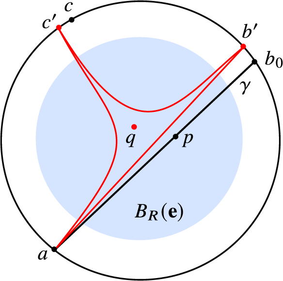
Figure 1 $p \in \pi (a,b,c)$
is close to any point q of
$p \in \pi (a,b,c)$
is close to any point q of $\pi (a, b', c')$
.
$\pi (a, b', c')$
.
We claim q is close to p. To see this, we first show p is within $2\delta $
of any geodesic from a to
$2\delta $
of any geodesic from a to $b'$
. Fix such a geodesic
$b'$
. Fix such a geodesic $[a,b']$
, and geodesics
$[a,b']$
, and geodesics $[b_0, b']$
and
$[b_0, b']$
and $[b_0, a]$
. Since
$[b_0, a]$
. Since $p \in B_R(\mathbf {e})$
, it lies distance at least
$p \in B_R(\mathbf {e})$
, it lies distance at least $10 \delta $
from any point on
$10 \delta $
from any point on $[b_0, b]$
. Also, we have that p lies within
$[b_0, b]$
. Also, we have that p lies within $\delta $
of some point on
$\delta $
of some point on $[b_0,a]$
, so by
$[b_0,a]$
, so by $\delta $
-thinness, p is distance at most
$\delta $
-thinness, p is distance at most $2\delta $
from a point on
$2\delta $
from a point on $[a,b']$
.
$[a,b']$
.
Repeating this argument with $c'$
in place of
$c'$
in place of $b'$
shows that p is within
$b'$
shows that p is within $2\delta $
of any geodesic from a to
$2\delta $
of any geodesic from a to $c'$
. A slight modification shows that p is within
$c'$
. A slight modification shows that p is within $3\delta $
of any geodesic
$3\delta $
of any geodesic $[b',c']$
, as follows: Considering a quadrilateral with sides
$[b',c']$
, as follows: Considering a quadrilateral with sides $[b_0, c]$
,
$[b_0, c]$
, $[c, c']$
,
$[c, c']$
, $[b', c']$
, and
$[b', c']$
, and $[b_0, b']$
, we know that p is within
$[b_0, b']$
, we know that p is within $\delta $
of some point on
$\delta $
of some point on $[b_0, c]$
and this must lie within
$[b_0, c]$
and this must lie within $2\delta $
of a point on
$2\delta $
of a point on $[b', c']$
since the other two sides are each distance at least
$[b', c']$
since the other two sides are each distance at least $10\delta $
from p. Thus,
$10\delta $
from p. Thus, $p \in \pi _{3\delta }(a,b',c')$
, and of course q lies in this set as well.
$p \in \pi _{3\delta }(a,b',c')$
, and of course q lies in this set as well.
By Lemma 2.5, $\pi _{3\delta }(a,b,c)$
has diameter at most
$\pi _{3\delta }(a,b,c)$
has diameter at most $Q(3\delta )$
. In particular,
$Q(3\delta )$
. In particular, $d_{\Gamma }(p,q)\le Q(3\delta )$
. Since
$d_{\Gamma }(p,q)\le Q(3\delta )$
. Since $q\in S(a,\theta )$
, this shows the second inclusion.
$q\in S(a,\theta )$
, this shows the second inclusion.
We will now combine this work with Lemma 2.12 to prove Proposition 6.6. We will actually prove the following slightly stronger statement.
Proposition 6.11. If $S(a,\theta ) \neq \emptyset $
, then
$S(a,\theta ) \neq \emptyset $
, then $S(a,\theta )$
is Hausdorff distance less than
$S(a,\theta )$
is Hausdorff distance less than $3H+6\delta +1$
from a geodesic
$3H+6\delta +1$
from a geodesic $\gamma $
with one endpoint at a.
$\gamma $
with one endpoint at a.
If in addition $L_a\cap Y_\theta \cap \sigma (D_0)$
is nonempty, then
$L_a\cap Y_\theta \cap \sigma (D_0)$
is nonempty, then $\gamma $
joins a to a point
$\gamma $
joins a to a point $e^+$
so that
$e^+$
so that $({e^+}\,|\,{\theta })_{\mathbf {e}} \ge R-(4H + 11\delta )$
.
$({e^+}\,|\,{\theta })_{\mathbf {e}} \ge R-(4H + 11\delta )$
.
Proof. We first verify the hypotheses of Lemma 2.12 for the set $S = S(a,\theta )\cap G$
(recall that G is canonically identified with the vertices of
$S = S(a,\theta )\cap G$
(recall that G is canonically identified with the vertices of $\Gamma $
). By Corollary 5.5,
$\Gamma $
). By Corollary 5.5, $\pi $
is surjective, so for each
$\pi $
is surjective, so for each $s\in \mathcal {S}$
, we can choose some
$s\in \mathcal {S}$
, we can choose some $b_s, c_s$
so that
$b_s, c_s$
so that $\sigma (a,b_s,c_s) \in L_a\cap Y_\theta $
and
$\sigma (a,b_s,c_s) \in L_a\cap Y_\theta $
and $s\in \pi (a,b_s,c_s)$
. Since
$s\in \pi (a,b_s,c_s)$
. Since $\pi ^{-1}(\mathbf {e})\subset D_0$
, the point
$\pi ^{-1}(\mathbf {e})\subset D_0$
, the point $\sigma (a,b_s,c_s)$
lies in
$\sigma (a,b_s,c_s)$
lies in $\sigma (s\cdot D_0)\cap L_a\cap Y_\theta $
. Left translating by
$\sigma (s\cdot D_0)\cap L_a\cap Y_\theta $
. Left translating by $s^{-1}$
, we have
$s^{-1}$
, we have
 $$\begin{align*}(s^{-1}a,s^{-1}b_s,s^{-1}c_s)\in \sigma(D_0)\cap L_{s^{-1}a}\cap Y_{\rho(s^{-1})\theta}.\end{align*}$$
Let $\hat {\gamma }_s$
be any biinfinite geodesic from
$\hat {\gamma }_s$
be any biinfinite geodesic from $s^{-1}a$
to
$s^{-1}a$
to $s^{-1}b_s$
. Lemma 6.10 implies
$s^{-1}b_s$
. Lemma 6.10 implies
 $$\begin{align*}s^{-1}S\cap B_R(\mathbf{e})\subset N_H(\hat{\gamma}_s),\mbox{ and } \hat{\gamma}_s\cap B_R(\mathbf{e})\subset N_H(S).\end{align*}$$
Setting $\gamma _s$
equal to
$\gamma _s$
equal to $s \cdot \hat {\gamma }_s$
, we find that
$s \cdot \hat {\gamma }_s$
, we find that
 $$\begin{align*}S\cap B_R(s)\subset N_H(\gamma_s),\mbox{ and } \gamma_s\cap B_R(s)\subset N_H(S).\end{align*}$$
Now fix any $\frac {R}{4}$
–connected component
$\frac {R}{4}$
–connected component $S_0$
of S so that we may apply Lemma 2.12 (we will see later that S is
$S_0$
of S so that we may apply Lemma 2.12 (we will see later that S is $\frac {R}{4}$
–connected, so in fact
$\frac {R}{4}$
–connected, so in fact $S_0 = S$
). The paragraph above shows that all the hypotheses of Lemma 2.12 hold for
$S_0 = S$
). The paragraph above shows that all the hypotheses of Lemma 2.12 hold for $S_0$
, so we conclude that there is a biinfinite geodesic
$S_0$
, so we conclude that there is a biinfinite geodesic $\gamma $
with
$\gamma $
with $d_{\mathrm {Haus}}(\gamma ,S_0) \le 3H + 6\delta $
.
$d_{\mathrm {Haus}}(\gamma ,S_0) \le 3H + 6\delta $
.
We next claim that one of the endpoints of $\gamma $
is a. We argue by contradiction. Using
$\gamma $
is a. We argue by contradiction. Using $\delta $
–slimness of ideal triangles, there is a point
$\delta $
–slimness of ideal triangles, there is a point $p\in \gamma $
so that p is within
$p\in \gamma $
so that p is within $2\delta $
of any geodesic joining a to any endpoint of
$2\delta $
of any geodesic joining a to any endpoint of $\gamma $
. Since
$\gamma $
. Since $S_0$
is Hausdorff distance at most
$S_0$
is Hausdorff distance at most $3H + 6\delta $
from
$3H + 6\delta $
from $\gamma $
, there is some
$\gamma $
, there is some $s\in S_0$
so that
$s\in S_0$
so that $d_{\Gamma }(s,p)\le 3H + 6\delta $
. Now
$d_{\Gamma }(s,p)\le 3H + 6\delta $
. Now $\gamma _s$
has an endpoint at a, and we have
$\gamma _s$
has an endpoint at a, and we have $\gamma _s\cap B_R(s)\subset N_H(S)$
. From the inclusions
$\gamma _s\cap B_R(s)\subset N_H(S)$
. From the inclusions $S\cap B_R(s)\subset N_H(\gamma _s),\mbox { and } \gamma _s\cap B_R(s)\subset N_H(S)$
and the inequality
$S\cap B_R(s)\subset N_H(\gamma _s),\mbox { and } \gamma _s\cap B_R(s)\subset N_H(S)$
and the inequality $6H < \frac {R}{4}$
, we conclude that
$6H < \frac {R}{4}$
, we conclude that $N_H(\gamma _s) \cap S \subset S_0$
. Choosing
$N_H(\gamma _s) \cap S \subset S_0$
. Choosing $x\in \gamma _s$
at distance
$x\in \gamma _s$
at distance $\frac {R}{2}$
from s, in the direction of a, we find some point
$\frac {R}{2}$
from s, in the direction of a, we find some point $s'\in S_0$
with
$s'\in S_0$
with $d_{\Gamma }(x,s')\le H$
. See Figure 2 for a schematic. By repeated applications of the triangle inequality, one can easily show that this
$d_{\Gamma }(x,s')\le H$
. See Figure 2 for a schematic. By repeated applications of the triangle inequality, one can easily show that this $s'$
is further than
$s'$
is further than $3H + 6\delta $
from
$3H + 6\delta $
from $\gamma $
, a contradiction.
$\gamma $
, a contradiction.
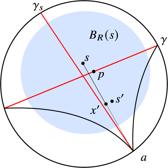
Figure 2 $\gamma $
and
$\gamma $
and $\gamma _s$
should both be close to
$\gamma _s$
should both be close to $S_0$
on the shaded region
$S_0$
on the shaded region $B_R(s)$
, giving a contradiction if a is not an endpoint of
$B_R(s)$
, giving a contradiction if a is not an endpoint of $\gamma $
.
$\gamma $
.
We now argue that $S = S_0$
. To see this, suppose that
$S = S_0$
. To see this, suppose that $S_1$
were some other component. We may apply the same argument to
$S_1$
were some other component. We may apply the same argument to $S_1$
to produce a biinfinite geodesic
$S_1$
to produce a biinfinite geodesic $\gamma _1$
. The geodesics
$\gamma _1$
. The geodesics $\gamma $
and
$\gamma $
and $\gamma _1$
share an endpoint a, and so contain points within
$\gamma _1$
share an endpoint a, and so contain points within $\delta $
of one another. This implies that
$\delta $
of one another. This implies that $S_0$
and
$S_0$
and $S_1$
contain points within
$S_1$
contain points within $6H + 13\delta < \frac {R}{4}$
of one another, so they cannot be different
$6H + 13\delta < \frac {R}{4}$
of one another, so they cannot be different $\frac {R}{4}$
–connected components.
$\frac {R}{4}$
–connected components.
We have established the first conclusion, since $d_{\mathrm {Haus}}(S,S(a,\theta ))\le 1$
.
$d_{\mathrm {Haus}}(S,S(a,\theta ))\le 1$
.
Now we suppose that $s\in S$
is in
$s\in S$
is in $\bar \pi (\sigma (D_0)\cap L_a\cap Y_\theta )$
. By Lemma 6.8, we may take s to be in
$\bar \pi (\sigma (D_0)\cap L_a\cap Y_\theta )$
. By Lemma 6.8, we may take s to be in $\bar \pi ((a,b,c),b)$
for some
$\bar \pi ((a,b,c),b)$
for some $b\in B_\epsilon (\theta )$
. We can therefore take
$b\in B_\epsilon (\theta )$
. We can therefore take $\gamma _s$
in the first part of this argument to be a geodesic joining a to b. The second conclusion of Lemma 2.12 implies that
$\gamma _s$
in the first part of this argument to be a geodesic joining a to b. The second conclusion of Lemma 2.12 implies that $({e^+}\,|\,{b})_{s}\ge R-(4H + 10\delta )$
, where
$({e^+}\,|\,{b})_{s}\ge R-(4H + 10\delta )$
, where $e^+$
is the endpoint of
$e^+$
is the endpoint of $\gamma $
which is not equal to a. We thus have
$\gamma $
which is not equal to a. We thus have
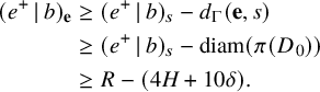 $$ \begin{align*} ({e^+}\,|\,{b})_{\mathbf{e}} & \ge ({e^+}\,|\,{b})_{s} - d_{\Gamma}(\mathbf{e},s)\\ & \ge ({e^+}\,|\,{b})_{s} - \mathrm{diam} (\pi(D_0)) \\ & \ge R - (4H + 10\delta) .\end{align*} $$
The first condition on $\epsilon $
in Lemma 6.3 implies that
$\epsilon $
in Lemma 6.3 implies that $({b}\,|\,{\theta })_{\mathbf {e}}\ge R$
. We have
$({b}\,|\,{\theta })_{\mathbf {e}}\ge R$
. We have
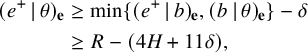 $$ \begin{align*} ({e^+}\,|\,{\theta})_{\mathbf{e}}& \ge \min\{ ({e^+}\,|\,{b})_{\mathbf{e}}, ({b}\,|\,{\theta})_{\mathbf{e}}\} - \delta\\ & \ge R - (4H + 11\delta), \end{align*} $$
establishing the last claim of the proposition.
7 The endpoint map
To summarize the results of the previous section, for each pair $a, \theta \in \partial G \times \partial G$
so that
$a, \theta \in \partial G \times \partial G$
so that $L_a \cap Y_\theta \neq \emptyset $
, there is a geodesic in
$L_a \cap Y_\theta \neq \emptyset $
, there is a geodesic in $\Gamma $
at (uniformly) bounded Hausdorff distance from
$\Gamma $
at (uniformly) bounded Hausdorff distance from $S(a,\theta ) = \overline {\pi } (L_a \cap Y_\theta )$
, with one endpoint equal to a. Say this geodesic is shadowed by
$S(a,\theta ) = \overline {\pi } (L_a \cap Y_\theta )$
, with one endpoint equal to a. Say this geodesic is shadowed by $S(a, \theta )$
, and orient it so that the negative endpoint is a. Any two biinfinite geodesics shadowed by
$S(a, \theta )$
, and orient it so that the negative endpoint is a. Any two biinfinite geodesics shadowed by $S(a,\theta )$
are bounded Hausdorff distance from each other, so they have the same endpoints in
$S(a,\theta )$
are bounded Hausdorff distance from each other, so they have the same endpoints in $\partial G$
. This gives us positive and negative “endpoint maps”
$\partial G$
. This gives us positive and negative “endpoint maps” $e^+$
and
$e^+$
and $e^-$
assigning to each pair
$e^-$
assigning to each pair $(a, \theta )$
, where
$(a, \theta )$
, where $L_a \cap Y_\theta \neq \emptyset $
the positive and negative endpoints of the shadowed geodesic. For any such
$L_a \cap Y_\theta \neq \emptyset $
the positive and negative endpoints of the shadowed geodesic. For any such $(a,\theta )$
, we have
$(a,\theta )$
, we have $e^-(a, \theta ) = a$
and
$e^-(a, \theta ) = a$
and $e^+(a, \theta ) \neq a$
. Furthermore, the equivariance property in Proposition 3.2 implies that for any
$e^+(a, \theta ) \neq a$
. Furthermore, the equivariance property in Proposition 3.2 implies that for any $g \in G$
, we have
$g \in G$
, we have
 $$\begin{align*}g S(a,\theta) = S(g a, \rho(g) \theta ) = \overline{\pi} (L_{ga} \cap Y_{\rho(g) \theta}). \end{align*}$$
This implies the following equivariance of the positive endpoint map
 $$ \begin{align} g \cdot e^+(a, \theta) = e^+(ga, \rho(g) \theta). \end{align} $$
Here, and in what follows, we will frequently omit $\rho _0$
from the notation when it is clear that we are referring to the natural action of G on its boundary. Thus, we will write
$\rho _0$
from the notation when it is clear that we are referring to the natural action of G on its boundary. Thus, we will write $ga$
rather than
$ga$
rather than $\rho _0(g)a$
when a is a boundary point. For
$\rho _0(g)a$
when a is a boundary point. For $x \in X$
, we also write
$x \in X$
, we also write $gx$
for its image under the standard action of
$gx$
for its image under the standard action of $g \in G$
on
$g \in G$
on $X \subset \Xi $
.
$X \subset \Xi $
.
We will first establish continuity of the positive endpoint map on a large set, then use it to define a semiconjugacy.
7.1 Continuity
Proposition 7.1 (Continuity in
$a, \theta $
over
$D_1$
)


Suppose $a_0, \theta _0 \in \partial G \times \partial G$
is such that there exists c with
$a_0, \theta _0 \in \partial G \times \partial G$
is such that there exists c with $(a_0, \theta _0, c) \in D_1$
. Then the map
$(a_0, \theta _0, c) \in D_1$
. Then the map $(a, \theta ) \mapsto e^+(a, \theta )$
is continuous at
$(a, \theta ) \mapsto e^+(a, \theta )$
is continuous at $(a_0, \theta _0)$
.
$(a_0, \theta _0)$
.
Proposition 7.1 will be a quick consequence of the following technical lemma.
Lemma 7.2. Suppose $L_{a_0} \cap Y_{\theta _0}$
is nonempty. For any
$L_{a_0} \cap Y_{\theta _0}$
is nonempty. For any $r>0$
, there is a neighborhood
$r>0$
, there is a neighborhood $N = N(r)$
of
$N = N(r)$
of $(a_0,\theta _0)\in \partial G \times \partial G$
so that if
$(a_0,\theta _0)\in \partial G \times \partial G$
so that if $(a , \theta ) \in N$
, then
$(a , \theta ) \in N$
, then $B_r(\mathbf {e})\cap S(a_0,\theta _0)$
lies in the
$B_r(\mathbf {e})\cap S(a_0,\theta _0)$
lies in the $\mathrm {diam}(\pi (D_1))$
–neighborhood of
$\mathrm {diam}(\pi (D_1))$
–neighborhood of $S(a,\theta )$
.
$S(a,\theta )$
.
The main idea behind the proof of Lemma 7.2 comes from the proof of Lemma 6.8, and the fact that the fixed point property used there is stable under small perturbations of the map $f_{a,c,\theta }$
.
$f_{a,c,\theta }$
.
Proof of Lemma 7.2
If $B_r(\mathbf {e})\cap S(a_0,\theta _0)$
is empty, there is nothing to show, so we suppose
$B_r(\mathbf {e})\cap S(a_0,\theta _0)$
is empty, there is nothing to show, so we suppose $B_r(\mathbf {e})\cap S(a_0,\theta _0)$
is nonempty. Let
$B_r(\mathbf {e})\cap S(a_0,\theta _0)$
is nonempty. Let $K\subset X$
be the closure of
$K\subset X$
be the closure of $\pi ^{-1}(B_r(\mathbf {e}))$
.
$\pi ^{-1}(B_r(\mathbf {e}))$
.
Recall from Notation 6.7 that $f_{a,c,\theta }$
denotes the map
$f_{a,c,\theta }$
denotes the map $x \mapsto f_\theta (a, x, c)$
, and recall that
$x \mapsto f_\theta (a, x, c)$
, and recall that $D_0\subset D_1$
has the following properties
$D_0\subset D_1$
has the following properties
-
1.
$X \subset GD_0$
-
2. For any
$(a,b,c)\in D_0$
, the set
$B_{\epsilon _1}(a) \times B_{\epsilon _1}(b) \times B_{\epsilon _1}(c)$
is contained in
$D_1$
(see Lemma 6.2.(4)).


Recall also that $\epsilon _1> \epsilon _2 > 2 \epsilon $
.
$\epsilon _1> \epsilon _2 > 2 \epsilon $
.
We cover $\sigma (K) \cap (L_{a_0} \cap Y_{\theta _0})$
with translates of
$\sigma (K) \cap (L_{a_0} \cap Y_{\theta _0})$
with translates of $D_0$
, as follows. Since K is compact, there are finitely many elements
$D_0$
, as follows. Since K is compact, there are finitely many elements $g_1, g_2, \ldots g_k \in G$
so that
$g_1, g_2, \ldots g_k \in G$
so that
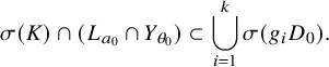 $$\begin{align*}\sigma(K) \cap (L_{a_0} \cap Y_{\theta_0}) \subset \bigcup_{i=1}^k \sigma(g_i D_0). \end{align*}$$
By deleting elements from the list if necessary, we may assume
 $$\begin{align*}\sigma(g_i D_0) \cap \left(L_{a_0} \cap Y_{\theta_0} \right) \neq \emptyset\end{align*}$$
for each i.
Our next goal is to show that, for each i, the projection of the larger translate $g_iD_1$
to the Cayley graph contains a point of
$g_iD_1$
to the Cayley graph contains a point of $S(a, \theta )$
, provided that
$S(a, \theta )$
, provided that $(a, \theta )$
is chosen close enough to
$(a, \theta )$
is chosen close enough to $(a_0,\theta _0)$
. Here, “close enough” depends on the set K and hence on the constant r.
$(a_0,\theta _0)$
. Here, “close enough” depends on the set K and hence on the constant r.
Translating back to $D_0$
, for each i, we have
$D_0$
, for each i, we have $\sigma (D_0) \cap \left ( L_{g_i^{-1}a_0} \cap Y_{\rho (g_i)^{-1}\theta _0} \right ) \neq \emptyset $
. Let
$\sigma (D_0) \cap \left ( L_{g_i^{-1}a_0} \cap Y_{\rho (g_i)^{-1}\theta _0} \right ) \neq \emptyset $
. Let $b_i, c_i \in \partial G$
be such that
$b_i, c_i \in \partial G$
be such that
 $$\begin{align*}\left( ( g_i^{-1}a_0, b_i, c_i ), b_i \right) \in \sigma(D_0) \cap \left( L_{g_i^{-1} a_0} \cap Y_{\rho(g_i)^{-1}\theta_0} \right). \end{align*}$$
Because $ \left ( g_i^{-1}a_0, b_i, c_i \right ) \in D_0 \subset D_2$
, Definition 6.4, Item (4) implies that
$ \left ( g_i^{-1}a_0, b_i, c_i \right ) \in D_0 \subset D_2$
, Definition 6.4, Item (4) implies that
 $$\begin{align*}b_i = f_{\rho(g_i)^{-1}\theta_0}(g_i^{-1}a_0, b_i, c_i) \in B_{\epsilon}(\rho(g_i)^{-1}\theta_0). \end{align*}$$
Hence, $d_{\mathrm {vis}}(b_i,\rho (g_i)^{-1}\theta _0) < \epsilon $
, and so
$d_{\mathrm {vis}}(b_i,\rho (g_i)^{-1}\theta _0) < \epsilon $
, and so $(g_i^{-1}a_0, \rho (g_i)^{-1}\theta _0, c_i ) \in D_1$
.
$(g_i^{-1}a_0, \rho (g_i)^{-1}\theta _0, c_i ) \in D_1$
.
Let ${p_i} = \rho (g_i)^{-1}\theta _0$
. By Item (2) of Definition 6.4, there is some s
${p_i} = \rho (g_i)^{-1}\theta _0$
. By Item (2) of Definition 6.4, there is some s $c^{\prime }_i \in B_\epsilon (c_i)$
so that
$c^{\prime }_i \in B_\epsilon (c_i)$
so that $ \{a_i\} \times B_{\epsilon _2}({p_i}) \times \{c^{\prime }_i\}$
lies in the interior of X. Furthermore, by Lemma 6.3, Item (ϵ2), there is a closed contractible set
$ \{a_i\} \times B_{\epsilon _2}({p_i}) \times \{c^{\prime }_i\}$
lies in the interior of X. Furthermore, by Lemma 6.3, Item (ϵ2), there is a closed contractible set $B_{p_i} \subset \partial G$
with
$B_{p_i} \subset \partial G$
with $B_\epsilon ({p_i}) \subset B_{p_i} \subset B_{\epsilon _2}({p_i})$
, and
$B_\epsilon ({p_i}) \subset B_{p_i} \subset B_{\epsilon _2}({p_i})$
, and
 $$\begin{align*}f_{g_i^{-1} a_0, c^{\prime}_i, {p_i}}(B_{\epsilon_2}({p_i})) \subset B_\epsilon({p_i}),\end{align*}$$
so $f_{g_i^{-1} a_0, c^{\prime }_i, {p_i}}$
has a fixed point in
$f_{g_i^{-1} a_0, c^{\prime }_i, {p_i}}$
has a fixed point in $B_\epsilon ({p_i})$
. The property of taking the compact set
$B_\epsilon ({p_i})$
. The property of taking the compact set $B_{p_i}$
into the open ball
$B_{p_i}$
into the open ball $B_\epsilon ({p_i})$
is open (in the compact-open topology on continuous maps), so also holds for any map sufficiently close to
$B_\epsilon ({p_i})$
is open (in the compact-open topology on continuous maps), so also holds for any map sufficiently close to $f_{g_i^{-1} a_0, c^{\prime }_i, {p_i}}$
, provided the map is defined on
$f_{g_i^{-1} a_0, c^{\prime }_i, {p_i}}$
, provided the map is defined on $B_{p_i}$
. Recall that the domain of definition of
$B_{p_i}$
. Recall that the domain of definition of $f_{x,y,z}$
is the set
$f_{x,y,z}$
is the set $\{ w \mid (x, w, z) \in X \}$
. Thus, if a function
$\{ w \mid (x, w, z) \in X \}$
. Thus, if a function $f_{x,y,z}$
is defined on a set
$f_{x,y,z}$
is defined on a set $\{x\} \times B_{\epsilon _2}({p_i}) \times \{z\}$
contained in the interior of X, and
$\{x\} \times B_{\epsilon _2}({p_i}) \times \{z\}$
contained in the interior of X, and $B_{\epsilon _2}({p_i}) \supset B_{p_i}$
, then for all sufficiently close
$B_{\epsilon _2}({p_i}) \supset B_{p_i}$
, then for all sufficiently close $x', y', z'$
, the function
$x', y', z'$
, the function $f_{x',y', z'}$
will be defined on
$f_{x',y', z'}$
will be defined on $B_{p_i}$
as well. Additionally, the functions
$B_{p_i}$
as well. Additionally, the functions $f_{x,y,z}$
vary continuously in the arguments
$f_{x,y,z}$
vary continuously in the arguments $(x,y,z)$
. Thus, we may take a neighborhood
$(x,y,z)$
. Thus, we may take a neighborhood $N_i$
of
$N_i$
of $(a_0, \theta _0)$
, such that for each
$(a_0, \theta _0)$
, such that for each $(a, \theta ) \in N_i$
,
$(a, \theta ) \in N_i$
,
-
1. the map
$f_{g_i^{-1} a, c^{\prime }_i, \rho (g_i)^{-1}\theta }$
is defined on
$B_{p_i}$
-
2. the map
$f_{g_i^{-1} a, c^{\prime }_i, \rho (g_i)^{-1}\theta }$
has a fixed point contained in
$B_\epsilon ({p_i})$
; and -
3.
$d_{\mathrm {vis}}(g_i^{-1} a,g_i^{-1} a_0)< \epsilon _1$
.


Set $N = \bigcap _{i=1}^k N_i$
. Thus, for any
$N = \bigcap _{i=1}^k N_i$
. Thus, for any $(a, \theta ) \in N$
, each of the sets
$(a, \theta ) \in N$
, each of the sets $L_{g_i^{-1}(a)} \cap Y_{\rho (g_i)^{-1}\theta }$
contains a point
$L_{g_i^{-1}(a)} \cap Y_{\rho (g_i)^{-1}\theta }$
contains a point $\sigma (g_i^{-1} a, z_i, c^{\prime }_i)$
, where
$\sigma (g_i^{-1} a, z_i, c^{\prime }_i)$
, where $z_i \in B_\epsilon ({p_i})$
. In particular, we have
$z_i \in B_\epsilon ({p_i})$
. In particular, we have
 $$ \begin{align*} & d_{\mathrm{vis}}(g_i^{-1} a, g_i^{-1} a_0)< \epsilon_1 \text{ and } \\ & d_{\mathrm{vis}}(z_i,b_i)\le 2\epsilon <\epsilon_1. \end{align*} $$
Since $(g_i^{-1} a_0,b_i,c_i)\in D_0$
, this means that
$(g_i^{-1} a_0,b_i,c_i)\in D_0$
, this means that $(g_i^{-1} a, z_i, c^{\prime }_i)\in D_1$
. Multiplying on the left by
$(g_i^{-1} a, z_i, c^{\prime }_i)\in D_1$
. Multiplying on the left by $g_i$
, we obtain
$g_i$
, we obtain $(a,g_iz_i,g_ic^{\prime }_i) \in g_iD_1$
and
$(a,g_iz_i,g_ic^{\prime }_i) \in g_iD_1$
and $\sigma (a,g_iz_i,g_ic^{\prime }_i)\in L_{a}\cap Y_{\theta }$
, so the intersection
$\sigma (a,g_iz_i,g_ic^{\prime }_i)\in L_{a}\cap Y_{\theta }$
, so the intersection
 $$\begin{align*}\sigma(g_i D_1) \cap (L_a\cap Y_\theta) \end{align*}$$
is nonempty for each of the elements $g_i$
. Projecting to the Cayley graph, we have
$g_i$
. Projecting to the Cayley graph, we have $B_r(\mathbf {e})\cap S(a_0,\theta _0)$
contained in the
$B_r(\mathbf {e})\cap S(a_0,\theta _0)$
contained in the $\mathrm {diam}(\pi (D_1))$
–neighborhood of
$\mathrm {diam}(\pi (D_1))$
–neighborhood of $S(a,\theta )$
, which proves the lemma.
$S(a,\theta )$
, which proves the lemma.
Proof of Proposition 7.1 from Lemma 7.2
Suppose $(a_0, \theta _0) \in \partial G \times \partial G$
is such that there exists c with
$(a_0, \theta _0) \in \partial G \times \partial G$
is such that there exists c with $(a_0, \theta _0, c) \in D_1$
. Then by Lemma 6.8,
$(a_0, \theta _0, c) \in D_1$
. Then by Lemma 6.8, $L_{a_0} \cap Y_{\theta _0}$
contains a point of
$L_{a_0} \cap Y_{\theta _0}$
contains a point of $\sigma (D_2)$
, so is nonempty. Lemma 7.2 states that, given
$\sigma (D_2)$
, so is nonempty. Lemma 7.2 states that, given $r>0$
, there is a neighborhood N of
$r>0$
, there is a neighborhood N of $(a_0,\theta _0)$
so that if
$(a_0,\theta _0)$
so that if $(a , \theta ) \in N$
, then
$(a , \theta ) \in N$
, then $B_r(\mathbf {e})\cap S(a_0,\theta _0)$
lies in the
$B_r(\mathbf {e})\cap S(a_0,\theta _0)$
lies in the $\mathrm {diam}(\pi (D_1))$
–neighborhood of
$\mathrm {diam}(\pi (D_1))$
–neighborhood of $S(a,\theta )$
. By Proposition 6.11, both
$S(a,\theta )$
. By Proposition 6.11, both $S(a_0,\theta _0)$
and
$S(a_0,\theta _0)$
and $S(a,\theta )$
are Hausdorff distance at most
$S(a,\theta )$
are Hausdorff distance at most $3H+6\delta +1$
from some biinfinite geodesic, so these geodesics will
$3H+6\delta +1$
from some biinfinite geodesic, so these geodesics will $2(3H + 6\delta + 1)+ \mathrm {diam}(\pi (D_1))$
fellow-travel each other over a compact set, which can be taken as large as we wish by taking r large. This gives continuity.
$2(3H + 6\delta + 1)+ \mathrm {diam}(\pi (D_1))$
fellow-travel each other over a compact set, which can be taken as large as we wish by taking r large. This gives continuity.
We now establish continuity of a similar positive endpoint map defined everywhere on X. Since f is a homeomorphism and the sets $X\times \{\theta \}$
partition
$X\times \{\theta \}$
partition $X\times \partial G$
, so do their images
$X\times \partial G$
, so do their images $Y_\theta $
. Likewise, the sets
$Y_\theta $
. Likewise, the sets $L_a$
give a partition of
$L_a$
give a partition of $\sigma (X)\subset X\times \partial G$
, so for each
$\sigma (X)\subset X\times \partial G$
, so for each $x \in X$
, there exists a unique
$x \in X$
, there exists a unique $a(x)$
and
$a(x)$
and $\theta (x)$
, such that
$\theta (x)$
, such that $\sigma (x) \in L_{a(x)} \cap Y_{\theta (x)}$
. Note if
$\sigma (x) \in L_{a(x)} \cap Y_{\theta (x)}$
. Note if $x = (a,b,c)$
, then
$x = (a,b,c)$
, then $a(x) =a$
. We have a sequence of maps:
$a(x) =a$
. We have a sequence of maps:
 $$ \begin{align} x = (a,b,c) \mapsto ((a, b, c), b) \mapsto (a, \theta(x)) \mapsto e^+(a, \theta(x)). \end{align} $$
Proposition 7.3 (Continuity on X)
Let $\mathcal {E}^+(x)= e^+(a(x), \theta (x))$
be the map given by the composition in (13). Then
$\mathcal {E}^+(x)= e^+(a(x), \theta (x))$
be the map given by the composition in (13). Then $\mathcal {E}^+$
is continuous on all of X.
$\mathcal {E}^+$
is continuous on all of X.
Proof. Equivariance of each map in the composition implies that we have the equivariance property
 $$\begin{align*}\mathcal{E}^+(g x) = \mathcal{E}^+(g a(x),\rho(g)\theta(x)) .\end{align*}$$
It therefore suffices to check continuity of the composition above on the set $D_0 \cap X$
containing a fundamental domain for the action of G on X.
$D_0 \cap X$
containing a fundamental domain for the action of G on X.
By definition, the section $\sigma $
is continuous. For the second map in (13), note that
$\sigma $
is continuous. For the second map in (13), note that $\theta (x)$
is simply projection onto the second coordinate of
$\theta (x)$
is simply projection onto the second coordinate of $f^{-1}(\sigma (x)) \in X \times \partial G$
. Since
$f^{-1}(\sigma (x)) \in X \times \partial G$
. Since $f^{-1}$
is a homeomorphism of
$f^{-1}$
is a homeomorphism of $X \times \partial G$
, its projection
$X \times \partial G$
, its projection $\theta (x)$
is continuous. Finally, Proposition 7.1 says that
$\theta (x)$
is continuous. Finally, Proposition 7.1 says that $(a, \theta (a,b,c)) \mapsto e^+(a, \theta )$
is continuous for
$(a, \theta (a,b,c)) \mapsto e^+(a, \theta )$
is continuous for $(a,b,c) \in D_1$
.
$(a,b,c) \in D_1$
.
Going forward, we will abuse notation and often think of $\mathcal {E}^+$
as a map defined on
$\mathcal {E}^+$
as a map defined on $\sigma (X)$
, via the identification of X with
$\sigma (X)$
, via the identification of X with $\sigma (X)$
.
$\sigma (X)$
.
7.2 Proof of Theorem 1.1
Using the work above, we may now conclude the proof of our main theorem. First recall the statement.
Theorem 1.1 (Topological stability)
Let G be a hyperbolic group with sphere boundary. Then the action of G on $\partial G$
is topologically stable. More precisely, given any neighborhood V of the identity in the space of continuous self-maps of
$\partial G$
is topologically stable. More precisely, given any neighborhood V of the identity in the space of continuous self-maps of $S^n$
, there exists a neighborhood U of the standard boundary action in
$S^n$
, there exists a neighborhood U of the standard boundary action in $\mathrm {Hom}(G, \mathrm {Homeo}(S^n))$
, such that any representation in U has
$\mathrm {Hom}(G, \mathrm {Homeo}(S^n))$
, such that any representation in U has $\rho _0$
as a factor, with semiconjugacy contained in V.
$\rho _0$
as a factor, with semiconjugacy contained in V.
Our neighborhood $U = \mathcal U(V)$
was determined by our desired lower bound
$U = \mathcal U(V)$
was determined by our desired lower bound $C_V$
on Gromov products when we set our conventions in Section 6.1. In this section, we show that
$C_V$
on Gromov products when we set our conventions in Section 6.1. In this section, we show that $e^+(a,\theta )$
is (locally) a function only of
$e^+(a,\theta )$
is (locally) a function only of $\theta $
, hence can be thought of as a map from
$\theta $
, hence can be thought of as a map from $\partial G$
to
$\partial G$
to $\partial G$
. We will then show that this map has the properties of the desired semiconjugacy between
$\partial G$
. We will then show that this map has the properties of the desired semiconjugacy between $\rho _0$
and
$\rho _0$
and $\rho $
.
$\rho $
.
Lemma 7.4 (
$e^+$
is locally a function of
$\theta $
)


Let $\theta \in \partial G$
, and let
$\theta \in \partial G$
, and let $\{a_t\mid t \in [0,1]\}$
be a path in
$\{a_t\mid t \in [0,1]\}$
be a path in $\partial G$
so that
$\partial G$
so that $e^+(a_t, \theta )$
is defined and continuous at all points. Then
$e^+(a_t, \theta )$
is defined and continuous at all points. Then $e^+(a_t, \theta )$
is constant.
$e^+(a_t, \theta )$
is constant.
Proof. We argue by contradiction. Suppose we have such a path where $e^+$
is nonconstant. Truncating and reparameterizing, we may suppose that
$e^+$
is nonconstant. Truncating and reparameterizing, we may suppose that
-
1.
$e^+(a_t,\theta )$
is not locally constant at
$t=0$
, -
2. for all
$t\in [0,1]$
,
$a_t \neq e^+(a_0,\theta )$
, and -
3.
$e^+(a_1,\theta )\ne e^+(a_0,\theta )$
.


The second item can be ensured by taking any sufficiently short path that is nonconstant at $0$
, since
$0$
, since $e^+(a, \theta ) \neq a$
holds for all
$e^+(a, \theta ) \neq a$
holds for all $a, \theta $
.
$a, \theta $
.
Since G acts on $\partial G$
as a uniform convergence action (see Proposition 2.2), the point
$\partial G$
as a uniform convergence action (see Proposition 2.2), the point $e^+(a_0,\theta )$
is a conical limit point, so there exists a sequence
$e^+(a_0,\theta )$
is a conical limit point, so there exists a sequence $\{g_i\} \subset G$
and points
$\{g_i\} \subset G$
and points $p \neq q \in \partial G$
, such that
$p \neq q \in \partial G$
, such that $g_i e^+(a_0,\theta ) \to p$
and
$g_i e^+(a_0,\theta ) \to p$
and $g_i z \to q$
for all
$g_i z \to q$
for all $z \in \partial G - \{e^+(a_0,\theta )\}$
. Modifying the sequence
$z \in \partial G - \{e^+(a_0,\theta )\}$
. Modifying the sequence $\{g_i\}$
if needed by postcomposing with some fixed
$\{g_i\}$
if needed by postcomposing with some fixed $g \in G$
, we may also assume there exists c with
$g \in G$
, we may also assume there exists c with $(p,q,c) \in D_0$
. In particular, this implies that
$(p,q,c) \in D_0$
. In particular, this implies that $B_\epsilon (p)\cap B_\epsilon (q) = \emptyset $
. Since
$B_\epsilon (p)\cap B_\epsilon (q) = \emptyset $
. Since $\partial G$
is compact, we may assume by passing to a subsequence that
$\partial G$
is compact, we may assume by passing to a subsequence that $\rho (g_i)\theta $
converges to some point
$\rho (g_i)\theta $
converges to some point $\theta _\infty \in \partial G$
.
$\theta _\infty \in \partial G$
.
For i large enough, $g_i \cdot e^+(a_1, \theta ) \in B_{\epsilon /2}(q)$
and
$g_i \cdot e^+(a_1, \theta ) \in B_{\epsilon /2}(q)$
and $g_i \cdot e^+(a_0, \theta ) \in B_{\epsilon /2}(p)$
. Thus, for each sufficiently large i, there exists
$g_i \cdot e^+(a_0, \theta ) \in B_{\epsilon /2}(p)$
. Thus, for each sufficiently large i, there exists $t_i$
, such that
$t_i$
, such that $p_i:= g_i \cdot e^+(a_{t_i}, \theta )$
is visual distance exactly
$p_i:= g_i \cdot e^+(a_{t_i}, \theta )$
is visual distance exactly $\epsilon $
from p. Since the arc
$\epsilon $
from p. Since the arc $a_t$
does not meet
$a_t$
does not meet $e^+(a_0,\theta )$
, we have
$e^+(a_0,\theta )$
, we have $g_ia_t\in B_{\epsilon }(q)$
for all t and sufficiently large i. See Figure 3 for a schematic illustration. Consider the sets
$g_ia_t\in B_{\epsilon }(q)$
for all t and sufficiently large i. See Figure 3 for a schematic illustration. Consider the sets $g_i S(a_{t_i},\theta ) = S(g_i(a_{t_i}), \rho (g_i)(\theta ))$
. Recall by (12), we have
$g_i S(a_{t_i},\theta ) = S(g_i(a_{t_i}), \rho (g_i)(\theta ))$
. Recall by (12), we have
 $$\begin{align*}e^+(g_i a_t, \rho(g_i) \theta) = g_i \cdot e^+(a_t, \theta). \end{align*}$$
This implies that the geodesics shadowed by the sets $S(g_i(a_{t_i}), \rho (g_i)(\theta ))$
all pass through some compact subset of the Cayley graph
$S(g_i(a_{t_i}), \rho (g_i)(\theta ))$
all pass through some compact subset of the Cayley graph $\Gamma $
, and so the sets themselves all meet some compact
$\Gamma $
, and so the sets themselves all meet some compact $K\subset X$
.
$K\subset X$
.
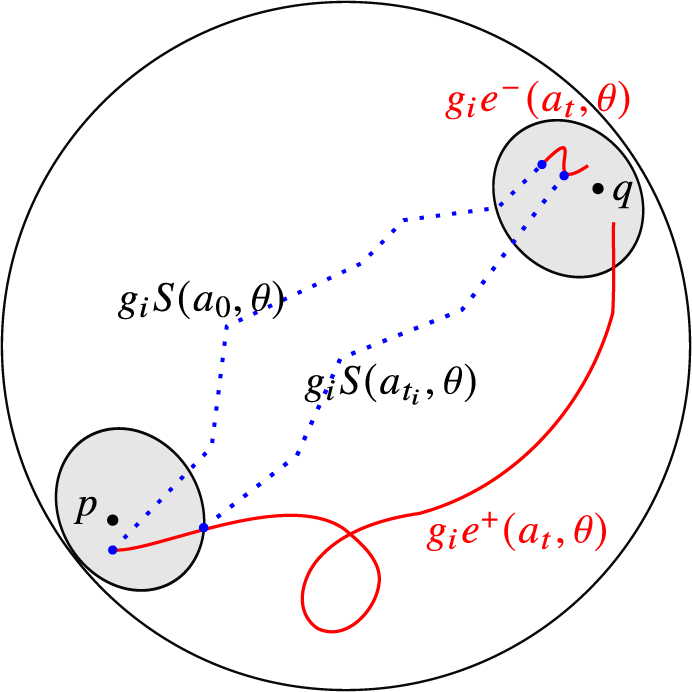
Figure 3 Paths of endpoints (red/solid line) on $\partial G = \partial \Gamma $
and associated near-geodesic sets in
$\partial G = \partial \Gamma $
and associated near-geodesic sets in $\Gamma $
(blue/dotted) with endpoints in the
$\Gamma $
(blue/dotted) with endpoints in the $\epsilon $
-balls about p and q.
$\epsilon $
-balls about p and q.
For each i, fix a point $y_i \in L_{g_i a_{t_i}} \cap Y_{\rho (g_i)(\theta )} \cap K$
. After passing to a further subsequence, the points
$y_i \in L_{g_i a_{t_i}} \cap Y_{\rho (g_i)(\theta )} \cap K$
. After passing to a further subsequence, the points $y_i$
converge to some
$y_i$
converge to some $y_\infty \in K$
. Now
$y_\infty \in K$
. Now $g_i a_{t_i} \to q$
and
$g_i a_{t_i} \to q$
and $\rho (g_i)(\theta ) \to \theta _\infty $
, so
$\rho (g_i)(\theta ) \to \theta _\infty $
, so $y_\infty \in L_q \cap Y_{\theta _\infty } \cap K$
. Using the notation from Proposition 7.3, continuity of positive endpoints implies that
$y_\infty \in L_q \cap Y_{\theta _\infty } \cap K$
. Using the notation from Proposition 7.3, continuity of positive endpoints implies that $\mathcal {E}^+(y_\infty ) = \lim _{n \to \infty } \mathcal {E}^+(y_i)$
which is by construction some point at distance
$\mathcal {E}^+(y_\infty ) = \lim _{n \to \infty } \mathcal {E}^+(y_i)$
which is by construction some point at distance $\epsilon $
from p.
$\epsilon $
from p.
Now consider instead the constant sequence $t = 0$
instead of
$t = 0$
instead of $t_i$
. By the same reasoning, for i sufficiently large,
$t_i$
. By the same reasoning, for i sufficiently large, $L_{g_i a_{0}} \cap Y_{\rho (g_i)(\theta )}$
will contain a point
$L_{g_i a_{0}} \cap Y_{\rho (g_i)(\theta )}$
will contain a point $z_i$
in K. After passing to a subsequence, these converge to a point
$z_i$
in K. After passing to a subsequence, these converge to a point $z_\infty \in L_q \cap Y_{\theta _\infty } \cap K$
. By continuity of
$z_\infty \in L_q \cap Y_{\theta _\infty } \cap K$
. By continuity of $\mathcal {E}^+$
, we have
$\mathcal {E}^+$
, we have $\mathcal {E}^+(z_\infty ) = \lim _{n \to \infty } \mathcal {E}^+(z_i) = p$
. Thus, we have found two points,
$\mathcal {E}^+(z_\infty ) = \lim _{n \to \infty } \mathcal {E}^+(z_i) = p$
. Thus, we have found two points, $y_\infty $
and
$y_\infty $
and $z_\infty $
, both in
$z_\infty $
, both in $Y_{\theta _\infty } \cap L_q$
with different positive endpoints
$Y_{\theta _\infty } \cap L_q$
with different positive endpoints $\mathcal {E}^+(z_\infty ) \ne \mathcal {E}^+(y_\infty )$
. This directly contradicts Proposition 6.11, and this contradiction concludes the proof.
$\mathcal {E}^+(z_\infty ) \ne \mathcal {E}^+(y_\infty )$
. This directly contradicts Proposition 6.11, and this contradiction concludes the proof.
Recall that Item (6) from Lemma 6.2 says that, if $(a, \theta , c)$
and
$(a, \theta , c)$
and $(a', \theta , c')$
lie in
$(a', \theta , c')$
lie in $D_1$
, then there exists a path
$D_1$
, then there exists a path $a_t$
with
$a_t$
with $a_0 = a$
and
$a_0 = a$
and $a_1 = a'$
and a point
$a_1 = a'$
and a point $c"$
, such that
$c"$
, such that $(a_t, \theta , c") \in D_1$
for all t. Proposition 7.1 says that the map
$(a_t, \theta , c") \in D_1$
for all t. Proposition 7.1 says that the map $e^+(a_t, \theta )$
is therefore continuous at each point, and thus by Lemma 7.4, we conclude it is constant. In summary, we have the following.
$e^+(a_t, \theta )$
is therefore continuous at each point, and thus by Lemma 7.4, we conclude it is constant. In summary, we have the following.
Corollary 7.5. If $(a, \theta , c)$
and
$(a, \theta , c)$
and $(a', \theta , c')$
lie in
$(a', \theta , c')$
lie in $D_1$
, then
$D_1$
, then $e^+(a, \theta ) = e^+(a', \theta )$
.
$e^+(a, \theta ) = e^+(a', \theta )$
.
Definition 7.6. Define $h:S^{n-1} \to S^{n-1}$
by
$h:S^{n-1} \to S^{n-1}$
by $h(\theta ) = e^+(a, \theta )$
, where a is any point, such that there exists c with
$h(\theta ) = e^+(a, \theta )$
, where a is any point, such that there exists c with $(a, \theta , c) \in D_0$
.
$(a, \theta , c) \in D_0$
.
Note that h is defined everywhere, and is continuous by the continuity of $e^+(a, \theta )$
given by Proposition 7.1. It remains to check that h satisfies the other properties of the semiconjugacy required to prove Theorem 1.1. The second point in Proposition 6.11 states that
$e^+(a, \theta )$
given by Proposition 7.1. It remains to check that h satisfies the other properties of the semiconjugacy required to prove Theorem 1.1. The second point in Proposition 6.11 states that $({h(\theta )}\,|\,{\theta })_{\mathbf {e}} \ge R-(4H + 11\delta )$
. Our choice of R in Lemma 6.2 (⋆⋆) implies that
$({h(\theta )}\,|\,{\theta })_{\mathbf {e}} \ge R-(4H + 11\delta )$
. Our choice of R in Lemma 6.2 (⋆⋆) implies that $({h(\theta )}\,|\,{\theta })_{\mathbf {e}} \ge C_V$
, satisfying (†) as desired, and showing that h lies in our chosen neighborhood V. This neighborhood contains only degree one maps, so h is surjective.
$({h(\theta )}\,|\,{\theta })_{\mathbf {e}} \ge C_V$
, satisfying (†) as desired, and showing that h lies in our chosen neighborhood V. This neighborhood contains only degree one maps, so h is surjective.
We now check equivariance. Let g be an element of the generating set $\mathcal {S} \cup \mathcal {S}^{-1}$
used in the definition of
$\mathcal {S} \cup \mathcal {S}^{-1}$
used in the definition of $\Gamma $
, and let
$\Gamma $
, and let $\theta $
be given. Choose a so that
$\theta $
be given. Choose a so that $(a, \theta , c) \in D_0$
. We have
$(a, \theta , c) \in D_0$
. We have
 $$\begin{align*}\rho_0(g) h(\theta) = g e^+(a, \theta) = e^+(g a, \rho(g) \theta) .\end{align*}$$
By definition of $D_{\frac {1}{2}}$
, and our conditions on
$D_{\frac {1}{2}}$
, and our conditions on $\rho $
, we have
$\rho $
, we have $(ga, g\theta , gc) \in D_{\frac {1}{2}}$
. By definition of
$(ga, g\theta , gc) \in D_{\frac {1}{2}}$
. By definition of $D_1$
, and Item (3) of Definition 6.4 which defines the neighborhood
$D_1$
, and Item (3) of Definition 6.4 which defines the neighborhood $\mathcal U(V)$
, we then have
$\mathcal U(V)$
, we then have $(ga, \rho (g)\theta , gc) \in D_1$
. Thus, by Corollary 7.5,
$(ga, \rho (g)\theta , gc) \in D_1$
. Thus, by Corollary 7.5, $e^+(ga, \rho (g) \theta , gc) = e^+(a', \rho (g)\theta , c')$
for any choice of
$e^+(ga, \rho (g) \theta , gc) = e^+(a', \rho (g)\theta , c')$
for any choice of $a'$
and
$a'$
and $c'$
, such that
$c'$
, such that $(a', \rho (g)\theta , c') \in D_0$
, thus giving
$(a', \rho (g)\theta , c') \in D_0$
, thus giving
 $$ \begin{align} \rho_0(g) h(\theta) = h(\rho(g) \theta) \end{align} $$
for all $\theta \in \partial G$
. Since (14) holds for generators of G, it holds, inductively, for all elements
$\theta \in \partial G$
. Since (14) holds for generators of G, it holds, inductively, for all elements $g \in G$
. This shows that h is a semiconjugacy in the specified neighborhood of the identity map of
$g \in G$
. This shows that h is a semiconjugacy in the specified neighborhood of the identity map of $S^n$
, completing the proof of the theorem.
$S^n$
, completing the proof of the theorem.
Acknowledgements
K.M. was partially supported by NSF grant DMS 1844516 and a Sloan fellowship. J.M. was partially supported by Simons Collaboration Grant #524176.
Competing interest
The authors have no competing interest to declare.


 Open access