


1 Introduction
Spherical designs are point sets in the sphere $\mathbb {S} ^d = \{x\in \mathbb {R} ^{d+1}: \|x\|=1\}$
that yield exact quadrature rules with constant weights for polynomial spaces. Thus, a finite set
$\mathbb {S} ^d = \{x\in \mathbb {R} ^{d+1}: \|x\|=1\}$
that yield exact quadrature rules with constant weights for polynomial spaces. Thus, a finite set $X_t\subseteq \mathbb {S} ^d$
is a t-design (or
$X_t\subseteq \mathbb {S} ^d$
is a t-design (or $X_t$
consists of t-design points) if for every algebraic polynomial f in
$X_t$
consists of t-design points) if for every algebraic polynomial f in $d+1$
variables of (total) degree t, one has
$d+1$
variables of (total) degree t, one has
 $$ \begin{align} \frac{1}{|X_t|} \sum_{x\in X_t} f(x) = \int _{\mathbb{S} ^d} f \,. \end{align} $$
This concept plays an important role in numerical analysis, approximation theory and many related fields, and the theory, construction and applications of spherical designs has become a highly developed art. See [10, 40, 41] and [5, 21, 42, 48] for a sample of papers on spherical t-design points. In particular, the existence of asymptotically optimal t-design points in the d-sphere has long been an open problem and has eventually been proved by Bondarenko, Radchenko and Viazovska in [Reference Bondarenko, Radchenko and Viazovska3].
In this paper, we study a variation where points are replaced by curves. The goal is again to obtain quadrature formulas along curves in the sphere that are exact for polynomials of a given degree. The central notion is the definition of a t-design curve. Precisely, a closed, piecewise smooth curve $\gamma : [0,1] \to \mathbb {S} ^d$
with at most finitely many self intersections and with arc length
$\gamma : [0,1] \to \mathbb {S} ^d$
with at most finitely many self intersections and with arc length $\ell (\gamma )$
is called a t-design curve in
$\ell (\gamma )$
is called a t-design curve in $\mathbb {S} ^d$
if the line integral integrates exactly all algebraic polynomials in
$\mathbb {S} ^d$
if the line integral integrates exactly all algebraic polynomials in $d+1$
variables of degree t,
$d+1$
variables of degree t,
 $$ \begin{align} \frac{1}{\ell (\gamma )} \int _\gamma f = \int _{\mathbb{S} ^d} f\,. \end{align} $$
The use of curves instead of point evaluations in definition (2) is motivated by numerous analogous applications of curves for the collection and processing of data on the sphere. Here is a short list of applications of curves in a similar spirit: Low-discrepancy curves were discussed in [Reference Ramamoorthy, Rajagopal and Wenzel35] as an efficient coverage of space with applications in robotics. See also the textbook [Reference LaValle30] on robotics, where curves are derived for motion planning to obtain an optimal path under several side constraints. Space-filling curves are used as dimensionality reduction tools in optimization, image processing and deep learning cf. [20, 8, 44]. Curves are applied in [Reference Ehler, Gräf, Neumayer and Steidl14] to approximate probability measures. The concept of principal curves is discussed in [Reference Hauberg24, Reference Hastie and Stuetzle23, Reference Kegl, Krzyzak, Linder and Zeger28, Reference Lee, Kim and Oh31] to best fit given data. In another statistical context, the information tuning curve quantifies discriminatory abilities of populations of neurons [Reference Ringach37, Reference Kang, Shapley and Sompolinsky27]. Motivated by more geometric questions, length and thickness of ropes on spheres are studied in [Reference Gerlach and von der Mosel17, Reference Gerlach and von der Mosel18] as variants of packing problems. In the context of optimization problems, the shortest closed space curve to inspect a sphere is determined in [Reference Ghomi and Wenk19]; variations are discussed in [Reference Zalgaller50]. Energy minimization and geometric arrangements in biophysics lead to optimality questions of knots and ropes [Reference Cantarella, Kusner and Sullivan7, Reference O’Hara33, Reference Yu, Schumacher and Crane49]. In mobile sampling, curve trajectories provide sampling sets that enable efficient signal reconstruction [Reference Benedetto and Wu2, Reference Jaming, Negreira and Romero25, Reference Gröchenig, Romero, Unnikrishnan and Vetterli22, Reference Jaye and Mitkovski26, Reference Unnikrishnan and Vetterli46, Reference Unnikrishnan and Vetterli45, Reference Rashkovskii, Ulanovskii and Zlotnikov36].
Our goal is to study integration on the sphere by using information along closed curves rather than point evaluations. The new notion of t-design curves in (2) addresses exact integration on the sphere along curves and the related problem of the exact reconstruction of bandlimited functions on the sphere. The pertinent questions of t-design curves on spheres are similar to those of spherical t-design points.
Problem $(A)$
: What is the minimal (order of the) arc length of a t-design curve?
$(A)$
: What is the minimal (order of the) arc length of a t-design curve?
Problem $(B)$
: Do t-design curves exist on
$(B)$
: Do t-design curves exist on $\mathbb {S} ^d$
for all
$\mathbb {S} ^d$
for all $t\in \mathbb {N}$
?
$t\in \mathbb {N}$
?
Problem $(C)$
: If yes, are there t-design curves on
$(C)$
: If yes, are there t-design curves on $\mathbb {S} ^d$
achieving the optimal order of arc length?
$\mathbb {S} ^d$
achieving the optimal order of arc length?
Problem $(D)$
: Provide explicit constructions of t-design curves.
$(D)$
: Provide explicit constructions of t-design curves.
The answers to the analogous questions for t-design points have a long history and culminate in the solution of the Korevaar-Meyers conjecture by Bondarenko, Radchenko and Viazovska [Reference Bondarenko, Radchenko and Viazovska3] mentioned above.
Our program is to make a first attempt at these questions for t-design curves on d-spheres. We will offer answers to $(A)$
and
$(A)$
and $(B)$
and give a solution of problem
$(B)$
and give a solution of problem $(C)$
on the sphere
$(C)$
on the sphere $\mathbb {S} ^2$
. As a contribution to Problem
$\mathbb {S} ^2$
. As a contribution to Problem $(D)$
, we will construct some examples of smooth t-design curves for small degrees t.
$(D)$
, we will construct some examples of smooth t-design curves for small degrees t.
Results. In the following, we denote the space of algebraic polynomials of $d+1$
real variables of (total) degree t by
$d+1$
real variables of (total) degree t by $\Pi _t$
. As a necessary condition for the length of a t-design curve, we obtain the following answer to Problem
$\Pi _t$
. As a necessary condition for the length of a t-design curve, we obtain the following answer to Problem $(A)$
.
$(A)$
.
Theorem 1.1. Assume that a piecewise smooth, closed curve $\gamma : [0,1] \to \mathbb {S} ^d$
satisfies
$\gamma : [0,1] \to \mathbb {S} ^d$
satisfies
 $$\begin{align*}\frac{1}{\ell (\gamma )} \int _\gamma f = \int _{\mathbb{S} ^d} f \qquad \text{ for all } \, f \in \Pi _t \,. \end{align*}$$
Then its length is bounded from below by
 $$\begin{align*}\ell (\gamma ) \geq C_d t^{d-1 } \end{align*}$$
with some constant $C_d>0$
that may depend on the dimension d but is independent of t and
$C_d>0$
that may depend on the dimension d but is independent of t and $\gamma $
.
$\gamma $
.
By comparison, a spherical t-design requires $|X_t| \asymp t^d$
points [Reference de la Harpe and Pache9, Reference Seidel40, Reference Delsarte, Goethals and Seidel10].Footnote
1
$|X_t| \asymp t^d$
points [Reference de la Harpe and Pache9, Reference Seidel40, Reference Delsarte, Goethals and Seidel10].Footnote
1
The next challenge is to prove the existence of t-design curves that match the asymptotic order $ t^{d-1}$
. For the unit sphere in
$ t^{d-1}$
. For the unit sphere in $\mathbb {R}^3$
, we succeeded in proving the existence. This solves Problem
$\mathbb {R}^3$
, we succeeded in proving the existence. This solves Problem $(C)$
for
$(C)$
for $\mathbb {S} ^2$
.
$\mathbb {S} ^2$
.
Theorem 1.2. In $\mathbb {S} ^2$
there exists a sequence of t-design curves
$\mathbb {S} ^2$
there exists a sequence of t-design curves $\left (\gamma _t\right )_{t\in \mathbb {N}}$
with length
$\left (\gamma _t\right )_{t\in \mathbb {N}}$
with length $\ell (\gamma _t) \asymp t $
.
$\ell (\gamma _t) \asymp t $
.
Note that even for $d=2$
, the corresponding problem of the existence of spherical t-designs points was solved only in 2011 [Reference Bondarenko, Radchenko and Viazovska3]. In our proof, we will make substantial use of the result from [Reference Bondarenko, Radchenko and Viazovska3]. In dimension
$d=2$
, the corresponding problem of the existence of spherical t-designs points was solved only in 2011 [Reference Bondarenko, Radchenko and Viazovska3]. In our proof, we will make substantial use of the result from [Reference Bondarenko, Radchenko and Viazovska3]. In dimension $d\geq 3$
, we prove the existence of t-design curves. This is a solution to Problem
$d\geq 3$
, we prove the existence of t-design curves. This is a solution to Problem $(B)$
.
$(B)$
.
Theorem 1.3. In $\mathbb {S}^d$
for
$\mathbb {S}^d$
for $d\geq 3$
, there exists a sequence of t-design curves
$d\geq 3$
, there exists a sequence of t-design curves $\left (\gamma _t\right )_{t\in \mathbb {N}}$
, such that
$\left (\gamma _t\right )_{t\in \mathbb {N}}$
, such that $\ell (\gamma _t) \lesssim t^{d(d-1)/2}$
.
$\ell (\gamma _t) \lesssim t^{d(d-1)/2}$
.
This asymptotic order does not match our lower bounds for $d\geq 3$
in Theorem 1.1. In the analogous problem of t-design points, our Theorem 1.3 corresponds to the upper bounds of Korevaar and Meyers [Reference Korevaar and Meyers29] from 1993. It remains an interesting challenge to derive the existence of t-design curves on
$d\geq 3$
in Theorem 1.1. In the analogous problem of t-design points, our Theorem 1.3 corresponds to the upper bounds of Korevaar and Meyers [Reference Korevaar and Meyers29] from 1993. It remains an interesting challenge to derive the existence of t-design curves on $\mathbb {S} ^d$
that match the bounds of Theorem 1.1.
$\mathbb {S} ^d$
that match the bounds of Theorem 1.1.
The existence theorems are constructive only in part, as they are based on the non-constructive results of Bondarenko, Radchenko and Viazovska [Reference Bondarenko, Radchenko and Viazovska3]. We will describe a procedure that associates to every set of t-design points in $\mathbb {S} ^d$
a corresponding t-design curve. This part is constructive, and the result is a closed, piecewise smooth curve that consists of arcs of Euclidean circles (by a circle in
$\mathbb {S} ^d$
a corresponding t-design curve. This part is constructive, and the result is a closed, piecewise smooth curve that consists of arcs of Euclidean circles (by a circle in $\mathbb {S} ^d$
, we mean a circle in the intersection of a
$\mathbb {S} ^d$
, we mean a circle in the intersection of a $2$
-dimensional subspace of
$2$
-dimensional subspace of $\mathbb {R} ^{d+1}$
with
$\mathbb {R} ^{d+1}$
with $\mathbb {S} ^d$
).
$\mathbb {S} ^d$
).
As a small contribution to Problem $(D)$
, we will discuss some explicit constructions of smooth t-design curves for very low polynomial degrees (
$(D)$
, we will discuss some explicit constructions of smooth t-design curves for very low polynomial degrees ( $t=1,2,3$
). Explicit constructions of t-design points and curves remain a difficult problem with many open threads.
$t=1,2,3$
). Explicit constructions of t-design points and curves remain a difficult problem with many open threads.
Mobile sampling. Mobile sampling refers to the approximation or reconstruction of a function from its values along a curve [Reference Unnikrishnan and Vetterli45, Reference Unnikrishnan and Vetterli46]. The rationale for this mode of data acquisition is the small number of required sensors. Sampling a function along a curve requires only one sensor, whereas the sampling at a point set (e.g., t-design points) requires many sensors. In engineering applications, it is natural to assume that the function f to be sampled is bandlimited on $\mathbb {R} ^d$
(i.e., the support of the Fourier transform
$\mathbb {R} ^d$
(i.e., the support of the Fourier transform $\hat {f}$
is compact).
$\hat {f}$
is compact).
Transferred to the sphere $\mathbb {S} ^d$
, a function on the sphere is bandlimited if it is a polynomial restricted to the sphere. Its degree is a measure for the bandwidth. A typical and natural scenario for mobile sampling on the sphere would be the surveillance of meteorological or geophysical data along airplane routes. The goal would be to reconstruct the complete data globally, which means literally on the entire ‘globe’ (i.e.,
$\mathbb {S} ^d$
, a function on the sphere is bandlimited if it is a polynomial restricted to the sphere. Its degree is a measure for the bandwidth. A typical and natural scenario for mobile sampling on the sphere would be the surveillance of meteorological or geophysical data along airplane routes. The goal would be to reconstruct the complete data globally, which means literally on the entire ‘globe’ (i.e., $\mathbb {S} ^2$
). The connection between t-design curves and mobile sampling on the sphere is explained in the following statement.
$\mathbb {S} ^2$
). The connection between t-design curves and mobile sampling on the sphere is explained in the following statement.
Corollary 1.4. Let $\gamma $
be a
$\gamma $
be a $2t$
-design curve on
$2t$
-design curve on $\mathbb {S} ^d$
and f a polynomial of degree t. Then
$\mathbb {S} ^d$
and f a polynomial of degree t. Then
 $$ \begin{align} \frac{1}{\ell (\gamma )} \int _\gamma |f|^2 = \int _{\mathbb{S} ^d} |f|^2 \,. \end{align} $$
Furthermore, f is uniquely determined by its values along $\gamma $
.
$\gamma $
.
Clearly, (3) follows immediately from the assumption because $f \in \Pi _t$
implies that
$f \in \Pi _t$
implies that $|f|^2 \in \Pi _{2t}$
. The uniqueness and an explicit reconstruction formula will be derived in Section 7.
$|f|^2 \in \Pi _{2t}$
. The uniqueness and an explicit reconstruction formula will be derived in Section 7.
We also discuss some elementary consequences of t-design curves on the sphere in high-dimensional Euclidean quadrature. Generalized Gauss-Laguerre quadrature combined with spherical t-design curves lead to exact integration of polynomials of total degree t with respect to the measure $\mathrm {e}^{-\|x\|}\mathrm {d}x$
on
$\mathrm {e}^{-\|x\|}\mathrm {d}x$
on $\mathbb {R}^d$
.
$\mathbb {R}^d$
.
Methods. Both Theorems 1.1 and 1.2 are based on the existence of optimal t-design points. An immediate guess would be to connect t-design points along geodesic arcs in $\mathbb {S} ^d$
and hope that a suitable order of points would yield a t-design curve. As there are
$\mathbb {S} ^d$
and hope that a suitable order of points would yield a t-design curve. As there are $O (t^d)$
points in a t-design with a distance
$O (t^d)$
points in a t-design with a distance $O (t^{-1})$
to the nearest neighbor, the solution of the traveling salesman problem would lead to a curve of the desired length
$O (t^{-1})$
to the nearest neighbor, the solution of the traveling salesman problem would lead to a curve of the desired length $O (t^{d-1})$
[Reference Ehler, Gräf, Neumayer and Steidl14, Lemma 3]. However, so far this idea has not been fruitful, and we do not know how such a path would yield exact quadrature.
$O (t^{d-1})$
[Reference Ehler, Gräf, Neumayer and Steidl14, Lemma 3]. However, so far this idea has not been fruitful, and we do not know how such a path would yield exact quadrature.
Our idea is to connect the point evaluation $f\to f(x), x\in \mathbb {S} ^d$
to an integral over the boundary of a spherical cap by means of a formula of Samko [Reference Samko39]. In
$f\to f(x), x\in \mathbb {S} ^d$
to an integral over the boundary of a spherical cap by means of a formula of Samko [Reference Samko39]. In $\mathbb {S} ^2$
, the boundary of a spherical cap is a circle, and thus the union of such circles with centers at t-design points yields a first quadrature rule. To generate a single closed curve from this union of circles, we invoke some combinatorial arguments from graph theory, such as spanning trees and Eulerian paths. The extension to higher dimensions is by induction on the dimension d. Here we need some additional properties from spherical geometry.
$\mathbb {S} ^2$
, the boundary of a spherical cap is a circle, and thus the union of such circles with centers at t-design points yields a first quadrature rule. To generate a single closed curve from this union of circles, we invoke some combinatorial arguments from graph theory, such as spanning trees and Eulerian paths. The extension to higher dimensions is by induction on the dimension d. Here we need some additional properties from spherical geometry.
Outlook. Spherical t-design points have proved a rich field of research with deep mathematical questions. The new theory of t-design curves offers a similarly rich playground for both challenging mathematics and for the investigation of associated numerical and computational questions and applications.
On the mathematical side, the most immediate question is the existence of t-design curves of asymptotically optimal length in $\mathbb {S}^d$
for
$\mathbb {S}^d$
for $d\geq 3$
. Another direction is the exploration of t-design curves on general compact Riemannian manifolds (extending the work on t-design points in [Reference Ehler, Etayo, Gariboldi, Gigante and Peter13, Reference Etayo, Marzo and Ortega-Cerdà15, Reference Gariboldi and Gigante16]). Theorem 1.1 on the lower bound on the length of a t-design curve carries over to the manifold setting, but all constructive aspects are wide open.
$d\geq 3$
. Another direction is the exploration of t-design curves on general compact Riemannian manifolds (extending the work on t-design points in [Reference Ehler, Etayo, Gariboldi, Gigante and Peter13, Reference Etayo, Marzo and Ortega-Cerdà15, Reference Gariboldi and Gigante16]). Theorem 1.1 on the lower bound on the length of a t-design curve carries over to the manifold setting, but all constructive aspects are wide open.
Next, one might want to impose additional conditions on the curves. Our construction yields piecewise smooth, closed curves with finitely many corners and self-intersections. For aesthetical reasons, one might want t-design curves to be smooth and simple (i.e., without corners and self-intersections). So far, we know such examples only for degrees $t\leq 3 $
on
$t\leq 3 $
on $\mathbb {S} ^2$
. Other aspects to be considered might be curvature, contractibility (or other homotopy constraints) or the ratio between inner and outer area for closed curves on surfaces. At this time, we are far from understanding any of these questions.
$\mathbb {S} ^2$
. Other aspects to be considered might be curvature, contractibility (or other homotopy constraints) or the ratio between inner and outer area for closed curves on surfaces. At this time, we are far from understanding any of these questions.
The outline is as follows: In Section 2, we introduce the concept of t-design curves in $\mathbb {S}^d$
, and we derive asymptotic lower bounds on the curves’ length. Smooth spherical t-design curves in
$\mathbb {S}^d$
, and we derive asymptotic lower bounds on the curves’ length. Smooth spherical t-design curves in $\mathbb {S}^2$
for
$\mathbb {S}^2$
for $t=1,2,3$
are provided in Section 3. Section 4 is dedicated to some preparations for our two main theorems. The first one on the existence of asymptotically optimal t-design curves in
$t=1,2,3$
are provided in Section 3. Section 4 is dedicated to some preparations for our two main theorems. The first one on the existence of asymptotically optimal t-design curves in $\mathbb {S}^2$
is derived in Section 5. The existence of t-design curves in
$\mathbb {S}^2$
is derived in Section 5. The existence of t-design curves in $\mathbb {S}^d$
is proved in Section 6. In Section 7, we briefly discuss the use of t-design curves in mobile sampling and for high-dimensional quadrature on
$\mathbb {S}^d$
is proved in Section 6. In Section 7, we briefly discuss the use of t-design curves in mobile sampling and for high-dimensional quadrature on $\mathbb {R}^d$
.
$\mathbb {R}^d$
.
2 From points to curves
We denote the collection of classical polynomials of total degree at most $t\in \mathbb {N}$
in
$t\in \mathbb {N}$
in $d+1$
variables on
$d+1$
variables on $\mathbb {R}^{d+1}$
by
$\mathbb {R}^{d+1}$
by $\Pi _t$
. Each
$\Pi _t$
. Each $f\in \Pi _t$
can be evaluated on the unit sphere
$f\in \Pi _t$
can be evaluated on the unit sphere $\mathbb {S}^d=\{x\in \mathbb {R}^{d+1}:\|x\|=1\}$
. We always use the normalized surface measure, so that
$\mathbb {S}^d=\{x\in \mathbb {R}^{d+1}:\|x\|=1\}$
. We always use the normalized surface measure, so that $\int _{\mathbb {S}^d} 1 = 1$
. The (rotation-) invariant metric on
$\int _{\mathbb {S}^d} 1 = 1$
. The (rotation-) invariant metric on $\mathbb {S} ^d$
is
$\mathbb {S} ^d$
is
 $$ \begin{align} \operatorname{\mathrm{dist}}(x,y) = \arccos \langle x,y \rangle\,. \end{align} $$
It measures the length of the geodesic arc connecting x and y on $\mathbb {S}^d$
.
$\mathbb {S}^d$
.
2.1 t-design points
For $t\in \mathbb {N}$
, a finite set
$t\in \mathbb {N}$
, a finite set $X\subset \mathbb {S}^d$
is called t-design points (or simply t-design) in
$X\subset \mathbb {S}^d$
is called t-design points (or simply t-design) in $\mathbb {S}^d$
if
$\mathbb {S}^d$
if
 $$ \begin{align} \frac{1}{|X|}\sum_{x\in X} f(x) = \int_{\mathbb{S}^d} f ,\qquad \forall f\in\Pi_t. \end{align} $$
We call $(X_t)_{t\in \mathbb {N}}$
a sequence of t-design points in
$(X_t)_{t\in \mathbb {N}}$
a sequence of t-design points in $\mathbb {S}^d$
if each
$\mathbb {S}^d$
if each $X_t$
is a t-design for
$X_t$
is a t-design for $t\in \mathbb {N}$
.
$t\in \mathbb {N}$
.
It turns out that each sequence $(X_t)_{t\in \mathbb {N}}$
of t-design points in
$(X_t)_{t\in \mathbb {N}}$
of t-design points in $\mathbb {S}^d$
must satisfy
$\mathbb {S}^d$
must satisfy
 $$ \begin{align} |X_t|\gtrsim t^d,\qquad t\in\mathbb{N}, \end{align} $$
where the constant may depend on d but is independent of t, cf. [Reference Breger, Ehler and Gräf6]. A sequence of t-design points $(X_t)_{t\in \mathbb {N}}$
in
$(X_t)_{t\in \mathbb {N}}$
in $\mathbb {S}^d$
is called asymptotically optimal if
$\mathbb {S}^d$
is called asymptotically optimal if
 $$ \begin{align*} |X_t|\asymp t^d, \qquad t\in\mathbb{N}. \end{align*} $$
Again, we allow the constant to depend on d. Asymptotically optimal point sequences do exist [Reference Bondarenko, Radchenko and Viazovska3, Reference Ehler, Etayo, Gariboldi, Gigante and Peter13, Reference Etayo, Marzo and Ortega-Cerdà15, Reference Gariboldi and Gigante16].
2.2 t-design curves
We now introduce a new concept by switching from points to a curve. By a curve, we mean a continuous, piecewise differentiable function $\gamma :[0,1]\rightarrow \mathbb {S}^d$
with at most finitely many self-intersections. Since the sphere is a closed manifold, we only consider closed curves.
$\gamma :[0,1]\rightarrow \mathbb {S}^d$
with at most finitely many self-intersections. Since the sphere is a closed manifold, we only consider closed curves.
We may interpret $\gamma $
as a space curve in
$\gamma $
as a space curve in $\mathbb {R}^{d+1}$
, so that its length is
$\mathbb {R}^{d+1}$
, so that its length is
 $$\begin{align*}\ell(\gamma)=\int_0^1 \|\dot{\gamma}(s)\|\mathrm{d}s, \end{align*}$$
where the speed $\|\dot {\gamma }\|$
of the curve is defined almost everywhere. The line integral is
$\|\dot {\gamma }\|$
of the curve is defined almost everywhere. The line integral is
 $$ \begin{align*} \int_{\gamma} f = \int_0^1 f(\gamma (s))\|\dot{\gamma}(s)\|\mathrm{d}s, \end{align*} $$
so that $\ell (\gamma )=\int _\gamma 1$
. Note that
$\ell (\gamma )=\int _\gamma 1$
. Note that $\int _\gamma f $
does not depend on the parametrization and orientation of the curve.
$\int _\gamma f $
does not depend on the parametrization and orientation of the curve.
In analogy to (5), we now introduce t-design curves.
Definition 2.1. For $t\in \mathbb {N}$
, we say that
$t\in \mathbb {N}$
, we say that $\gamma $
is a t-design curve in
$\gamma $
is a t-design curve in $\mathbb {S}^d$
if
$\mathbb {S}^d$
if
 $$ \begin{align} \frac{1}{\ell(\gamma)}\int_{\gamma} f = \int_{\mathbb{S}^d} f ,\qquad f\in\Pi_t. \end{align} $$
A sequence of curves $(\gamma _t)_{t\in \mathbb {N}}$
is called a sequence of t-design curves in
$(\gamma _t)_{t\in \mathbb {N}}$
is called a sequence of t-design curves in $\mathbb {S}^d$
if each
$\mathbb {S}^d$
if each $\gamma _t$
is a t-design for
$\gamma _t$
is a t-design for $t\in \mathbb {N}$
.
$t\in \mathbb {N}$
.
Analogously to (6), one now expects lower asymptotic bounds on $\ell (\gamma _t)$
; see also [Reference Ehler, Gräf, Neumayer and Steidl14, Theorem 3 in Section 5]. The following is Theorem 1.1 of the Introduction.
$\ell (\gamma _t)$
; see also [Reference Ehler, Gräf, Neumayer and Steidl14, Theorem 3 in Section 5]. The following is Theorem 1.1 of the Introduction.
Theorem 2.2. If $(\gamma _t)_{t\in \mathbb {N}}$
a sequence of t-design curves in
$(\gamma _t)_{t\in \mathbb {N}}$
a sequence of t-design curves in $\mathbb {S}^d$
, then
$\mathbb {S}^d$
, then
 $$ \begin{align} \ell(\gamma_t) \gtrsim t^{d-1},\quad t\in\mathbb{N}. \end{align} $$
Proof. We use some results from [Reference Breger, Ehler and Gräf6] and [Reference Brandolini, Choirat, Colzani, Gigante, Seri and Travaglini4]. Let $\Gamma _t=\gamma _t([0,1])$
be the trajectory of
$\Gamma _t=\gamma _t([0,1])$
be the trajectory of $\gamma _t$
. The covering radius
$\gamma _t$
. The covering radius $\rho _t$
of
$\rho _t$
of $\Gamma _t$
is defined as
$\Gamma _t$
is defined as
 $$ \begin{align} \rho_t:=\sup_{x\in\mathbb{S}^d}\left(\inf_{y\in\Gamma_t}\operatorname{\mathrm{dist}}(x,y)\right). \end{align} $$
By this definition, there is $x\in \mathbb {S}^d$
such that the closed ball
$x\in \mathbb {S}^d$
such that the closed ball $B_{\rho _t/2}(x)=\{y\in \mathbb {S}^d:\operatorname {\mathrm {dist}}(x,y)\leq \frac {\rho _t}{2}\}$
of radius
$B_{\rho _t/2}(x)=\{y\in \mathbb {S}^d:\operatorname {\mathrm {dist}}(x,y)\leq \frac {\rho _t}{2}\}$
of radius $\rho _t/2$
centered at x does not intersect
$\rho _t/2$
centered at x does not intersect $\Gamma _t$
; that is,
$\Gamma _t$
; that is,
 $$ \begin{align} B_{\rho_t/2}(x)\cap \Gamma_t = \emptyset. \end{align} $$
Let us denote the Laplace-Beltrami operator on the sphere $\mathbb {S}^d$
by
$\mathbb {S}^d$
by $\Delta $
and the identity operator by I. According to [Reference Breger, Ehler and Gräf6, Lemma 5.2 with
$\Delta $
and the identity operator by I. According to [Reference Breger, Ehler and Gräf6, Lemma 5.2 with $s=2d$
and
$s=2d$
and $p=1$
], see also [Reference Brandolini, Choirat, Colzani, Gigante, Seri and Travaglini4] for the original idea, there is a function
$p=1$
], see also [Reference Brandolini, Choirat, Colzani, Gigante, Seri and Travaglini4] for the original idea, there is a function $f_t$
supported on
$f_t$
supported on $B_{\rho _t/2}(x)$
such that
$B_{\rho _t/2}(x)$
such that
 $$ \begin{align} \|(I-\Delta)^d f_t\|_{L^1(\mathbb{S}^d)} \lesssim 1,\qquad \text{ and } \qquad \rho_t^{2d}\lesssim \int_{\mathbb{S}^d} f_t. \end{align} $$
Since (10) implies $\int _{\gamma _t} f_t = 0$
, the t-design assumption and [Reference Brandolini, Choirat, Colzani, Gigante, Seri and Travaglini4, Theorem 2.12] lead to
$\int _{\gamma _t} f_t = 0$
, the t-design assumption and [Reference Brandolini, Choirat, Colzani, Gigante, Seri and Travaglini4, Theorem 2.12] lead to
 $$ \begin{align} \left|\int_{\mathbb{S}^d} f_t\right| \lesssim t^{-2d} \|(I-\Delta)^d f_t\|_{L^1}. \end{align} $$
By combining (12) with (11), we deduce $\rho _t^{2d}\lesssim t^{-2d}$
, so that
$\rho _t^{2d}\lesssim t^{-2d}$
, so that
 $$ \begin{align} \rho_t\lesssim t^{-1}. \end{align} $$
To relate $\rho _t$
with
$\rho _t$
with $\ell (\gamma _t)$
, we apply a packing argument. Let n be the maximum number of disjoint balls of radius
$\ell (\gamma _t)$
, we apply a packing argument. Let n be the maximum number of disjoint balls of radius $2\rho _t$
in
$2\rho _t$
in $\mathbb {S}^d$
(i.e.,
$\mathbb {S}^d$
(i.e., $B_{2\rho _t}(x_j) \cap B_{2\rho _t}(x_k) = \emptyset $
for
$B_{2\rho _t}(x_j) \cap B_{2\rho _t}(x_k) = \emptyset $
for $j,k= 1, \dots , n$
with
$j,k= 1, \dots , n$
with $j\neq k$
). Then the balls
$j\neq k$
). Then the balls $B_{4\rho _t}(x_j)$
cover
$B_{4\rho _t}(x_j)$
cover $\mathbb {S}^d$
; otherwise, there is
$\mathbb {S}^d$
; otherwise, there is $x\in \mathbb {S}^d$
, such that
$x\in \mathbb {S}^d$
, such that $x\not \in \bigcup _{j=1}^n B_{4\rho _t}(x_j)$
and
$x\not \in \bigcup _{j=1}^n B_{4\rho _t}(x_j)$
and $B_{2\rho _t}(x)$
is disjoint from all
$B_{2\rho _t}(x)$
is disjoint from all $B_{2\rho _t}(x_j)$
, contradicting the maximality of n.
$B_{2\rho _t}(x_j)$
, contradicting the maximality of n.
We note that every ball $B_r(x)$
in
$B_r(x)$
in $\mathbb {S}^d $
with radius
$\mathbb {S}^d $
with radius $0<r\leq 1$
has volume
$0<r\leq 1$
has volume $\operatorname *{\mathrm {vol}}(B_r(x))\asymp r^d$
. Consequently,
$\operatorname *{\mathrm {vol}}(B_r(x))\asymp r^d$
. Consequently,
 $$ \begin{align*} 1 \leq \sum _{j=1}^n \operatorname*{\mathrm{vol}}(B_{4\rho _t}(x_j)) \lesssim n \rho _t ^d, \end{align*} $$
so that we obtain
 $$ \begin{align*} n\gtrsim \rho_t^{-d}. \end{align*} $$
This is known as the Gilbert-Varshamov bound in coding theory, cf. [Reference Barg1].
Since $B_{2\rho _t}(x_j) \cap B_{2\rho _t}(x_k) = \emptyset $
, the distance between two distinct balls
$B_{2\rho _t}(x_j) \cap B_{2\rho _t}(x_k) = \emptyset $
, the distance between two distinct balls $B_{\rho _t}(x_j)$
and
$B_{\rho _t}(x_j)$
and $B_{\rho _t}(x_k)$
is at least
$B_{\rho _t}(x_k)$
is at least $2\rho _t$
. Due to the definition of the covering radius
$2\rho _t$
. Due to the definition of the covering radius $\rho _t$
and the compactness of
$\rho _t$
and the compactness of $\Gamma _t$
and
$\Gamma _t$
and $\mathbb {S}^d$
, the trajectory
$\mathbb {S}^d$
, the trajectory $\Gamma _t$
intersects each ball
$\Gamma _t$
intersects each ball $B_{\rho _t}(x_k)$
. Therefore, the length of
$B_{\rho _t}(x_k)$
. Therefore, the length of $\gamma _t$
must satisfy
$\gamma _t$
must satisfy
 $$ \begin{align} \ell(\gamma_t) \gtrsim n \rho_t \gtrsim \rho_t^{1-d}. \end{align} $$
Since (13) is equivalent to $\rho ^{-1}_t \gtrsim t$
, the bound (14) leads to
$\rho ^{-1}_t \gtrsim t$
, the bound (14) leads to
 $$ \begin{align*} \ell(\gamma_t) \gtrsim \rho_t^{1-d} \gtrsim t^{d-1}.\\[-38pt] \end{align*} $$
The lower bound on the length of $\gamma _t$
leads to the concept of asymptotic optimality for curves.
$\gamma _t$
leads to the concept of asymptotic optimality for curves.
Definition 2.3. A sequence $(\gamma _t)_{t\in \mathbb {N}}$
of t-design curves in
$(\gamma _t)_{t\in \mathbb {N}}$
of t-design curves in $\mathbb {S}^d$
is called asymptotically optimal if
$\mathbb {S}^d$
is called asymptotically optimal if
 $$ \begin{align*} \ell(\gamma_t)\asymp t^{d-1}, \qquad t\in\mathbb{N}. \end{align*} $$
In the remainder of the paper, we study the existence of t-design curves on the sphere $\mathbb {S} ^d$
.
$\mathbb {S} ^d$
.
3 Some spherical t-design curves for small t in $\mathbb {S}^2$

Here we construct smooth t-design curves in $\mathbb {S}^2$
for
$\mathbb {S}^2$
for $t=1,2,3$
. For
$t=1,2,3$
. For $1\leq k\in \mathbb {N}$
and
$1\leq k\in \mathbb {N}$
and $a\in [0,1]$
, consider the family of curves
$a\in [0,1]$
, consider the family of curves $\gamma ^{(k,a)}:[0,1]\rightarrow \mathbb {S}^2$
given by
$\gamma ^{(k,a)}:[0,1]\rightarrow \mathbb {S}^2$
given by
 $$ \begin{align} \gamma^{(k,a)}(s):= \begin{pmatrix} a\cos(2\pi s)+(1-a)\cos(2\pi (2k-1) s)\\ a\sin(2\pi s)-(1-a)\sin(2\pi (2k-1) s)\\ 2\sqrt{a(1-a)}\sin(2\pi k s) \end{pmatrix}\,. \end{align} $$
If $k=1$
, then
$k=1$
, then $\gamma ^{(k,a)}$
describes a great circle, and it is easy to see that every great circle in
$\gamma ^{(k,a)}$
describes a great circle, and it is easy to see that every great circle in $\mathbb {S}^d$
yields a
$\mathbb {S}^d$
yields a $1$
-design. The family
$1$
-design. The family $\gamma ^{(k,a)}$
also gives rise to spherical
$\gamma ^{(k,a)}$
also gives rise to spherical $2$
-design and
$2$
-design and $3$
-design curves.
$3$
-design curves.
Proposition 3.1. The curves $\gamma ^{(k,a)}$
have the following properties:
$\gamma ^{(k,a)}$
have the following properties:
-
(i)
$\gamma ^{(k,a)}$
is a
$1$
-design curve for all
$k\in \mathbb {N} $
. -
(ii) There is
$a_2\in (\frac {1}{2},1)$
such that
$\gamma ^{(2,a_2)}$
is a
$2$
-design curve. -
(iii) For
$k\geq 3$
, there is
$a_k\in (\frac {1}{2},1)$
such that
$\gamma ^{(k,a_k)}$
is a
$3$
-design curve.


To verify Proposition 3.1, recall that the surface measure on $\mathbb {S}^2$
is normalized, so that
$\mathbb {S}^2$
is normalized, so that $\int _{\mathbb {S}^2} 1 =1$
. Due to the sphere’s symmetries, integrals over the sphere of every monomial of odd degree vanish. Moreover, when
$\int _{\mathbb {S}^2} 1 =1$
. Due to the sphere’s symmetries, integrals over the sphere of every monomial of odd degree vanish. Moreover, when $x,y,z$
denote the coordinate functions in
$x,y,z$
denote the coordinate functions in $\mathbb {R}^3$
, we have
$\mathbb {R}^3$
, we have
 $$ \begin{align} 0 &=\int_{\mathbb{S}^2}xy=\int_{\mathbb{S}^2}xz=\int_{\mathbb{S}^2}yz, \end{align} $$
 $$ \begin{align}\ \ \frac{1}{3} &= \int_{\mathbb{S}^2}x^2 = \int_{\mathbb{S}^2}y^2 = \int_{\mathbb{S}^2}z^2.\quad \end{align} $$
By definition of length, we directly observe
 $$ \begin{align} \int_{\mathbb{S}^2} 1 =1= \frac{1}{\ell(\gamma^{(k,a)})}\int_0^1\|\dot{\gamma}^{(k,a)}(s)\| \mathrm{d}s = \frac{1}{\ell(\gamma^{(k,a)})}\int_{\gamma^{(k,a)}} 1. \end{align} $$
To treat line integrals of the other monomials, will use the following lemma.
Lemma 3.2. There are real-valued coefficients $(c^{(k,a)}_n)_{n\in \mathbb {N}}\in \ell ^1(\mathbb {Z})$
such that
$(c^{(k,a)}_n)_{n\in \mathbb {N}}\in \ell ^1(\mathbb {Z})$
such that
 $$ \begin{align*} \|\dot{\gamma}^{(k,a)}(s)\| = \sum_{n\in\mathbb{N}} c^{(k,a)}_n \cos(4\pi k n s), \end{align*} $$
and $\gamma ^{(k,a)}$
has an arc length parametrization.
$\gamma ^{(k,a)}$
has an arc length parametrization.
Proof of Lemma 3.2.
The arc length parametrization exists whenever $\|\dot {\gamma }^{(k,a)}(s)\|$
is positive. Indeed, an elementary calculation reveals that
$\|\dot {\gamma }^{(k,a)}(s)\|$
is positive. Indeed, an elementary calculation reveals that
 $$ \begin{align} \|\dot{\gamma}^{(k,a)}(s)\|^2 = \alpha^{(k,a)}+\beta^{(k,a)}\cos(4\pi k s) \end{align} $$
with the nonnegative constants
 $$ \begin{align} \alpha^{(k,a)} & = 4\pi^2\left((2k-1)^2 -2a(3k^2-4k+1) + 2a^2(k-1)^2\right) \end{align} $$
 $$ \begin{align} & = 4\pi^2\left(a^2 + (2k-1)^2 (1-a)^2 + 2k^2 a(1-a)\right), \end{align} $$
 $$ \begin{align} \!\!\!\beta^{(k,a)} & = 8\pi^2 a(1-a)(k-1)^2. \qquad\quad\qquad\qquad\qquad\qquad\end{align} $$
Their difference
 $$ \begin{align} \alpha^{(k,a)}-\beta^{(k,a)}=4\pi^2\Big(a^2 + (2k-1)^2 (1-a)^2 + 2a(1-a) (2k-1)\Big) \end{align} $$
is positive for all $a\in [0,1]$
, so that also
$a\in [0,1]$
, so that also $\|\dot {\gamma }^{(k,a)}(s)\|^2$
is positive for all
$\|\dot {\gamma }^{(k,a)}(s)\|^2$
is positive for all $s\in \mathbb {R}$
. The theorem of Wiener Lévy implies that
$s\in \mathbb {R}$
. The theorem of Wiener Lévy implies that $s \mapsto \|\dot {\gamma }^{(k,a)}(s)\|$
possesses an absolutely convergent Fourier series. Since
$s \mapsto \|\dot {\gamma }^{(k,a)}(s)\|$
possesses an absolutely convergent Fourier series. Since $\|\dot {\gamma }^{(k,a)}(s)\|^2$
has period
$\|\dot {\gamma }^{(k,a)}(s)\|^2$
has period $1/(2k)$
, its square root has the same period, and thus only terms of the form
$1/(2k)$
, its square root has the same period, and thus only terms of the form $\cos (4\pi k n s)$
appear in the Fourier series of
$\cos (4\pi k n s)$
appear in the Fourier series of $\|\dot {\gamma }^{(k,a)}(s)\|$
.
$\|\dot {\gamma }^{(k,a)}(s)\|$
.
Proof of Proposition 3.1.
(i) Exact integration of the constant function has already been checked in (18). Since $\gamma ^{(k,a)}$
does not contain any term of the form
$\gamma ^{(k,a)}$
does not contain any term of the form $\cos (4 \pi k n s)$
for
$\cos (4 \pi k n s)$
for $n\in \mathbb {N}$
, Lemma 3.2 and the orthogonality relations of the Fourier basis imply
$n\in \mathbb {N}$
, Lemma 3.2 and the orthogonality relations of the Fourier basis imply
 $$ \begin{align*} \int_0^1\gamma^{(k,a)}(s)\|\dot{\gamma}^{(k,a)}(s)\|\mathrm{d}s = 0, \end{align*} $$
which matches the requirement that integrals of degree $1$
monomials vanish.
$1$
monomials vanish.
(ii) For $k\geq 2$
, by the definition of
$k\geq 2$
, by the definition of $\gamma ^{(k,a)}$
, its x and y-coordinates are trigonometric polynomials of degree
$\gamma ^{(k,a)}$
, its x and y-coordinates are trigonometric polynomials of degree $\leq 2k-1$
and the z-coordinate is a trigonometric polynomial of degree k, consequently the product of two distinct components of
$\leq 2k-1$
and the z-coordinate is a trigonometric polynomial of degree k, consequently the product of two distinct components of $\gamma ^{(k,a)}$
is a trigonometric polynomial of degree at most
$\gamma ^{(k,a)}$
is a trigonometric polynomial of degree at most $4k-2$
without a constant term. Therefore, the products
$4k-2$
without a constant term. Therefore, the products $xy, xz,yz$
do not contain any term of the form
$xy, xz,yz$
do not contain any term of the form $\cos (4 \pi n k t)$
, for
$\cos (4 \pi n k t)$
, for $n\in \mathbb {N}$
, and we deduce
$n\in \mathbb {N}$
, and we deduce
 $$ \begin{align*} 0 = \int_{\gamma^{(k,a)}} x y =\int_{\gamma^{(k,a)}} x z =\int_{\gamma^{(k,a)}} y z, \end{align*} $$
which matches the identities (16) for the monomials of degree $2$
.
$2$
.
One sees directly from the definition of the coordinates of $\gamma ^{(k,a)}$
that
$\gamma ^{(k,a)}$
that
 $$ \begin{align*} \int_{\gamma^{(k,a)}}x^2 = \int_{\gamma^{(k,a)}}y^2. \end{align*} $$
Let $c^{(k,a)}_0=\ell (\gamma ^{(k,a)})$
and
$c^{(k,a)}_0=\ell (\gamma ^{(k,a)})$
and $c^{(k,a)}_1$
be the coefficients in Lemma 3.2. We now need to investigate
$c^{(k,a)}_1$
be the coefficients in Lemma 3.2. We now need to investigate
 $$ \begin{align} \frac{1}{\ell(\gamma^{(k,a)})} \int_{\gamma^{(k,a)}} z^2 = 2a(1-a)\left( 1-\frac{\frac{1}{2}c^{(k,a)}_1}{c^{(k,a)}_0}\right) =: \eta (a) \,. \end{align} $$
We aim for a parameter $a_k$
such that (24) equals
$a_k$
such that (24) equals $\frac {1}{3}$
, but we cannot solve this directly. For
$\frac {1}{3}$
, but we cannot solve this directly. For $a=0$
and
$a=0$
and $a=1$
, the expression vanishes. We will verify that
$a=1$
, the expression vanishes. We will verify that $\eta (1/2)> 1/3$
. Then the continuity in a and the intermediate value theorem ensure that there is
$\eta (1/2)> 1/3$
. Then the continuity in a and the intermediate value theorem ensure that there is $a_k\in (\frac {1}{2},1)$
such that
$a_k\in (\frac {1}{2},1)$
such that $\eta (a_k) = 1/3$
.
$\eta (a_k) = 1/3$
.
Rewriting (24) for $a=\frac {1}{2}$
, we note that
$a=\frac {1}{2}$
, we note that $\eta (\frac {1}{2}) \geq \frac {1}{3}$
, if and only if
$\eta (\frac {1}{2}) \geq \frac {1}{3}$
, if and only if
 $$ \begin{align} \frac{\frac{1}{2}c^{(k,\frac{1}{2})}_1}{c^{(k,\frac{1}{2})}_0}\leq \frac{1}{3}\,. \end{align} $$
To obtain a lower bound on $c^{(k,\frac {1}{2})}_0$
, we observe that by (23),
$c^{(k,\frac {1}{2})}_0$
, we observe that by (23), $\alpha ^{(k,\frac {1}{2})} -\beta ^{(k,\frac {1}{2})} = 4\pi ^2 k^2$
. Therefore, we have
$\alpha ^{(k,\frac {1}{2})} -\beta ^{(k,\frac {1}{2})} = 4\pi ^2 k^2$
. Therefore, we have
 $$ \begin{align*} \sqrt{\alpha^{(k,\frac{1}{2})}+\beta^{(k,\frac{1}{2})}\cos(4\pi k s)} \geq \sqrt{\alpha^{(k,\frac{1}{2})} -\beta^{(k,\frac{1}{2})}} \geq 2\pi k, \end{align*} $$
which leads to
 $$ \begin{align*} c^{(k,\frac{1}{2})}_0 = \int_0^1\sqrt{\alpha^{(k,\frac{1}{2})}+\beta^{(k,\frac{1}{2})}\cos(4\pi k s)}\mathrm{d}s \geq 2\pi k\,. \end{align*} $$
To obtain an upper bound on $\frac {1}{2}c^{(k,\frac {1}{2})}_1$
, we first observe that the substitution
$\frac {1}{2}c^{(k,\frac {1}{2})}_1$
, we first observe that the substitution $s'=2 k s $
and periodicity lead to
$s'=2 k s $
and periodicity lead to
 $$ \begin{align*} \frac{1}{2}c^{(k,\frac{1}{2})}_1 &= \int_0^1 \sqrt{\alpha^{(k,\frac{1}{2})}+\beta^{(k,\frac{1}{2})}\cos(4\pi k s)} \cos(4\pi k s)\mathrm{d}s\\ & = \int_0^1 \sqrt{\alpha^{(k,\frac{1}{2})}+\beta^{(k,\frac{1}{2})}\cos(2\pi s)}\cos(2\pi s)\mathrm{d}s\,. \end{align*} $$
We bound the positive part $\int _{-\frac {1}{4}}^{\frac {1}{4}}\ldots $
and the negative part
$\int _{-\frac {1}{4}}^{\frac {1}{4}}\ldots $
and the negative part $\int _{\frac {1}{4}}^{\frac {3}{4}}\ldots $
separately. The observation
$\int _{\frac {1}{4}}^{\frac {3}{4}}\ldots $
separately. The observation $\alpha ^{(k,\frac {1}{2})} +\beta ^{(k,\frac {1}{2})}=4\pi ^2(2k^2-2k+1)\leq 8\pi ^2k^2$
leads to
$\alpha ^{(k,\frac {1}{2})} +\beta ^{(k,\frac {1}{2})}=4\pi ^2(2k^2-2k+1)\leq 8\pi ^2k^2$
leads to
 $$ \begin{align*} \int_{-\frac{1}{4}}^{\frac{1}{4}}\sqrt{\alpha^{(k,\frac{1}{2})}+\beta^{(k,\frac{1}{2})}\cos(2\pi s)}\cos(2\pi s)\mathrm{d}s & \leq \int_{-\frac{1}{4}}^{\frac{1}{4}} \sqrt{8}\pi k \cos(2\pi s)\mathrm{d}s =\sqrt{8}k\,. \end{align*} $$
For the negative part, we recall $\alpha ^{(k,\frac {1}{2})} +\beta ^{(k,\frac {1}{2})} \cos (2\pi s) \geq \alpha ^{(k,\frac {1}{2})} -\beta ^{(k,\frac {1}{2})} = 4\pi ^2 k^2$
and obtain
$\alpha ^{(k,\frac {1}{2})} +\beta ^{(k,\frac {1}{2})} \cos (2\pi s) \geq \alpha ^{(k,\frac {1}{2})} -\beta ^{(k,\frac {1}{2})} = 4\pi ^2 k^2$
and obtain
 $$ \begin{align*} \int_{\frac{1}{4}}^{\frac{3}{4}} \sqrt{\alpha^{(k,\frac{1}{2})}+\beta^{(k,\frac{1}{2})}\cos(2\pi s)}\cos(2\pi s)\mathrm{d}s \leq \int_{\frac{1}{4}}^{\frac{3}{4}} 2\pi k \cos(2\pi s)\mathrm{d}s =-2k\,. \end{align*} $$
Combining these bounds, we derive
 $$ \begin{align*} \frac{1}{2}c^{(k,\frac{1}{2})}_1 \leq (\sqrt{8}-2)k \leq k. \end{align*} $$
Therefore, we do have
 $$ \begin{align*} \frac{\frac{1}{2}c^{(k,\frac{1}{2})}_1}{c^{(k,\frac{1}{2})}_0} \leq \frac{1}{2\pi}<\frac{1}{3}\,. \end{align*} $$
The intermediate value theorem ensures that we can match (17).
(iii) The integrals over $\mathbb {S}^2$
of the monomials of degree
$\mathbb {S}^2$
of the monomials of degree $3$
vanish. For
$3$
vanish. For $k\geq 3$
, a product of
$k\geq 3$
, a product of $3$
components of
$3$
components of $\gamma ^{(k,a)}$
does not contain any terms of the form
$\gamma ^{(k,a)}$
does not contain any terms of the form $\cos (4\pi k n s)$
, where
$\cos (4\pi k n s)$
, where $n\in \mathbb {N}$
. Lemma 3.2 implies that the integral over
$n\in \mathbb {N}$
. Lemma 3.2 implies that the integral over $\gamma ^{(k,a)}$
of every degree
$\gamma ^{(k,a)}$
of every degree $3$
monomial vanishes.
$3$
monomial vanishes.
Example 3.3. The values $a_2 \approx 0.7778$
and
$a_2 \approx 0.7778$
and $a_3\approx 0.7660$
lead to the trajectories
$a_3\approx 0.7660$
lead to the trajectories $\Gamma ^{(2,a_2)}$
and
$\Gamma ^{(2,a_2)}$
and $\Gamma ^{(3,a_3)}$
depicted in Figure 1. The lengths satisfy
$\Gamma ^{(3,a_3)}$
depicted in Figure 1. The lengths satisfy $\ell (\gamma ^{(2,a_2)})\approx 9.786$
, and
$\ell (\gamma ^{(2,a_2)})\approx 9.786$
, and $\ell (\gamma ^{(3,a_3)})\approx 14.232$
.
$\ell (\gamma ^{(3,a_3)})\approx 14.232$
.

Figure 1 Curves in Example 3.3: $\Gamma ^{(2,a_2)}$
and
$\Gamma ^{(2,a_2)}$
and $\gamma ^{(3,a_3)}$
are smooth curves, and
$\gamma ^{(3,a_3)}$
are smooth curves, and $\gamma ^{(2,a_2)}$
resembles the seam of a tennis ball.
$\gamma ^{(2,a_2)}$
resembles the seam of a tennis ball.
4 Preparatory results
We will derive two preparatory results that are needed for our main theorems in subsequent sections. The first one is about the connectivity of a graph associated to a covering, and the second one is about the integration along the boundary of spherical caps.
4.1 Connectivity of graphs associated to coverings
The spherical cap of radius $0<r<\frac {\pi }{2}$
centered at
$0<r<\frac {\pi }{2}$
centered at $x\in \mathbb {S}^d$
is
$x\in \mathbb {S}^d$
is
 $$ \begin{align*} B_r(x)=\{z\in\mathbb{S}^d: \operatorname{\mathrm{dist}}(x,z)\leq r\}. \end{align*} $$
To every finite set $X\subseteq \mathbb {S}^d$
and
$X\subseteq \mathbb {S}^d$
and $r>0$
, we associate a graph
$r>0$
, we associate a graph $\mathcal {G}_{r}$
as follows: its vertices are the points of X. Two points
$\mathcal {G}_{r}$
as follows: its vertices are the points of X. Two points $x,y\in X$
are connected by an edge if
$x,y\in X$
are connected by an edge if $B_{r}(x)\cap B_{r}(y) \neq \emptyset $
.
$B_{r}(x)\cap B_{r}(y) \neq \emptyset $
.
Lemma 4.1. Let $\rho $
be the covering radius of X. If
$\rho $
be the covering radius of X. If $r\geq \rho $
, then the graph
$r\geq \rho $
, then the graph $\mathcal {G}_r$
is connected.
$\mathcal {G}_r$
is connected.
Proof. Since $r\geq \rho $
, the covering property
$r\geq \rho $
, the covering property
 $$\begin{align*}\bigcup_{x\in X} B_{r}(x) = \mathbb{S}^d \end{align*}$$
holds. We fix $x_0\in X$
and consider its connected component
$x_0\in X$
and consider its connected component $\mathcal {C}$
, which consists of all vertices connected to
$\mathcal {C}$
, which consists of all vertices connected to $x_0$
by some path. The set
$x_0$
by some path. The set $\mathbb {S}^d\setminus \bigcup _{x\in \mathcal {C}} B_{r}(x)$
is open since
$\mathbb {S}^d\setminus \bigcup _{x\in \mathcal {C}} B_{r}(x)$
is open since $\bigcup _{x\in \mathcal {C}} B_{r}(x)$
is closed. If
$\bigcup _{x\in \mathcal {C}} B_{r}(x)$
is closed. If $\mathbb {S}^d\setminus \bigcup _{x\in \mathcal {C}} B_{r}(x)\neq \emptyset $
, then there is a sequence
$\mathbb {S}^d\setminus \bigcup _{x\in \mathcal {C}} B_{r}(x)\neq \emptyset $
, then there is a sequence $(y_n)_{n\in \mathbb {N}}\subset \mathbb {S}^d\setminus \bigcup _{x\in \mathcal {C}} B_{r}(x)$
such that
$(y_n)_{n\in \mathbb {N}}\subset \mathbb {S}^d\setminus \bigcup _{x\in \mathcal {C}} B_{r}(x)$
such that $y_n\rightarrow y\in \bigcup _{x\in \mathcal {C}} B_{r}(x)$
. This means that
$y_n\rightarrow y\in \bigcup _{x\in \mathcal {C}} B_{r}(x)$
. This means that $y\in B_{r}(x)$
for some
$y\in B_{r}(x)$
for some $x\in \mathcal {C}$
. Each
$x\in \mathcal {C}$
. Each $y_n$
is contained in a spherical cap
$y_n$
is contained in a spherical cap $B_{r}(x)$
for some
$B_{r}(x)$
for some $x\in X\setminus \mathcal {C}$
. Since there are only finitely many, there is a subsequence
$x\in X\setminus \mathcal {C}$
. Since there are only finitely many, there is a subsequence $y_{n_k}$
and some
$y_{n_k}$
and some $\tilde {x}\in X \setminus \mathcal {C}$
such that
$\tilde {x}\in X \setminus \mathcal {C}$
such that $y_{n_k} \in B_{r}(\tilde {x})$
and
$y_{n_k} \in B_{r}(\tilde {x})$
and $y_{n_k} \to y$
. Consequently, for given
$y_{n_k} \to y$
. Consequently, for given $\epsilon>0$
and k large enough,
$\epsilon>0$
and k large enough,
 $$\begin{align*}\operatorname{\mathrm{dist}}(\tilde{x},x) \leq \operatorname{\mathrm{dist}}(\tilde{x},y_{n_k}) + \operatorname{\mathrm{dist}}(y_{n_k},y) + \operatorname{\mathrm{dist}}(y,x) \leq r + \epsilon + r. \end{align*}$$
This implies $\operatorname {\mathrm {dist}}(\tilde {x},x)\leq 2r$
and, hence,
$\operatorname {\mathrm {dist}}(\tilde {x},x)\leq 2r$
and, hence, $B_{r}(x) \cap B_{r}(\tilde {x}) \neq \emptyset $
. Since
$B_{r}(x) \cap B_{r}(\tilde {x}) \neq \emptyset $
. Since $x\in \mathcal {C}$
, then by definition of
$x\in \mathcal {C}$
, then by definition of $\mathcal {G}_r$
, also
$\mathcal {G}_r$
, also $\tilde {x} \in \mathcal {C}$
. This, however, contradicts the earlier observation
$\tilde {x} \in \mathcal {C}$
. This, however, contradicts the earlier observation $\tilde {x}\in X \setminus \mathcal {C}$
. Hence, we derive
$\tilde {x}\in X \setminus \mathcal {C}$
. Hence, we derive $ \bigcup _{x\in \mathcal {C}} B_{r}(x) = \mathbb {S}^d $
.
$ \bigcup _{x\in \mathcal {C}} B_{r}(x) = \mathbb {S}^d $
.
Let $y\in X$
be arbitrary. By the covering property,
$y\in X$
be arbitrary. By the covering property, $y\in B_r(x)$
for some
$y\in B_r(x)$
for some $x\in \mathcal {C}$
, and thus
$x\in \mathcal {C}$
, and thus ${B_r(y) \cap B_r(x) \neq \emptyset }$
. Consequently,
${B_r(y) \cap B_r(x) \neq \emptyset }$
. Consequently, $y\in \mathcal {C}$
and
$y\in \mathcal {C}$
and $\mathcal {C} = X$
. This means that the graph
$\mathcal {C} = X$
. This means that the graph $\mathcal {G}_{r}$
is connected, as claimed.
$\mathcal {G}_{r}$
is connected, as claimed.
4.2 Integration along the boundary of spherical caps
Due to (4), the boundary of a spherical cap $B_{r}(x)$
is
$B_{r}(x)$
is
 $$ \begin{align} \partial B_{r}(x)& = \{z\in\mathbb{S}^d : \operatorname{\mathrm{dist}}(x,z) = r\} \nonumber\\ & = \{z\in\mathbb{S}^d : \langle x,z\rangle = \cos r\}. \end{align} $$
By the Pythagorian Theorem, $ \partial B_{r}(x)$
is a
$ \partial B_{r}(x)$
is a $d-1$
-dimensional Euclidean sphere of radius
$d-1$
-dimensional Euclidean sphere of radius $\sin r$
centered at
$\sin r$
centered at $x\cos r$
in a hyperplane perpendicular to x; that is,
$x\cos r$
in a hyperplane perpendicular to x; that is,
 $$ \begin{align} \partial B_{r}(x) = \{z\in\mathbb{S}^d : \|x\cos r-z\| = \sin r\}. \end{align} $$
It is the intersection of the sphere $\mathbb {S}^d$
with a suitable hyperplane, and we enforce the normalization
$\mathbb {S}^d$
with a suitable hyperplane, and we enforce the normalization
 $$ \begin{align} \int_{\partial B_{r}(x)}1 = 1. \end{align} $$
Next, we specify distinct functions that we integrate along $\partial B_{r}(x)$
. Let
$\partial B_{r}(x)$
. Let $\mathcal {H}^d_k$
be the vector space of spherical harmonics of degree
$\mathcal {H}^d_k$
be the vector space of spherical harmonics of degree $k\in \mathbb {N}$
(i.e., the eigenspace of the Laplace-Beltrami operator on
$k\in \mathbb {N}$
(i.e., the eigenspace of the Laplace-Beltrami operator on $\mathbb {S}^d$
with respect to the eigenvalue
$\mathbb {S}^d$
with respect to the eigenvalue $-k(k+d-1)$
,
$-k(k+d-1)$
, $k\in \mathbb {N}$
; see, for example, [Reference Stein and Weiss43] for background material). The dimension of
$k\in \mathbb {N}$
; see, for example, [Reference Stein and Weiss43] for background material). The dimension of $\mathcal {H}^d_k$
is
$\mathcal {H}^d_k$
is
 $$ \begin{align} \dim(\mathcal{H}^d_k)=\frac{2k+d-1}{d-1}\binom{k+d-2}{d-2}, \end{align} $$
and the orthogonality relations
 $$ \begin{align} \mathcal{H}^d_k\perp \mathcal{H}^d_l,\qquad k,l\in\mathbb{N},\quad k\neq l, \end{align} $$
hold. The space $\bigoplus _{ k\leq t}\mathcal {H}^d_k$
coincides with the restriction of
$\bigoplus _{ k\leq t}\mathcal {H}^d_k$
coincides with the restriction of $\Pi _t$
to the sphere
$\Pi _t$
to the sphere $\mathbb {S}^d$
. When integrating over
$\mathbb {S}^d$
. When integrating over $\mathbb {S}^d$
or subsets or along curves in
$\mathbb {S}^d$
or subsets or along curves in $\mathbb {S}^d$
, we may therefore replace
$\mathbb {S}^d$
, we may therefore replace $\Pi _t$
by
$\Pi _t$
by $\bigoplus _{ k\leq t}\mathcal {H}^d_k$
. The proofs of our main results in Sections 5 and 6 rely on the following key observation.
$\bigoplus _{ k\leq t}\mathcal {H}^d_k$
. The proofs of our main results in Sections 5 and 6 rely on the following key observation.
Lemma 4.2. There are numbers $c_{d,k}(r)>0$
such that
$c_{d,k}(r)>0$
such that
 $$ \begin{align} \int_{\partial B_{r}(x)} f = c_{d,k}(r)f(x), \qquad \text{ for all } f\in\mathcal{H}^d_k \,\, \text{ and } \, x\in\mathbb{S}^d. \end{align} $$
In particular, the normalization (28) leads to $c_{d,0}(r)=1$
. The identity (31) is stated by Samko in [Reference Samko39, (1.37)] and referred to as a variant of the Cavalieri principle [Reference Samko39, Remark 4]. The analogue for the complex sphere is mentioned in [Reference Oliveira and Buescu34].
$c_{d,0}(r)=1$
. The identity (31) is stated by Samko in [Reference Samko39, (1.37)] and referred to as a variant of the Cavalieri principle [Reference Samko39, Remark 4]. The analogue for the complex sphere is mentioned in [Reference Oliveira and Buescu34].
Here we provide a new proof of Samko’s formula that is based on an inductive construction of an orthonormal basis for $\mathcal {H} ^d_k$
. For these facts, we follow [Reference Müller32].
$\mathcal {H} ^d_k$
. For these facts, we follow [Reference Müller32].
Proof. For $x\in \mathbb {S}^d$
, we write
$x\in \mathbb {S}^d$
, we write
 $$ \begin{align*} x=x_{d+1}e_{d+1}+\sqrt{1-x_{d+1}^2} \bar{x},\qquad \bar{x}\in\mathbb{S}^{d-1}. \end{align*} $$
Let $\{X^{d-1,m}_l\}_{m=1}^{\dim (\mathcal {H}^{d-1}_l)}$
be an orthonormal basis for
$\{X^{d-1,m}_l\}_{m=1}^{\dim (\mathcal {H}^{d-1}_l)}$
be an orthonormal basis for $\mathcal {H}^{d-1}_l$
. We denote the associated Legendre functions by
$\mathcal {H}^{d-1}_l$
. We denote the associated Legendre functions by $P^{d,l}_k$
,
$P^{d,l}_k$
, $l=0,\ldots ,k$
, cf. [Reference Müller32]. Then
$l=0,\ldots ,k$
, cf. [Reference Müller32]. Then
 $$ \begin{align*} Y^{d,l,m}_k(x) = P^{d,l}_k(x_{d+1}) X^{d-1,m}_l(\bar{x}),\qquad l=0,\ldots,k,\quad m=1,\ldots,\dim(\mathcal{H}^{d-1}_l), \end{align*} $$
form an orthogonal basis Footnote
2
for $\mathcal {H}^d_k$
and
$\mathcal {H}^d_k$
and
 $$ \begin{align} Y^{d,l,m}_k(e_{d+1}) = a_{d,k} \delta_{l,0}, \end{align} $$
with suitable normalization constants $a_{d,k}$
, cf. [Reference Müller32, Lemma 15].
$a_{d,k}$
, cf. [Reference Müller32, Lemma 15].
We first verify that $\int _{ \partial B_r(x) } f = c_{d,k}(r) f(x) $
for
$\int _{ \partial B_r(x) } f = c_{d,k}(r) f(x) $
for $x=e_{d+1}$
. In this case,
$x=e_{d+1}$
. In this case, $ \partial B_r(e_{d+1}) = \{ (z' \sin r, \cos r): z' \in \mathbb {S} ^{d-1} \}$
, and the homogeneity of
$ \partial B_r(e_{d+1}) = \{ (z' \sin r, \cos r): z' \in \mathbb {S} ^{d-1} \}$
, and the homogeneity of $X_l^{d-1,m}$
yields
$X_l^{d-1,m}$
yields
 $$ \begin{align*} \int_{\partial B_r(e_{d+1})} Y^{d,l,m}_k &= P^{d,l}_k(\cos r) \int_{\mathbb{S}^{d-1}}X^{d-1,m}_l(\sin r \, \cdot ) \\ &= P^{d,l}_k(\cos r) \sin ^l r\int_{\mathbb{S}^{d-1}}X^{d-1,m}_l \\ & = P^{d,0}_k(\cos r) \sin ^l r\,\, \delta_{l,0}. \end{align*} $$
After comparing with (32), we set $c_{d,k}(r):=P^{d,0}_k(\cos r) \sin ^l r / a_{d,k}$
and obtain
$c_{d,k}(r):=P^{d,0}_k(\cos r) \sin ^l r / a_{d,k}$
and obtain
 $$ \begin{align*} \int_{\partial B_r(e_{d+1})} Y^{d,l,m}_k = c_{d,k}(r) Y^{d,l,m}_k(e_{d+1}). \end{align*} $$
For $k=0$
,
$k=0$
, $Y_0^{d,0,0}$
is constant, and the normalization
$Y_0^{d,0,0}$
is constant, and the normalization $\int _{ \partial B_r(e_{d+1})} 1 = 1$
implies that
$\int _{ \partial B_r(e_{d+1})} 1 = 1$
implies that $c_{d,0}(r) = 1$
for all r. Thus we have verified that (31) holds for all
$c_{d,0}(r) = 1$
for all r. Thus we have verified that (31) holds for all $f\in \mathcal {H}^d_l$
and
$f\in \mathcal {H}^d_l$
and $x=e_{d+1}$
.
$x=e_{d+1}$
.
We now consider general $x\in \mathbb {S}^d$
. There is a rotation matrix O such that
$x\in \mathbb {S}^d$
. There is a rotation matrix O such that $x=Oe_{d+1}$
and
$x=Oe_{d+1}$
and $\partial B_r(x) = \partial B_r(O e_{d+1}) = O \partial B_r(e_{d+1})$
. This leads to
$\partial B_r(x) = \partial B_r(O e_{d+1}) = O \partial B_r(e_{d+1})$
. This leads to
 $$ \begin{align*} \int_{\partial B_r(x)} f = \int_{O \partial B_r(e_{d+1})} f = \int_{\partial B_r(e_{d+1})} f\circ O. \end{align*} $$
Since $\mathcal {H}^d_l$
is orthogonally invariant,
$\mathcal {H}^d_l$
is orthogonally invariant, $f\circ O\in \mathcal {H}^d_l$
and our observations for
$f\circ O\in \mathcal {H}^d_l$
and our observations for $e_{d+1}$
imply
$e_{d+1}$
imply
 $$ \begin{align*} \int_{\partial B_r(x)} f = c_{d,k}(r) (f\circ O) (e_{d+1})= c_{d,k}(r) f(x).\\[-42pt] \end{align*} $$
On $\mathbb {S} ^2$
Samko’s formula connects point evaluations to line integrals and thus gives a first hint of how quadrature formulas might be related to t-design curves.
$\mathbb {S} ^2$
Samko’s formula connects point evaluations to line integrals and thus gives a first hint of how quadrature formulas might be related to t-design curves.
5 Asymptotically optimal t-design curves in
$\mathbb {S} ^2$

We now state our first main result, which is Theorem 1.2 of the Introduction.
Theorem 5.1. There is a sequence of asymptotically optimal t-design curves in $\mathbb {S}^2$
; that is, there exists a sequence of piecewise smooth, closed curves
$\mathbb {S}^2$
; that is, there exists a sequence of piecewise smooth, closed curves $\gamma _t:[0,1]\rightarrow \mathbb {S} ^2$
, for
$\gamma _t:[0,1]\rightarrow \mathbb {S} ^2$
, for $t\in \mathbb {N} $
, of length
$t\in \mathbb {N} $
, of length $\ell (\gamma _t) \asymp t $
, such that
$\ell (\gamma _t) \asymp t $
, such that
 $$\begin{align*}\frac{1}{\ell(\gamma _t)}\int _{\gamma _t} f = \int _{\mathbb{S} ^2} f\qquad \text{ for all } f\in \Pi _t \, .\end{align*}$$
The trajectory of every $\gamma _t$
is a union of Euclidean circles.
$\gamma _t$
is a union of Euclidean circles.
Proof. According to (27) with $d=2$
, the boundary of the spherical cap
$d=2$
, the boundary of the spherical cap $B_r(x)=\{z\in \mathbb {S}^2 : \operatorname {\mathrm {dist}}(x,z)\leq r\}$
is a Euclidean circle of radius
$B_r(x)=\{z\in \mathbb {S}^2 : \operatorname {\mathrm {dist}}(x,z)\leq r\}$
is a Euclidean circle of radius $\sin r$
given by
$\sin r$
given by
 $$ \begin{align} \Gamma_{x,r} = \{z\in\mathbb{S}^2 : \|x\cos r-z\|=\sin r\}\subset\mathbb{S}^2, \end{align} $$
cf. Figure 2. The asymptotically optimal t-design curve will be constructed from a union of circles $\Gamma _{x,r}$
, where x runs through a set of t-design points and r is essentially their covering radius. For each circle, we choose an (arbitrary) orientation and obtain a closed curve
$\Gamma _{x,r}$
, where x runs through a set of t-design points and r is essentially their covering radius. For each circle, we choose an (arbitrary) orientation and obtain a closed curve $\gamma _{x,r}$
with trajectory
$\gamma _{x,r}$
with trajectory $\Gamma _{x,r}$
. The formal sum
$\Gamma _{x,r}$
. The formal sum $\gamma _t^r = \dotplus _{x\in X_t} \gamma _{x,r}$
is usually called a cycle with trajectory
$\gamma _t^r = \dotplus _{x\in X_t} \gamma _{x,r}$
is usually called a cycle with trajectory $\bigcup _{x\in X_t} \Gamma _{x,r}$
and integral
$\bigcup _{x\in X_t} \Gamma _{x,r}$
and integral $\int _{\gamma _t^r} f = \sum _{x\in X_t} \int _{\gamma _{x,r}} f$
[Reference Rudin38].
$\int _{\gamma _t^r} f = \sum _{x\in X_t} \int _{\gamma _{x,r}} f$
[Reference Rudin38].
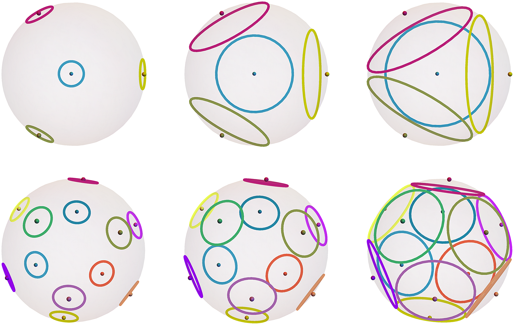
Figure 2 Circles centered at t-design points with radii increasing from left to right. The top row shows $2$
-design points and the bottom row
$2$
-design points and the bottom row $5$
-design points.
$5$
-design points.
Note that in $\mathbb {S} ^2$
the submanifold
$\mathbb {S} ^2$
the submanifold $\partial B_r(x)$
and the circle
$\partial B_r(x)$
and the circle $\Gamma _{x,r}$
coincide, so that the normalization (28) leads to
$\Gamma _{x,r}$
coincide, so that the normalization (28) leads to $\int _{\Gamma _{x,r}} f = \frac {1}{\ell (\gamma _{x,r})}\int _{\gamma _{x,r}}f$
, where
$\int _{\Gamma _{x,r}} f = \frac {1}{\ell (\gamma _{x,r})}\int _{\gamma _{x,r}}f$
, where $\gamma _{x,r}$
is the actual curve that traverses
$\gamma _{x,r}$
is the actual curve that traverses $\Gamma _{x,r}$
. In higher dimensions, this slight inconsistency between
$\Gamma _{x,r}$
. In higher dimensions, this slight inconsistency between $\Gamma _{x,r}$
and
$\Gamma _{x,r}$
and $\partial B_r(x)$
no longer occurs.
$\partial B_r(x)$
no longer occurs.
(i) According to [Reference Bondarenko, Radchenko and Viazovska3], there is a sequence $(X_t)_{t\in \mathbb {N}}$
of asymptotically optimal t-design points in
$(X_t)_{t\in \mathbb {N}}$
of asymptotically optimal t-design points in $\mathbb {S}^2$
; that is, there exist finite sets
$\mathbb {S}^2$
; that is, there exist finite sets $X_t\subset \mathbb {S}^2$
, such that
$X_t\subset \mathbb {S}^2$
, such that $|X_t|\asymp t^2$
and
$|X_t|\asymp t^2$
and
 $$ \begin{align} \frac{1}{|X_t|}\sum_{x\in X_t} f(x)=\int_{\mathbb{S}^2} f,\qquad \text{ for all } f\in \bigoplus_{k\leq t}\mathcal{H}^2_k\,. \end{align} $$
(ii) Let $r>0$
,
$r>0$
, $\Gamma ^r_t:=\bigcup _{x\in X_t}\Gamma _{x,r}$
, and
$\Gamma ^r_t:=\bigcup _{x\in X_t}\Gamma _{x,r}$
, and $\gamma ^r_t:=\dotplus _{x\in X_t}\gamma _{x,r}$
be the corresponding cycle. We first show that this cycle provides exact integration on
$\gamma ^r_t:=\dotplus _{x\in X_t}\gamma _{x,r}$
be the corresponding cycle. We first show that this cycle provides exact integration on $\Pi _t$
.
$\Pi _t$
.
For the component $\mathcal {H}^2_0=\operatorname *{\mathrm {span}}\{1\}$
, we observe
$\mathcal {H}^2_0=\operatorname *{\mathrm {span}}\{1\}$
, we observe
 $$ \begin{align*} \frac{1}{\ell(\gamma^r_t)} \int_{\gamma^r_t}1= 1=\int_{\mathbb{S}^d} 1. \end{align*} $$
We now consider $f\in \mathcal {H}^2_k$
for
$f\in \mathcal {H}^2_k$
for $1\leq k\leq t$
. Lemma 4.2 with
$1\leq k\leq t$
. Lemma 4.2 with $c_k(r):=c_{2,k}(r)$
and the definition of t-design points yields
$c_k(r):=c_{2,k}(r)$
and the definition of t-design points yields
 $$ \begin{align*} \frac{1}{\ell(\gamma^r_t)} \int_{\gamma^r_t}f & = \frac{1}{|X_t|}\sum_{x\in X_t} \frac{1}{\ell(\gamma_{x,r})} \int_{\gamma_{x,r}}f\\ & = \frac{1}{|X_t|}\sum_{x\in X_t} \int_{\Gamma_{x,r}}f\\ & = \frac{c_k(r)}{|X_t|}\sum_{x\in X_t} f(x)\\ &=c_k(r) \int_{\mathbb{S}^2} f. \end{align*} $$
Since $\mathcal {H}^2_0\perp \mathcal {H}^2_k$
for
$\mathcal {H}^2_0\perp \mathcal {H}^2_k$
for $k=1,2,\ldots $
, cf. (30), we obtain
$k=1,2,\ldots $
, cf. (30), we obtain $\int _{\mathbb {S}^2} f=0$
for
$\int _{\mathbb {S}^2} f=0$
for $f\in \mathcal {H}^2_k$
, and the factor
$f\in \mathcal {H}^2_k$
, and the factor $c_k(r)$
does not matter. We derive
$c_k(r)$
does not matter. We derive
 $$ \begin{align} \frac{1}{\ell(\gamma^r_t)} \int_{\gamma^r_t}f = \int_{\mathbb{S}^2} f \qquad \text{ for all } f\in \mathcal{H} _k^2, \end{align} $$
and, by linearity, exact quadrature holds for all $f\in \bigoplus _{k=0}^t \mathcal {H} _k^2 $
.
$f\in \bigoplus _{k=0}^t \mathcal {H} _k^2 $
.
(iii) Identity (35) holds for every $0<r<\frac {\pi }{2}$
, and thus every cycle
$0<r<\frac {\pi }{2}$
, and thus every cycle $\gamma _{t}^r$
(formal sum of closed curves) yields exact integration. We now determine radii
$\gamma _{t}^r$
(formal sum of closed curves) yields exact integration. We now determine radii $r=r_t$
depending on the degree t, so that
$r=r_t$
depending on the degree t, so that $\Gamma _t:=\Gamma ^{r_t}_t=\bigcup _{x\in X_t}\Gamma _{x,r_t}$
is indeed the trajectory of a single continuous closed curve.
$\Gamma _t:=\Gamma ^{r_t}_t=\bigcup _{x\in X_t}\Gamma _{x,r_t}$
is indeed the trajectory of a single continuous closed curve.
Let $\rho _t = \sup _{x\in \mathbb {X}}\left (\inf _{y\in X_t}\operatorname {\mathrm {dist}}_{\mathbb {X}}(x,y)\right )$
be the covering radius of
$\rho _t = \sup _{x\in \mathbb {X}}\left (\inf _{y\in X_t}\operatorname {\mathrm {dist}}_{\mathbb {X}}(x,y)\right )$
be the covering radius of $X_t$
as in (9). We choose
$X_t$
as in (9). We choose $r_t:=\rho _t$
, so that
$r_t:=\rho _t$
, so that
 $$ \begin{align} \mathbb{S}^2=\bigcup_{x\in X_t} B_{r_t}(x). \end{align} $$
The circles $\Gamma _{x,r_t}=\partial B_{r_t}(x)$
, for
$\Gamma _{x,r_t}=\partial B_{r_t}(x)$
, for $x\in X_t$
, induce a graph
$x\in X_t$
, induce a graph $\mathcal {G}$
as follows: the vertices of
$\mathcal {G}$
as follows: the vertices of $\mathcal {G} $
are the intersection points of the
$\mathcal {G} $
are the intersection points of the $\Gamma _{x,r_t}$
, and its edges are associated to arcs on these circles between the intersection points, cf. Figures 2 and 3. For each circle
$\Gamma _{x,r_t}$
, and its edges are associated to arcs on these circles between the intersection points, cf. Figures 2 and 3. For each circle $\Gamma _{x,r_t}$
, we have fixed an orientation. As a result of this construction, we obtain a directed graph
$\Gamma _{x,r_t}$
, we have fixed an orientation. As a result of this construction, we obtain a directed graph $\mathcal {G}_{\rightarrow }$
[Reference Wilson47].
$\mathcal {G}_{\rightarrow }$
[Reference Wilson47].

Figure 3 A set of connected circles induces a directed graph, whose vertices are the intersection points and whose edges are the associated arcs of the circles. Each vertex has equal in-degree and out-degree, namely, the number of circles running through this point.
Lemma 5.2. The graph $\mathcal {G}$
is strongly connected (i.e., the directed graph
$\mathcal {G}$
is strongly connected (i.e., the directed graph $\mathcal {G}_{\rightarrow }$
is connected).
$\mathcal {G}_{\rightarrow }$
is connected).
Proof. We first verify that the undirected graph $\mathcal {G}$
is connected. Pick two arbitrary but distinct vertices
$\mathcal {G}$
is connected. Pick two arbitrary but distinct vertices $v_1,v_2\in \mathcal {G}$
. Then there are points
$v_1,v_2\in \mathcal {G}$
. Then there are points $x_1,x_2\in X_t$
such that
$x_1,x_2\in X_t$
such that $v_i\in \partial B_{r_t}(x_i)$
for
$v_i\in \partial B_{r_t}(x_i)$
for $i=1,2$
. If
$i=1,2$
. If $x_1=x_2$
, then
$x_1=x_2$
, then $v_1,v_2$
are connected in
$v_1,v_2$
are connected in $\mathcal {G}$
since they lie on the same circle.
$\mathcal {G}$
since they lie on the same circle.
We may thus assume that $x_1\neq x_2$
. In this case, we consider the auxiliary graph
$x_1\neq x_2$
. In this case, we consider the auxiliary graph $\mathcal {G}_{r_t}$
treated in Lemma 4.1. Its vertices are the points of the t-design
$\mathcal {G}_{r_t}$
treated in Lemma 4.1. Its vertices are the points of the t-design $X_t$
. Two points
$X_t$
. Two points $x,y\in X_t$
are connected by an edge if and only if
$x,y\in X_t$
are connected by an edge if and only if $B_{r_t}(x)\cap B_{r_t}(y) \neq \emptyset $
. According to Lemma 4.1 and
$B_{r_t}(x)\cap B_{r_t}(y) \neq \emptyset $
. According to Lemma 4.1 and $r_t\geq \rho _t$
, the graph
$r_t\geq \rho _t$
, the graph $\mathcal {G}_{r_t}$
is connected. Thus, there is a path from
$\mathcal {G}_{r_t}$
is connected. Thus, there is a path from $x_1$
to
$x_1$
to $x_2$
in
$x_2$
in $\mathcal {G}_{r_t}$
, say
$\mathcal {G}_{r_t}$
, say $x_1=x_{i_1},\ldots ,x_{i_m}=x_2$
, so that
$x_1=x_{i_1},\ldots ,x_{i_m}=x_2$
, so that $B_{r_t}(x_{i_j})\cap B_{r_t}(x_{i_{j+1}})\neq \emptyset $
. This also implies
$B_{r_t}(x_{i_j})\cap B_{r_t}(x_{i_{j+1}})\neq \emptyset $
. This also implies $\partial B_{r_t}(x_{i_j})\cap \partial B_{r_t}(x_{i_{j+1}})\neq \emptyset $
. Clearly, vertices
$\partial B_{r_t}(x_{i_j})\cap \partial B_{r_t}(x_{i_{j+1}})\neq \emptyset $
. Clearly, vertices $v_{i_j},v_{i_{j+1}}$
of
$v_{i_j},v_{i_{j+1}}$
of $\mathcal {G}$
with
$\mathcal {G}$
with $v_{i_j}\in \partial B_{r_t}(x_{i_j})$
and
$v_{i_j}\in \partial B_{r_t}(x_{i_j})$
and $v_{i_{j+1}}\in \partial B_{r_t}(x_{i_{j+1}})$
are connected in
$v_{i_{j+1}}\in \partial B_{r_t}(x_{i_{j+1}})$
are connected in $\mathcal {G}$
. Eventually, there is a path from
$\mathcal {G}$
. Eventually, there is a path from $v_1$
to
$v_1$
to $v_2$
in
$v_2$
in $\mathcal {G}$
.
$\mathcal {G}$
.
We still need to verify that the directed graph $\mathcal {G}_{\rightarrow }$
is also connected. If two distinct vertices
$\mathcal {G}_{\rightarrow }$
is also connected. If two distinct vertices $v_{i_j},v_{i_{j+1}}$
lie on the same circle
$v_{i_j},v_{i_{j+1}}$
lie on the same circle $\partial B_{r_t}(x_1)$
, then we simply get from
$\partial B_{r_t}(x_1)$
, then we simply get from $v_{i_j}$
to
$v_{i_j}$
to $v_{i_{j+1}}$
by following the chosen orientation of
$v_{i_{j+1}}$
by following the chosen orientation of $\partial B_{r_t}(x_1)$
. No further difficulties arise, and we deduce that
$\partial B_{r_t}(x_1)$
. No further difficulties arise, and we deduce that $\mathcal {G}_{\rightarrow }$
is connected.
$\mathcal {G}_{\rightarrow }$
is connected.
By construction, each vertex of $\mathcal {G}_{\rightarrow }$
has as many incoming as outgoing edges, cf. Figure 3. Euler’s Theorem about directed, strongly connected graphs implies that there is an Euler cycle [Reference Wilson47]. Hence, all circles in
$\mathcal {G}_{\rightarrow }$
has as many incoming as outgoing edges, cf. Figure 3. Euler’s Theorem about directed, strongly connected graphs implies that there is an Euler cycle [Reference Wilson47]. Hence, all circles in $\bigcup _{x\in X_t} \partial B_{r_t}(x)=\bigcup _{x\in X_t}\Gamma _{x,r_t}$
can be traversed by a single, closed, piecewise smooth curve
$\bigcup _{x\in X_t} \partial B_{r_t}(x)=\bigcup _{x\in X_t}\Gamma _{x,r_t}$
can be traversed by a single, closed, piecewise smooth curve $\gamma _t$
on
$\gamma _t$
on $\mathbb {S}^2$
with trajectory
$\mathbb {S}^2$
with trajectory $\Gamma _t=\bigcup _{x\in X_t}\Gamma _{x,r_t}$
.
$\Gamma _t=\bigcup _{x\in X_t}\Gamma _{x,r_t}$
.
(iv) To compute the length of $\gamma _t$
, we relate the covering radius
$\gamma _t$
, we relate the covering radius $r_t $
of
$r_t $
of $X_t$
to the degree t. The same proof as in (13) shows that
$X_t$
to the degree t. The same proof as in (13) shows that $r_t \lesssim t^{-1}$
; see also [Reference Brandolini, Choirat, Colzani, Gigante, Seri and Travaglini4, Reference Breger, Ehler and Gräf6]. Therefore,
$r_t \lesssim t^{-1}$
; see also [Reference Brandolini, Choirat, Colzani, Gigante, Seri and Travaglini4, Reference Breger, Ehler and Gräf6]. Therefore, $\ell (\gamma _{x,r_t})=2\pi \sin r_t\asymp r_t \lesssim t^{-1}$
. This leads to
$\ell (\gamma _{x,r_t})=2\pi \sin r_t\asymp r_t \lesssim t^{-1}$
. This leads to
 $$ \begin{align*} \ell(\gamma_t)=|X_t| \ell(\gamma_{x,r_t})\asymp t^2 \, r_t\lesssim t. \end{align*} $$
In view of the lower bound for the length of t-design curves in Theorem 2.2, our construction yields a sequence of asymptotically optimal t-design curves.
6 General existence of spherical t-design curves
We now prove the existence of t-design curves in $\mathbb {S}^d$
for all
$\mathbb {S}^d$
for all $t\in \mathbb {N}$
in dimension
$t\in \mathbb {N}$
in dimension $d\geq 2$
. This is Theorem 1.3 of the Introduction.
$d\geq 2$
. This is Theorem 1.3 of the Introduction.
Theorem 6.1. Let $d\geq 2$
be an arbitrary integer. There is a sequence
$d\geq 2$
be an arbitrary integer. There is a sequence $(\gamma _t)_{t\in \mathbb {N}}$
of t-design curves in
$(\gamma _t)_{t\in \mathbb {N}}$
of t-design curves in $\mathbb {S}^d$
such that
$\mathbb {S}^d$
such that
 $$ \begin{align*} \ell(\gamma_t) \lesssim t^{\frac{d(d-1)}{2}}. \end{align*} $$
Furthermore, the trajectory of every $\gamma _t$
consists of a union of Euclidean circles.
$\gamma _t$
consists of a union of Euclidean circles.
We will prove this theorem by induction on the dimension d. Similar to the proof of Theorem 5.1, we first show the existence of a cycle (a formal sum of closed curves) that yields exact integration. Then we use a combinatorial argument to build a connected trajectory.
6.1 Some geometry on the sphere
Let us first state few simple observations about the action of the orthogonal group on $\mathbb {S}^d$
.
$\mathbb {S}^d$
.
Lemma 6.2. Let $d\geq 2$
and
$d\geq 2$
and $A,B\subseteq \mathbb {R}^d$
be two finite sets. If
$A,B\subseteq \mathbb {R}^d$
be two finite sets. If $0\not \in A$
, then there is a rotation
$0\not \in A$
, then there is a rotation $O\in \mathcal {O}(d)$
such that
$O\in \mathcal {O}(d)$
such that $OA\cap B=\emptyset $
.
$OA\cap B=\emptyset $
.
Proof. For the sake of completeness, we provide the simple arguments.
The claim is verified by induction. For the induction step, we identify $\mathcal {O} (d)$
as a subgroup of
$\mathcal {O} (d)$
as a subgroup of $\mathcal {O} (d+1)$
via the homomorphism
$\mathcal {O} (d+1)$
via the homomorphism $ \bar {O} \in \mathcal {O} (d) \mapsto j(\bar {O})\in \mathcal {O} (d+1)$
,
$ \bar {O} \in \mathcal {O} (d) \mapsto j(\bar {O})\in \mathcal {O} (d+1)$
, $j(\bar {O})(x) = (\bar {O}\bar {x}, x_{d+1}) $
for
$j(\bar {O})(x) = (\bar {O}\bar {x}, x_{d+1}) $
for $x = (\bar {x},x_{d+1})\in \mathbb {R} ^{d+1}$
.
$x = (\bar {x},x_{d+1})\in \mathbb {R} ^{d+1}$
.
The case $d=2$
is obvious. Consider now
$d=2$
is obvious. Consider now $A,B\subseteq \mathbb {R}^{d+1}$
. Let
$A,B\subseteq \mathbb {R}^{d+1}$
. Let $\bar {A},\bar {B}\subseteq \mathbb {R}^d$
be the orthogonal projections of
$\bar {A},\bar {B}\subseteq \mathbb {R}^d$
be the orthogonal projections of $A,B$
onto the first d coordinates.
$A,B$
onto the first d coordinates.
Case $1$
:
$1$
: $0\not \in \bar {A}$
. By the induction hypothesis, there exists
$0\not \in \bar {A}$
. By the induction hypothesis, there exists $\bar {O}\in \mathcal {O}(d)$
such that
$\bar {O}\in \mathcal {O}(d)$
such that $\bar {O}\bar {A}\cap \bar {B}=\emptyset $
. Then
$\bar {O}\bar {A}\cap \bar {B}=\emptyset $
. Then $O= j(\bar {O})\in \mathcal {O}(d+1)$
satisfies
$O= j(\bar {O})\in \mathcal {O}(d+1)$
satisfies $OA\cap B = \emptyset $
.
$OA\cap B = \emptyset $
.
Case $2$
:
$2$
: $0\in \bar {A}$
. Since
$0\in \bar {A}$
. Since $0\not \in A$
, there is
$0\not \in A$
, there is $O_1\in \mathcal {O}(d+1)$
such that
$O_1\in \mathcal {O}(d+1)$
such that $O_1A \cap (\mathbb {R} e_{d+1})=\emptyset $
. Let
$O_1A \cap (\mathbb {R} e_{d+1})=\emptyset $
. Let $A_1 = O_1A$
and
$A_1 = O_1A$
and $\bar {A_1}$
be the projection onto the first d coordinates. Then
$\bar {A_1}$
be the projection onto the first d coordinates. Then $0\not \in \overline {O_1 A}$
, and by the induction hypothesis there is
$0\not \in \overline {O_1 A}$
, and by the induction hypothesis there is $\bar {O}_2\in \mathcal {O}(d)$
such that
$\bar {O}_2\in \mathcal {O}(d)$
such that $\bar {O}_2\overline {A_1 } \cap \bar {B}=\emptyset $
. Then
$\bar {O}_2\overline {A_1 } \cap \bar {B}=\emptyset $
. Then $O = j(\bar {O}_2) O_1$
satisfies
$O = j(\bar {O}_2) O_1$
satisfies $OA \cap B = \emptyset $
.
$OA \cap B = \emptyset $
.
Corollary 6.3. Let $d\geq 2$
,
$d\geq 2$
, $v\in \mathbb {S} ^d$
and
$v\in \mathbb {S} ^d$
and $A,B\subseteq \mathbb {S}^{d}$
two finite sets. If
$A,B\subseteq \mathbb {S}^{d}$
two finite sets. If $\pm v\not \in A$
, then there is a rotation
$\pm v\not \in A$
, then there is a rotation $O\in \mathcal {O}(d+1)$
such that
$O\in \mathcal {O}(d+1)$
such that $Ov=v$
and
$Ov=v$
and $OA\cap B=\emptyset $
.
$OA\cap B=\emptyset $
.
Proof. Without loss of generality, we may assume that $v=e_{d+1}\in \mathbb {S} ^d$
. Let
$v=e_{d+1}\in \mathbb {S} ^d$
. Let $\bar {A},\bar {B}\subseteq \mathbb {R}^d$
be the orthogonal projections of
$\bar {A},\bar {B}\subseteq \mathbb {R}^d$
be the orthogonal projections of $A,B$
onto the first d coordinates. Since
$A,B$
onto the first d coordinates. Since $\pm e_{d+1}\not \in A$
, we deduce
$\pm e_{d+1}\not \in A$
, we deduce $0\not \in \bar {A}$
. According to Lemma 6.2, there is
$0\not \in \bar {A}$
. According to Lemma 6.2, there is $\bar {O}\in \mathcal {O}(d)$
such that
$\bar {O}\in \mathcal {O}(d)$
such that $\bar {O}\bar {A}\cap \bar {B}=\emptyset $
. The
$\bar {O}\bar {A}\cap \bar {B}=\emptyset $
. The $O= j(\bar {O}) \in \mathcal {O}(d+1)$
does the job.
$O= j(\bar {O}) \in \mathcal {O}(d+1)$
does the job.
As in Section 4, we now consider spherical caps and their boundary
 $$ \begin{align*} B_{r}(x)&=\{y\in\mathbb{S}^d : \operatorname{\mathrm{dist}}_{\mathbb{S}^d}(x,y)\leq r\},\\ \partial B_{r}(x) &= \{z\in\mathbb{S}^d : \|x\cos \rho_t-z\| = \sin r\}; \end{align*} $$
see (33) for $d=2$
. Clearly,
$d=2$
. Clearly, $\partial B_{r}(x)$
is homeomorphic (diffeomorphic) to the
$\partial B_{r}(x)$
is homeomorphic (diffeomorphic) to the $d-1$
-dimensional sphere
$d-1$
-dimensional sphere $\mathbb {S} ^{d-1}$
. For our analysis, we will use the following homeomorphism.
$\mathbb {S} ^{d-1}$
. For our analysis, we will use the following homeomorphism.
Let $x\in \mathbb {S}^d$
,
$x\in \mathbb {S}^d$
, $0<r<\frac {\pi }{2}$
and
$0<r<\frac {\pi }{2}$
and $O = O_x \in \mathcal {O} (d+1)$
a matrix in the orthogonal group acting on
$O = O_x \in \mathcal {O} (d+1)$
a matrix in the orthogonal group acting on $\mathbb {R}^{d+1}$
such that
$\mathbb {R}^{d+1}$
such that $x=Oe_{d+1}$
, where
$x=Oe_{d+1}$
, where $e_{d+1}=(0,\ldots ,0,1)^\top \in \mathbb {R}^{d+1}$
. Now set
$e_{d+1}=(0,\ldots ,0,1)^\top \in \mathbb {R}^{d+1}$
. Now set
 $$ \begin{align} \phi_{x,r}(z) =O\begin{pmatrix} \sin r z\\ \cos r \end{pmatrix}, \qquad z\in \mathbb{S} ^{d-1}, \end{align} $$
and recall that $e_d\in \mathbb {R}^{d}$
is the north pole in
$e_d\in \mathbb {R}^{d}$
is the north pole in $\mathbb {S}^{d-1}$
.
$\mathbb {S}^{d-1}$
.
Lemma 6.4. The map $\phi _{x,r}: \mathbb {S} ^{d-1} \to \mathbb {S} ^d$
has the following properties.
$\phi _{x,r}: \mathbb {S} ^{d-1} \to \mathbb {S} ^d$
has the following properties.
(i) $\phi _{x,r}$
is a diffeomorphism between
$\phi _{x,r}$
is a diffeomorphism between $\mathbb {S}^{d-1}$
and
$\mathbb {S}^{d-1}$
and $\partial B_r(x)$
.
$\partial B_r(x)$
.
(ii) Let $x,y\in \mathbb {S} ^{d-1}$
with
$x,y\in \mathbb {S} ^{d-1}$
with $\operatorname {\mathrm {dist}}_{\mathbb {S}^d}(x,y) < r\leq \frac {\pi }{2}$
. Then there is a unique radius
$\operatorname {\mathrm {dist}}_{\mathbb {S}^d}(x,y) < r\leq \frac {\pi }{2}$
. Then there is a unique radius $\sigma \in [\pi /3, \pi /2] $
, such that
$\sigma \in [\pi /3, \pi /2] $
, such that
 $$\begin{align*}\phi _{x,r} \big( \partial B_\sigma (e_d) \big) = \partial B_r(x) \cap \partial B_r(y) \,. \end{align*}$$
In particular, the intersection $\partial B_r(x) \cap \partial B_r(y) $
is diffeomorphic to
$\partial B_r(x) \cap \partial B_r(y) $
is diffeomorphic to $\mathbb {S} ^{d-2}$
.
$\mathbb {S} ^{d-2}$
.
Proof of Lemma 6.4.
(i) If $\|z\|=1$
, then
$\|z\|=1$
, then $\| \phi _{x,r} (z) \| ^2 = \|z\|^2 \sin ^2 r + \cos ^2 r = 1$
, and
$\| \phi _{x,r} (z) \| ^2 = \|z\|^2 \sin ^2 r + \cos ^2 r = 1$
, and
 $$ \begin{align*} \operatorname{\mathrm{dist}}(x,\phi _{x,r}(z)) &= \operatorname{\mathrm{dist}}(Oe_{d+1}, O(z \sin r, \cos r ) \\ &= \arccos \langle e_{d+1}, (z \sin r, \cos r )\rangle = r \,. \end{align*} $$
Clearly, $\phi _{x,r}$
is a bijection between
$\phi _{x,r}$
is a bijection between $\mathbb {S} ^{d-1}$
and
$\mathbb {S} ^{d-1}$
and $\partial B_r(x)$
.
$\partial B_r(x)$
.
(ii) For $z\in \mathbb {R} ^{d+1} $
, we write
$z\in \mathbb {R} ^{d+1} $
, we write $z=(z', z_{d+1}) = (z", z_d,z_{d+1})$
with
$z=(z', z_{d+1}) = (z", z_d,z_{d+1})$
with $z' \in \mathbb {R} ^d $
and
$z' \in \mathbb {R} ^d $
and $z" \in \mathbb {R} ^{d-1} $
. By applying a suitable rotation, we may assume without loss of generality that
$z" \in \mathbb {R} ^{d-1} $
. By applying a suitable rotation, we may assume without loss of generality that $x= e_{d+1}$
and
$x= e_{d+1}$
and $y = \sqrt {1-y_{d+1}^2} \, e_d + y_{d+1}e_{d+1}= (0,\sqrt {1-y_{d+1}^2},y_{d+1})$
. Then the assumption
$y = \sqrt {1-y_{d+1}^2} \, e_d + y_{d+1}e_{d+1}= (0,\sqrt {1-y_{d+1}^2},y_{d+1})$
. Then the assumption $\operatorname {\mathrm {dist}}(x,y) = \arccos \langle x,y\rangle <r$
yields
$\operatorname {\mathrm {dist}}(x,y) = \arccos \langle x,y\rangle <r$
yields $\langle x,y\rangle = y_{d+1}>\cos r$
.
$\langle x,y\rangle = y_{d+1}>\cos r$
.
Now take $z\in \partial B_{r } (e_{d+1}) \cap \partial B_{r } (y)$
. By Step (i),
$z\in \partial B_{r } (e_{d+1}) \cap \partial B_{r } (y)$
. By Step (i),
 $$\begin{align*}\partial B_r(e_{d+1}) = \phi _{e_{d+1},r}(\mathbb{S} ^{d-1}) = \{ (z' \sin r, \cos r: z' \in \mathbb{S} ^{d-1} \}, \end{align*}$$
so $z_{d+1} = \cos r $
. Since
$z_{d+1} = \cos r $
. Since $\operatorname {\mathrm {dist}} (z,y) = \arccos \langle z,y \rangle = r$
as well, we obtain
$\operatorname {\mathrm {dist}} (z,y) = \arccos \langle z,y \rangle = r$
as well, we obtain
 $$ \begin{align*} \langle z,y \rangle = z_d \sqrt{1-y_{d+1}^2} + z_{d+1} y_{d+1} = z_d \sqrt{1-y_{d+1}^2} + \cos r \,y_{d+1} = \cos r\,. \end{align*} $$
Solving for $z_d$
, this implies that
$z_d$
, this implies that
 $$ \begin{align} z_d = \cos r \, \frac{1-y_{d+1}}{\sqrt{1-y_{d+1}^2}} \,. \end{align} $$
Let us abbreviate the occurring fraction by $\tau = \frac {1-y_{d+1}}{\sqrt {1-y_{d+1}^2}}$
. Then
$\tau = \frac {1-y_{d+1}}{\sqrt {1-y_{d+1}^2}}$
. Then
 $$ \begin{align} \begin{aligned} \|z"\|^2 &= 1-z_{d+1}^2 - z_d^2\\ & = 1 - \cos ^2 r - \tau ^2 \cos ^2 r \\ &= \sin ^2 r - \tau ^2 \cos ^2 r =:s ^2 \,. \end{aligned} \end{align} $$
We may switch from $z"$
to
$z"$
to $sz"$
with
$sz"$
with $z"\in \mathbb {S}^{d-2}$
, so that every point in
$z"\in \mathbb {S}^{d-2}$
, so that every point in $z\in \partial B_r(x) \cap \partial B_r(y)$
has coordinates
$z\in \partial B_r(x) \cap \partial B_r(y)$
has coordinates
 $$ \begin{align} z= \begin{pmatrix} s z" \\ \tau \cos r \\ \cos r \end{pmatrix} \, ,\qquad z"\in \mathbb{S} ^{d-2}\,. \end{align} $$
By comparison, a point $z'\in \partial B_\sigma (e_d)\subseteq \mathbb {S} ^{d-1} $
is of the form
$z'\in \partial B_\sigma (e_d)\subseteq \mathbb {S} ^{d-1} $
is of the form $(z" \sin \sigma , \cos \sigma )$
for
$(z" \sin \sigma , \cos \sigma )$
for $z" \in \mathbb {S} ^{d-2}$
. Consequently,
$z" \in \mathbb {S} ^{d-2}$
. Consequently,
 $$ \begin{align} \phi _{e_{d+1},r}(z') = \begin{pmatrix} z" \sin \sigma \, \sin r \\ \cos \sigma \,\sin r\\ \cos r \end{pmatrix} \,. \end{align} $$
We have to show that every point in $ \partial B_{r } (x) \cap \partial B_{r } (y)$
can be represented in this way. For (40) and (41) to represent the same set, we need to verify that the following identities
$ \partial B_{r } (x) \cap \partial B_{r } (y)$
can be represented in this way. For (40) and (41) to represent the same set, we need to verify that the following identities
 $$ \begin{align} s=\sin \sigma \, \sin r \qquad \text{ and } \qquad \cos r \,\tau = \cos \sigma \, \sin r \end{align} $$
can be satisfied with a suitable choice of $\sigma $
. Clearly,
$\sigma $
. Clearly, $\sigma $
is determined by
$\sigma $
is determined by
 $$ \begin{align} \sin \sigma = \frac{s}{\sin r } \,. \end{align} $$
Then using (39),
 $$\begin{align*}\cos ^2\sigma \, \sin ^2 r = (1-\sin ^2\sigma ) \sin ^2 r = \sin ^2 r - s^2 = \tau ^2 \, \cos ^2r \, , \end{align*}$$
and the second identity in (42) is also satisfied.
Finally, since $y_{d+1} = \cos r $
and
$y_{d+1} = \cos r $
and $\tau ^2 = \frac {1-y_{d+1}}{1+y_{d+1}}$
, we estimate the size of
$\tau ^2 = \frac {1-y_{d+1}}{1+y_{d+1}}$
, we estimate the size of $\sigma $
as
$\sigma $
as
 $$ \begin{align*} \sin ^2\sigma = \frac{s^2}{\sin ^2 r} &= 1-\frac{\cos ^2 r}{\sin ^2r} \, \frac{1-y_{d+1}}{1+y_{d+1}} \\ &\geq 1-\frac{\cos ^2 r}{\sin ^2r} \, \frac{1-\cos r}{1+\cos r} \,. \end{align*} $$
For $u=\cos r\geq 0$
, we observe
$u=\cos r\geq 0$
, we observe
 $$\begin{align*}1-\frac{\cos ^2 r}{\sin ^2 r} \, \frac{1-\cos r}{1+\cos r} = 1-\frac{u^2}{1-u^2}\frac{1-u}{1+u}=1-\frac{u^2}{(1+u)^2}\geq \frac{3}{4}\,, \end{align*}$$
so that we obtain $\sin ^2\sigma \geq \frac {3}{4}$
. Consequently,
$\sin ^2\sigma \geq \frac {3}{4}$
. Consequently, $\pi /3 \leq \sigma \leq \pi /2$
, which means that
$\pi /3 \leq \sigma \leq \pi /2$
, which means that $ B_\sigma (e_d)$
covers a fixed portion of
$ B_\sigma (e_d)$
covers a fixed portion of $\mathbb {S} ^{d-1} $
.
$\mathbb {S} ^{d-1} $
.
Next, we check how curves in $\mathbb {S} ^{d-1}$
– in particular, t-design curves – are mapped by
$\mathbb {S} ^{d-1}$
– in particular, t-design curves – are mapped by $\phi _{x,r}$
.
$\phi _{x,r}$
.
Lemma 6.5. Suppose that $\gamma $
is a t-design curve in
$\gamma $
is a t-design curve in $\mathbb {S}^{d-1}$
. Let
$\mathbb {S}^{d-1}$
. Let $x\in \mathbb {S}^d$
and
$x\in \mathbb {S}^d$
and $0<r<\frac {\pi }{2}$
.
$0<r<\frac {\pi }{2}$
.
-
(i) Then
$\gamma _{x,r}=\phi _{x,r} \circ \gamma $
is a curve in
$\partial B_r(x) \subseteq \mathbb {S}^d$
with length
$\ell (\gamma _{x,r})= \ell (\gamma ) \, \sin r $
, such that
$$ \begin{align*} \frac{1}{\ell(\gamma_{x,r})}\int_{\gamma_{x,r}}f = \int_{\partial B_{r}(x)} f,\qquad \text{ for all } f\in \Pi_t \,. \end{align*} $$
-
(ii) For a given point
$w\in \partial B_r(x)$
, there is a t-design curve
$\gamma '$
in
$\mathbb {S} ^{d-1}$
, such that w lies on
$\phi _{x,r} \circ \gamma '$
. -
(iii) If
$\gamma $
consists a union of circles, then so does
$\gamma _{x,r}$
and
$\gamma '$
can also be chosen to do so. -
(iv) Assume that
$\gamma $
and
$\Psi \subseteq \mathbb {S}^d$
both consist of a finite union of circles and
$w\in \Psi $
. Then there exists a t-design curve
$\gamma "$
in
$\mathbb {S} ^{d-1} $
consisting of a union of circles, such that w is contained in the trajectory
$\Gamma ^{\prime \prime }_{x,r}$
of the curve
$\phi _{x,r} \circ \gamma "$
and the intersection
$\Gamma ^{\prime \prime }_{x,r} \cap \Psi $
is finite.


In the following, we refer to $\gamma _{x,r}$
as a t-design curve for
$\gamma _{x,r}$
as a t-design curve for $\partial B_{r}(x)$
.
$\partial B_{r}(x)$
.
Proof. (i) First we consider the north pole $x=e_{d+1}$
. The curve
$x=e_{d+1}$
. The curve $\gamma _{e_{d+1},r}= \phi _{e_{d+1},r} \circ \gamma = \left (\gamma \, \sin r , \cos r \right )^\top $
has arc length
$\gamma _{e_{d+1},r}= \phi _{e_{d+1},r} \circ \gamma = \left (\gamma \, \sin r , \cos r \right )^\top $
has arc length $\ell (\gamma _{e_{d+1},r})=\sin r \,\ell (\gamma )$
, and we derive
$\ell (\gamma _{e_{d+1},r})=\sin r \,\ell (\gamma )$
, and we derive
 $$ \begin{align*} \frac{1}{\ell(\gamma_{e_{d+1},r})}\int_{\gamma_{e_{d+1},r}}f & =\frac{1}{\sin r\, \ell(\gamma)} \int_0^1 f(\gamma (s) \, \sin r,\cos r)\|\sin r\, \dot{\gamma}(s)\| \mathrm{d}s\\ & = \frac{1}{\ell(\gamma)}\int_{\gamma}f(\;\cdot\; \sin r ,\cos r). \end{align*} $$
The last integral $\int _\gamma $
is the line integral of the function
$\int _\gamma $
is the line integral of the function $y \in \mathbb {S} ^{d-1} \mapsto f\circ \phi _{e_{d+1},r}(y) = f(y \sin r ,\cos r)$
along
$y \in \mathbb {S} ^{d-1} \mapsto f\circ \phi _{e_{d+1},r}(y) = f(y \sin r ,\cos r)$
along $\gamma $
in
$\gamma $
in $ \mathbb {S} ^{d-1}$
. For
$ \mathbb {S} ^{d-1}$
. For $f\in \Pi _t$
and
$f\in \Pi _t$
and $y\in \mathbb {S} ^{d-1}$
, the function
$y\in \mathbb {S} ^{d-1}$
, the function $f(y \sin r ,\cos r)$
is a polynomial of degree t restricted to
$f(y \sin r ,\cos r)$
is a polynomial of degree t restricted to $\mathbb {S}^{d-1}$
. The t-design property leads to
$\mathbb {S}^{d-1}$
. The t-design property leads to
 $$ \begin{align*} \frac{1}{\ell(\gamma_{e_{d+1},r})}\int_{\gamma_{e_{d+1},r}}f & = \int_{\mathbb{S}^{d-1}}f(\sin r \,\;\cdot\;,\cos r)\\ & =\int_{\partial B_{r}(e_{d+1})}f\;, \end{align*} $$
where the latter equality is due to the normalization $\int _{\mathbb {S}^{d-1}}1 = 1 = \int _{\partial B_{r}(e_{d+1})}1$
, cf. (28).
$\int _{\mathbb {S}^{d-1}}1 = 1 = \int _{\partial B_{r}(e_{d+1})}1$
, cf. (28).
For general $x\in \mathbb {S}^d$
, there is a rotation matrix O such that
$x\in \mathbb {S}^d$
, there is a rotation matrix O such that $x=Oe_{d+1}$
and rotational invariance of the distance function on
$x=Oe_{d+1}$
and rotational invariance of the distance function on $\mathbb {S} ^d$
yields
$\mathbb {S} ^d$
yields $ B_r(x)=OB_r(e_{d+1})$
and
$ B_r(x)=OB_r(e_{d+1})$
and $\partial B_{r}(x) = O\partial B_{r}(e_{d+1})$
. The curve
$\partial B_{r}(x) = O\partial B_{r}(e_{d+1})$
. The curve $\gamma _{x,r}=O\gamma _{e_{d+1},r}=\phi _{x,r} \circ \gamma $
satisfies
$\gamma _{x,r}=O\gamma _{e_{d+1},r}=\phi _{x,r} \circ \gamma $
satisfies $\|\dot {\gamma }_{x,r}\| = \|\dot {\gamma }_{e_{d+1},r}\|$
. For
$\|\dot {\gamma }_{x,r}\| = \|\dot {\gamma }_{e_{d+1},r}\|$
. For $f\in \Pi _t$
, we also have
$f\in \Pi _t$
, we also have $f\circ O\in \Pi _t$
and deduce
$f\circ O\in \Pi _t$
and deduce
 $$ \begin{align*} \int_{\partial B_{r}(x)} f = \int_{O\partial B_{r}(e_{d+1})} f & = \int_{\partial B_{r}(e_{d+1})} f\circ O\\ & = \frac{1}{\ell(\gamma_{e_{d+1},r})}\int_{\gamma_{e_{d+1},r}}f\circ O = \frac{1}{\ell(\gamma_{x,r})}\int_{\gamma_{x,r}}f. \end{align*} $$
(ii) If $\gamma $
is a t-design curve in
$\gamma $
is a t-design curve in $\mathbb {S} ^{d-1}$
, then for every orthogonal matrix
$\mathbb {S} ^{d-1}$
, then for every orthogonal matrix $U \in \mathcal {O} (d)$
the rotated curve
$U \in \mathcal {O} (d)$
the rotated curve $\gamma '=U\gamma $
is also a t-design curve in
$\gamma '=U\gamma $
is also a t-design curve in $\mathbb {S} ^{d-1}$
. By suitably choosing U, we can always achieve that a given point
$\mathbb {S} ^{d-1}$
. By suitably choosing U, we can always achieve that a given point $v\in \mathbb {S} ^{d-1}$
lies on the trajectory of
$v\in \mathbb {S} ^{d-1}$
lies on the trajectory of $U\gamma $
. Now let
$U\gamma $
. Now let $w \in \partial B_r(x)\subseteq \mathbb {S} ^d$
and
$w \in \partial B_r(x)\subseteq \mathbb {S} ^d$
and $v\in \mathbb {S} ^{d-1}$
its pre-image under
$v\in \mathbb {S} ^{d-1}$
its pre-image under $\phi _{x,r}$
. Consequently,
$\phi _{x,r}$
. Consequently, $w=\phi _{x,r}(v) $
lies on the curve
$w=\phi _{x,r}(v) $
lies on the curve $\gamma ^{\prime }_{x,r} = \phi _{x,r} \circ (U\gamma )$
.
$\gamma ^{\prime }_{x,r} = \phi _{x,r} \circ (U\gamma )$
.
(iii) Clearly, if $\gamma $
is a union of (Euclidean) circles in
$\gamma $
is a union of (Euclidean) circles in $\mathbb {S} ^{d-1}$
, then
$\mathbb {S} ^{d-1}$
, then $\gamma _{x,r}=O(\sin r\,\gamma ,\cos r)^\top $
is a union of Euclidean circles in
$\gamma _{x,r}=O(\sin r\,\gamma ,\cos r)^\top $
is a union of Euclidean circles in $\mathbb {S} ^d$
. The same holds for
$\mathbb {S} ^d$
. The same holds for $\gamma '=U\gamma $
.
$\gamma '=U\gamma $
.
(iv) Let $v = \phi _{x,r} ^{-1}(w)$
and let
$v = \phi _{x,r} ^{-1}(w)$
and let $\Psi _0 = \phi _{x,r} ^{-1} \circ (\Psi \cap \partial B_{r}(x)) $
. Then
$\Psi _0 = \phi _{x,r} ^{-1} \circ (\Psi \cap \partial B_{r}(x)) $
. Then $\Psi _0$
is again a finite union of circles or arcs of circles. Two circles are either disjoint, or they intersect in one or two points, or they coincide. This can happen only when the two circles have the same center. Let
$\Psi _0$
is again a finite union of circles or arcs of circles. Two circles are either disjoint, or they intersect in one or two points, or they coincide. This can happen only when the two circles have the same center. Let $C_\gamma \subseteq \mathbb {S} ^{d-1} $
be the set of centers of the circles of the given curve
$C_\gamma \subseteq \mathbb {S} ^{d-1} $
be the set of centers of the circles of the given curve $\gamma $
and
$\gamma $
and $C_{\Psi _0} $
be the centers of
$C_{\Psi _0} $
be the centers of $\Psi _0$
(including centers of parts of circles).
$\Psi _0$
(including centers of parts of circles).
We may assume that $\pm v\not \in C_\gamma $
(otherwise apply a rotation to
$\pm v\not \in C_\gamma $
(otherwise apply a rotation to $\gamma $
).
$\gamma $
).
Since $C_\gamma $
and
$C_\gamma $
and $C_{\Psi _0}$
are both finite and
$C_{\Psi _0}$
are both finite and $\pm v\not \in C_\gamma $
, Corollary 6.3 yields an orthogonal matrix
$\pm v\not \in C_\gamma $
, Corollary 6.3 yields an orthogonal matrix $U \in \mathcal {O} (d)$
such that
$U \in \mathcal {O} (d)$
such that $Uv=v$
and
$Uv=v$
and
 $$\begin{align*}U C_\gamma \cap C_{\Psi_0} = \emptyset \,. \end{align*}$$
The curve $\gamma " = U \gamma $
consists of circles whose centers are disjoint from those of
$\gamma " = U \gamma $
consists of circles whose centers are disjoint from those of $\Psi _0 $
; consequently,
$\Psi _0 $
; consequently, $\gamma "$
and
$\gamma "$
and $\Psi _0$
have only finitely many points in common. After mapping via
$\Psi _0$
have only finitely many points in common. After mapping via $\phi _{x,r}$
, we obtain a trajectory
$\phi _{x,r}$
, we obtain a trajectory $\Gamma ^{\prime \prime }_{x,r}=\phi _{x,r} \circ \gamma "$
in
$\Gamma ^{\prime \prime }_{x,r}=\phi _{x,r} \circ \gamma "$
in $\mathbb {S} ^d$
consisting of circles, such that
$\mathbb {S} ^d$
consisting of circles, such that $w \in \Gamma " _{x,r}$
and
$w \in \Gamma " _{x,r}$
and $\Gamma _{x,r}^{\prime \prime } \cap \Psi $
is finite.
$\Gamma _{x,r}^{\prime \prime } \cap \Psi $
is finite.
Lemma 6.6. Let $\gamma $
be a closed curve in
$\gamma $
be a closed curve in $\mathbb {S}^d$
with trajectory
$\mathbb {S}^d$
with trajectory $\Gamma $
, so that its covering radius satisfies
$\Gamma $
, so that its covering radius satisfies $r< \pi /4$
. Then
$r< \pi /4$
. Then $\Gamma $
intersects the boundary
$\Gamma $
intersects the boundary $\partial B_\sigma (x)$
for all
$\partial B_\sigma (x)$
for all $x\in \mathbb {S} ^{d-1}$
and
$x\in \mathbb {S} ^{d-1}$
and $\sigma \in ( \pi /4, \pi /2)$
:
$\sigma \in ( \pi /4, \pi /2)$
:
 $$\begin{align*}\Gamma \cap \partial B_\sigma (x) \neq \emptyset \,. \end{align*}$$
Proof. Since the covering radius of $\Gamma $
is
$\Gamma $
is $r< \pi /4$
, there exists a point
$r< \pi /4$
, there exists a point $z\in \Gamma $
, such that
$z\in \Gamma $
, such that $\operatorname {\mathrm {dist}}(z,x) \leq r$
, and thus,
$\operatorname {\mathrm {dist}}(z,x) \leq r$
, and thus, $z\in B_r(x) \subseteq B_\sigma (x)$
. Similarly, there exists a point
$z\in B_r(x) \subseteq B_\sigma (x)$
. Similarly, there exists a point $\tilde {z}\in \Gamma $
, such that
$\tilde {z}\in \Gamma $
, such that $\operatorname {\mathrm {dist}}(\tilde z,-x) \leq r$
, and thus,
$\operatorname {\mathrm {dist}}(\tilde z,-x) \leq r$
, and thus, $\tilde z\in B_r(-x) \subseteq B_\sigma (-x)$
. Since
$\tilde z\in B_r(-x) \subseteq B_\sigma (-x)$
. Since
 $$\begin{align*}\pi = \operatorname{\mathrm{dist}}(x,-x) \leq \operatorname{\mathrm{dist}}(x,\tilde{z}) + \operatorname{\mathrm{dist}}(\tilde{z},-x) \, , \end{align*}$$
we see that $\operatorname {\mathrm {dist}}(\tilde {z},x) \geq \pi - r \geq \sigma $
and
$\operatorname {\mathrm {dist}}(\tilde {z},x) \geq \pi - r \geq \sigma $
and $\tilde {z} \not \in B_\sigma (x)$
. Consequently, the continuous function
$\tilde {z} \not \in B_\sigma (x)$
. Consequently, the continuous function $\psi (s) = \operatorname {\mathrm {dist}}(\gamma (s),x) $
takes values
$\psi (s) = \operatorname {\mathrm {dist}}(\gamma (s),x) $
takes values $<\sigma $
and
$<\sigma $
and $>\sigma $
. As a consequence, there exists
$>\sigma $
. As a consequence, there exists $s_0$
, such that
$s_0$
, such that $\psi (s_0) = \operatorname {\mathrm {dist}}(\gamma (s_0),x) = \sigma $
. In other words, the point
$\psi (s_0) = \operatorname {\mathrm {dist}}(\gamma (s_0),x) = \sigma $
. In other words, the point $\gamma (s_0) $
is in
$\gamma (s_0) $
is in $\partial B_\sigma (x)$
or
$\partial B_\sigma (x)$
or $\Gamma \cap \partial B_\sigma (x)\neq \emptyset $
.
$\Gamma \cap \partial B_\sigma (x)\neq \emptyset $
.
By combining Lemma 6.5 with Lemma 4.2, we obtain that
 $$ \begin{align} \frac{1}{\ell(\gamma_{x,r})} \int _{\gamma _{x,r}} f = \int _{\partial B_r(x)} f = c_{d,k}(r) f(x) \qquad \text{ for all } f\in \mathcal{H} _k ^d \,. \end{align} $$
As in Section 5, this formula paves the way to make a transition from t-design points to t-design curves.
6.2 Part I of the proof of Theorem 6.1
Proof. We first prove the existence of a cycle (a formal sum of closed, piecewise smooth curves) in $\mathbb {S} ^d$
that yields exact integration for
$\mathbb {S} ^d$
that yields exact integration for $\Pi _t$
. We prove this claim by induction on the dimension d. The case
$\Pi _t$
. We prove this claim by induction on the dimension d. The case $d=2$
corresponds to Theorem 5.1 and shows that the optimal design curve can be realized as a union of circles. We now assume that the claim holds for
$d=2$
corresponds to Theorem 5.1 and shows that the optimal design curve can be realized as a union of circles. We now assume that the claim holds for $d-1$
with unions of circles.
$d-1$
with unions of circles.
For $0<r<\frac {\pi }{2}$
and
$0<r<\frac {\pi }{2}$
and $x\in \mathbb {S}^d$
, the induction hypothesis combined with Lemma 6.5(i) shows that there is a sequence of t-design curves
$x\in \mathbb {S}^d$
, the induction hypothesis combined with Lemma 6.5(i) shows that there is a sequence of t-design curves $\left (\gamma _{x,r,t}\right )_{t\in \mathbb {N}}$
for
$\left (\gamma _{x,r,t}\right )_{t\in \mathbb {N}}$
for $\partial B_r(x)$
of length
$\partial B_r(x)$
of length
 $$ \begin{align} \ell(\gamma_{x,r,t})\lesssim \sin r \, t^{\frac{(d-1)(d-2)}{2}} \,, \end{align} $$
whose trajectories $\Gamma _{x,r,t}=\gamma _{x,r,t}([0,1])$
consist of unions of circles.
$\Gamma _{x,r,t}=\gamma _{x,r,t}([0,1])$
consist of unions of circles.
As in the proof of Theorem 5.1, we use a sequence $(X_t)_{t\in \mathbb {N}}$
of asymptotically optimal t-design points in
$(X_t)_{t\in \mathbb {N}}$
of asymptotically optimal t-design points in $\mathbb {S}^d$
and verify that the cycle
$\mathbb {S}^d$
and verify that the cycle $\gamma _t^r = \dotplus _{x\in X_t} \gamma _{x,r,t} $
associated to the trajectory
$\gamma _t^r = \dotplus _{x\in X_t} \gamma _{x,r,t} $
associated to the trajectory $\Gamma ^r_{t}:=\bigcup _{x\in X_t} \Gamma _{x,r,t}$
provides an exact quadrature on
$\Gamma ^r_{t}:=\bigcup _{x\in X_t} \Gamma _{x,r,t}$
provides an exact quadrature on $\Pi _t$
. A careful choice of the radius r will then yield a single closed curve instead of a cycle.
$\Pi _t$
. A careful choice of the radius r will then yield a single closed curve instead of a cycle.
For the component $\mathcal {H}^2_0=\operatorname *{\mathrm {span}}\{1\}$
, we observe
$\mathcal {H}^2_0=\operatorname *{\mathrm {span}}\{1\}$
, we observe
 $$ \begin{align*} \frac{1}{\ell(\gamma^r_t)}\int_{\gamma^r_t} 1 = 1 = \int_{\mathbb{S}^d} 1. \end{align*} $$
Next, we consider $f\in \mathcal {H}^d_k$
for
$f\in \mathcal {H}^d_k$
for $1\leq k\leq t$
. On the one hand, since
$1\leq k\leq t$
. On the one hand, since $\ell (\gamma _r^t) = |X_t| \ell (\gamma _{x,r,t})$
, Lemma 6.5(i) yields
$\ell (\gamma _r^t) = |X_t| \ell (\gamma _{x,r,t})$
, Lemma 6.5(i) yields
 $$ \begin{align*} \frac{1}{\ell(\gamma^r_t)}\int_{\gamma^r_t} f & = \frac{1}{|X_t|} \sum_{x\in X_t}\frac{1}{\ell(\gamma_{x,r,t})}\int_{\gamma_{x,r,t}} f\\ & = \frac{1}{|X_t|} \sum_{x\in X_t}\int_{\partial B_{r}(x)}f. \end{align*} $$
On the other hand, by Lemma 4.2 for $f\in \mathcal {H} _k^d$
, we have
$f\in \mathcal {H} _k^d$
, we have
 $$\begin{align*}\frac{1}{|X_t|} \sum_{x\in X_t} \int_{\partial B_{r}(x)}f = c_{d,k}(r) \frac{1}{|X_t|} \sum_{x\in X_t} f(x) = c_{d,k}(r) \int _{\mathbb{S} ^d} f =0=\int _{\mathbb{S} ^d} f \,. \end{align*}$$
In combination, we obtain
 $$ \begin{align*} \frac{1}{\ell(\gamma^r_t)}\int_{\gamma^r_t} f = \int_{\mathbb{S}^d} f \end{align*} $$
for all $f\in \bigoplus _{k=0}^t \mathcal {H} _k^d$
. This concludes the first part of the proof.
$f\in \bigoplus _{k=0}^t \mathcal {H} _k^d$
. This concludes the first part of the proof.
6.3 Part II of the proof of Theorem 6.1: Existence of a single closed curve
If r is too small, then the trajectory $\Gamma ^r_t$
is not connected. If r is too big, then we may not match the desired asymptotics
$\Gamma ^r_t$
is not connected. If r is too big, then we may not match the desired asymptotics $\ell (\Gamma ^r_t)\lesssim t^{\frac {d(d-1)}{2}}$
. Since
$\ell (\Gamma ^r_t)\lesssim t^{\frac {d(d-1)}{2}}$
. Since $|X_t|\asymp t^d$
and the induction hypothesis yields
$|X_t|\asymp t^d$
and the induction hypothesis yields $ \ell (\gamma _{x,r,t})\lesssim t^{\frac {(d-1)(d-2)}{2}} \sin r $
, the total length of
$ \ell (\gamma _{x,r,t})\lesssim t^{\frac {(d-1)(d-2)}{2}} \sin r $
, the total length of $\gamma ^r_t$
is
$\gamma ^r_t$
is
 $$ \begin{align} \ell(\gamma^r_t)=\ell(\gamma_{x,r,t}) |X_t| \asymp \sin r \, t^{\frac{(d-1)(d-2)}{2}} t^d \asymp t^{\frac{d(d-1)}{2}+1} \sin r\,. \end{align} $$
This estimate suggests that we choose $r=r_t$
as
$r=r_t$
as $r_t \asymp t ^{-1}$
. Precisely, let
$r_t \asymp t ^{-1}$
. Precisely, let $\rho _t$
be the covering radius of
$\rho _t$
be the covering radius of $X_t$
; then we set
$X_t$
; then we set
 $$ \begin{align*} r_t:=2\rho_t. \end{align*} $$
Therefore, $\sin r\asymp \rho _t \lesssim t^{-1}$
, so that (46) leads to the expected total length
$\sin r\asymp \rho _t \lesssim t^{-1}$
, so that (46) leads to the expected total length
 $$ \begin{align*} \ell(\gamma^{2\rho_t}_t) \lesssim t^{-1} t^{\frac{d(d-1)}{2}+1} \asymp t^{\frac{d(d-1)}{2}}. \end{align*} $$
To ensure that $\Gamma ^{2\rho _t}_t$
is connected, we will construct
$\Gamma ^{2\rho _t}_t$
is connected, we will construct $\gamma _{x,2\rho _t,t}$
, for
$\gamma _{x,2\rho _t,t}$
, for $x\in X_t$
, in a sequential fashion.
$x\in X_t$
, in a sequential fashion.
Proof of Theorem 6.1
(Part II). As in Section 5, we consider the graph $\mathcal {G}_{\rho _t}$
with vertices
$\mathcal {G}_{\rho _t}$
with vertices $X_t$
and edges between distinct
$X_t$
and edges between distinct $x,y\in X_t$
if and only if
$x,y\in X_t$
if and only if $B_{\rho _t}(x)\cap B_{\rho _t}(y) \neq \emptyset $
. According to Lemma 4.1, the graph
$B_{\rho _t}(x)\cap B_{\rho _t}(y) \neq \emptyset $
. According to Lemma 4.1, the graph $\mathcal {G}_{\rho _t}$
is connected. Therefore, it possesses a spanning tree
$\mathcal {G}_{\rho _t}$
is connected. Therefore, it possesses a spanning tree $\mathcal {T}_{\rho _t}$
[Reference Diestel12]; this is a subgraph that contains all vertices of
$\mathcal {T}_{\rho _t}$
[Reference Diestel12]; this is a subgraph that contains all vertices of $\mathcal {G} _{\rho _t}$
such that every vertex y can be reached by a unique path from a root
$\mathcal {G} _{\rho _t}$
such that every vertex y can be reached by a unique path from a root $x_0$
.
$x_0$
.
We start at the root $x_0$
of
$x_0$
of $\mathcal {T}_{\rho _t}$
and take a t-design curve
$\mathcal {T}_{\rho _t}$
and take a t-design curve $\gamma _{x_0,2\rho _t,t}$
for
$\gamma _{x_0,2\rho _t,t}$
for $\partial B_{2\rho }(x_0)$
. Recall from Lemma 6.5 that
$\partial B_{2\rho }(x_0)$
. Recall from Lemma 6.5 that $\gamma _{x_0,2\rho _t,t}$
is obtained as the image of a t-design curve
$\gamma _{x_0,2\rho _t,t}$
is obtained as the image of a t-design curve $\gamma $
in
$\gamma $
in $\mathbb {S} ^{d-1}$
via the diffeomorphism
$\mathbb {S} ^{d-1}$
via the diffeomorphism $\phi _{x_0,2\rho _t}$
as
$\phi _{x_0,2\rho _t}$
as $\gamma _{x_0,2\rho _t,t} = \phi _{x_0,2\rho _t} (\gamma )$
and we suppose that the trajectory of
$\gamma _{x_0,2\rho _t,t} = \phi _{x_0,2\rho _t} (\gamma )$
and we suppose that the trajectory of $\gamma $
is a union of circles.
$\gamma $
is a union of circles.
Now consider the first descendant $x_1$
of
$x_1$
of $x_0$
in the tree
$x_0$
in the tree $\mathcal {T}_{\rho _t}$
. Since
$\mathcal {T}_{\rho _t}$
. Since $\operatorname {\mathrm {dist}}(x_0,x_1)\leq 2\rho _t$
, Lemma 6.4(ii) (with
$\operatorname {\mathrm {dist}}(x_0,x_1)\leq 2\rho _t$
, Lemma 6.4(ii) (with $r=2\rho _t$
) implies that
$r=2\rho _t$
) implies that
 $$\begin{align*}\partial B_{2\rho _{t}}(x_0) \cap \partial B_{2\rho _t}(x_1) = \phi _{x_0,2\rho _t} \big( \partial B_\sigma (e_d) \big) \end{align*}$$
for some $\sigma> \pi / 4$
. Since
$\sigma> \pi / 4$
. Since $\gamma $
is a t-design curve in
$\gamma $
is a t-design curve in $\mathbb {S} ^{d-1}$
, the covering radius of its trajectory is of the order
$\mathbb {S} ^{d-1}$
, the covering radius of its trajectory is of the order $t ^{-1} $
and is thus smaller than
$t ^{-1} $
and is thus smaller than $\sigma $
for t large enough. Lemma 6.6 implies that
$\sigma $
for t large enough. Lemma 6.6 implies that $\Gamma \cap \partial B_\sigma (e_d) \neq \emptyset $
, and after applying
$\Gamma \cap \partial B_\sigma (e_d) \neq \emptyset $
, and after applying $\phi _{x_0, 2\rho _t}$
we obtain that
$\phi _{x_0, 2\rho _t}$
we obtain that
 $$\begin{align*}\Gamma _{x_0,2\rho_t,t} \cap \partial B_{2\rho _{t}}(x_0) \cap \partial B_{2\rho _t}(x_1) \neq \emptyset \,. \end{align*}$$
Let $w_1\in \mathbb {S} ^d$
be a point in this intersection. By Lemma 6.5(iv) applied to
$w_1\in \mathbb {S} ^d$
be a point in this intersection. By Lemma 6.5(iv) applied to $\Psi = \Gamma _{x_0,2\rho _t,t}$
and
$\Psi = \Gamma _{x_0,2\rho _t,t}$
and $w_1$
, there exists a t-design curve
$w_1$
, there exists a t-design curve $\tilde \gamma $
in
$\tilde \gamma $
in $\mathbb {S} ^{d-1} $
, whose image
$\mathbb {S} ^{d-1} $
, whose image $\phi _{x_1,2\rho _t} (\tilde {\gamma }) = \gamma _{x_1,2\rho _t,t}$
is a t-design for
$\phi _{x_1,2\rho _t} (\tilde {\gamma }) = \gamma _{x_1,2\rho _t,t}$
is a t-design for $\partial B_{2\rho }(x_1)$
such that
$\partial B_{2\rho }(x_1)$
such that $w_1\in \Gamma _{x_1,2\rho _t,t}$
and the intersection
$w_1\in \Gamma _{x_1,2\rho _t,t}$
and the intersection $\Gamma _{x_0,2\rho _t,t}\cap \Gamma _{x_1,2\rho _t,t}$
contains only finitely many points.
$\Gamma _{x_0,2\rho _t,t}\cap \Gamma _{x_1,2\rho _t,t}$
contains only finitely many points.
The next descendant $x_2$
leads to
$x_2$
leads to
 $$\begin{align*}\partial B_{2\rho _{t}}(x_1) \cap \partial B_{2\rho _t}(x_2) = \phi _{x_1,2\rho _t} \big( \partial B_\sigma (e_d) \big) \end{align*}$$
for some $\sigma> \pi / 4$
. The same arguments as above yield the existence of
$\sigma> \pi / 4$
. The same arguments as above yield the existence of
 $$\begin{align*}w_2\in \Gamma _{x_1,2\rho_t,t} \cap \partial B_{2\rho _{t}}(x_1) \cap \partial B_{2\rho _t}(x_2)\,. \end{align*}$$
We now apply Lemma 6.5(iv) with $w_2$
and
$w_2$
and $\Psi = \Gamma _{x_0,2\rho _t,t} \cup \Gamma _{x_1,2\rho _t,t}$
and obtain a t-design curve
$\Psi = \Gamma _{x_0,2\rho _t,t} \cup \Gamma _{x_1,2\rho _t,t}$
and obtain a t-design curve $\Gamma _{x_2,2\rho _t,t}$
in
$\Gamma _{x_2,2\rho _t,t}$
in $\partial B_{\rho _t}(x_2)$
, such that
$\partial B_{\rho _t}(x_2)$
, such that $w_2\in \Gamma _{x_2,2\rho _t,t}$
and
$w_2\in \Gamma _{x_2,2\rho _t,t}$
and $\Gamma _{x_2,2\rho _t,t} \cap \big (\Gamma _{x_0,2\rho _t,t}\cup \Gamma _{x_1,2\rho _t,t}\big )$
is finite.
$\Gamma _{x_2,2\rho _t,t} \cap \big (\Gamma _{x_0,2\rho _t,t}\cup \Gamma _{x_1,2\rho _t,t}\big )$
is finite.
This process is repeated until we reach a leaf of the spanning tree $\mathcal {T}_{\rho _t}$
. Then we return to the last branch-off in
$\mathcal {T}_{\rho _t}$
. Then we return to the last branch-off in $\mathcal {T}_{\rho _t}$
and proceed with the next branch of the tree.
$\mathcal {T}_{\rho _t}$
and proceed with the next branch of the tree.
Finally, this construction leads to a connected set of circles in $\mathbb {S} ^d$
, and the resulting trajectory
$\mathbb {S} ^d$
, and the resulting trajectory $\Gamma _t:=\bigcup _{x\in X_t}\Gamma _{x,2\rho _t,t}$
of all curves is a connected set with finitely many intersection points.
$\Gamma _t:=\bigcup _{x\in X_t}\Gamma _{x,2\rho _t,t}$
of all curves is a connected set with finitely many intersection points.
By construction, $\Gamma _t$
is a connected set of finitely many circles. Although Lemma 5.2 is formulated for a graph
$\Gamma _t$
is a connected set of finitely many circles. Although Lemma 5.2 is formulated for a graph $\mathcal {G}$
constructed from finitely many circles in
$\mathcal {G}$
constructed from finitely many circles in $\mathbb {S}^2$
, its proof only uses combinatorial arguments and hence also holds for circles in
$\mathbb {S}^2$
, its proof only uses combinatorial arguments and hence also holds for circles in $\mathbb {S}^d$
. Since
$\mathbb {S}^d$
. Since $\Gamma _t$
is connected, so is
$\Gamma _t$
is connected, so is $\mathcal {G}$
. The second part of the proof of Lemma 5.2 shows that we may fix an arbitrary orientation, and then the corresponding directed graph
$\mathcal {G}$
. The second part of the proof of Lemma 5.2 shows that we may fix an arbitrary orientation, and then the corresponding directed graph $\mathcal {G}_{\rightarrow }$
is also connected. Thus,
$\mathcal {G}_{\rightarrow }$
is also connected. Thus, $\Gamma _t$
can be traversed by a single continuous curve. See again Figure 3 for a pictorial argument.
$\Gamma _t$
can be traversed by a single continuous curve. See again Figure 3 for a pictorial argument.
7 Some applications
We now discuss a few direct applications of t-design curves to mobile sampling on the sphere and exact integration of polynomials with respect to the measure $\mathrm {e}^{-\|x\|}\mathrm {d}x$
on
$\mathrm {e}^{-\|x\|}\mathrm {d}x$
on $\mathbb {R}^d$
.
$\mathbb {R}^d$
.
7.1 Mobile sampling on the sphere
Here we prove Corollary 1.4 of the Introduction and show that a polynomial f of degree t can be reconstructed from its restriction to a $2t$
-design curve.
$2t$
-design curve.
For its formulation, we recall that $\Pi _t$
restricted to
$\Pi _t$
restricted to $\mathbb {S}^d$
is a reproducing kernel Hilbert space with respect to the inner product from
$\mathbb {S}^d$
is a reproducing kernel Hilbert space with respect to the inner product from $L^2(\mathbb {S} ^d)$
. This means that for every
$L^2(\mathbb {S} ^d)$
. This means that for every $x\in \mathbb {S} ^d$
, there is a polynomial
$x\in \mathbb {S} ^d$
, there is a polynomial $k_x \in \Pi _t$
, such that
$k_x \in \Pi _t$
, such that
 $$\begin{align*}f(x) = \langle f, k_x \rangle = \int _{\mathbb{S} ^d} f \, \overline{k_x} \,. \end{align*}$$
This kernel possesses an explicit description by means of zonal spherical harmonics and Gegenbauer (or ultraspherical) polynomials [Reference Stein and Weiss43]. Let $P^\lambda _k, k\in \mathbb {N},$
be the sequence of Gegenbauer polynomials associated with
$P^\lambda _k, k\in \mathbb {N},$
be the sequence of Gegenbauer polynomials associated with $\lambda>0$
. They are defined by their generating function
$\lambda>0$
. They are defined by their generating function
 $$\begin{align*}(1-2rx + r^2)^{-\lambda } = \sum _{k=0}^\infty P^\lambda _k(x) r^k \,. \end{align*}$$
Using [43, Thm. 2.14], there are real constants $b_{k,d}$
, such that
$b_{k,d}$
, such that
 $$ \begin{align} k_x (y) = \sum _{k=0}^t b_{k,d} P^{\frac{d-1}{2}}_k(x\cdot y) \, \qquad x,y \in \mathbb{S} ^d \,. \end{align} $$
We can now extend the formulation of Corollary 1.4 of the Introduction as follows.
Proposition 7.1. Let $\gamma $
be a
$\gamma $
be a $2t$
-design curve on
$2t$
-design curve on $\mathbb {S} ^d$
and f a restriction of a polynomial of degree t onto
$\mathbb {S} ^d$
and f a restriction of a polynomial of degree t onto $\mathbb {S}^d$
. Then
$\mathbb {S}^d$
. Then
 $$ \begin{align} \frac{1}{\ell (\gamma )} \int _\gamma |f|^2 = \int _{\mathbb{S} ^d} |f|^2, \, \end{align} $$
and f is reconstructed from its values along $\gamma $
by
$\gamma $
by
 $$ \begin{align} f(x)= \frac{1}{\ell (\gamma ) } \int _{\gamma} f k_x ,\quad\text{for all } x\in\mathbb{S}^d\,. \end{align} $$
Proof. We only need to prove the reconstruction formula (49). Since $f k_x\in \Pi _{2t}$
and
$f k_x\in \Pi _{2t}$
and $k_x$
is real-valued, the reproducing property yields
$k_x$
is real-valued, the reproducing property yields
 $$ \begin{align*} f(x) = \int _{\mathbb{S} ^d} f \, k_x = \frac{1}{\ell (\gamma ) } \int _{\gamma} f k_x\,.\\[-45pt] \end{align*} $$
7.2 Integration of polynomials on
$\mathbb {R}^d$
with respect to
$\mathrm {e}^{-\|x\|}\mathrm {d}x$


Next we consider the integration problem
 $$ \begin{align*} \int_{\mathbb{R}^d} f(x)\mathrm{e}^{-\|x\|}\mathrm{d}x. \end{align*} $$
Recall that the family of generalized Laguerre polynomials $(L^{(d-1)}_n)_{n\in \mathbb {N}}$
are orthogonal with respect to the measure
$(L^{(d-1)}_n)_{n\in \mathbb {N}}$
are orthogonal with respect to the measure $r^{d-1}\mathrm {e}^{-r}\mathrm {d}r$
on
$r^{d-1}\mathrm {e}^{-r}\mathrm {d}r$
on $[0,\infty )$
. Using the zeros of
$[0,\infty )$
. Using the zeros of $L_n^{(d-1)}$
, we obtain the following quadrature rule, where
$L_n^{(d-1)}$
, we obtain the following quadrature rule, where $\Pi _t$
now stands for polynomials of degree at most t in d variables.
$\Pi _t$
now stands for polynomials of degree at most t in d variables.
Corollary 7.2. Let $\gamma $
be a spherical t-design curve in
$\gamma $
be a spherical t-design curve in $\mathbb {S}^{d-1}$
. For every integer
$\mathbb {S}^{d-1}$
. For every integer $n\geq \frac {t+1}{2}$
, let
$n\geq \frac {t+1}{2}$
, let $\{r_j\}_{j=1}^n\subset (0,\infty )$
be the set of zeros of
$\{r_j\}_{j=1}^n\subset (0,\infty )$
be the set of zeros of $L^{(d-1)}_n$
with the associated weights
$L^{(d-1)}_n$
with the associated weights $\{w_j\}_{j=1}^n\subset (0,\infty )$
for Gaussian quadrature. Then we have
$\{w_j\}_{j=1}^n\subset (0,\infty )$
for Gaussian quadrature. Then we have
 $$ \begin{align*} \int_{\mathbb{R}^d} f(x)\mathrm{e}^{-\|x\|}\mathrm{d}x = \frac{\operatorname*{\mathrm{vol}}(\mathbb{S}^{d-1})}{\ell(\gamma)}\sum_{j=1}^{n} \frac{w_j}{r_j} \int_{r_j\gamma} f, \qquad \text{ for all } f\in\Pi_t. \end{align*} $$
Thus, the scaled curves $\{r_j\gamma \}_{j=1}^{n}$
with weights
$\{r_j\gamma \}_{j=1}^{n}$
with weights $\{\frac {w_j\operatorname *{\mathrm {vol}}(\mathbb {S}^{d-1})}{r_j \ell (\gamma )}\}_{j=1}^{n}$
form an exact quadrature rule for
$\{\frac {w_j\operatorname *{\mathrm {vol}}(\mathbb {S}^{d-1})}{r_j \ell (\gamma )}\}_{j=1}^{n}$
form an exact quadrature rule for $\Pi _t$
with respect to the measure
$\Pi _t$
with respect to the measure $\mathrm {e}^{-\|x\|}\mathrm {d}x$
.
$\mathrm {e}^{-\|x\|}\mathrm {d}x$
.
Proof. Gaussian quadrature based on the zeros of $L_n^{(d-1)}$
is exact for all univariate polynomials g of degree at most
$L_n^{(d-1)}$
is exact for all univariate polynomials g of degree at most $t\leq 2n-1$
; that is,
$t\leq 2n-1$
; that is,
 $$ \begin{align*} \int_0^\infty g(r)r^{d-1}\mathrm{e}^{-r}\mathrm{d}r = \sum_{j=1}^{n} w_j g(r_j). \end{align*} $$
Let $f\in \Pi _t$
. For fixed
$f\in \Pi _t$
. For fixed $z\in \mathbb {S} ^{d-1}$
, the function
$z\in \mathbb {S} ^{d-1}$
, the function $r\mapsto f(rz)$
is a univariate polynomial of degree at most t, and therefore,
$r\mapsto f(rz)$
is a univariate polynomial of degree at most t, and therefore,
 $$ \begin{align*} \int_{\mathbb{R}^d} f(x)\mathrm{e}^{-\|x\|}\mathrm{d}x & = \int_{\mathbb{S}^{d-1}} \int_0^\infty f(rz)r^{d-1}\mathrm{e}^{-r}\mathrm{d}r \mathrm{d}z\\ & = \int_{\mathbb{S}^{d-1}} \Big(\sum_{j=1}^{n} w_j f(r_j z ) \Big) \mathrm{d}z. \end{align*} $$
Since $\gamma $
is a t-design curve on
$\gamma $
is a t-design curve on $\mathbb {S} ^{d-1}$
and
$\mathbb {S} ^{d-1}$
and $z\mapsto f(r_jz)$
is a polynomial in
$z\mapsto f(r_jz)$
is a polynomial in $\Pi _t$
, we derive
$\Pi _t$
, we derive
 $$ \begin{align*} \int_{\mathbb{R}^d} f(x)\mathrm{e}^{-\|x\|}\mathrm{d}x & = \frac{\operatorname*{\mathrm{vol}}(\mathbb{S}^{d-1})}{\ell(\gamma)}\int_\gamma \sum_{j=1}^{n} w_j f(r_j\cdot)\\ & = \frac{\operatorname*{\mathrm{vol}}(\mathbb{S}^{d-1})}{\ell(\gamma)}\sum_{j=1}^{n} w_j \int_0^1 f(r_j\gamma(s))\|\dot{\gamma}(s)\|\mathrm{d}s\\ & = \frac{\operatorname*{\mathrm{vol}}(\mathbb{S}^{d-1})}{\ell(\gamma)} \sum_{j=1}^{n} \frac{w_j}{r_j} \int_0^1 f(r_j\gamma(s))\|r_j\dot{\gamma}(s)\|\mathrm{d}s\\ & = \frac{\operatorname*{\mathrm{vol}}(\mathbb{S}^{d-1})}{\ell(\gamma)}\sum_{j=1}^{n} \frac{w_j}{r_j} \int_{r_j\gamma} f.\\[-48pt] \end{align*} $$
Example 7.3. Let $\gamma ^{(3,a_3)}$
be the spherical
$\gamma ^{(3,a_3)}$
be the spherical $3$
-design curve of Proposition 3.1. The zeros of
$3$
-design curve of Proposition 3.1. The zeros of $L^{(2)}_2(r) = \tfrac {1}{2} r^2 -4r+6$
are
$L^{(2)}_2(r) = \tfrac {1}{2} r^2 -4r+6$
are $r_1=2$
and
$r_1=2$
and $r_2=6$
. The associated Gaussian weights are
$r_2=6$
. The associated Gaussian weights are $w_1=\frac {3}{2}$
and
$w_1=\frac {3}{2}$
and $w_2=\frac {1}{2}$
. Therefore, we obtain
$w_2=\frac {1}{2}$
. Therefore, we obtain
 $$ \begin{align} \int_{\mathbb{R}^3} f(x)\mathrm{e}^{-\|x\|}\mathrm{d}x = \frac{3\pi}{\ell(\gamma^{(3,a_3)})}\int_{2\gamma^{(3,a_3)}} f + \frac{\pi}{3\ell(\gamma^{(3,a_3)})}\int_{6\gamma^{(3,a_3)}} f, \end{align} $$
for $f\in \Pi _3$
; see (a) in Figure 4.
$f\in \Pi _3$
; see (a) in Figure 4.
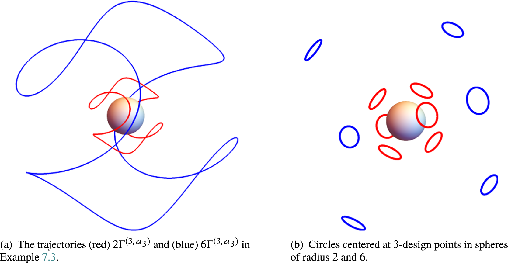
Figure 4 Trajectories provide exact integration of all polynomials in three variables of degree at most $3$
with respect to the measure
$3$
with respect to the measure $\mathrm {e}^{-\|x\|}\mathrm {d}x$
. The unit sphere in the center is shown as a reference.
$\mathrm {e}^{-\|x\|}\mathrm {d}x$
. The unit sphere in the center is shown as a reference.
Example 7.4. Consider t-design points $X_t\subset \mathbb {S}^{2}$
and take curves
$X_t\subset \mathbb {S}^{2}$
and take curves $\gamma _{x,r}$
whose trajectory are Euclidean circles
$\gamma _{x,r}$
whose trajectory are Euclidean circles $\Gamma _{x,r}$
of radius
$\Gamma _{x,r}$
of radius $\sin r$
centered at
$\sin r$
centered at $x\in X_t$
as in the proof of Theorem 5.1. Analogous to Corollary 7.2, we may scale via the zeros of
$x\in X_t$
as in the proof of Theorem 5.1. Analogous to Corollary 7.2, we may scale via the zeros of $L^{(d-1)}_n$
and use the associated Gaussian quadrature weights to obtain
$L^{(d-1)}_n$
and use the associated Gaussian quadrature weights to obtain
 $$ \begin{align*} \int_{\mathbb{R}^3} f(x)\mathrm{e}^{-\|x\|}\mathrm{d}x=\frac{2}{\sin r |X_t|}\sum_{j=1}^n \sum_{x\in X_t} \frac{w_j}{r_j }\int_{r_j\gamma_{x,r}} f,\qquad f\in\Pi_t; \end{align*} $$
see (b) in Figure 4 for $t=3$
.
$t=3$
.
Funding statement
K. G. was supported in part by the project P31887-N32 of the Austrian Science Fund (FWF).
Competing interest
The authors have no competing interest to declare.


 Open access