


Determinantal point processes (DPPs) are processes that capture negative correlations. The more similar two points are, the less likely they are to be sampled simultaneously. Then DPPs tend to create sets of diverse points. They naturally arise in random matrix theory [Reference Ginibre22] or in the modeling of a natural repulsive phenomenon such as the repartition of trees in a forest [Reference Lavancier, Møller and Rubak31]. Ever since the work of Kulesza and Taskar [Reference Kulesza and Taskar27], these processes have become more and more popular in machine learning, because of their ability to draw subsamples that account for the inner diversity of data sets. This property is useful for many applications, such as summarizing documents [Reference Dupuy and Bach14], improving a stochastic gradient descent by drawing diverse subsamples at each step [Reference Zhang, Kjellström and Mandt45], or extracting a meaningful subset of a large data set to estimate a cost function or some parameters [Reference Amblard, Barthelmé and Tremblay3, Reference Bardenet, Lavancier, Mary and Vasseur6, Reference Tremblay, Barthelmé and Amblard44]. Several issues are under investigation, such as learning DPPs, for instance through maximum likelihood estimation [Reference Brunel, Moitra, Rigollet and Urschel10, Reference Kulesza and Taskar28], or sampling these processes. Here we will focus on the sampling question and we will only deal with a discrete and finite determinantal point process Y, defined by its kernel matrix K, a configuration particularly adapted to machine learning data sets.
The main algorithm to sample DPPs is a spectral algorithm [Reference Hough, Krishnapur, Peres and Virág24]: it uses the eigendecomposition of K to sample Y. It is exact and in general quite fast. However, the computation of the eigenvalues of K may be very costly when dealing with large-scale data. That is why numerous algorithms have been conceived to bypass this issue. Some authors have tried to design a sampling algorithm adapted to specific DPPs. For instance, it is possible to speed up the initial algorithm by assuming that K has a bounded rank: see Gartrell, Paquet, and Koenigstein [Reference Gartrell, Paquet and Koenigstein15] and Kulesza and Taskar [Reference Kulesza and Taskar26]. They used a dual representation of the kernel so that almost all the computations in the spectral algorithm are reduced. One can also deal with another class of DPPs associated with kernels K that can be decomposed into a sum of tractable matrices: see Dupuy and Bach [Reference Dupuy and Bach14]. In this case the sampling is much faster, and Dupuy and Bach studied inference on these classes of DPPs. Finally, Propp and Wilson [Reference Propp and Wilson37] used Markov chains and the theory of coupling from the past to sample exactly particular DPPs: uniform spanning trees. Adapting Wilson’s algorithm, Avena and Gaudillière [Reference Avena and Gaudillière5] provided another algorithm to efficiently sample a parametrized DPP kernel associated with random spanning forests.
Another type of sampling algorithms is the class of approximate methods. Some authors have approached the original DPP with a low-rank matrix, either by random projections [Reference Gillenwater, Kulesza and Taskar21, Reference Kulesza and Taskar27] or using the Nyström approximation [Reference Affandi, Kulesza, Fox and Taskar1]. The Monte Carlo Markov chain methods also offer nice approximate sampling algorithms for DPPs. It is possible to obtain satisfying convergence guarantees for particular DPPs, for instance k-DPPs with fixed cardinality [Reference Anari, Gharan and Rezaei4, Reference Li, Jegelka and Sra32] or projection DPPs [Reference Gautier, Bardenet and Valko17]. Li, Sra, and Jegelka [Reference Li, Sra and Jegelka33] even proposed a polynomial-time sampling algorithm for general DPPs, thus correcting the initial work of Kang [Reference Kang25]. These algorithms are commonly used as they save significant time, but the price to pay is the lack of precision of the result.
As one can see, except for the initial spectral algorithm, no algorithm allows for the exact sampling of a general DPP. The main contribution of this paper is to introduce such a general and exact algorithm that does not involve the kernel eigendecomposition, to sample discrete DPPs. The proposed algorithm is a sequential thinning procedure that relies on two new results: (i) the explicit formulation of the marginals of any determinantal point process, and (ii) the derivation of an adapted Bernoulli point process containing a given DPP. This algorithm was first presented in [Reference Launay, Galerne and Desolneux29] and was, to our knowledge, the first exact sampling strategy without spectral decomposition. MATLAB® and Python implementations of this algorithm (using the PyTorch library in the Python code) are available online (https://www.math-info.univ-paris5.fr/~claunay/exact_sampling.html) and hopefully soon in the repository created by Guillaume Gautier [Reference Gautier, Polito, Bardenet and Valko18] gathering exact and approximate DPP sampling algorithms. Let us mention that three very recent papers, [Reference Poulson36], [Reference Gillenwater, Kulesza, Mariet and Vassilvtiskii20], and [Reference Dereziński, Calandriello and Valko13], also propose new algorithms to sample general DPPs without spectral decomposition. Poulson [Reference Poulson36] presents factorization strategies of Hermitian and non-Hermitian DPP kernels to sample general determinantal point processes. Like our algorithm, it relies heavily on Cholesky decomposition. Gillenwater et al. [Reference Gillenwater, Kulesza, Mariet and Vassilvtiskii20] use the dual representation of L-ensembles presented in [Reference Kulesza and Taskar27] to construct a binary tree containing enough information on the kernel to sample DPPs in sublinear time. Dereziński, Calandriello, and Valko [Reference Dereziński, Calandriello and Valko13] apply a preprocessing step that preselects a portion of the points using a regularized DPP. Then a typical DPP sampling is done on the selection. This is related to our thinning procedure of the initial set by a Bernoulli point process. However, note that Dereziński et al. report that the overall complexity of their sampling scheme is sublinear, while ours is cubic due to Cholesky decomposition. Finally, Błaszczyszyn and Keeler [Reference Błaszczyszyn and Keeler8] present a similar procedure based on a continuous space: they use discrete determinantal point processes to thin a Poisson point process defined on that continuous space. The point process generated offers theoretical guarantees on repulsion and is used to fit network patterns.
The rest of the paper is organized as follows. In the next section we present the general framework of determinantal point processes and the classic spectral algorithm. In Section 2 we provide an explicit formulation of the general marginals and pointwise conditional probabilities of any determinantal point process, from its kernel K. Using these formulations, we first introduce a ‘naive’, exact but slow, sequential algorithm that relies on the Cholesky decomposition of the kernel K. In Section 3, using the thinning theory, we accelerate the previous algorithm and introduce a new exact sampling algorithm for DPPs that we call the sequential thinning algorithm. Its computational complexity is compared with that of the two previous algorithms. In Section 4 we display the results of some experiments comparing these three sampling algorithms, and we describe the conditions under which the sequential thinning algorithm is more efficient than the spectral algorithm. Finally, we discuss and conclude on this algorithm.
1. DPPs and their usual sampling method: the spectral algorithm
In the next sections we will use the following notation. Let us consider a discrete finite set $\mathcal{Y} = \{1, \dots, N\}$
. This set represents the space on which the point process is defined. In point process theory, it can be called the carrier space or state space. In this paper we choose a machine learning term and refer to
$\mathcal{Y} = \{1, \dots, N\}$
. This set represents the space on which the point process is defined. In point process theory, it can be called the carrier space or state space. In this paper we choose a machine learning term and refer to ${\mathcal{Y}}$
as the ground set. For
${\mathcal{Y}}$
as the ground set. For $M \in {\mathbb{R}}^{N\times N}$
a matrix, we will denote by
$M \in {\mathbb{R}}^{N\times N}$
a matrix, we will denote by $M_{A \times B}$
, for all
$M_{A \times B}$
, for all $ A,B \subset {\mathcal{Y}}$
, the matrix
$ A,B \subset {\mathcal{Y}}$
, the matrix $(M(i,j))_{(i,j) \in A \times B}$
and the short notation
$(M(i,j))_{(i,j) \in A \times B}$
and the short notation $M_A = M_{A \times A}$
. Suppose that K is a Hermitian positive semi-definite matrix of size
$M_A = M_{A \times A}$
. Suppose that K is a Hermitian positive semi-definite matrix of size $N \times N$
, indexed by the elements of
$N \times N$
, indexed by the elements of $\mathcal{Y}$
, so that any of its eigenvalues is in [0, 1]. A subset
$\mathcal{Y}$
, so that any of its eigenvalues is in [0, 1]. A subset $Y \subset \mathcal{Y}$
is said to follow a DPP distribution of kernel K if
$Y \subset \mathcal{Y}$
is said to follow a DPP distribution of kernel K if
 \begin{equation*}\mathbb{P}( A \subset Y ) = \det(K_A) \quad\text{{for all} } A \subset \mathcal{Y}.\end{equation*}
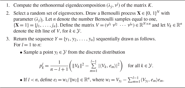
The spectral algorithm is standard for drawing a determinantal point process. It relies on the eigendecomposition of its kernel K. It was first introduced by Hough et al. [Reference Hough, Krishnapur, Peres and Virág24] and is also presented in a more detailed way by Scardicchio [Reference Scardicchio, Zachary and Torquato40], Kulesza and Taskar [Reference Kulesza and Taskar27], or Lavancier, Møller, and Rubak [Reference Lavancier, Møller and Rubak31]. It proceeds in three steps. The first step is the computation of the eigenvalues $\lambda_j$
and the eigenvectors
$\lambda_j$
and the eigenvectors $v^j$
of the matrix K. The second step consists in randomly selecting a set of eigenvectors according to N Bernoulli variables of parameter
$v^j$
of the matrix K. The second step consists in randomly selecting a set of eigenvectors according to N Bernoulli variables of parameter $\lambda_i$
, for
$\lambda_i$
, for $i=1,\dots,N$
. The third step is drawing sequentially the associated points using a Gram–Schmidt process.
$i=1,\dots,N$
. The third step is drawing sequentially the associated points using a Gram–Schmidt process.
Algorithm 1 The spectral sampling algorithm
This algorithm is exact and relatively fast, but it becomes slow when the size of the ground set grows. For a ground set of size N and a sample of size n, the third step costs ${\text{O}}(Nn^3)$
because of the Gram–Schmidt orthonormalization. Tremblay, Barthelmé, and Amblard [Reference Tremblay, Barthelmé and Amblard43] proposed speeding it up using optimized computations and they achieved the complexity
${\text{O}}(Nn^3)$
because of the Gram–Schmidt orthonormalization. Tremblay, Barthelmé, and Amblard [Reference Tremblay, Barthelmé and Amblard43] proposed speeding it up using optimized computations and they achieved the complexity ${\text{O}}(Nn^2)$
for this third step. Nevertheless, the eigendecomposition of the matrix K is the heaviest part of the algorithm, as it runs in time
${\text{O}}(Nn^2)$
for this third step. Nevertheless, the eigendecomposition of the matrix K is the heaviest part of the algorithm, as it runs in time ${\text{O}}(N^3)$
, and we will see in the numerical results that this first step generally comprises more than 90% of the running time of the spectral algorithm. As the amount of data continues to explode, in practice the matrix K is very large, so it seems relevant to try to avoid this costly operation. We compare the time complexities of the different algorithms presented in this paper at the end of Section 3. In the next section we show that any DPP can be exactly sampled by a sequential algorithm that does not require the eigendecomposition of K.
${\text{O}}(N^3)$
, and we will see in the numerical results that this first step generally comprises more than 90% of the running time of the spectral algorithm. As the amount of data continues to explode, in practice the matrix K is very large, so it seems relevant to try to avoid this costly operation. We compare the time complexities of the different algorithms presented in this paper at the end of Section 3. In the next section we show that any DPP can be exactly sampled by a sequential algorithm that does not require the eigendecomposition of K.
2. Sequential sampling algorithm
Our goal is to build a competitive algorithm to sample DPPs that does not involve the eigendecomposition of the matrix K. To do so, we first develop a ‘naive’ sequential sampling algorithm, and subsequently we will accelerate it using a thinning procedure, presented in Section 3.
2.1. Explicit general marginal of a DPP
First we need to specify the marginals and the conditional probabilities of any DPP. When $I-K$
is invertible, a formulation of the explicit marginals already exists [Reference Kulesza and Taskar27]; it implies dealing with a L-ensemble matrix L instead of the matrix K. However, this hypothesis is reductive: among others, it ignores the useful case of projection DPPs, when the eigenvalues of K are either 0 or 1. We show below that general marginals can easily be formulated from the associated kernel matrix K. For all
$I-K$
is invertible, a formulation of the explicit marginals already exists [Reference Kulesza and Taskar27]; it implies dealing with a L-ensemble matrix L instead of the matrix K. However, this hypothesis is reductive: among others, it ignores the useful case of projection DPPs, when the eigenvalues of K are either 0 or 1. We show below that general marginals can easily be formulated from the associated kernel matrix K. For all $A \subset {\mathcal{Y}}$
, we let
$A \subset {\mathcal{Y}}$
, we let $I^A$
denote the
$I^A$
denote the $N \times N$
matrix with 1 on its diagonal coefficients indexed by the elements of A, and 0 anywhere else. We also let
$N \times N$
matrix with 1 on its diagonal coefficients indexed by the elements of A, and 0 anywhere else. We also let $|A|$
denote the cardinality of any subset
$|A|$
denote the cardinality of any subset $A \subset {\mathcal{Y}}$
and let
$A \subset {\mathcal{Y}}$
and let $\overline{A} \in \mathcal{Y}$
be the complementary set of A in
$\overline{A} \in \mathcal{Y}$
be the complementary set of A in $\mathcal{Y}$
.
$\mathcal{Y}$
.
Proposition 1. (Distribution of a DPP.) For any $A\subset{\mathcal{Y}}$
, we have
$A\subset{\mathcal{Y}}$
, we have
 \begin{equation*}{\mathbb{P}}(Y = A) = (-1)^{|A|} \det(I^{\overline{A}} - K).\end{equation*}
Proof. We have
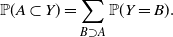 \begin{equation*} {\mathbb{P}}(A\subset Y) = \sum_{B\supset A} {\mathbb{P}}(Y = B). \end{equation*}
Using the Möbius inversion formula (see Appendix A), for all $A\subset{\mathcal{Y}}, $
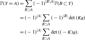 \begin{equation*}\begin{aligned} {\mathbb{P}}(Y = A) &= \sum_{B\supset A} (-1)^{|B\setminus A|} {\mathbb{P}}(B \subset Y) \\* &= (-1)^{|A|} \sum_{B\supset A} (-1)^{|B|} \det(K_B)\\*& = (-1)^{|A|} \sum_{B\supset A} \det((-K)_B){.}\end{aligned}\end{equation*}
Furthermore, Kulesza and Taskar [Reference Kulesza and Taskar27] state in their Theorem 2.1 that, for all $ L \in {\mathbb{R}}^{N \times N}$
,
$ L \in {\mathbb{R}}^{N \times N}$
,
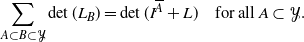 \begin{equation*}\sum_{A \subset B \subset \mathcal{Y}}\det(L_B) = \det(I^{\overline{A}}+L)\quad{\text{for all $A \subset \mathcal{Y}$}}.\end{equation*}
Then we obtain
 \begin{equation*} \hspace*{133pt}{\mathbb{P}}(Y = A) = (-1)^{|A|} \det(I^{\overline{A}} - K). \end{equation*}
By definition we have ${\mathbb{P}}(A \subset Y) = \det(K_A)$
for all A, and as a consequence
${\mathbb{P}}(A \subset Y) = \det(K_A)$
for all A, and as a consequence ${\mathbb{P}}(B \cap Y = \emptyset) = \det((I - K)_B)$
for all B. The next proposition gives, for any DPP, the expression of the general marginal
${\mathbb{P}}(B \cap Y = \emptyset) = \det((I - K)_B)$
for all B. The next proposition gives, for any DPP, the expression of the general marginal ${\mathbb{P}}(A \subset Y, B \cap Y = \emptyset)$
, for any A, B disjoint subsets of
${\mathbb{P}}(A \subset Y, B \cap Y = \emptyset)$
, for any A, B disjoint subsets of $\mathcal{Y}$
, using K. In what follows,
$\mathcal{Y}$
, using K. In what follows, $H^B$
denotes the symmetric positive semi-definite matrix
$H^B$
denotes the symmetric positive semi-definite matrix
 \begin{equation*}H^B = K + K_{{\mathcal{Y}} \times B} ((I-K)_B)^{-1} K_{B\times {\mathcal{Y}}}.\end{equation*}
Theorem 1. (General marginal of a DPP.) Let $A, B\subset{\mathcal{Y}}$
be disjoint. If
$A, B\subset{\mathcal{Y}}$
be disjoint. If
 \begin{equation*} {\mathbb{P}}(B\cap Y = \emptyset) = \det((I-K)_B) = 0, \end{equation*}
then
 \begin{equation*} {{\mathbb{P}}(A\subset Y, B\cap Y = \emptyset)=0}. \end{equation*}
Otherwise the matrix $(I-K)_B$
is invertible and
$(I-K)_B$
is invertible and
 \begin{equation*}{\mathbb{P}}(A\subset Y, B\cap Y = \emptyset) = \det((I-K)_B)\det(H^B_A).\end{equation*}
Proof. Let $A, B\subset{\mathcal{Y}}$
be disjoint such that
$A, B\subset{\mathcal{Y}}$
be disjoint such that ${\mathbb{P}}(B\cap Y = \emptyset) \neq 0$
. Using the above proposition,
${\mathbb{P}}(B\cap Y = \emptyset) \neq 0$
. Using the above proposition,
 \begin{equation*}{\mathbb{P}}(A\subset Y, B\cap Y = \emptyset)= \sum_{A\subset C \subset \overline{B}} {\mathbb{P}}(Y = C)= \sum_{A\subset C \subset \overline{B}} (-1)^{|C|} \det(I^{\overline{C}} - K).\end{equation*}
For any C such that $A\subset C \subset \overline{B}$
, we have
$A\subset C \subset \overline{B}$
, we have $B\subset \overline{C}$
. Hence, by reordering the matrix coefficients and using Schur’s determinant formula [Reference Horn and Johnson23],
$B\subset \overline{C}$
. Hence, by reordering the matrix coefficients and using Schur’s determinant formula [Reference Horn and Johnson23],
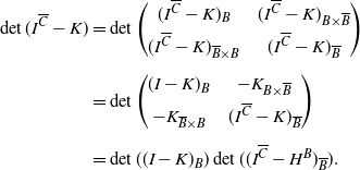 \begin{equation*}\begin{aligned}\det(I^{\overline{C}} - K)&= \det\begin{pmatrix}(I^{\overline{C}} - K)_B & \quad (I^{\overline{C}} - K)_{B\times \overline{B}} \\[4pt]
(I^{\overline{C}} - K)_{\overline{B}\times B} & \quad (I^{\overline{C}} - K)_{\overline{B}}\end{pmatrix}\\[5pt]
&= \det\begin{pmatrix}(I - K)_B & \quad -K_{B\times \overline{B}} \\[4pt]
-K_{\overline{B}\times B} & \quad (I^{\overline{C}} - K)_{\overline{B}}\end{pmatrix}\\[5pt]
&= \det((I - K)_B) \det(( I^{\overline{C}} - H^B)_{\overline{B}}).\end{aligned}\end{equation*}
\begin{equation*}\begin{aligned}\det(I^{\overline{C}} - K)&= \det\begin{pmatrix}(I^{\overline{C}} - K)_B & \quad (I^{\overline{C}} - K)_{B\times \overline{B}} \\[4pt]
(I^{\overline{C}} - K)_{\overline{B}\times B} & \quad (I^{\overline{C}} - K)_{\overline{B}}\end{pmatrix}\\[5pt]
&= \det\begin{pmatrix}(I - K)_B & \quad -K_{B\times \overline{B}} \\[4pt]
-K_{\overline{B}\times B} & \quad (I^{\overline{C}} - K)_{\overline{B}}\end{pmatrix}\\[5pt]
&= \det((I - K)_B) \det(( I^{\overline{C}} - H^B)_{\overline{B}}).\end{aligned}\end{equation*}
Thus
 \begin{equation*}{\mathbb{P}}(A\subset Y, B\cap Y = \emptyset)= \det((I - K)_B) \sum_{A\subset C \subset \overline{B}} (-1)^{|C|} \det( ( I^{\overline{C}} -H^B)_{\overline{B}}).\end{equation*}
According to Theorem 2.1 of Kulesza and Taskar [Reference Kulesza and Taskar27], for all $A\subset\overline{B}$
,
$A\subset\overline{B}$
,
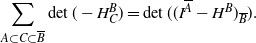 \begin{equation*}\quad \sum_{A\subset C \subset \overline{B}} \det( - H^B_C) = \det( ( I^{\overline{A}} -H^B)_{\overline{B}}).\end{equation*}
Then the Möbius inversion formula ensures that, for all $ A\subset\overline{B}$
,
$ A\subset\overline{B}$
,
 \begin{equation*}\sum_{A\subset C \subset \overline{B}} (-1)^{|C\setminus A|} \det( ( I^{\overline{C}} -H^B)_{\overline{B}})= \det( - H^B_A)= (-1)^{|A|} \det(H^B_A).\end{equation*}
Hence
 \begin{equation*} \hspace*{100pt} {\mathbb{P}}(A\subset Y, B\cap Y = \emptyset) = \det((I - K)_B) \det\big(H^B_A\big). \end{equation*}
With this formula, we can explicitly formulate the pointwise conditional probabilities of any DPP.
Corollary 1. (Pointwise conditional probabilities of a DPP.) Let $A, B\subset{\mathcal{Y}}$
be two disjoint sets such that
$A, B\subset{\mathcal{Y}}$
be two disjoint sets such that ${{\mathbb{P}}(A\subset Y,\, B\cap Y = \emptyset)\neq 0}$
, and let
${{\mathbb{P}}(A\subset Y,\, B\cap Y = \emptyset)\neq 0}$
, and let $k\notin A\cup B$
. Then
$k\notin A\cup B$
. Then
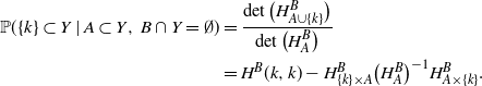 \begin{align}{\mathbb{P}}(\{k\}\subset Y \mid A \subset Y,\, B\cap Y = \emptyset)&= \frac{\det\big(H^B_{A\cup\{k\}}\big)}{\det\big(H^B_A\big)} \notag \\*&= H^B(k,k) - H^B_{\{k\}\times A} \big(H^B_A\big)^{-1} H^B_{A\times \{k\}}.\end{align}
This is a straightforward application of the previous expression and the Schur determinant formula [Reference Horn and Johnson23]. Note that these pointwise conditional probabilities are related to the Palm distribution of a point process [Reference Chiu, Stoyan, Kendall and Mecke12], which characterizes the distribution of the point process under the condition that there is a point at some location $x \in {\mathcal{Y}}$
. Shirai and Takahashi proved in [Reference Shirai and Takahashi41] that DPPs on general spaces are closed under Palm distributions, in the sense that there exists a DPP kernel
$x \in {\mathcal{Y}}$
. Shirai and Takahashi proved in [Reference Shirai and Takahashi41] that DPPs on general spaces are closed under Palm distributions, in the sense that there exists a DPP kernel $K^x$
such that the Palm measure associated to DPP(K) and x is a DPP defined on
$K^x$
such that the Palm measure associated to DPP(K) and x is a DPP defined on ${\mathcal{Y}}$
with kernel
${\mathcal{Y}}$
with kernel $K^x$
. Borodin and Rains [Reference Borodin and Rains9] also provide similar results on discrete spaces, using L-ensembles, that Kulesza and Taskar adapt in [Reference Kulesza and Taskar27]. They condition the DPP not only on a subset included in the point process but also, similarly to (1), on a subset not included in the point process. Like Shirai and Takahashi, they derive a formulation of the generated marginal kernel L.
$K^x$
. Borodin and Rains [Reference Borodin and Rains9] also provide similar results on discrete spaces, using L-ensembles, that Kulesza and Taskar adapt in [Reference Kulesza and Taskar27]. They condition the DPP not only on a subset included in the point process but also, similarly to (1), on a subset not included in the point process. Like Shirai and Takahashi, they derive a formulation of the generated marginal kernel L.
Now we have all the necessary expressions for the sequential sampling of a DPP.
2.2. Sequential sampling algorithm of a DPP
This sequential sampling algorithm simply consists in using (1) and updating the pointwise conditional probability at each step, knowing the previous selected points. It is presented in Algorithm 2. We recall that this sequential algorithm is the first step toward developing a competitive sampling algorithm for DPPs: with this method we no longer need eigendecomposition. The second step (Section 3) will be to reduce its computational cost.
Algorithm 2 Sequential sampling of a DPP with kernel K
The main operations of Algorithm 2 involve solving linear systems related to $(I-K)_B^{-1}$
. Fortunately, here we can use the Cholesky factorization, which alleviates the computational cost. Suppose that
$(I-K)_B^{-1}$
. Fortunately, here we can use the Cholesky factorization, which alleviates the computational cost. Suppose that $T^B$
is the Cholesky factorization of
$T^B$
is the Cholesky factorization of $(I-K)_B$
, that is,
$(I-K)_B$
, that is, $T^B$
is a lower triangular matrix such that
$T^B$
is a lower triangular matrix such that $(I-K)_B = T^B (T^{B})^{*}$
(where
$(I-K)_B = T^B (T^{B})^{*}$
(where $(T^{B})^{*}$
is the conjugate transpose of
$(T^{B})^{*}$
is the conjugate transpose of $T^{B}$
). Then, denoting
$T^{B}$
). Then, denoting $J^B = (T^{B})^{-1} K_{B\times A\cup\{k\}}$
, we simply have
$J^B = (T^{B})^{-1} K_{B\times A\cup\{k\}}$
, we simply have $H^B_{A\cup\{k\}} = K_{A\cup\{k\}} + (J^{B})^{*} J^B.$
Furthermore, at each iteration where B grows, the Cholesky decomposition $T^{B\cup\{k\}}$
of
$T^{B\cup\{k\}}$
of $(I-K)_{B\cup\{k\}}$
can be computed from
$(I-K)_{B\cup\{k\}}$
can be computed from $T^B$
using standard Cholesky update operations, involving the resolution of only one linear system of size
$T^B$
using standard Cholesky update operations, involving the resolution of only one linear system of size $|B|$
. See Appendix B for the details of a typical Cholesky decomposition update.
$|B|$
. See Appendix B for the details of a typical Cholesky decomposition update.
In comparison with the spectral sampling algorithm of Hough et al. [Reference Hough, Krishnapur, Peres and Virág24], we require computations for each site of ${\mathcal{Y}}$
, and not just one for each sampled point of Y. We will see at the end of Section 3 and in the experiments that it is not competitive.
${\mathcal{Y}}$
, and not just one for each sampled point of Y. We will see at the end of Section 3 and in the experiments that it is not competitive.
3. Sequential thinning algorithm
In this section we show that we can significantly decrease the number of steps and the running time of Algorithm 2: we propose first sampling a point process X containing Y, the desired DPP, and then making a sequential selection of the points of X to obtain Y. This procedure will be called a sequential thinning.
3.1 General framework of sequential thinning
We first describe a general sufficient condition for which a target point process Y – it will be a determinantal point process in our case – can be obtained as a sequential thinning of a point process X. This is a discrete adaptation of the thinning procedure on the continuous line of Rolski and Szekli [Reference Rolski and Szekli38]. To do this, we will consider a coupling (X, Z) such that $Z\subset X$
will be a random selection of the points of X and that will have the same distribution as Y. From this point onward, we identify the set X with the vector of size N with 1 in the place of the elements of X and 0 elsewhere, and we use the notations
$Z\subset X$
will be a random selection of the points of X and that will have the same distribution as Y. From this point onward, we identify the set X with the vector of size N with 1 in the place of the elements of X and 0 elsewhere, and we use the notations $X_{1:k}$
to denote the vector
$X_{1:k}$
to denote the vector $(X_1,\dots,X_k)$
and
$(X_1,\dots,X_k)$
and $0_{1:k}$
to denote the null vector of size k. We want to define the random vector
$0_{1:k}$
to denote the null vector of size k. We want to define the random vector $(X_1,Z_1,X_2,Z_2,\dots,X_N,Z_N)\in{\mathbb{R}}^{2N}$
with the following conditional distributions for
$(X_1,Z_1,X_2,Z_2,\dots,X_N,Z_N)\in{\mathbb{R}}^{2N}$
with the following conditional distributions for $X_k$
and
$X_k$
and $Z_k$
:
$Z_k$
:
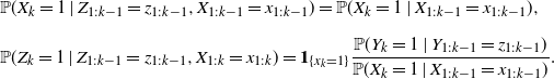 \begin{equation}\begin{aligned} & {\mathbb{P}}(X_k = 1\mid Z_{1:k-1} = z_{1:k-1}, X_{1:k-1} = x_{1:k-1}) = {\mathbb{P}}(X_k = 1\mid X_{1:k-1} = x_{1:k-1}) {,}\\[6pt]
& {\mathbb{P}}(Z_k = 1\mid Z_{1:k-1} = z_{1:k-1}, X_{1:k} = x_{1:k}) = \mathbf{1}_{\{x_k=1\}} \frac{{\mathbb{P}}(Y_k = 1\mid Y_{1:k-1} = z_{1:k-1})}{{\mathbb{P}}(X_k = 1\mid X_{1:k-1}=x_{1:k-1})}.\end{aligned}\end{equation}
\begin{equation}\begin{aligned} & {\mathbb{P}}(X_k = 1\mid Z_{1:k-1} = z_{1:k-1}, X_{1:k-1} = x_{1:k-1}) = {\mathbb{P}}(X_k = 1\mid X_{1:k-1} = x_{1:k-1}) {,}\\[6pt]
& {\mathbb{P}}(Z_k = 1\mid Z_{1:k-1} = z_{1:k-1}, X_{1:k} = x_{1:k}) = \mathbf{1}_{\{x_k=1\}} \frac{{\mathbb{P}}(Y_k = 1\mid Y_{1:k-1} = z_{1:k-1})}{{\mathbb{P}}(X_k = 1\mid X_{1:k-1}=x_{1:k-1})}.\end{aligned}\end{equation}
Proposition 2. (Sequential thinning.) Assume that X,Y, Z are discrete point processes on ${\mathcal{Y}}$
that satisfy, for all
${\mathcal{Y}}$
that satisfy, for all $k\in\{1,\dots,N\}$
and all z,
$k\in\{1,\dots,N\}$
and all z, $x\in\{0,1\}^N$
,
$x\in\{0,1\}^N$
,
 \begin{align}&{\mathbb{P}}(Z_{1:k-1}=z_{1:k-1},X_{1:k-1}=x_{1:k-1}) > 0\notag \\*\textit{implies}\quad &{\mathbb{P}}(Y_{k} = 1\mid Y_{1:k-1} = z_{1:k-1}) \leq {\mathbb{P}}(X_{k} = 1\mid X_{1:k-1}=x_{1:k-1}).\end{align}
Then it is possible to choose (X, Z) in such a way that (2) is satisfied. In that case Z is a thinning of X, i.e. $Z\subset X$
, and Z has the same distribution as Y.
$Z\subset X$
, and Z has the same distribution as Y.
Proof. Let us first discuss the definition of the coupling (X, Z). With the conditions (3), the ratios defining the conditional probabilities of (2) are ensured to be between 0 and 1 (if the conditional events have non-zero probabilities). Hence the conditional probabilities allow us to construct sequentially the distribution of the random vector $(X_1,Z_1,X_2,Z_2,\dots,X_N,Z_N)$
of length 2N, and thus the coupling is well-defined. Furthermore, as (2) is satisfied,
$(X_1,Z_1,X_2,Z_2,\dots,X_N,Z_N)$
of length 2N, and thus the coupling is well-defined. Furthermore, as (2) is satisfied, $Z_k = 1$
only if
$Z_k = 1$
only if $X_k =1$
, so we have
$X_k =1$
, so we have $Z\subset X$
.
$Z\subset X$
.
Let us now show that Z has the same distribution as Y. By complementarity of the events $\{Z_k = 0\}$
and
$\{Z_k = 0\}$
and $\{Z_k = 1\}$
, it is enough to show that for all
$\{Z_k = 1\}$
, it is enough to show that for all $k\in\{1,\dots,N\}$
, and
$k\in\{1,\dots,N\}$
, and $z_1,\dots,z_{k-1}$
such that
$z_1,\dots,z_{k-1}$
such that ${\mathbb{P}}(Z_{1:k-1} = z_{1:k-1})>0$
,
${\mathbb{P}}(Z_{1:k-1} = z_{1:k-1})>0$
,
 \begin{equation} {\mathbb{P}}(Z_k = 1\mid Z_{1:k-1} = z_{1:k-1}) = {\mathbb{P}}(Y_k = 1\mid Y_{1:k-1} = z_{1:k-1}).\end{equation}
Let $k\in\{1,\dots,N\}$
,
$k\in\{1,\dots,N\}$
, $(z_{1:k-1},x_{1:k-1}) \in\{0,1\}^{2(k-1)}$
, such that
$(z_{1:k-1},x_{1:k-1}) \in\{0,1\}^{2(k-1)}$
, such that
 \begin{equation*}{\mathbb{P}}(Z_{1:k-1}=z_{1:k-1},X_{1:k-1}=x_{1:k-1}) > 0.\end{equation*}
Since $Z \subset X$
,
$Z \subset X$
, $\{Z_k = 1\} = \{Z_k = 1, X_k = 1\}$
. Suppose first that
$\{Z_k = 1\} = \{Z_k = 1, X_k = 1\}$
. Suppose first that
 \begin{equation*} {\mathbb{P}}(X_k = 1\mid X_1 = x_1,\dots, X_{k-1} = x_{k-1})\neq 0. \end{equation*}
Then
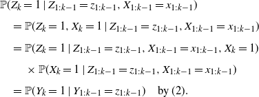 \begin{align*}& {\mathbb{P}}(Z_k = 1\mid Z_{1:k-1} = z_{1:k-1},X_{1:k-1}=x_{1:k-1})\\[4pt]
&\quad = {\mathbb{P}}(Z_k = 1,X_k = 1\mid Z_{1:k-1} = z_{1:k-1}, X_{1:k-1}=x_{1:k-1})\\[4pt]
&\quad ={\mathbb{P}}(Z_k = 1\mid Z_{1:k-1} = z_{1:k-1},X_{1:k-1}=x_{1:k-1},X_k = 1)\\[4pt]
&\quad \quad\, \times {\mathbb{P}}(X_k = 1\mid Z_{1:k-1} = z_{1:k-1}, X_{1:k-1}=x_{1:k-1})\\[4pt]
&\quad = {\mathbb{P}}(Y_k = 1\mid Y_{1:k-1} = z_{1:k-1})\quad \text{{by (\linkref{disp2}{2})}}.\end{align*}
\begin{align*}& {\mathbb{P}}(Z_k = 1\mid Z_{1:k-1} = z_{1:k-1},X_{1:k-1}=x_{1:k-1})\\[4pt]
&\quad = {\mathbb{P}}(Z_k = 1,X_k = 1\mid Z_{1:k-1} = z_{1:k-1}, X_{1:k-1}=x_{1:k-1})\\[4pt]
&\quad ={\mathbb{P}}(Z_k = 1\mid Z_{1:k-1} = z_{1:k-1},X_{1:k-1}=x_{1:k-1},X_k = 1)\\[4pt]
&\quad \quad\, \times {\mathbb{P}}(X_k = 1\mid Z_{1:k-1} = z_{1:k-1}, X_{1:k-1}=x_{1:k-1})\\[4pt]
&\quad = {\mathbb{P}}(Y_k = 1\mid Y_{1:k-1} = z_{1:k-1})\quad \text{{by (\linkref{disp2}{2})}}.\end{align*}
If ${\mathbb{P}}(X_k = 1\mid X_{1:k-1}=x_{1:k-1}) = 0$
, then
${\mathbb{P}}(X_k = 1\mid X_{1:k-1}=x_{1:k-1}) = 0$
, then
 \begin{equation*} {\mathbb{P}}(Z_k = 1\mid Z_{1:k-1} = z_{1:k-1},X_{1:k-1}=x_{1:k-1}) = 0{,} \end{equation*}
and using (3),
 \begin{equation*} {\mathbb{P}}(Y_k = 1\mid Y_{1:k} = z_{1:k}) =0. \end{equation*}
Hence the identity
 \begin{equation*} {\mathbb{P}}(Z_k = 1\mid Z_{1:k-1} = z_{1:k-1},X_{1:k-1}=x_{1:k-1}) = {\mathbb{P}}(Y_k = 1\mid Y_{1:k-1} = z_{1:k-1})\end{equation*}
is always valid. Since the values $x_1,\dots,x_{k-1}$
do not influence this conditional probability, one can conclude that given
$x_1,\dots,x_{k-1}$
do not influence this conditional probability, one can conclude that given $(Z_1,\dots,Z_{k-1})$
,
$(Z_1,\dots,Z_{k-1})$
, $Z_k$
is independent of
$Z_k$
is independent of $X_1,\dots,X_{k-1}$
, and thus (4) is true. □
$X_1,\dots,X_{k-1}$
, and thus (4) is true. □
The characterization of the thinning defined here allows both extreme cases: there can be no preselection of points by X, meaning that $X = {\mathcal{Y}}$
and that the DPP Y is sampled by Algorithm 2, or there can be no thinning at all, meaning that the final process Y can be equal to the dominating process X. Regarding sampling acceleration, a good dominating process X must be sampled quickly and with a cardinality as close as possible to
$X = {\mathcal{Y}}$
and that the DPP Y is sampled by Algorithm 2, or there can be no thinning at all, meaning that the final process Y can be equal to the dominating process X. Regarding sampling acceleration, a good dominating process X must be sampled quickly and with a cardinality as close as possible to $|Y|$
.
$|Y|$
.
3.2. Sequential thinning algorithm for DPPs
In this section we use the sequential thinning approach, where Y is a DPP of kernel K on the ground set ${\mathcal{Y}}$
, and X is a Bernoulli point process (BPP). BPPs are the fastest and easiest point processes to sample. X is a Bernoulli process if the components of the vector
${\mathcal{Y}}$
, and X is a Bernoulli point process (BPP). BPPs are the fastest and easiest point processes to sample. X is a Bernoulli process if the components of the vector $(X_1,\dots, X_N)$
are independent. Its distribution is determined by the probability of occurrence of each point k, which we denote by
$(X_1,\dots, X_N)$
are independent. Its distribution is determined by the probability of occurrence of each point k, which we denote by $q_k = {\mathbb{P}}(X_k=1)$
. Due to the independence property, (3) simplifies to
$q_k = {\mathbb{P}}(X_k=1)$
. Due to the independence property, (3) simplifies to
 \begin{equation*}{\mathbb{P}}(Z_{1:k-1}=z_{1:k-1},X_{1:k-1}=x_{1:k-1}) > 0\quad \text{implies} \quad{\mathbb{P}}(Y_k = 1\mid Y_{1:k-1} = z_{1:k-1}) \leq q_k.\end{equation*}
The second inequality does not depend on x, so it must be valid as soon as there exists a vector x such that ${\mathbb{P}}(Z_{1:k-1}=z_{1:k-1},X_{1:k-1}=x_{1:k-1}) > 0$
, that is, as soon as
${\mathbb{P}}(Z_{1:k-1}=z_{1:k-1},X_{1:k-1}=x_{1:k-1}) > 0$
, that is, as soon as ${\mathbb{P}}(Z_{1:k-1}=z_{1:k-1})>0$
. Since we want Z to have the same distribution as Y, we finally obtain the conditions
${\mathbb{P}}(Z_{1:k-1}=z_{1:k-1})>0$
. Since we want Z to have the same distribution as Y, we finally obtain the conditions
 \begin{equation*} {\mathbb{P}}(Y_{1:k-1}=y_{1:k-1})>0 \quad \text{implies}\quad{\mathbb{P}}(Y_k = 1\mid Y_{1:k-1}=y_{1:k-1}) \leq q_k\quad {\text{for all $y\in\{0,1\}^N$}.}\end{equation*}
Ideally, we want the $q_k$
to be as small as possible to ensure that the cardinality of X is as small as possible. So we look for the optimal values
$q_k$
to be as small as possible to ensure that the cardinality of X is as small as possible. So we look for the optimal values $q_k^*$
, that is,
$q_k^*$
, that is,
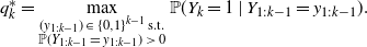 \begin{equation*}q_k^*=\max_{\substack{(y_{1:k-1})\;\in\;\{0,1\}^{k-1}\;\text{s.t.}\\\mathbb{P}(Y_{1:k-1}\; =\; y_{1:k-1})\;>\;0}}{\mathbb{P}}(Y_k = 1\mid Y_{1:k-1} = y_{1:k-1}).\end{equation*}
A priori, computing $q_k^*$
would raise combinatorial issues. However, due to the repulsive nature of DPPs, we have the following proposition.
$q_k^*$
would raise combinatorial issues. However, due to the repulsive nature of DPPs, we have the following proposition.
Proposition 3. Let $A, B\subset{\mathcal{Y}}$
be two disjoint sets such that
$A, B\subset{\mathcal{Y}}$
be two disjoint sets such that ${\mathbb{P}}(A\subset Y,\, B\cap Y = \emptyset)\neq 0$
, and let
${\mathbb{P}}(A\subset Y,\, B\cap Y = \emptyset)\neq 0$
, and let $k \neq l \in \overline{A\cup B}$
. If
$k \neq l \in \overline{A\cup B}$
. If ${\mathbb{P}}(A\cup\{l\} \subset Y,\, B\cap Y = \emptyset) >0$
, then
${\mathbb{P}}(A\cup\{l\} \subset Y,\, B\cap Y = \emptyset) >0$
, then
 \begin{equation*}{\mathbb{P}}(\{k\}\subset Y \mid A\cup\{l\} \subset Y,\, B\cap Y = \emptyset)\leq {\mathbb{P}}(\{k\}\subset Y \mid A \subset Y,\, B\cap Y = \emptyset).\end{equation*}
If ${\mathbb{P}}(A \subset Y,\, (B\cup\{l\})\cap Y = \emptyset) >0$
, then
${\mathbb{P}}(A \subset Y,\, (B\cup\{l\})\cap Y = \emptyset) >0$
, then
 \begin{equation*}{\mathbb{P}}(\{k\}\subset Y \mid A \subset Y,\, (B\cup\{l\})\cap Y = \emptyset)\geq {\mathbb{P}}(\{k\}\subset Y \mid A \subset Y,\, B\cap Y = \emptyset).\end{equation*}
Consequently, for all $k\in{\mathcal{Y}}$
, if
$k\in{\mathcal{Y}}$
, if $y_{1:k-1} \leq z_{1:k-1}$
(where
$y_{1:k-1} \leq z_{1:k-1}$
(where $\leq$
stands for the inclusion partial order) are two states for
$\leq$
stands for the inclusion partial order) are two states for $Y_{1:k-1}$
, then
$Y_{1:k-1}$
, then
 \begin{equation*}{\mathbb{P}}(Y_k = 1\mid Y_{1:k-1} = y_{1:k-1}) \geq {\mathbb{P}}(Y_k = 1\mid Y_{1:k-1} = z_{1:k-1}).\end{equation*}
In particular, for all $k \in \{1,\dots, N \}$
, if
$k \in \{1,\dots, N \}$
, if ${\mathbb{P}}(Y_{1:k-1} = 0_{1:k-1}) > 0$
then
${\mathbb{P}}(Y_{1:k-1} = 0_{1:k-1}) > 0$
then
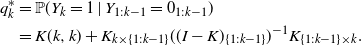 \begin{align*}q_k^*&= {\mathbb{P}}(Y_k = 1\mid Y_{1:k-1} = 0_{1:k-1})\\&= K(k,k) + K_{k \times \{1:k-1\}} ((I-K)_{\{1:k-1\}})^{-1} K_{ \{1:k-1\}\times k}.\end{align*}
Proof. Recall that by Proposition 1,
 \begin{equation*}P(\{k\}\subset Y \mid A \subset Y,\, B\cap Y = \emptyset)= H^B(k,k) - H^B_{\{k\}\times A} (H^B_A)^{-1} H^B_{A\times \{k\}}.\end{equation*}
Let $l \notin A\cup B\cup\{k\}$
. Consider
$l \notin A\cup B\cup\{k\}$
. Consider $T^B$
the Cholesky decomposition of the matrix
$T^B$
the Cholesky decomposition of the matrix $H^B$
obtained with the following ordering of the coefficients: A, l, the remaining coefficients of
$H^B$
obtained with the following ordering of the coefficients: A, l, the remaining coefficients of ${\mathcal{Y}}\setminus(A\cup\{l\})$
. Then the restriction
${\mathcal{Y}}\setminus(A\cup\{l\})$
. Then the restriction $T^B_A$
is the Cholesky decomposition (of the reordered)
$T^B_A$
is the Cholesky decomposition (of the reordered) $H^B_A$
, and thus
$H^B_A$
, and thus
 \begin{equation*}H^B_{\{k\}\times A} (H^B_A)^{-1} H^B_{A\times \{k\}}= H^B_{\{k\}\times A} (T^B_A(T^B_A)^*)^{-1} H^B_{A\times \{k\}}= \|(T^B_A)^{-1} H^B_{A\times \{k\}}\|_2^2.\end{equation*}
Similarly,
 \begin{equation*}H^B_{\{k\}\times A\cup\{l\}} (H^B_{A\cup\{l\}})^{-1} H^B_{A\cup\{l\}\times \{k\}}= \|(T^B_{A\cup\{l\}})^{-1} H^B_{A\cup\{l\}\times \{k\}}\|_2^2.\end{equation*}
Now note that solving the triangular system with $b = (T^B_{A\cup\{l\}})^{-1} H^B_{A\cup\{l\}\times \{k\}}$
amounts to solving the triangular system with
$b = (T^B_{A\cup\{l\}})^{-1} H^B_{A\cup\{l\}\times \{k\}}$
amounts to solving the triangular system with $(T^B_A)^{-1} H^B_{A\times \{k\}}$
and an additional line at the bottom. Hence we obtain
$(T^B_A)^{-1} H^B_{A\times \{k\}}$
and an additional line at the bottom. Hence we obtain
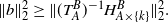 \begin{equation*}\|b\|_2^2\geq \|(T^B_A)^{-1} H^B_{A\times \{k\}}\|_2^2.\end{equation*}
Consequently, provided that ${\mathbb{P}}(A\cup\{l\} \subset Y,\, B\cap Y = \emptyset)>0$
, we have
${\mathbb{P}}(A\cup\{l\} \subset Y,\, B\cap Y = \emptyset)>0$
, we have
 \begin{equation*}{\mathbb{P}}(\{k\}\subset Y \mid A\cup\{l\} \subset Y,\, B\cap Y = \emptyset)\leq {\mathbb{P}}(\{k\}\subset Y \mid A \subset Y,\, B\cap Y = \emptyset).\end{equation*}
The second inequality is obtained by complementarity in applying the above inequality to the DPP $\overline{Y}$
with
$\overline{Y}$
with $B\cup\{l\} \subset \overline{Y}$
and
$B\cup\{l\} \subset \overline{Y}$
and $A\cap \overline{Y} = \emptyset$
. □
$A\cap \overline{Y} = \emptyset$
. □
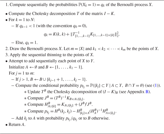
As a consequence, an admissible choice for the distribution of the Bernoulli process is
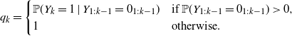 \begin{equation}q_k =\begin{cases}{\mathbb{P}}(Y_k=1\mid Y_{1:k-1} = 0_{1:k-1}) & \text{if } {\mathbb{P}}(Y_{1:k-1} = 0_{1:k-1})>0,\\1 & \text{otherwise}.\end{cases}\end{equation}
Note that if, for some index k, ${\mathbb{P}}(Y_{1:k-1} = 0_{1:k-1})>0$
is not satisfied, then for all the subsequent indexes
${\mathbb{P}}(Y_{1:k-1} = 0_{1:k-1})>0$
is not satisfied, then for all the subsequent indexes $l\geq k$
,
$l\geq k$
, $q_l=1$
, that is, the Bernoulli process becomes degenerate and contains all the points after k. In the remainder of this section, X will denote a Bernoulli process with probabilities
$q_l=1$
, that is, the Bernoulli process becomes degenerate and contains all the points after k. In the remainder of this section, X will denote a Bernoulli process with probabilities $(q_k)$
given by (5).
$(q_k)$
given by (5).
As discussed in the previous section, in addition to being easily simulated, one would like the cardinality of X to be close to the one of Y, the final sample. The next proposition shows that this is verified if all the eigenvalues of K are strictly less than 1.
Proposition 4. ( $|X|$
is proportional to
$|X|$
is proportional to $|Y|$
.) Suppose that
$|Y|$
.) Suppose that $P(Y = \emptyset) = \det(I-K) >0$
and let
$P(Y = \emptyset) = \det(I-K) >0$
and let $\lambda_{\max}(K)\in[0,1)$
denote the maximal eigenvalue of K. Then
$\lambda_{\max}(K)\in[0,1)$
denote the maximal eigenvalue of K. Then
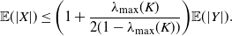 \begin{equation}\mathbb{E}(|X|) \leq \biggl(1 + \frac{\lambda_{\max}(K)}{2 (1-\lambda_{\max}(K))} \biggr) \mathbb{E}(|Y|).\end{equation}
Proof. We know that
 \begin{equation*}q_k = K(k,k) + K_{\{k\}\times\{1:k-1\}} ((I-K)_{\{1:k-1\}})^{-1}K_{\{1:k-1\}\times\{k\}},\end{equation*}
by Proposition 1. Since
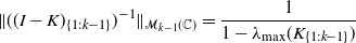 \begin{equation*}\|((I-K)_{\{1:k-1\}})^{-1}\|_{\mathcal{M}_{k-1}({\mathbb{C}})}= \frac{1}{1 - \lambda_{\max}(K_{\{1:k-1\}})}\end{equation*}
and $\lambda_{\max}(K_{\{1:k-1\}}) \leq \lambda_{\max}(K)$
, we have
$\lambda_{\max}(K_{\{1:k-1\}}) \leq \lambda_{\max}(K)$
, we have
 \begin{equation*} K_{\{k\}\times\{1:k-1\}} ((I-K)_{\{1:k-1\}})^{-1}K_{\{1:k-1\}\times\{k\}} \leq \frac{1}{1-\lambda_{\max}(K)} \|K_{\{1:k-1\}\times\{k\}}\|_2^2.\end{equation*}
Summing all these inequalities gives
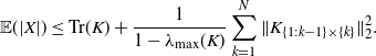 \begin{equation*}\mathbb{E}(|X|)\leq {\operatorname{Tr}}(K) + \frac{1}{1-\lambda_{\max}(K)} \sum_{k=1}^{N} \|K_{\{1:k-1\}\times\{k\}}\|_2^2.\end{equation*}
The last term is the Frobenius norm of the upper triangular part of K, so it can be bounded by
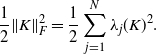 \begin{equation*}\frac{1}{2} \|K\|^2_{F} = \frac{1}{2} \sum_{j=1}^N \lambda_j(K)^2.\end{equation*}
Since $\lambda_j(K)^2 \leq \lambda_j(K)\lambda_{\max}(K)$
, we obtain
$\lambda_j(K)^2 \leq \lambda_j(K)\lambda_{\max}(K)$
, we obtain
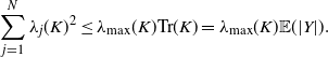 \begin{equation*} \hspace*{90pt} \sum_{j=1}^N \lambda_j(K)^2 \leq \lambda_{\max}(K) {\operatorname{Tr}}(K) = \lambda_{\max}(K) \mathbb{E}(|Y|). \end{equation*}
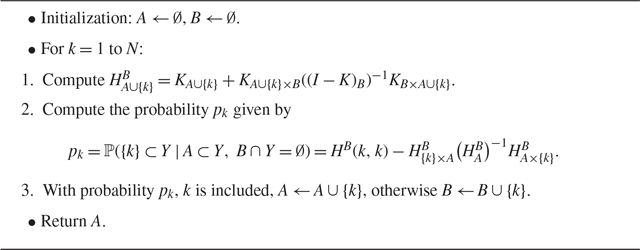
We can now introduce the final sampling algorithm, which we call the sequential thinning algorithm (Algorithm 3). It presents the different steps of our sequential thinning algorithm to sample a DPP of kernel K. The first step is a preprocess that must be done only once for a given matrix K. Step 2 is trivial and fast. The critical point is to sequentially compute the conditional probabilities $p_k = {\mathbb{P}}(\{k\}\subset Y \mid A \subset Y,\, B\cap Y = \emptyset)$
for each point of X. Recall that in Algorithm 2 we use a Cholesky decomposition of the matrix
$p_k = {\mathbb{P}}(\{k\}\subset Y \mid A \subset Y,\, B\cap Y = \emptyset)$
for each point of X. Recall that in Algorithm 2 we use a Cholesky decomposition of the matrix $(I-K)_B$
, which is updated by adding a line each time a point is added in B. Here the inverse of the matrix
$(I-K)_B$
, which is updated by adding a line each time a point is added in B. Here the inverse of the matrix $(I-K)_B$
is only needed when visiting a point
$(I-K)_B$
is only needed when visiting a point $k\in X$
, so we update the Cholesky decomposition by a single block, where the new block corresponds to all indices added to B in one iteration (see Appendix B). The MATLAB® implementation used for the experiments is available online (https://www.math-info.univ-paris5.fr/~claunay/exact_sampling.html), together with a Python version of this code, using the PyTorch library. Note that very recently Guillaume Gautier [Reference Gautier16] proposed an alternative computation of the Bernoulli probabilities, that generate the dominating point process in the first step of Algorithm 3, so that it only requires the diagonal coefficients of the Cholesky decomposition T of
$k\in X$
, so we update the Cholesky decomposition by a single block, where the new block corresponds to all indices added to B in one iteration (see Appendix B). The MATLAB® implementation used for the experiments is available online (https://www.math-info.univ-paris5.fr/~claunay/exact_sampling.html), together with a Python version of this code, using the PyTorch library. Note that very recently Guillaume Gautier [Reference Gautier16] proposed an alternative computation of the Bernoulli probabilities, that generate the dominating point process in the first step of Algorithm 3, so that it only requires the diagonal coefficients of the Cholesky decomposition T of $I-K$
.
$I-K$
.
Algorithm 3 Sequential thinning algorithm of a DPP with kernel K
3.3. Computational complexity
Recall that the size of the ground set ${\mathcal{Y}}$
is N and the size of the final sample is
${\mathcal{Y}}$
is N and the size of the final sample is $|Y|=n$
. Both algorithms introduced in this paper have running complexities of order
$|Y|=n$
. Both algorithms introduced in this paper have running complexities of order ${\text{O}}(N^3)$
, as the spectral algorithm. However, if we get into the details, the most expensive task in the spectral algorithm is the computation of the eigenvalues and the eigenvectors of the kernel K. As this matrix is Hermitian, the common routine for doing so is the reduction of K to some tridiagonal matrix to which the QR decomposition is applied, meaning that it is decomposed into the product of an orthogonal matrix and an upper triangular matrix. When N is large, the total number of operations is approximately
${\text{O}}(N^3)$
, as the spectral algorithm. However, if we get into the details, the most expensive task in the spectral algorithm is the computation of the eigenvalues and the eigenvectors of the kernel K. As this matrix is Hermitian, the common routine for doing so is the reduction of K to some tridiagonal matrix to which the QR decomposition is applied, meaning that it is decomposed into the product of an orthogonal matrix and an upper triangular matrix. When N is large, the total number of operations is approximately $\frac{4}{3}N^3$
[Reference Trefethen and Bau42]. In Algorithms 2 and 3, one of the most expensive operations is the Cholesky decomposition of several matrices. We recall that the Cholesky decomposition of a matrix of size
$\frac{4}{3}N^3$
[Reference Trefethen and Bau42]. In Algorithms 2 and 3, one of the most expensive operations is the Cholesky decomposition of several matrices. We recall that the Cholesky decomposition of a matrix of size $N\times N$
costs approximately
$N\times N$
costs approximately $\frac{1}{3}N^3$
computations when N is large [Reference Mayers and Süli34]. Concerning the sequential Algorithm 2, at each iteration k, the number of operations needed is of order
$\frac{1}{3}N^3$
computations when N is large [Reference Mayers and Süli34]. Concerning the sequential Algorithm 2, at each iteration k, the number of operations needed is of order $|B|^2|A| + |B||A|^2 + |A|^3$
, where
$|B|^2|A| + |B||A|^2 + |A|^3$
, where $|A|$
is the number of selected points at step k so it is lower than n, and
$|A|$
is the number of selected points at step k so it is lower than n, and $|B|$
is the number of unselected points, bounded by k. Then, when N tends to infinity, the total number of operations in Algorithm 2 is lower than
$|B|$
is the number of unselected points, bounded by k. Then, when N tends to infinity, the total number of operations in Algorithm 2 is lower than
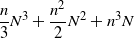 \begin{equation*}\frac{n}{3}N^3 + \frac{n^2}{2}N^2 + n^3N\end{equation*}
or ${\text{O}}(nN^3)$
, as in general
${\text{O}}(nN^3)$
, as in general $n \ll N$
. Concerning Algorithm 3, the sequential thinning from X, coming from Algorithm 2, costs
$n \ll N$
. Concerning Algorithm 3, the sequential thinning from X, coming from Algorithm 2, costs ${\text{O}}(n|X|^3)$
. Recall that
${\text{O}}(n|X|^3)$
. Recall that $|X|$
is proportional to
$|X|$
is proportional to $|Y|=n$
when the eigenvalues of K are smaller than 1 (see (6)) so this step costs
$|Y|=n$
when the eigenvalues of K are smaller than 1 (see (6)) so this step costs ${\text{O}}(n^4)$
. Then the Cholesky decomposition of
${\text{O}}(n^4)$
. Then the Cholesky decomposition of $I-K$
is the most expensive operation in Algorithm 3 as it costs approximately
$I-K$
is the most expensive operation in Algorithm 3 as it costs approximately $\frac{1}{3}N^3$
. In this case the overall running complexity of the sequential thinning algorithm is of order
$\frac{1}{3}N^3$
. In this case the overall running complexity of the sequential thinning algorithm is of order $\frac{1}{3}N^3$
, which is four times less than the spectral algorithm. When some eigenvalues of K are equal to 1, equation (6) no longer holds, so in that case the running complexity of Algorithm 3 is only bounded by
$\frac{1}{3}N^3$
, which is four times less than the spectral algorithm. When some eigenvalues of K are equal to 1, equation (6) no longer holds, so in that case the running complexity of Algorithm 3 is only bounded by ${\text{O}}(nN^3)$
.
${\text{O}}(nN^3)$
.
We will retrieve this experimentally as, depending on the application or on the kernel K, Algorithm 3 is able to speed up the sampling of DPPs. Note that in the above computations we have not taken into account the possible parallelization of the sequential thinning algorithm. As a matter of fact, the Cholesky decomposition is parallelizable [Reference George, Heath and Liu19]. Incorporating these parallel computations would probably speed up the sequential thinning algorithm, since the Cholesky decomposition of $I-K$
is the most expensive operation when the expected cardinality
$I-K$
is the most expensive operation when the expected cardinality $|Y|$
is low. The last part of the algorithm, the thinning procedure, operates sequentially, so it is not parallelizable. These comments on the complexity and running times depend on the implementation, on the choice of the programming language and speed-up strategies, so they mainly serve as an illustration.
$|Y|$
is low. The last part of the algorithm, the thinning procedure, operates sequentially, so it is not parallelizable. These comments on the complexity and running times depend on the implementation, on the choice of the programming language and speed-up strategies, so they mainly serve as an illustration.
4. Experiments
4.1. DPP models for runtime tests
In the following section we use the common notation of L-ensembles, with matrix $L = K(I-K)^{-1}$
. We present the results using four different kernels.
$L = K(I-K)^{-1}$
. We present the results using four different kernels.
(a) A random kernel. $ K = Q^{-1}DQ$
, where D is a diagonal matrix with uniformly distributed random values in (0, 1) and Q is a unitary matrix created from the QR decomposition of a random matrix.
$ K = Q^{-1}DQ$
, where D is a diagonal matrix with uniformly distributed random values in (0, 1) and Q is a unitary matrix created from the QR decomposition of a random matrix.-
(b) A discrete analog to the Ginibre kernel.
$K = L(I+L)^{-1}$
where, for all
$x_1, x_2 \in {\mathcal{Y}}= \{1,\dots,N \}$
,
\begin{equation*}L(x_1,x_2) = \frac{1}{\pi} \,{\text{e}}^{ -\frac{1}{2}( |x_1|^2 +|x_2|^2) + x_1 x_2}.\end{equation*}
-
(c) A patch-based kernel. Let u be a discrete image and
${\mathcal{Y}} = \mathcal{P}$
a subset of all its patches, i.e. square sub-images of size
$w\times w$
in u. Define
$K = L(I+L)^{-1}$
where, for all
$ P_1, P_2 \in \mathcal{P}$
,
where
\begin{equation*}L(P_1,P_2) = \exp\biggl(-\frac{\|P_1-P_2\|_2^2}{s^2}\biggr){,}\end{equation*}
$s>0$
is called the bandwidth or scale parameter. We will detail the definition and use of this kernel in Section 4.3.
-
(d) A projection kernel.
$ K = Q^{-1}DQ$
, where D is a diagonal matrix with the n first coefficients equal to 1 and the others equal to 0, and Q is a random unitary matrix as for model (a).


It is often essential to control the expected cardinality of the point process. For case (d) the cardinality is fixed to n. For the other three cases we use a procedure similar to the one developed in [Reference Barthelmé, Amblard and Tremblay7]. Recall that if $Y \sim {\operatorname{DPP}}(K)$
and
$Y \sim {\operatorname{DPP}}(K)$
and $K = L(I+L)^{-1}$
,
$K = L(I+L)^{-1}$
,
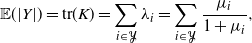 \begin{equation*}\mathbb{E}(|Y|) = {\operatorname{tr}}(K) = \sum_{i \in {\mathcal{Y}}} \lambda_i = \sum_{i \in {\mathcal{Y}}} \frac{\mu_i}{1+\mu_i} ,\end{equation*}
where $(\lambda_i)_{i \in {\mathcal{Y}}}$
are the eigenvalues of K and
$(\lambda_i)_{i \in {\mathcal{Y}}}$
are the eigenvalues of K and $(\mu_i)_{i \in {\mathcal{Y}}}$
are the eigenvalues of L [Reference Hough, Krishnapur, Peres and Virág24, Reference Kulesza and Taskar27]. Given an initial matrix
$(\mu_i)_{i \in {\mathcal{Y}}}$
are the eigenvalues of L [Reference Hough, Krishnapur, Peres and Virág24, Reference Kulesza and Taskar27]. Given an initial matrix $L = K(I-K)^{-1}$
and a desired expected cardinality
$L = K(I-K)^{-1}$
and a desired expected cardinality $\mathbb{E}(|Y|) = n$
, we run a binary search algorithm to find
$\mathbb{E}(|Y|) = n$
, we run a binary search algorithm to find $\alpha > 0$
such that
$\alpha > 0$
such that
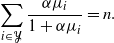 \begin{equation*}\sum_{i \in {\mathcal{Y}}} \frac{\alpha \mu_i}{1+\alpha \mu_i} = n.\end{equation*}
Then we use the kernels $L_{\alpha} = \alpha L$
and
$L_{\alpha} = \alpha L$
and $K_{\alpha} = L_{\alpha}(I+L_{\alpha} )^{-1}$
.
$K_{\alpha} = L_{\alpha}(I+L_{\alpha} )^{-1}$
.
4.2. Runtimes
For the following experiments, we ran the algorithms on a laptop HP Intel(R) Core(TM) i7-6600U CPU and we used the software MATLAB® R2018b. Note that the computational time results depend on the programming language and the use of optimized functions by the software. Thus the following numerical results are mainly indicative.
First let us compare the sequential thinning algorithm (Algorithm 3) presented here with the two main sampling algorithms: the classic spectral algorithm (Algorithm 1) and the ‘naive’ sequential algorithm (Algorithm 2). Figure 1 presents the running times of the three algorithms as a function of the total number of points of the ground set. Here we have chosen a patch-based kernel (c). The expected cardinality $\mathbb{E}(|Y|)$
is constant, equal to 20. As predicted, the sequential algorithm (Algorithm 2) is far slower than the two others. Whatever the chosen kernel and the expected cardinality of the DPP, this algorithm is not competitive. Note that the sequential thinning algorithm uses this sequential method after sampling the particular Bernoulli process. But we will see that this first dominating step can be very efficient and lead to a relatively fast algorithm.
$\mathbb{E}(|Y|)$
is constant, equal to 20. As predicted, the sequential algorithm (Algorithm 2) is far slower than the two others. Whatever the chosen kernel and the expected cardinality of the DPP, this algorithm is not competitive. Note that the sequential thinning algorithm uses this sequential method after sampling the particular Bernoulli process. But we will see that this first dominating step can be very efficient and lead to a relatively fast algorithm.
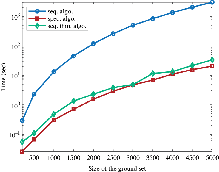
Figure 1: Running times of the three studied algorithms as a function of the size of the ground set, using a patch-based kernel.
From now on, we restrict the comparison to the spectral and sequential thinning algorithms (Algorithms 1 and 3). In Figures 2 and 3 we present the running times of these algorithms as a function of the size of $|{\mathcal{Y}}|$
in various situations. Figure 2 shows the running times when the expectation of the number of sampled points
$|{\mathcal{Y}}|$
in various situations. Figure 2 shows the running times when the expectation of the number of sampled points $\mathbb{E}(|Y|)$
is equal to 4% of the size of
$\mathbb{E}(|Y|)$
is equal to 4% of the size of ${\mathcal{Y}}$
: it increases as the total number of points increases. In this case we can see that whatever the chosen kernel, the spectral algorithm is faster as the complexity of sequential part of Algorithm 3 depends on the size
${\mathcal{Y}}$
: it increases as the total number of points increases. In this case we can see that whatever the chosen kernel, the spectral algorithm is faster as the complexity of sequential part of Algorithm 3 depends on the size $|X|$
that also grows. In Figure 3, as
$|X|$
that also grows. In Figure 3, as $|{\mathcal{Y}}|$
grows,
$|{\mathcal{Y}}|$
grows, $\mathbb{E}(|Y|)$
is fixed at 20. Except for the right-hand side kernel, we are in the configuration where
$\mathbb{E}(|Y|)$
is fixed at 20. Except for the right-hand side kernel, we are in the configuration where $|X|$
stays proportional to
$|X|$
stays proportional to $|Y|$
; then the Bernoulli step of Algorithm 3 is very efficient and this sequential thinning algorithm becomes competitive with the spectral algorithm. For these general kernels, we observe that the sequential thinning algorithm can be as fast as the spectral algorithm, and even faster when the expected cardinality of the sample is small compared to the size of the ground set. The question is: When and up to which expected cardinality is Algorithm 3 faster?
$|Y|$
; then the Bernoulli step of Algorithm 3 is very efficient and this sequential thinning algorithm becomes competitive with the spectral algorithm. For these general kernels, we observe that the sequential thinning algorithm can be as fast as the spectral algorithm, and even faster when the expected cardinality of the sample is small compared to the size of the ground set. The question is: When and up to which expected cardinality is Algorithm 3 faster?
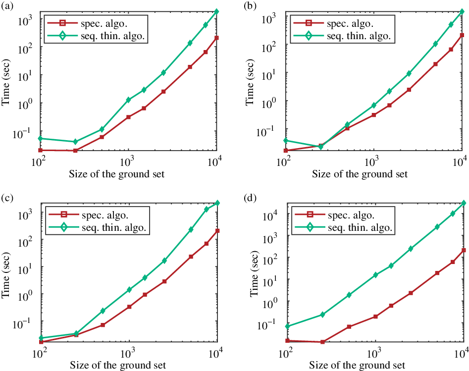
Figure 2: Running times in log-scale of the spectral and sequential thinning algorithms as a function of the size of the ground set $|{\mathcal{Y}}|$
, using ‘classic’ DPP kernels: (a) a random kernel, (b) a Ginibre-like kernel, (c) a patch-based kernel, and (d) a projection kernel. The expectation of the number of sampled points is set to
$|{\mathcal{Y}}|$
, using ‘classic’ DPP kernels: (a) a random kernel, (b) a Ginibre-like kernel, (c) a patch-based kernel, and (d) a projection kernel. The expectation of the number of sampled points is set to $4 \%$
of
$4 \%$
of $|{\mathcal{Y}}|$
.
$|{\mathcal{Y}}|$
.
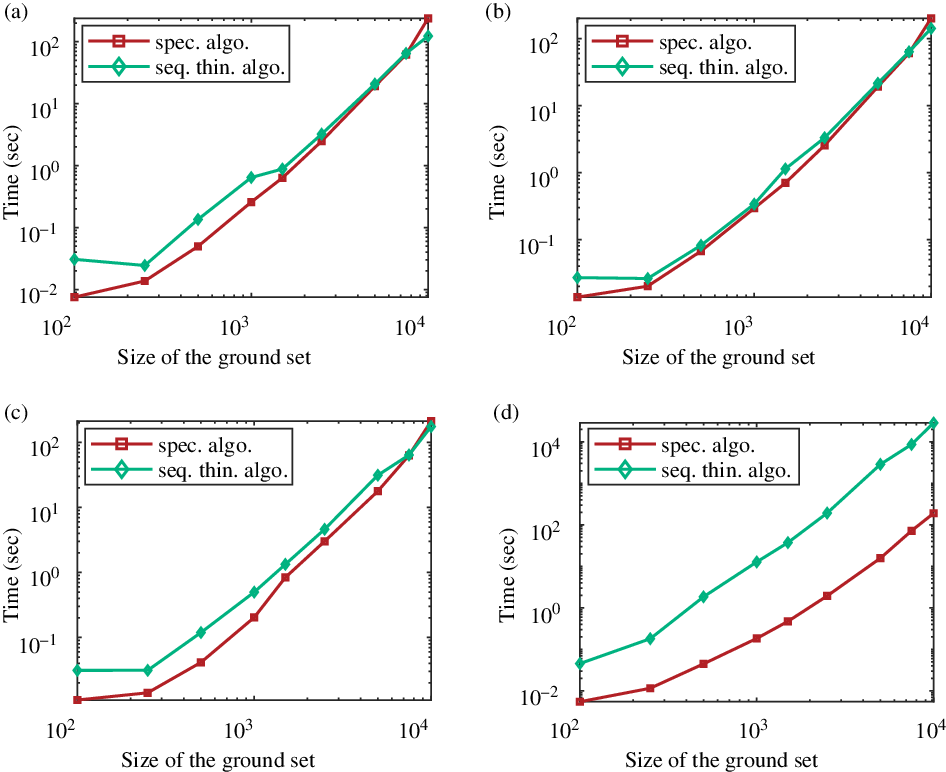
Figure 3: Running times in log-scale of the spectral and sequential thinning algorithms as a function of the size of the ground set $|{\mathcal{Y}}|$
, using ‘classic’ DPP kernels: (a) a random kernel, (b) a Ginibre-like kernel, (c) a patch-based kernel, and (d) a projection kernel. As
$|{\mathcal{Y}}|$
, using ‘classic’ DPP kernels: (a) a random kernel, (b) a Ginibre-like kernel, (c) a patch-based kernel, and (d) a projection kernel. As $|{\mathcal{Y}}|$
grows,
$|{\mathcal{Y}}|$
grows, $\mathbb{E}(|Y|)$
is constant, equal to 20.
$\mathbb{E}(|Y|)$
is constant, equal to 20.
Figure 4 displays the running times of both algorithms as a function of the expected cardinality of the sample when the size of the ground set is constant, equal to 5000 points. Note that, concerning the three left-hand side general kernels with no eigenvalue equal to one, the sequential thinning algorithm is faster under a certain expected number of points – which depends on the kernel. For instance, when the kernel is randomly defined and the range of desired points to sample is below 25, it is relevant to use this algorithm. To conclude, when the eigenvalues of the kernel are below one, Algorithm 3 seems relevant for large data sets but small samples. This case is quite common, for instance to summarize a text, to work only with representative points in clusters, or to denoise an image with a patch-based method.
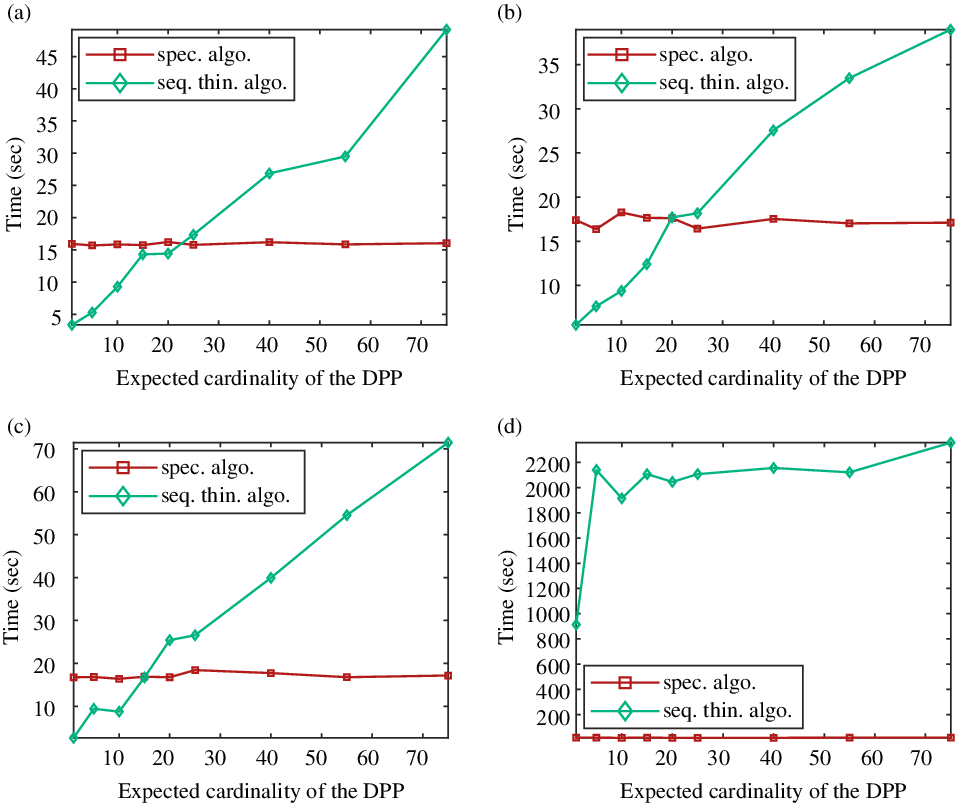
Figure 4: Running times of the spectral and sequential thinning algorithms as a function of the expected cardinality of the process, using (a) a random kernel, (b) a Ginibre-like kernel, (c) a patch-based kernel, and (d) a projection kernel. The size of the ground set is fixed to 5000 in all examples.
The projection kernel (when the eigenvalues of K are either 0 or 1) is, as expected, a complicated case. Figure 3(d) shows that our algorithm is not competitive when using this kernel. Indeed, the cardinality of the dominating Bernoulli process X can be very large. In this case the bound in (6) is not valid (and even tends to infinity) as $\lambda_{\max} = 1$
, and we necessarily reach the degenerated case when, after some index k, all the Bernoulli probabilities
$\lambda_{\max} = 1$
, and we necessarily reach the degenerated case when, after some index k, all the Bernoulli probabilities $q_l, l \geq k,$
are equal to 1. Then the second part of the sequential thinning algorithm – the sequential sampling part – is done on a larger set which significantly increases the running time of our algorithm. Figure 4 confirms this observation, as in that configuration the sequential thinning algorithm is never the fastest.
$q_l, l \geq k,$
are equal to 1. Then the second part of the sequential thinning algorithm – the sequential sampling part – is done on a larger set which significantly increases the running time of our algorithm. Figure 4 confirms this observation, as in that configuration the sequential thinning algorithm is never the fastest.
Figure 5 illustrates how efficient the first step of Algorithm 3 can be at reducing the size of the initial set ${\mathcal{Y}}$
. It displays Bernoulli probabilities
${\mathcal{Y}}$
. It displays Bernoulli probabilities $q_k, k \in \{1,\dots, N\}$
(equation (5)) associated with the previous kernels, for different expected cardinality
$q_k, k \in \{1,\dots, N\}$
(equation (5)) associated with the previous kernels, for different expected cardinality $\mathbb{E}(|Y|)$
. Observe that the probabilities are overall higher for a projection kernel. For such a kernel, we know that they necessarily reach the value 1, at the latest from the item
$\mathbb{E}(|Y|)$
. Observe that the probabilities are overall higher for a projection kernel. For such a kernel, we know that they necessarily reach the value 1, at the latest from the item $k = \mathbb{E}(|Y|)$
. Indeed projection DPPs have a fixed cardinality (equal to
$k = \mathbb{E}(|Y|)$
. Indeed projection DPPs have a fixed cardinality (equal to $\mathbb{E}(|Y|)$
) and
$\mathbb{E}(|Y|)$
) and $q_k$
computes the probability of selecting the item k given that no other item has been selected yet. Note that, in general, considering the other kernels, the degenerated value
$q_k$
computes the probability of selecting the item k given that no other item has been selected yet. Note that, in general, considering the other kernels, the degenerated value $q_k=1$
is rarely reached, even though in our experiments the Bernoulli probabilities associated with the patch kernel (c) are sometimes close to one, when the expected size of the sample is
$q_k=1$
is rarely reached, even though in our experiments the Bernoulli probabilities associated with the patch kernel (c) are sometimes close to one, when the expected size of the sample is $\mathbb{E}(|Y|) = 1000$
. In contrast, the Bernoulli probabilities associated with the Ginibre-like kernel remain fairly close to a uniform distribution.
$\mathbb{E}(|Y|) = 1000$
. In contrast, the Bernoulli probabilities associated with the Ginibre-like kernel remain fairly close to a uniform distribution.
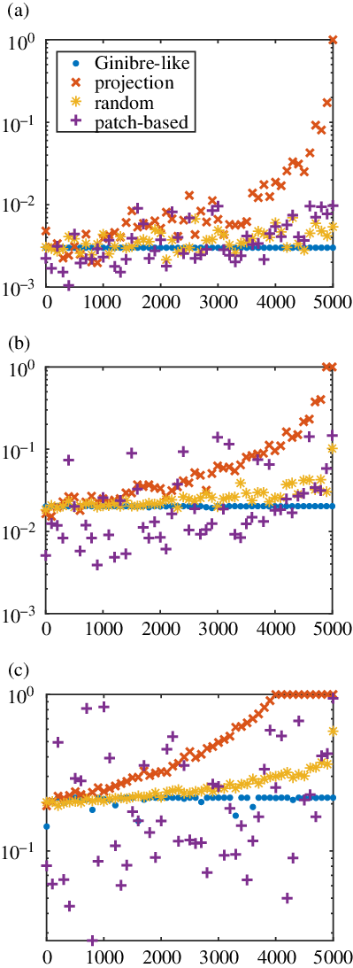
Figure 5: Behavior of the Bernoulli probabilities $q_k, \, k \in \{1,\dots, N \}$
, for the kernels presented in Section 4.1, considering a ground set of
$q_k, \, k \in \{1,\dots, N \}$
, for the kernels presented in Section 4.1, considering a ground set of $N= 5000$
elements and varying the expected cardinality of the DPP: (a)
$N= 5000$
elements and varying the expected cardinality of the DPP: (a) $\mathbb{E}(|Y|) = 15$
, (b)
$\mathbb{E}(|Y|) = 15$
, (b) $\mathbb{E}(|Y|) = 100$
, (c)
$\mathbb{E}(|Y|) = 100$
, (c) $\mathbb{E}(|Y|) = 1000$
.
$\mathbb{E}(|Y|) = 1000$
.
In order to understand more precisely to what extent high eigenvalues penalize the efficiency of the sequential thinning algorithm (Algorithm 3), Figure 6 compares its running times with that of the spectral algorithm (Algorithm 1) as a function of the eigenvalues of the kernel K. For these experiments, we consider a ground set of size $|{\mathcal{Y}}| = 5000$
items and an expected cardinality equal to 15. In the first case (a), the eigenvalues are either equal to 0 or to
$|{\mathcal{Y}}| = 5000$
items and an expected cardinality equal to 15. In the first case (a), the eigenvalues are either equal to 0 or to $\lambda_{\text{max}}$
, with m non-zero eigenvalues so that
$\lambda_{\text{max}}$
, with m non-zero eigenvalues so that $m \lambda_{\text{max}} = 15$
. It shows that above a certain
$m \lambda_{\text{max}} = 15$
. It shows that above a certain $\lambda_{\text{max}}$ $(\simeq 0.65)$
, the sequential thinning algorithm is no longer the fastest. In particular, when
$(\simeq 0.65)$
, the sequential thinning algorithm is no longer the fastest. In particular, when $\lambda_{\text{max}} = 1$
, the running time takes off. In the second case (b), the eigenvalues
$\lambda_{\text{max}} = 1$
, the running time takes off. In the second case (b), the eigenvalues $(\lambda_k)$
are randomly distributed between 0 and
$(\lambda_k)$
are randomly distributed between 0 and $\lambda_{\text{max}}$
so that
$\lambda_{\text{max}}$
so that $\sum_k \lambda_k = 15$
. In practice,
$\sum_k \lambda_k = 15$
. In practice, $(N-1)$
eigenvalues are exponentially distributed, with expectation
$(N-1)$
eigenvalues are exponentially distributed, with expectation ${{(15- \lambda_{\text{max}})}/{(N-1)}}$
, and the last eigenvalue is set to
${{(15- \lambda_{\text{max}})}/{(N-1)}}$
, and the last eigenvalue is set to $\lambda_{\text{max}}$
. In this case the sequential thinning algorithm remains faster than the spectral algorithm, even with high values of
$\lambda_{\text{max}}$
. In this case the sequential thinning algorithm remains faster than the spectral algorithm, even with high values of $\lambda_{\text{max}}$
, except when
$\lambda_{\text{max}}$
, except when $\lambda_{\text{max}} = 1$
. This can be explained by the fact that, by construction of this kernel, most of the eigenvalues are very small. The average size of the Bernoulli process generated (light grey, right axes) also illustrates the influence of the eigenvalues.
$\lambda_{\text{max}} = 1$
. This can be explained by the fact that, by construction of this kernel, most of the eigenvalues are very small. The average size of the Bernoulli process generated (light grey, right axes) also illustrates the influence of the eigenvalues.
Table 1 presents the individual weight of the main steps of the three algorithms. Concerning the sequential algorithm, logically, the matrix inversion is the heaviest part taking $74.25\%$
of the global running time. These proportions remain the same when the expected number of points n grows. The main operation of the spectral algorithm is by far the eigendecomposition of the matrix K, counting for 83% of the global running time, when the expectation of the number of points to sample evolves with the size of
$74.25\%$
of the global running time. These proportions remain the same when the expected number of points n grows. The main operation of the spectral algorithm is by far the eigendecomposition of the matrix K, counting for 83% of the global running time, when the expectation of the number of points to sample evolves with the size of ${\mathcal{Y}}$
. Finally, the sequential sampling is the heaviest step of the sequential thinning algorithm. We have already mentioned that the thinning is very fast and that it produces a point process with cardinality as close as possible to the final DPP. When the expected cardinality is low, the number of selected points by the thinning process is low too, so the sequential sampling part remains bounded (
${\mathcal{Y}}$
. Finally, the sequential sampling is the heaviest step of the sequential thinning algorithm. We have already mentioned that the thinning is very fast and that it produces a point process with cardinality as close as possible to the final DPP. When the expected cardinality is low, the number of selected points by the thinning process is low too, so the sequential sampling part remains bounded ( $86.53 \%$
when the expected cardinality
$86.53 \%$
when the expected cardinality $\mathbb{E}(|Y|)$
is constant). On the contrary, when
$\mathbb{E}(|Y|)$
is constant). On the contrary, when $\mathbb{E}(|Y|)$
grows, the number of points selected by the dominated process rises as well so the running time of this step is growing (with a mean of
$\mathbb{E}(|Y|)$
grows, the number of points selected by the dominated process rises as well so the running time of this step is growing (with a mean of $89.39\%$
). As seen before, the global running time of the sequential thinning algorithm really depends on how good the domination is.
$89.39\%$
). As seen before, the global running time of the sequential thinning algorithm really depends on how good the domination is.
Table 1: Detailed running times of the sequential, spectral, and sequential thinning algorithms for varying ground sets ${\mathcal{Y}}$
with
${\mathcal{Y}}$
with $|{\mathcal{Y}}| \in [100,5000]$
using a patch-based kernel.
$|{\mathcal{Y}}| \in [100,5000]$
using a patch-based kernel.
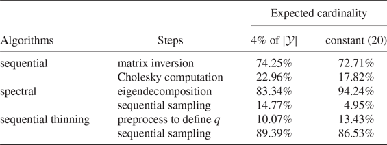
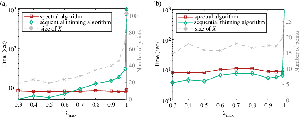
Figure 6: Running times of the spectral and sequential thinning algorithms (Algorithms 1 and 3) as a function of $\lambda_{\text{max}}$
: (a) m eigenvalues equal to
$\lambda_{\text{max}}$
: (a) m eigenvalues equal to $\lambda_{\text{max}}$
and
$\lambda_{\text{max}}$
and $N-m$
zero eigenvalues, (b) N random eigenvalues between 0 and
$N-m$
zero eigenvalues, (b) N random eigenvalues between 0 and $\lambda_{\text{max}}$
. The size of the Bernoulli process X is also displayed in light grey (right axis). Here
$\lambda_{\text{max}}$
. The size of the Bernoulli process X is also displayed in light grey (right axis). Here $|{\mathcal{Y}}| = 5000$
and
$|{\mathcal{Y}}| = 5000$
and $\mathbb{E}(|Y|) = 15$
.
$\mathbb{E}(|Y|) = 15$
.
Thus the main case when this sequential thinning algorithm (Algorithm 3) fails to compete with the spectral algorithm (Algorithm 1) is when the eigenvalues of the kernel are equal or very close to 1. This algorithm improves the sampling running times when the target size of the sample is very low (below 25 in our experiments).
In cases when multiple samples of the same DPP have to be drawn, the eigendecomposition of K can be stored and the spectral algorithm is more efficient than ours. Indeed, in our case the computation of the Bernoulli probabilities can also be saved, but the sequential sampling is the heaviest task and needs to be done for each sample.
4.3. Sampling the patches of an image
A random and diverse subselection of the set of patches of an image can be useful for numerous image processing applications. A first obvious one is image compression. Indeed, it is possible to obtain a good reconstruction of the image from a very small portion of its patches. It is sometimes necessary to keep only the most informative patches of the image, if possible a small amount, and reconstruct the image and store it, using only these few patches. Moreover, most patch-based algorithms could use such a subselection of patches to improve or at least speed up its procedures, e.g. for denoising [Reference Buades, Coll and Morel11]. To do this, the selected patches must be representative of the patches’ diversity, and this is what DPPs offer. Launay and Leclaire [Reference Launay and Leclaire30] explore this strategy to speed up a texture synthesis algorithm.
Given an image u and a set $\mathcal{P}$
of
$\mathcal{P}$
of $10\,000$
randomly picked patches of u, we compare the selection strategies using either a DPP or a random uniform selection. Let us recall the patch-based kernel (c) defined as the L-ensemble associated with
$10\,000$
randomly picked patches of u, we compare the selection strategies using either a DPP or a random uniform selection. Let us recall the patch-based kernel (c) defined as the L-ensemble associated with
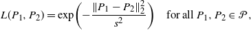 \begin{equation*}L(P_1,P_2) = \exp\biggl( -\frac{\|P_1-P_2\|_2^2}{s^2}\biggr)\quad {\text{for all } P_1, P_2 \in \mathcal{P},}\end{equation*}
that is, L is a Gaussian kernel applied to the Euclidean distance between the patches of $\mathcal{P}$
. This function is commonly chosen to define a similarity measure between patches. It is relevant since in general the reconstruction error is computed as a function of the Euclidean distance between the original image and the reconstructed image. We set the bandwidth or scale parameter s to be proportional to the median of the interdistances between the patches, as advised by Aggarwal [Reference Aggarwal2] and Tremblay, Barthelmé, and Amblard [Reference Tremblay, Barthelmé and Amblard44].
$\mathcal{P}$
. This function is commonly chosen to define a similarity measure between patches. It is relevant since in general the reconstruction error is computed as a function of the Euclidean distance between the original image and the reconstructed image. We set the bandwidth or scale parameter s to be proportional to the median of the interdistances between the patches, as advised by Aggarwal [Reference Aggarwal2] and Tremblay, Barthelmé, and Amblard [Reference Tremblay, Barthelmé and Amblard44].
Figures 7 and 8 present several reconstructions of two images, obtained by uniform selection or by the DPP defined above, with various expected sample sizes. Note that while we can control the exact cardinality of the uniform selections, the number of patches in the DPP selections varies, as we can only control the expected cardinality during the sampling process. These figures show how a selection from a DPP provides better reconstructions than a uniform selection, especially when the number of patches is low. Indeed, as the DPP sampling favors a diverse set of patches, it is less likely to miss an essential information of the image. On the contrary, nothing prevents the uniform selection from selecting very similar patches. The pool image in Figure 8, for cardinality equal to 5, clearly illustrates this. The number of patches in an image depends on the size of the image and is often higher than $10\,000$
, while the selection needs to be small (between 5 and 100): here the use of our sequential thinning algorithm is pertinent.
$10\,000$
, while the selection needs to be small (between 5 and 100): here the use of our sequential thinning algorithm is pertinent.
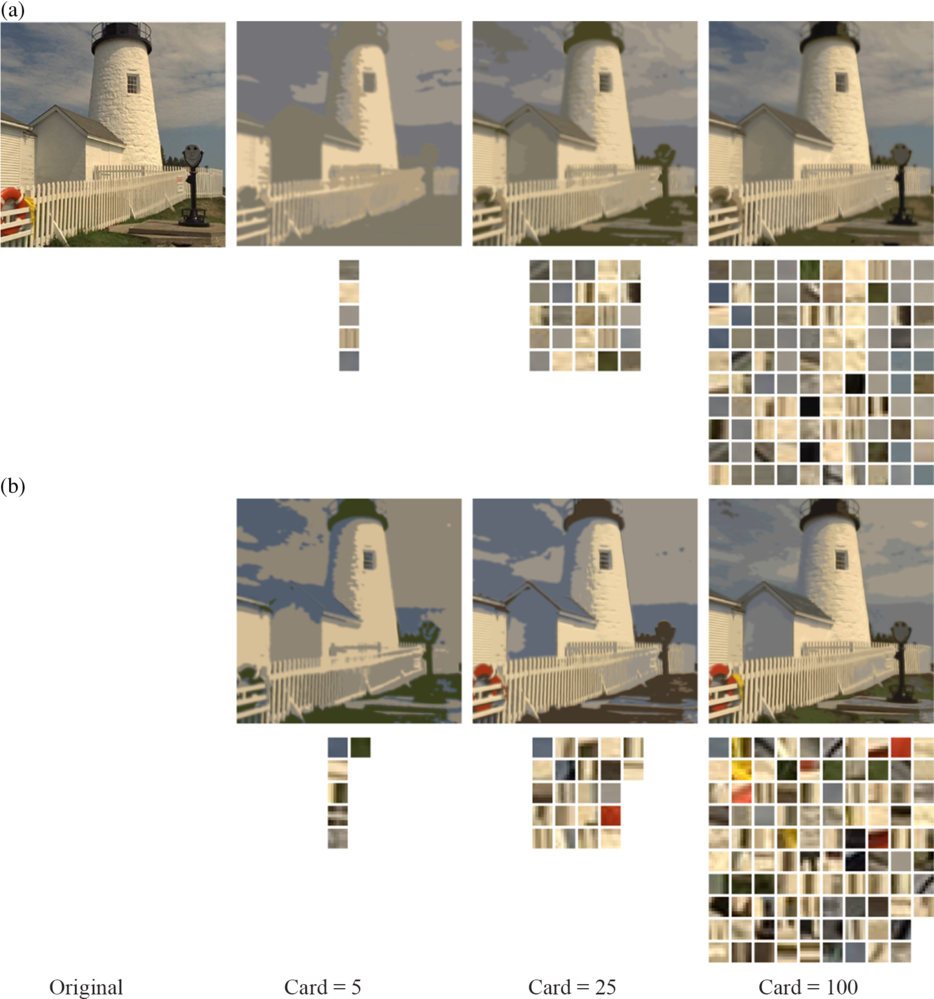
Figure 7: Reconstruction of lighthouse image. (a) Original and reconstructions with uniformly sampled patches and below, the corresponding selected patches. (b) Reconstructions with patches sampled according to a DPP and below, the corresponding selected patches.
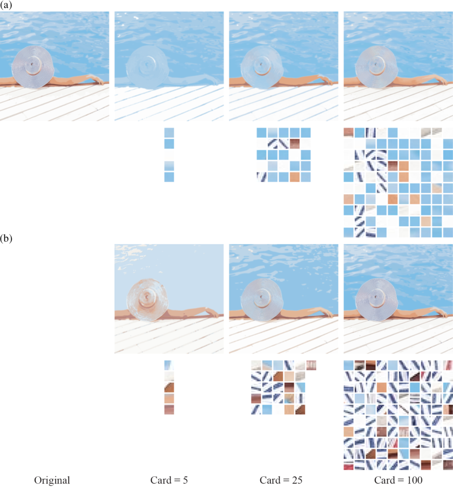
Figure 8: Reconstruction of pool image. (a) Original and reconstructions with uniformly sampled patches and below, the corresponding selected patches. (b) Reconstructions with patches sampled according to a DPP and below, the corresponding selected patches.
5. Discussion
In this paper we have proposed a new sampling algorithm (Algorithm 3) adapted to general determinantal point processes, which does not use the spectral decomposition of the kernel and which is exact. It proceeds in two phases. The first one samples a Bernoulli process whose distribution is adapted to the targeted DPP. It is a fast and efficient step that reduces the initial number of points of the ground set. We know that if $I-K$
is invertible, the expectation of the cardinality of the Bernoulli process is proportional to the expectation of the cardinality of the DPP. The second phase is a sequential sampling from the points selected in the first step. This phase is made possible by the explicit formulations of the general marginals and the pointwise conditional probabilities of any DPP from its kernel K. The sampling is sped up using updated Cholesky decompositions to compute the conditional probabilities. MATLAB® and Python implementations of the sequential thinning algorithm can be found online (https://www.math-info.univ-paris5.fr/~claunay/exact_sampling.html).
$I-K$
is invertible, the expectation of the cardinality of the Bernoulli process is proportional to the expectation of the cardinality of the DPP. The second phase is a sequential sampling from the points selected in the first step. This phase is made possible by the explicit formulations of the general marginals and the pointwise conditional probabilities of any DPP from its kernel K. The sampling is sped up using updated Cholesky decompositions to compute the conditional probabilities. MATLAB® and Python implementations of the sequential thinning algorithm can be found online (https://www.math-info.univ-paris5.fr/~claunay/exact_sampling.html).
In terms of running times, we have detailed the cases for which this algorithm is competitive with the spectral algorithm, in particular when the size of the ground set is high and the expected cardinality of the DPP is modest. This framework is common in machine learning applications. Indeed, DPPs are an interesting solution to subsampling a data set, initializing a segmentation algorithm, or summarizing an image, examples where the number of data points needs to be significantly reduced.
Appendix A. Möbius inversion formula
Proposition A.5. (Möbius inversion formula.) Let V be a finite subset and let f and g be two functions defined on the power set $\mathcal{P}(V)$
of subsets of V. Then
$\mathcal{P}(V)$
of subsets of V. Then
 \begin{equation*}{\textit{for all }} A\subset V,\quad f(A) = \sum_{B\subset A} (-1)^{|A\setminus B|} g(B)\quad\Longleftrightarrow\quad{\textit{for all }} A\subset V,\quad g(A) = \sum_{B\subset A} f(B),\end{equation*}
and
 \begin{equation*}{\textit{for all }} A\subset V,\quad f(A) = \sum_{B\supset A} (-1)^{|B\setminus A|} g(B)\quad\Longleftrightarrow\quad{\textit{for all }} A\subset V,\quad g(A) = \sum_{B\supset A} f(B).\end{equation*}
Proof. The first equivalence is proved in [Reference Mumford and Desolneux35], for example. The second equivalence corresponds to the first applied to $\widetilde{f}(A) = f(\overline{A})$
and
$\widetilde{f}(A) = f(\overline{A})$
and $\widetilde{g}(A) = g(\overline{A})$
. You will find more details on this matter in Rota [Reference Rota39]. □
$\widetilde{g}(A) = g(\overline{A})$
. You will find more details on this matter in Rota [Reference Rota39]. □
Appendix B. Cholesky decomposition update
To be efficient, the sequential algorithm relies on Cholesky decompositions that are updated step by step to save computations. Let M be a symmetric semi-definite matrix of the form
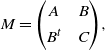 \begin{equation*}M =\begin{pmatrix}A & \quad B\\[4pt] B^t & \quad C\end{pmatrix}\!,\end{equation*}
where A and C are square matrices. We suppose that the Cholesky decomposition $T_A$
of the matrix A has already been computed and we want to compute the Cholesky decomposition
$T_A$
of the matrix A has already been computed and we want to compute the Cholesky decomposition $T_M$
of M. Then set
$T_M$
of M. Then set
 \begin{equation*}V = T_A^{-1} B \quad \text{and} \quad X = C - V^t V = C - B^t A^{-1} B {,}\end{equation*}
the Schur complement of the block A of the matrix M. Let $T_X$
denote the Cholesky decomposition of X. Then the Cholesky decomposition of M is given by
$T_X$
denote the Cholesky decomposition of X. Then the Cholesky decomposition of M is given by
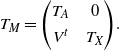 \begin{equation*}T_M =\begin{pmatrix}T_A & \quad 0\\[4pt]
V^t & \quad T_X\end{pmatrix}\!.\end{equation*}
\begin{equation*}T_M =\begin{pmatrix}T_A & \quad 0\\[4pt]
V^t & \quad T_X\end{pmatrix}\!.\end{equation*}
Indeed,
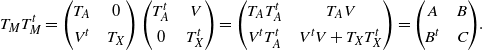 \begin{equation*}T_M T_M^t=\begin{pmatrix}T_A & \quad 0\\[4pt]
V^t & \quad T_X\end{pmatrix}\begin{pmatrix}T_A^t & \quad V\\[4pt]
0 & \quad T_X^t\end{pmatrix} =\begin{pmatrix}T_A T_A^t & \quad T_A V\\[4pt]
V^t T_A^t & \quad V^t V + T_X T_X^t\end{pmatrix}=\begin{pmatrix}A & \quad B\\[4pt]
B^t & \quad C\end{pmatrix}\!.\end{equation*}
\begin{equation*}T_M T_M^t=\begin{pmatrix}T_A & \quad 0\\[4pt]
V^t & \quad T_X\end{pmatrix}\begin{pmatrix}T_A^t & \quad V\\[4pt]
0 & \quad T_X^t\end{pmatrix} =\begin{pmatrix}T_A T_A^t & \quad T_A V\\[4pt]
V^t T_A^t & \quad V^t V + T_X T_X^t\end{pmatrix}=\begin{pmatrix}A & \quad B\\[4pt]
B^t & \quad C\end{pmatrix}\!.\end{equation*}
Acknowledgement
This work was supported by grants from Région Ile-de-France. We thank the reviewers for their valuable comments and suggestions that helped us to improve the paper.


