


Education and human capital investment are topics of longstanding interest in the economic history of Victorian and Edwardian England. The literature is particularly rich in macro-level analyses of the English educational system, with an emphasis on primary schooling and advanced technical education. David Landes, Peter Mathias, and Francois Crouzet, for example, all assess the quantity and quality of educational provision in nineteenth-century England and conclude that underinvestment was a key ingredient in Britain's growth slowdown relative to the more dynamic economies of the United States and Germany.1
Crouzet, Victorian Economy; Landes, Unbound Prometheus; and Mathias, First Industrial Nation.
Lindert, “Comparative Political Economy.”
Pollard, Britain's Prime.
Birchenough, History; Curtis, History; Hurt, Education; Sutherland, Elementary Education; West, Education and the State and Education and the Industrial Revolution.
West, Education and the Industrial Revolution, p. 42.
Given the important role that education is widely regarded to have played in the growth experiences of the nineteenth and twentieth centuries' leading economies, it is perhaps surprising how little has been done to analyze schooling at the micro-level of the individual student or household before the twentieth century. This omission is particularly striking considering the central place that education studies have come to hold in the modern labor economics literature.6
For a survey of this extensive literature, see Card, “Causal Effect.”
Mitch, “Underinvestment” and Rise.
Mitch, “Literacy.”
In this article, I use new panel data from England in the second half of the nineteenth century to perform a micro-level analysis of primary schooling. By constructing a sample of 5,337 school-aged males linked from the 1851 to the 1881 Census of the Population, I am able to observe both childhood school attendance and subsequent adult labor market outcomes for a reasonably large, nationally representative sample of individuals. With this information it is possible, for the first time, to systematically assess the return to education in nineteenth-century England for the population as a whole. I also provide an empirical analysis of the determinants of childhood primary school attendance. I find that family background exerted a large influence on the probability of attendance. For example, sons of fathers with high-class occupations were more likely to attend school, and to attend at a later age, as were sons of working mothers. The opportunity cost of foregone labor, especially within the home, was also an important consideration. As for the effect of school attendance, the results indicate that it conveyed real, substantive economic benefits to adult participants in the labor market that outweighed the total costs of childhood attendance. At the same time, the magnitude of the effect, while nontrivial, appears to have been small in two important dimensions. First, the effect of education was markedly smaller than the effect of several other important variables; father's socioeconomic status, in particular, had a significantly greater influence on adult socioeconomic status than did primary school attendance. Second, though the comparability of the results is tenuous, the measured return to primary education appears to be smaller than typical estimates of the returns to education in the modern labor and development economics literature.
PRIMARY SCHOOLING IN NINETEENTH-CENTURY ENGLAND
Long before the role of mass primary education in England's economic growth became an important topic for twentieth-century economic historians, it was a matter of great concern for contemporary thinkers and policy makers. At issue was the education gap opening up between England on the one hand and the United States and Germany on the other. England was decades behind the United States in the establishment of a national system of primary education, and even further behind in achieving high rates of school attendance and literacy. The gap relative to Germany was greater. Prussia established compulsory education in 1763, more than a century before England. By 1860, 97.5 percent of all German children between the ages of 6 and 14 attended school; in England, only half of 6–14 year olds were in school in 1851.9
The German figure is from Crouzet, Victorian Economy, p. 415. The British figure is calculated from the 2 percent sample of the 1851 census. The lag persisted into the twentieth century; see Easterlin, “Why Isn't the Whole World,” p. 18.
For a concise summary of this complex issue, see Sutherland, Elementary Education.
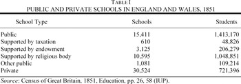
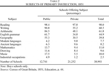
Even in the national educational systems of today, quality varies across schools; in Victorian England's informal system, the variation was tremendous. Public schools, which received a portion of their income from a source other than student fees and were subject to oversight from funding bodies, varied less than did private schools. Because of their endowments, public schools cost less to attend and spent on average 48 percent more per student than did private schools.11
Mitch, Rise, p. 144.
Attending school was not necessarily easy or cheap. Availability varied greatly, particularly between rural and urban areas; a school was more likely to be nearby in populous Lancashire (2.5 schools per 1,000 acres) than in rural Northumberland (0.5 per 1,000 acres), for example. In a time before motor vehicles, a distance of several miles could have precluded school attendance. At the same time, urban areas tended to have fewer schools relative to population size, so a spot in a reasonably sized class was not guaranteed even if a school was nearby. Cost was another barrier to school attendance.12
The following wage and school fee information are from ibid., chap. 7 and pp. 202–04.
At precisely which ages and for how long children went to school is not known exactly. The censuses reveal which children were in school, but they give no information on enrollment prior to enumeration. Figure 1 shows the age/attendance profile at mid-century according to the 1851 census. Probability of attendance peaks at age eight and declines steeply after age 11. Taking the area under the attendance probability curve indicates that the average child would be in school for approximately five years, though of course these might not be complete years. The Newcastle Commission also found that the majority of students were enrolled from the ages of 6 to 10, though a substantial minority began at five and many remained until 12.13
West, Education and the Industrial Revolution, p. 82.
Newcastle Report, pp. 234–35.
Ibid., p. 245.
Ibid., p. 238.
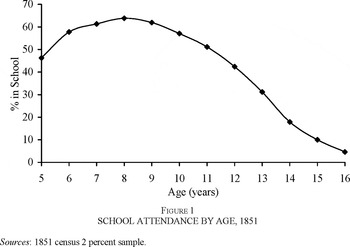
Figure 1 SCHOOL ATTENDANCE BY AGE, 1851
ANALYZING SCHOOLING WITH LINKED CENSUS DATA
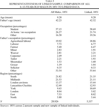
In order to estimate the return to education, it is necessary to observe individuals' schooling and labor market outcomes. A new data set of 5,337 school-aged males linked from the 1851 to the 1881 population censuses provides the longitudinal information to observe the schooling outcomes of children and their subsequent adult labor market outcomes. Individuals between the ages of 6 and 13 in 1851 are nominally linked between the two censuses by first and last name and parish and year of birth—responses which should be constant across censuses. Two sources are used to perform the linkage: a computerized 2 percent sample of the 1851 census and a computerized version of the complete count 1881 census.17
Both datasets are available from the U.K. Data Archive, as studies number 1316 and 4177, respectively.
For more detail on the sources and techniques of the census linkage procedure, including the matching algorithm, potential sources of bias, and expected versus actual linkage success rate, see Long, “Rural-Urban Migration.”
The two central pieces of information from the data are schooling in 1851 and labor market outcome in 1881. Both are reported in the occupation field of the censuses. Parents were to record their children as “scholars” if they were receiving formal education. Of all the Victorian censuses, the 1851 enumerators' instructions were the clearest and most specific, and as a result, the information on school attendance from that year is more useful than from any other in the nineteenth-century. In 1851, parents were to report their children as scholars if they were older than five and were “daily attending school, or receiving regular tuition under a master or governess at home.” Unlike later definitions, it excluded children taught by a parent and, critically, those whose only education came from Sunday schools, allowing attention to be restricted to children receiving a regular elementary education. The instructions were not followed faultlessly, and the pool of scholars even from 1851 represents an imperfect record.19
Higgs, Clearer Sense.
Altogether, the population census shows 2,046,848 scholars present in England and Wales in 1851. Independent confirmation of the census record's reliability is provided by the separate Education Census of 1851, which involved delivering questionnaires to approximately 70,000 heads of schools. This source gives a very similar result: 2,144,378 scholars in day schools (1851 Census, Education, pp. xxviii, xiv).
The 1851 record offers another advantage. As compulsory primary schooling did not become law until 1870, the incentive to report children as scholars falsely would have been far smaller before 1870 than after. In fact, the voluntary nature of elementary education in Great Britain before 1870 is central to the question at hand. Educating their children was a choice that parents faced; sending them to work, or having them work in the home, was a viable alternative. This study provides an analysis of the impact of that choice on the child's socioeconomic status 30 years later, as an adult. Therefore, the analysis is limited to boys of the prime school ages of 6 to 13.21
Girls are not included because, due to name changes at marriage, they are much more difficult to link across censuses.
Given the somewhat arbitrary nature of these age cutoffs, it is important to note that the empirical results are not sensitive to their alteration. Changing the minimum age to five or the maximum age to 12 or 14 does not appreciably change the nature of the results.
The main limitation of the schooling information available from the 1851 census is that it tells us little about the duration of schooling for an individual. Only the fact of attendance at the point of enumeration in 1851 is known; nothing is known about attendance before or after that date. The only available clue as to the duration of schooling is age in 1851. It is reasonable to assume that older boys, say those ten years old or older, who were in school in 1851 likely received an amount of schooling which could be considered large or above average relative to those out of school in 1851. They would have been far more likely to have reached the top class, progressing beyond simple reading to more complex reading, writing, simple math, and basic geography. As discussed previously, reaching the top class was generally assumed to occur sometime after age ten. The inability to observe schooling duration in the data has important implications for measuring the treatment effect of education and is discussed in greater detail in what follows.
It is not possible to estimate the effect of education on annual earnings directly, as modern studies do, because the census does not include any quantitative information on earnings. It does include detailed occupational information, which is used to construct two labor market outcome measures. The first and most direct is a ranked index of occupational class or socioeconomic status: 1–Professional, 2–Intermediate, 3–Skilled, 4–Semiskilled, and 5–Unskilled.23
This scheme was developed and has been described in detail by Armstrong and has become standard for classifying nineteenth-century British occupations. Some typical occupations are Class 1–solicitor, accountant; Class 2–farmer, carpenter (employer); Class 3–carpenter (not employer), butcher (not employer), skilled in manufacturing; Class 4–agricultural laborer, wool comber; Class 5–general laborer, porter. See Armstrong, “Use.”
To augment the results derived from the socioeconomic status measure, a second labor market outcome variable is constructed: annual nominal earnings, imputed by occupation. This measure has the advantages of being quantitative and less coarse than the occupational class measure; however, it is subject to its own substantial limitations and so should be seen as a secondary measure used to support the primary results derived using occupational class. Jeffrey Williamson provides average yearly earnings for 21 common groups of occupations in both 1851 and 1881, reproduced here in Appendix 1.24
Williamson, “Earnings Inequality” and “Structure.” Williamson discusses his sources in detail in the articles. To summarize, he uses Bowley and Wood's articles in the Journal of the Royal Statistical Society and unpublished Board of Trade data to compile wage series for agriculture, industry, mining, and construction. For the service sector, he uses records of government pay from the “Annual Estimates” reported in the House of Commons Parliamentary Papers and various sources from the private sector such as clergy lists and records of teachers' pay. These earnings figures are largely consistent with Armstrong's classification scheme. The only exception is the “Messengers and Porters” category, which is Class 5 under Armstrong's scheme but highly paid according to Williamson's data. However, there are few messengers or porters in the data, and eliminating them does not change any of the results.
Attending school in 1851 increases the probability of holding a “commercial occupation” from 7.2 percent to 8.5 percent (s.e. = 0.007), controlling for other relevant factors. School attendance is not associated with becoming a farmer.
Results are also reported leaving out the self-employed, using only occupations covered by Williamson's wage table.
A final feature of the data is worth noting. Because of the nature of the census enumeration, every person in each linked individual's household in 1851 and in 1881 is observed. This provides a great deal of useful information, particularly from 1851. Father's occupational class; mother's labor market status; number, gender, and age of siblings; and the presence of servants can all be correlated with the probability of school attendance. The single most useful piece of information is father's occupation in 1851. The nineteenth-century English labor market exhibited substantial intergenerational occupational continuity. In the sample of matched males, 40 percent of all men between the ages of 30 and 50 in 1881 were in the same occupational class as their fathers had been in 1851. The most important control variable in the analysis of the return to elementary education is father's occupational class. Class and school attendance are highly correlated; if father's class were not controlled for, some of the estimated influence of schooling on adult occupational class would be spurious, driven by the unobserved intergenerational transmission of occupation. Controlling for father's class, it is possible to measure the extent to which school attendance allowed sons to overcome poor initial prospects and realize upward intergenerational occupational mobility.27
From an econometric standpoint, the effect of father's class on schooling will decrease the precision with which the effect of each variable is measured, but it will not bias either estimate as long as neither variable is correlated with the error terms in equation 1 and equation 2.
CORRELATES OF SCHOOL ENROLLMENT
Table 4 summarizes the data. It shows results comparing those attending school in 1851 and those either at home or working. There are more students in the sample (3,130) than there are nonstudents (2,207). The group of scholars clearly differs from the group of nonscholars. In order to observe the partial effect of each potential correlate, a probit equation of school attendance probability is estimated, with results reported in Table 5. The estimation is carried out for all the boys in the sample and separately for the boys aged 6–9 and the boys aged 10–13 in 1851. Boys aged 10–13 and in school are likely to have received a more advanced elementary education, with more years of schooling and a higher likelihood of achieving the qualifications of the top class. As expected, sons of higher-class fathers were more likely to attend school than were sons from lower socioeconomic backgrounds.28
The only exception to this pattern is that sons of class 3 and class 4 fathers had no statistically significant difference in their attendance probabilities.
The χ2 statistic testing differential effect of class by age is significant at the one percent level.
These industry variables are highly correlated with the region dummies; for example, there were virtually no agricultural jobs in London, and the jobs in textiles were concentrated in Lancashire, Cheshire, and Yorkshire. Still, all of the industry effects are robust to the exclusion of the regional dummies, and the region effects are robust to the exclusion of the industry dummies.
In this Scotland is an interesting case, and with the newly available manuscript-level information from the 1881 Census of the Population of Scotland it will be the subject of future work.
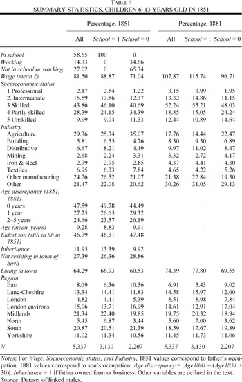
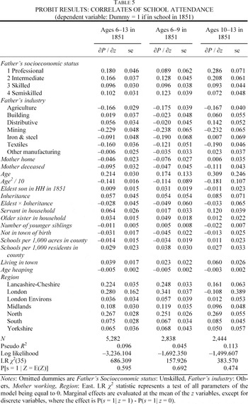
Several variables were included to incorporate the opportunity cost of sending a child to school. School availability is proxied for by including the number of schools per thousand residents in the county, the number of schools per thousand acres (intended to capture distance), and a variable indicating whether the family lived in a town of 2,500 or more residents. The two school density variables did not have a statistically significant effect, perhaps because they ignore important intracounty variation in school density. On the other hand, living in an urban area increased the probability of enrollment by four percentage points, reflecting the greater availability of schools in more populated areas. Household demographics also played a role in the schooling decision. Households in which the mother worked at a wage-earning job were more likely to send their sons to school than were households in which the mother stayed at home or was deceased. Quite likely, working mother families could better afford the opportunity cost of foregone child wages, whereas families headed by a widower could least afford to do without the son's wages or home production. If child-minding were the primary motivation for schooling, then widower-headed households would have been more likely to send their sons to school; instead, they were the least likely. The presence of at least one servant in the household increased the likelihood that a son would be schooled, as did the son having an older sister in the household. The presence of younger siblings was negatively correlated with school enrollment. All three factors point to the value of sons' household labor and its importance in the schooling decision. Younger siblings could require looking after, potentially keeping a son out of school; on the other hand, a servant or older sister might be called upon instead to perform this or other household chores, freeing up sons to attend school.
RETURN TO SCHOOLING
Time spent in elementary school as a child should have conferred at least two distinct advantages to an adult participating in the Victorian labor market. First was the acquisition of general human capital. Literacy was perhaps the most important skill learned in elementary school. According to Mitch less than half of the male English labor force in 1851 worked in jobs for which literacy was “unlikely to be useful.”32
Mitch, Rise, table 2.1.
Ibid., p. 13.
One would expect to find, then, a positive relationship between school attendance and occupational class or annual earnings. However, parents did not simply face a one-time choice of sending a child to school or not; they would have made the decision year by year, or even month by month. The ideal variable for measuring the educational outcome of each individual would be duration of schooling. Unfortunately, as discussed previously, this information cannot directly be observed from the census. There are several potential strategies for incorporating the available age and attendance information into a rough estimate of school duration. The simplest approach, and the one emphasized here, is to treat schooling as a dichotomous variable, which is how it appears in the data. The school variable can be made to account for likely differences in school duration across individuals in a crude manner by splitting the sample into younger and older boys. The dichotomous school variable is then interpreted differently for the two age groups. For the older group (here, ages 10–13) those observed to be in school in 1851 are assumed to have received an advanced elementary education—attaining or nearly attaining the qualifications of a first-level student—whereas those observed to be out of school are assumed not to have. For the younger group (ages 6–9), those in school are assumed to have received at least some elementary schooling, while those not in school in these prime ages are more likely to have received little or no schooling. This method will inevitably result in some misspecification. Some individuals out of school in 1851 may still have received an average or above average course of schooling at some point in their childhood, and some in school in 1851 may have attended for only a year or even less. To make some effort to account for this, a second schooling measure is developed that uses father's class and the school attendance of siblings (two observable variables that are highly predictive of attendance) to estimate total schooling duration for each individual. The derivation of this estimate is described in Appendix 2. Essentially, it attributes some years of schooling to individuals not in school in 1851 who were nevertheless likely to have received some unobserved schooling, where likelihood of unobserved schooling is determined by father's class and the presence in the household of siblings in school. However, because of the very strong assumptions needed to construct these estimates, they should be seen as secondary, supporting results. Splitting the sample by age lessens the misspecification of the dichotomous variable approach to an extent, and in the end, this approach is in line with the sparse information available in the data.
EFFECT OF SCHOOLING ON OCCUPATIONAL CLASS
The primary labor market outcome variable used here is occupational class in 1881. Occupational class is a discrete, qualitative variable with five ranked categories, which suggests ordered probit analysis. Table 6 shows the results of estimating the following equation by ordered probit maximum likelihood

where yi is the individual's occupational class in 1881, c ∈ [1,2,3,4,5], si = 1 if the individual was in school in 1851 and 0 otherwise, fathersclassi is a set of dummy variables capturing father's occupational class in 1851, xi,1851 is a vector of additional controls, and β1 measures the treatment effect of schooling. The equation is estimated for the whole sample and separately for boys aged 6–9 in 1851 and 10–13 in 1851.
34This specification assumes a constant effect of school attendance across different class backgrounds. To examine the possibility of variable school effects by class, equation 1 was reestimated with a full set of dummy variables interacting school and father's class. The four school-class dummies were jointly statistically insignificant for each of the three age groups: 6–13, 6–9, and 10–13. The χ2 test statistics were, respectively, 1.72, 2.27, and 6.77.
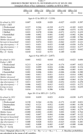
Interpreting ordered probit coefficients is not straightforward; Table 6 reveals the sign and statistical significance of the effect of each variable, and it can be used to compare the relative magnitude of different coefficients, but it does not provide a meaningful interpretation of the marginal effect of each variable. For this, it is necessary to use the results from estimating equation 1 to calculate the marginal effect of each variable on the probability of attaining the various occupational classes; these marginal effects are displayed in Table 7, along with the baseline probabilities of attaining each occupational class. Table 6 shows that, even subject to the misspecification error in the schooling variable discussed previously, the treatment effect of schooling is positive and statistically significant for all three estimation samples. As expected, the effect is greater, in fact almost twice as great, on the sample of older boys than on the sample of younger boys.35
The χ2 statistic testing differential effect of school by age is significant at the 10 percent level.
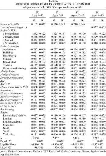
Childhood schooling, therefore, had a statistically and economically significant positive effect on adult occupational class. Still, even for the older boys, there is an important sense in which the real magnitude of that effect was small. This is most evident in comparing the magnitude of the effect of schooling with the magnitude of the effect of father's class. The effect of having a class 3 father versus a class 5 father is more than two and a half times greater than the effect of going to school in 1851 versus not going to school (0.432 versus 0.162), the effect of a class 2 father (0.534) is more than three times greater, and the effect of a class 1 father (1.432) is almost nine times greater.36
Each of these differences in coefficients is statistically significant at the 1 percent level.
For a detailed analysis of the low level of intergenerational mobility in England relative to the U.S., see Long and Ferrie, “Tale.”
As before, the differences in coefficients are significant at the 1 percent level for classes 1 and 2; however, for class 3 the difference is no longer statistically significant.
Another comparison also demonstrates the small relative magnitude of the schooling effect: the effect of numeracy was significantly greater than the effect of schooling. Numeracy, in other words basic quantitative ability, is not directly observable, but the structure of the linked census data provides a proxy: age discrepancy, defined as |Reported; Age1881 – (Reported; Age1851 + 30)|.39
In most cases for this sample, the parents would have reported the age in 1851. It could be possible, therefore, for an individual to report his correct age and still have a non-zero value of age discrepancy, if his parents had incorrectly reported his age in 1851. This seems unlikely, though, as most people would have learned their age from their parents.
Only the difference for the whole sample is statistically significant (at the 5 percent level).
ROBUSTNESS CHECK: EFFECT OF SCHOOLING ON EARNINGS
To check the robustness of the preceding results, a new equation is estimated to measure the effect of childhood school attendance on adult annual earnings
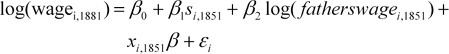
β1 still captures the treatment effect of education, now expressed as the percent effect of school attendance on adult earnings. Table 8 shows the results of estimating equation 2 by ordinary least squares. Attending school in 1851 increased adult earnings by 7.7 percent for the whole sample and by 10.7 percent for the 10–13 year olds receiving advanced elementary education. As before, these are statistically and economically significant effects.
41Re-estimating equation 2 on only those individuals who can be assigned a wage directly from Williamson's wage table (in other words dropping the self-employed) yields slightly smaller estimates: β1 = 0.0675 (s.e. = 0.0153) for the whole sample, and β1 = 0.0956 (s.e. = 0.023) for the 10–13 year olds.
Mitch, Rise.
This result would not hold for all workers. The average 1851 wage for class 4 and 5 workers was only £35.7 per year. The resulting schooling premium of £2.75 per year would not be enough to compensate for the cost of schooling with a high discount rate of 0.20. The cost-benefit analysis for low-class workers hinges on the assumed discount rate; with a discount rate as high as 0.13, 20 work years is enough to compensate a low-class worker for the cost of schooling.
The nature of the data used here is very different from the data typically used to measure the return to education in the modern labor and development economics literature, so a direct comparison of results is impossible. There are at least two sources of downward bias in the estimates presented above: the misspecification inherent in the dichotomous schooling variable and the use of earnings imputed by occupation. Using imputed rather than observed earnings means that only between-occupation wage variation is measured. Any effect of education on earnings within occupations is unobserved. Still, the modern estimates give some sense of context for the current results. Typical empirical studies in the United States and United Kingdom have found that each year of secondary education increases annual earnings by somewhere between 5 and 15 percent.44
See for example Card, “Causal Effect”; and Harmon and Walker, “Estimates.”
Goldin and Katz, “Education.”
Schultz, “Evidence.”
Goldin and Katz, “Education.”
The difficulty in comparing the results for England to other studies is exacerbated by not knowing how many additional years of schooling the 10–13 year old students received on average. If they typically received more than three years of additional education, this would imply a lower per-year rate of return and would increase the difference in results.
CONCLUDING REMARKS
This article adds a micro-level analysis of school attendance and the return to education to a large literature on the history of primary schooling in Victorian England. In a regime of voluntary elementary education that was at most partly subsidized, households responded predictably in their schooling decisions. Sons of fathers with high-class occupations were much more likely to be in school in 1851, and to be in school at later ages, than were sons of lower-class fathers. Not surprisingly, opportunity costs mattered. In urban areas, where schools were more readily available, probability of attendance was greater. In households where sons' domestic labor was likely to be more valuable due to the presence of younger siblings or the absence of an elder sister, probability of attendance was lower. The outcomes of these schooling decisions had long-lasting effects. Childhood school attendance was positively associated with the attainment of higher class, higher paying adult occupations. This was especially true for boys in school over the age of ten, who likely received more advanced elementary education. For example, schooling increased the odds for this group of attaining a relatively high-paying class 2 occupation from 14 to 17 percent, and it decreased the odds of a low-paying class 4 or 5 job from 29 to 22 percent. For most workers, under reasonable assumptions of time preference, the corresponding wage gains would have more than offset the cost of schooling.
However, although childhood schooling did then pay off, there is still an important sense in which the return to schooling looks small. First and most importantly, father's occupational class exerted a much greater influence on own adult class than did school attendance. This result holds even for the older children receiving more advanced schooling. Second, the impact of school attendance on adult earnings appears to be small relative to other estimates of the return to education for developed and developing countries today and for the United States early in the twentieth century. This result is highly tentative; the data and methods used here are too different from those used elsewhere to make any direct comparisons. Still, these results taken together do provide some very preliminary evidence for a low return to primary schooling in Victorian England. This could be interpreted as evidence that England's schools were, on average, low quality, or at least that the human capital they provided was not of great economic value. Alternately, it could be interpreted as a statement about England's labor market, that a high level of intergenerational occupational stasis minimized the economic value of primary schooling. Either way, the conclusion remains that primary schooling, while conveying measurable socioeconomic gains, was a limited path to mobility in Victorian England.
Appendix 1
Appendix 2: Estimating Schooling Duration
Given information on age, family characteristics, and school attendance at one point in time for each individual, the goal is to find E(di | si, ai, zi), where di is total duration of schooling, si is a dummy variable indicating whether an individual is observed to be in school in 1851, ai is age, and zi is a vector of relevant family demographic variables. Strong assumptions on attendance patterns are necessary. First, I assume that all individuals who receive any elementary schooling began their schooling at age six and that none remain in elementary school past the age of 13. This reflects general attendance patterns according to sources such as the Newcastle Commission and is in keeping with the very low attendance rates past the age of 13. Still, given the often haphazard nature of nineteenth-century primary school attendance, these are strong assumptions. Fortunately, the estimates are robust to changing the assumed starting and ending ages. The final assumption is that primary school enrollment was continuous: students who left school did not return. Again, under the informal English school system, this certainly would not have held in all cases. Even so, it is a necessary and reasonable simplifying assumption.
Given these assumptions, it is possible to recover the hazard rate of school exit for each age and to use these hazard rates to calculate the conditional expected school duration for each individual. First, let p6 be the probability of attending school at age six, observable in the data as the proportion of six year olds in school in 1851. Next, note that the probability of attending school at age a > 6 is
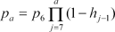
where ha is the hazard rate of school exit at age a, that is, the probability of leaving school after age a conditional on having attended through age a. From this it follows that

. Because pa is observable for each age as the proportion of individuals of that age in school, each of the hazard rates h6, h7, …, h14 can be recovered. In addition, different hazard rates can be calculated for individuals with different background characteristics. To construct the hazard rates for this analysis, I incorporated two variables that are highly correlated with school attendance: father's socioeconomic status and the school attendance of siblings. With the hazard rates in hand, the conditional expectation of total school duration d for an individual of age a and background characteristics z observed to be in school in 1851 is
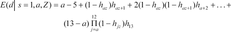
where h13 is assumed to be 1. (a – 5) is the known completed school duration, and the summation that follows is the conditional expected duration of additional schooling continuing past age a. For individuals of age a observed to be out of school, the conditional expectation of total school duration is
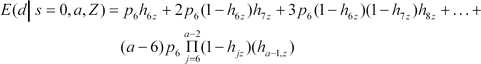
and ha – 1 = 1 because s = 0.
This article is based on the second chapter of my Ph.D. dissertation, Labor Mobility in Victorian Britain, Northwestern University. I am grateful to my dissertation advisors, Joel Mokyr, Joseph Ferrie, and Joseph Altonji for their many helpful comments. I received valuable input from David Green, Timothy Leunig, Susan Carter, Jane Humphries, David Mitch, Chris Taber, three anonymous referees and the editor of this Journal, and from presentations at the University of British Columbia, the University of Oxford, the 2004 Economic History Association meeting, and the 2004 Social Science History Association meeting. This research was supported by a Pew Younger Scholars Program Fellowship.


