


1. Introduction
Extensive studies of aerofoils undergoing sinusoidal pitch motions have been carried out by aeroelasticians and dynamic-stall researchers, specially aiming for flow conditions of helicopter rotor flight (Carta Reference Carta1979). However, a renewed interest in unsteady low-Reynolds-number aerodynamics has emerged due to applications in small and micro unmanned aerial vehicles (UAVs) and small wind turbines, some of which are inspired by the demonstrated success of natural fliers (Shyy et al. Reference Shyy, Lian, Tang, Viieru and Liu2007). Novel bio-inspired turbines, for example, use the motion of a flapping foil to drive a generator, by which power is typically extracted from the plunging motion (Young, Lai & Platzer Reference Young, Lai and Platzer2014).
Another intriguing aspect of the low-Reynolds-number aerodynamics of plunging motions was brought up recently by Gursul & Cleaver (Reference Gursul and Cleaver2019). They found that in a periodic plunging aerofoil, the leading edge vortex can affect thrust generation adversely, going against what is commonly suggested in the literature of flapping wings. In addition to its impact on flight stability and performance, the dynamic stall vortex (DSV) can also cause fatigue problems due to the increased unsteady loads that lead to large torsional forces and mechanical vibrations on the blade. These drawbacks offers scope for a myriad of flow control studies focusing on the leading edge (Lombardi, Bowles & Corke Reference Lombardi, Bowles and Corke2013; Beahan et al. Reference Beahan, Shih, Krothapalli, Kumar and Chandrasekhara2014; Müller-Vahl et al. Reference Müller-Vahl, Nayeri, Paschereit and Greenblatt2016; Ramos et al. Reference Ramos, Wolf, Yeh and Taira2019). In particular, Chandrasekhara (Reference Chandrasekhara2007) discusses that above a threshold level, the vorticity coalesces into a vortex whose behaviour cannot be controlled. Hence understanding the flow physics near the leading edge is crucial to the effectiveness of control strategies that mitigate the formation of the DSV.
The main characteristics of dynamic stall are considered to be well established, especially for deep stall conditions. However, the underlying mechanisms of flow separation are still a topic of research. One of the reasons for this is the poor understanding of the viscous effects in unsteady aerodynamics, because of not only the inherently complex flow dynamics, but also the influence of multiple interrelated parameters such as compressibility, transition and aerofoil geometry. Moreover, the amplitude, frequency and type of aerofoil motion also play a key role on the onset of dynamic stall. Depending on the preceding factors, the dynamic stall inception exhibits different phenomena such as shear layer instabilities (Mulleners & Raffel Reference Mulleners and Raffel2012), transition to turbulence (Ekaterinaris & Platzer Reference Ekaterinaris and Platzer1998), laminar separation bubble bursting (Visbal Reference Visbal2014), shock-induced separation (Bowles et al. Reference Bowles, Coleman, Corke and Thomas2012; Corke & Thomas Reference Corke and Thomas2015), boundary layer separation (Gupta & Ansell Reference Gupta and Ansell2020) and aerofoil–vortex interactions (Jones & Cetiner Reference Jones and Cetiner2021). For low Mach numbers, when shock waves are absent, the onset mechanism of dynamic stall may involve a bubble burst and its subsequent breakdown owing to strong adverse pressure gradients found typically along the aerofoil leading edge (McAlister & Carr Reference McAlister and Carr1979; Doligalski, Smith & Walker Reference Doligalski, Smith and Walker1994; Lee & Gerontakos Reference Lee and Gerontakos2004). In a classical description of the phenomenon, a leading edge vortex is formed after a boundary layer flow reversal that moves upwards from the trailing edge to the leading edge over the aerofoil suction side.
With recent progress in numerical methods and the tremendous increase in computational power, high-fidelity numerical simulations can be used as a predictive tool in the design stage. In this sense, wall-resolved large eddy simulations (LES) are being used increasingly to address the onset of dynamic stall at a broad range of Reynolds numbers, providing essential information about the boundary layer dynamics, including its separation. Motivated by micro air vehicle applications, the first investigations of dynamic stall under a transitional flow regime using implicit large eddy simulations (ILES) were presented by Visbal (Reference Visbal2009, Reference Visbal2011) for a periodic plunging aerofoil. Visbal observed that at low Reynolds numbers ( $Re = O(10^{4}$)), transition effects played a critical role in the leading edge vortex dynamics and, in turn, in the aerodynamic coefficients, even when the incipient separation and DSV formation were initially laminar. The leading edge vortices were found to experience an abrupt breakdown into fine-scale turbulence due to spanwise instabilities. This resulted in a subsequent vorticity cancellation that led to a rapid reduction of the maximum values of phase-averaged vorticity. These investigations were extended further to higher Reynolds numbers ( $Re = 2 \times 10^{5}$ and $5 \times 10^{5}$) for a constant pitching rate motion by Visbal (Reference Visbal2014), where it was found that the onset of dynamic stall is characterized by the presence of a laminar separation bubble near the leading edge.
The present work seeks to elucidate the onset mechanisms of dynamic stall occurring on a periodic plunging aerofoil, which is more closely related to the emulation of gust effects or flapping wings. The present wall-resolved LES methodology (see discussion in § 2.1) is able to resolve the flow features of the unsteady separation; such a level of understanding is a prerequisite to the systematic exploration of flow control strategies for unsteady aerofoils. To this end, the configuration from Visbal (Reference Visbal2011) is employed here since it serves as a starting point in terms of validation. However, different analyses are carried out in the present work, which include a detailed inspection of the boundary layer characteristics, as well as the onset and evolution of the DSV. Moreover, differences in phenomenology due to Mach number variations are examined by considering the time variations of lift, drag and pitching moment coefficients, including their connection with the instantaneous flow field and instabilities that initiate the formation of the DSV, as discussed in § 3.1. A detailed analysis of the physical processes related to the dynamic stall onset is provided in § 3.2. Although different compressible regimes are studied, aspects of shock-induced separation are not present in the flows of interest here since they would alter the underlying onset mechanisms. For a comprehensive parametric study of compressibility effects on dynamic stall, the reader is referred to Bowles (Reference Bowles2012), Bowles et al. (Reference Bowles, Coleman, Corke and Thomas2012), Corke & Thomas (Reference Corke and Thomas2015), Sangwan, Sengupta & Suchandra (Reference Sangwan, Sengupta and Suchandra2017) and Benton & Visbal (Reference Benton and Visbal2020).
Given our interest in the DSV inception, the present analysis can benefit from the incorporation of modern indicators of flow separation. Over several decades, researchers recognized the paramount importance of the flow parameters at the leading edge as a factor in the DSV initiation (Evans & Mort Reference Evans and Mort1959; Ekaterinaris & Platzer Reference Ekaterinaris and Platzer1998; Ramesh et al. Reference Ramesh, Granlund, Ol, Gopalarathnam and Edwards2018). These parameters serve as indicators of massive flow separation, allowing the construction of dynamic stall models (Ramesh et al. Reference Ramesh, Gopalarathnam, Granlund, Ol and Edwards2014; Eldredge & Jones Reference Eldredge and Jones2019) and the definition of control strategies for mitigation of the DSV (Chandrasekhara Reference Chandrasekhara2007; Sedky, Lagor & Jones Reference Sedky, Lagor and Jones2020). A particular flow parameter that gained popularity recently is that from Ramesh et al. (Reference Ramesh, Gopalarathnam, Granlund, Ol and Edwards2014), termed the leading edge suction parameter (LESP). By calculating the first term,  $A_0$, of the Fourier series for the distribution of a vortex sheet along the camber line using thin aerofoil theory, the previous authors observed that the aerofoil can support a maximum amount of leading edge suction. When this limit is exceeded, vorticity is released from the leading edge, giving rise to the dynamic stall vortex.
For a specific aerofoil shape and flow Reynolds number, the LESP threshold has a constant value, regardless of motion kinematics, as long as there is no trailing edge flow separation. Under this assumption of attached flow, the instantaneous value of the LESP can be calculated from unsteady aerofoil theory (Ramesh et al. Reference Ramesh, Gopalarathnam, Granlund, Ol and Edwards2014), which makes it of particular interest for reduced-order modelling. However, since most occurrences of dynamic stall exhibit some degree of trailing edge separation and flow reversal, researchers are focused on better understanding the behaviour of this parameter (Narsipur et al. Reference Narsipur, Hosangadi, Gopalarathnam and Edwards2020; Hirato et al. Reference Hirato, Shen, Gopalarathnam and Edwards2021). In addition, different onset criteria and thoughts about the criticality of the flow parameters have emerged in the literature. For instance, Deparday & Mulleners (Reference Deparday and Mulleners2019) observed that the critical values of the chord-normal shear layer height and the aerofoil circulation were invariant with respect to the aerofoil motion, and thereby served as better indicators of the dynamic stall onset. However, the effects of compressibility on the applicability and reliability of these criteria were not assessed. In § 3.3, an assessment of the LESP and chord-normal shear layer height criteria is presented to characterize onset of the DSV for a periodic plunging aerofoil. Both indicators of DSV onset are evaluated from the context of compressibility to verify their validity range.
Modal decomposition techniques are also applied in the context of dynamic stall to offer a global perspective of the frequency dynamics in a spatially organized manner. Eventually, these can provide suitable actuation parameters for flow control. The benefits of the dynamic mode decomposition (DMD) (Schmid Reference Schmid2010; Tu et al. Reference Tu, Rowley, Luchtenburg, Brunton and Kutz2014) were shown by Dunne, Schmid & McKeon (Reference Dunne, Schmid and McKeon2016) for the identification of the time scales associated with dynamic stall. Mohan, Gaitonde & Visbal (Reference Mohan, Gaitonde and Visbal2016) combined the proper orthogonal decomposition (POD) with DMD to identify transient energetic flow structures relevant to dynamic stall. However, in their analysis, no attention was given to the inception of the unsteady separation. Our work seeks to fill this gap. Hence DMD and its multi-resolution variant (mrDMD) (Kutz, Fu & Brunton Reference Kutz, Fu and Brunton2016) are used in § 3.4 to identify and characterize the spatial structures that appear at specific frequencies during the onset of dynamic stall, including compressibility effects. We show that there is considerable advantage in applying the mrDMD due to the highly transient nature of the problem, where different events have time scales that vary widely. This technique is able to represent the transient or intermittent dynamics that the standard DMD fails to capture.
Other modal decomposition techniques have also been employed to investigate the dynamic stall process. For instance, the empirical mode decomposition (EMD) was used by Ansell & Mulleners (Reference Ansell and Mulleners2020) to extract physically meaningful intrinsic mode functions, and by Gupta & Ansell (Reference Gupta and Ansell2020) to identify the spectra of the velocity fluctuations near the leading edge. Coleman et al. (Reference Coleman, Thomas, Gordeyev and Corke2019) applied the parametric modal decomposition (PMD), which provides globally optimized modes across the entire parameter space of a series of experiments, and Melius, Cal & Mulleners (Reference Melius, Cal and Mulleners2016) applied POD to identify and quantify relevant flow features related to the DSV. However, it is important to mention that one of the main focuses of the present study is on dynamic stall onset, which is a phenomenon occurring at a short temporal scale. Hence the mrDMD is the method of choice since it is capable of extracting meaningful flow features at particular temporal windows. To the authors’ knowledge, this is the first time that the mrDMD is applied in the context of dynamic stall. Finally, after analysis of results from LES, empirical criteria for dynamic stall onset and flow modal decomposition, the main conclusions are provided in § 4.
2. Methodology
2.1. Large eddy simulations
Large eddy simulations (LES) are performed to study dynamic stall onset, including the effects of compressibility. This methodology is chosen based on extensive results presented by Visbal and co-authors (Visbal Reference Visbal2011, Reference Visbal2014; Benton & Visbal Reference Benton and Visbal2018a,Reference Benton and Visbalb, Reference Benton and Visbal2020; Visbal & Garmann Reference Visbal and Garmann2018). The compressible form of the Navier–Stokes equations is solved in a non-inertial frame of reference using a curvilinear coordinate system. Wall-resolved LES are carried out using O-type grids designed to capture accurately the dynamics of viscous phenomena at the wall. The numerical scheme employed for spatial discretization is a sixth-order accurate compact scheme implemented on a staggered grid (Nagarajan, Lele & Ferziger Reference Nagarajan, Lele and Ferziger2003). As discussed by Nagarajan et al. (Reference Nagarajan, Lele and Ferziger2003), the staggered grid arrangement outperforms the standard collocated one in terms of wavenumber resolution. No explicit subgrid scale model is used in the simulations, but high-wavenumber filtering is applied to the computed solution at prescribed time intervals to control numerical instabilities. The sixth-order compact filter described by Lele (Reference Lele1992) is applied in the calculations with proper treatment of wall boundaries as suggested in Visbal & Gaitonde (Reference Visbal and Gaitonde2002). The transfer function associated with such filters has been shown to provide an implicit approximate deconvolution based model (Mathew et al. Reference Mathew, Lechner, Foysi, Sesterhenn and Friedrich2003). Since a staggered grid is employed, flow quantities are interpolated between grid nodes using a sixth-order compact interpolation scheme (Nagarajan et al. Reference Nagarajan, Lele and Ferziger2003).
For time integration of the flow equations, an explicit third-order compact storage Runge–Kutta scheme (Kennedy, Carpenter & Lewis Reference Kennedy, Carpenter and Lewis2000) is applied far from solid boundaries, and an implicit modified second-order Beam–Warming scheme (Beam & Warming Reference Beam and Warming1978) is used in the near-wall region to overcome the time step restriction typical of wall-resolved LES. Sponge layers and characteristic boundary conditions based on Riemann invariants are applied along the far field boundaries, and adiabatic no-slip boundary conditions are applied at solid boundaries. Flow periodicity is enforced along the spanwise direction. The compressible equations are solved in non-dimensional form, where length, velocity components, density, pressure and temperature are non-dimensionalized by the aerofoil chord  $c$, freestream speed of sound $a_{\infty }$, freestream density $\rho _{\infty }$, $\rho _{\infty }a_{\infty }^{2}$, and $(\gamma -1)T_{\infty }$, respectively. Here, $T$ is the temperature and $\gamma$ is the ratio of specific heats. More details regarding the numerical formulation are given in Nagarajan et al. (Reference Nagarajan, Lele and Ferziger2003). In a non-inertial Cartesian system attached to the aerofoil, the equations are written as
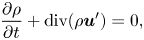 $$\begin{gather} \frac{\partial{\rho}}{\partial t} + \text{div} (\rho \boldsymbol{u}') = 0, \end{gather}$$
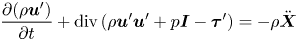 $$\begin{gather}\frac{\partial (\rho \boldsymbol{u}')}{\partial t} + \text{div} \, (\rho \boldsymbol{u}' \boldsymbol{u}' + p \boldsymbol{I} - \boldsymbol{\tau}') ={-} \rho \ddot{\boldsymbol{X}} \end{gather}$$
and
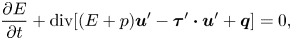 \begin{equation} \frac{\partial E}{\partial t} + \text{div} [(E + p) \boldsymbol{u}' - \boldsymbol{\tau}' \boldsymbol{\cdot} \boldsymbol{u}' + \boldsymbol{q} ] = 0 , \end{equation}
where  $\boldsymbol {X} = (0,h(t),0 )$ is the position of the non-inertial frame, and primed quantities represent variables measured with respect to the moving frame of reference. The total energy and the heat flux for a fluid obeying Fourier's law are
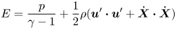 \begin{equation} E = \frac{p}{\gamma - 1} + \frac{1}{2} \rho ( \boldsymbol{u}' \boldsymbol{\cdot} \boldsymbol{u}' + \dot{\boldsymbol{X}} \boldsymbol{\cdot} \dot{\boldsymbol{X}} ) \end{equation}
and
 \begin{equation} \boldsymbol{q} ={-}\frac{\mu}{Re_a\,Pr } \, \text{grad} \, T , \end{equation}
respectively. Finally, the viscous stress tensor is given by
 \begin{equation} \boldsymbol{\tau}'= \frac{1}{Re_a} \big[ 2 \mu \boldsymbol{S}' - \tfrac{2}{3} \mu \, \text{div} \, \boldsymbol{u}' \boldsymbol{I} \big] , \end{equation}
where
 \begin{equation} \boldsymbol{S}' = \tfrac{1}{2} (\text{grad} \, \boldsymbol{u}' + (\text{grad} \, \boldsymbol{u}')^{\mathrm{T}}) \end{equation}
is the strain rate tensor, and  $Re_a = Re / M_\infty$ is the Reynolds number based on the speed of sound. Assuming the medium to be a calorically perfect gas, the set of equations is closed by the equation of state
 \begin{equation} p = \frac{\gamma - 1}{\gamma} \rho T . \end{equation}
It is worth mentioning that the code used in the present study has been validated previously for dynamic stall simulations by Ramos et al. (Reference Ramos, Wolf, Yeh and Taira2019).
2.2. Dynamic mode decomposition
Dynamic mode decomposition (DMD) (Schmid Reference Schmid2010; Tu et al. Reference Tu, Rowley, Luchtenburg, Brunton and Kutz2014) is a technique that isolates the most dynamically significant modes containing low-rank flow structures oscillating at a single frequency. The algorithm employed here builds upon the singular value decomposition (SVD) of the snapshot data and computes a finite-dimensional approximation of the infinite-dimensional Koopman operator (Tu et al. Reference Tu, Rowley, Luchtenburg, Brunton and Kutz2014).
In the algorithm, the dynamical system (which can be nonlinear) is reconstructed as a linear best-fit (least-squares) approximation  $\boldsymbol {X}' \approx \boldsymbol {A} \boldsymbol {X}$, with matrices $\boldsymbol {X}$ and $\boldsymbol {X}' \in \mathbb {C}^{m \times n-1}$, and we store the snapshots in columns as follows:
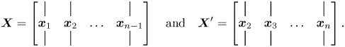 \begin{equation} \boldsymbol{X} = \left[ \begin{array}{@{}cccc@{}} | & | & & | \\ \boldsymbol{x}_{1} & \boldsymbol{x}_{2} & \ldots & \boldsymbol{x}_{n-1} \\ | & | & & | \end{array} \right] \quad \text{and} \quad \boldsymbol{X}' = \left[ \begin{array}{@{}cccc@{}} | & | & & | \\ \boldsymbol{x}_{2} & \boldsymbol{x}_{3} & \ldots & \boldsymbol{x}_{n} \\ | & | & & | \end{array} \right]. \end{equation}
Here,  $\boldsymbol {x}_{i}$, $i = 1, 2, 3,\ldots,n$, represent the snapshots, $m$ is the number of grid points, and $n$ is the total number of snapshots. Then the best-fit linear operator $\boldsymbol {A}$ and its eigendecomposition are evaluated to extract the DMD modes $\boldsymbol {\varPhi }$. The initial amplitudes of the individual modes, $b_k$, are computed such that the system can be approximated by
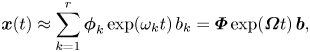 \begin{equation} \boldsymbol{x}(t) \approx \sum_{k=1}^{r} \boldsymbol{\phi}_k \exp(\omega_k t)\,b_k = \boldsymbol{\varPhi} \exp(\boldsymbol{\varOmega} t)\, \boldsymbol{b} , \end{equation}
where  $\omega _k = \ln (\lambda _k)/{\rm \Delta} t$ and $\boldsymbol {\varOmega }$ is a diagonal matrix whose entries are the $\omega _k$ values. The full algorithm is described in more details in Appendix A. This classical DMD approach has been used for analysing unsteady flow features in several applications, for example in jets (Semeraro, Bellani & Lundell Reference Semeraro, Bellani and Lundell2012), cavities (Seena & Sung Reference Seena and Sung2011), wakes (Muld, Efraimsson & Henningson Reference Muld, Efraimsson and Henningson2012) and detonation waves (Massa, Kumar & Ravindran Reference Massa, Kumar and Ravindran2012), and also in dynamic stall (Dunne et al. Reference Dunne, Schmid and McKeon2016; Mohan et al. Reference Mohan, Gaitonde and Visbal2016), as mentioned earlier. In this work, we also employ a recent variation of DMD labelled as multi-resolution DMD (mrDMD).
2.3. Multi-resolution dynamic mode decomposition
This algorithm variant consists of a recursive computation of DMD to remove low-frequency, or slowly varying, features from the collection of snapshots (Kutz et al. Reference Kutz, Fu and Brunton2016). Its primary advantage stems from its ability to separate long-, medium- and short-term trends in data. The resulting output, then, provides a means to better analyse transient or intermittent dynamics that the normal DMD fails to capture. Furthermore, the mrDMD is able to handle translational and rotational invariances of low-rank embeddings that are often undermined by other SVD-based methods.
In a wavelet-based manner, the time domain is divided into two segments recursively to create multiple resolution levels until a desired termination. Since only the lowest frequencies are removed from each bin, data can be sub-sampled to increase computational efficiency. Denoting by  $L$,
$L$,  $J$ and $m_l$ the number of decomposition levels, temporal bins per level, and modes extracted at each level $l$, respectively, the dynamical system is expressed as
 \begin{equation} \boldsymbol{x}(t) = \sum_{l=1}^{L} \sum_{j=1}^{J} \sum_{k=1}^{m_l} f^{l,j}(t)\,\boldsymbol{\phi}_k^{(l,j)} \exp(\omega_k^{(l,j)} t)\, b_k^{(l,j)} . \end{equation}
In the expansion above,  $f^{l,j}(t)$ is an indicator term that acts as a sifting function for each temporal bin and is defined as
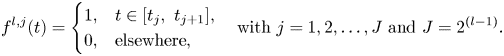 \begin{equation} f^{l,j}(t) = \begin{cases} 1, & t \in [t_j, \ t_{j+1}], \\ 0, & \text{elsewhere}, \end{cases} \quad \text{with } j = 1,2,\ldots,J \text{ and } J = 2^{(l-1)}. \end{equation}
Artificial high-frequency oscillations may be introduced by the hard cutoff of the time series in each sampling bin, but they are naturally filtered out by the lowest frequency selection during the recursion. For a detailed description of the mrDMD algorithm, the reader is referred to Kutz et al. (Reference Kutz, Fu and Brunton2016).
3. Results
Two different freestream Mach numbers are investigated in this work to assess compressibility effects on deep dynamic stall of a periodic plunging aerofoil. Simulations are performed for  $M_{\infty } = 0.1$ and $0.4$, the former also being studied by Visbal (Reference Visbal2011), Mohan et al. (Reference Mohan, Gaitonde and Visbal2016) and Ramos et al. (Reference Ramos, Wolf, Yeh and Taira2019). Mesh refinement and domain extension studies are discussed by the references previously cited, and in the present work we employ the grid resolution used by Ramos et al. (Reference Ramos, Wolf, Yeh and Taira2019), which has $480 \times 350 \times 96$ ( $\approx$ 16 million) points along a $z/c = 0.4$ span. An extensive literature (see, for instance, Visbal Reference Visbal2011; Visbal & Garmann Reference Visbal and Garmann2018; Benton & Visbal Reference Benton and Visbal2019, Reference Benton and Visbal2020) provides compelling evidence that this spanwise extension is sufficient to capture accurately the aerodynamic loadings and the relevant dynamics associated with the dynamic stall onset. The studied configuration comprises an SD7003 aerofoil at $\alpha _0 = 8^{\circ }$ static angle of attack. The aerofoil trailing edge is rounded with an arc of radius $r/c = 0.0008$ to facilitate the use of an O-mesh topology and to keep metric terms smooth.
It is worth mentioning that in this work, we employ the numerical method and grid used by Ramos et al. (Reference Ramos, Wolf, Yeh and Taira2019) for the  $M_{\infty } = 0.1$ flow, whose results compare well with those from Visbal (Reference Visbal2011), in terms of both local flow structures and integrated loads. However, in order to validate the results for $M_{\infty } = 0.4$, a refined grid of size $576 \times 444 \times 120$ ( $\approx$ 31 million points) was designed to have 25–40 % improvement in resolution on the suction side, depending on the direction, after a localized distribution of points. Computations showed an excellent agreement between the two grids, hence results will be shown only for the smaller grid.
The aerofoil vertical displacement  $h(t)$ is specified as a function of non-dimensional time $t$, reduced frequency $k$, and maximum plunge amplitude $h_0$, as
 \begin{equation} h(t) = h_0 \sin(2kt).\end{equation}
Here, the parameters are set as  $k= 0.25$ and $h_0 = 0.5$ to reproduce the deep stall flow configuration studied by Visbal (Reference Visbal2011) and Ramos et al. (Reference Ramos, Wolf, Yeh and Taira2019). Although the numerical formulation uses a non-dimensionalization of flow velocities and time scale by speed of sound, the parameters in (3.1) are based on the freestream velocity, similar to the previous references. The maximum plunging amplitude is normalized by the chord length and the aerofoil undergoes a variation in effective angle of attack in the range $-6^{\circ } \leq \alpha _{eff} \leq 22^{\circ }$.
For the present plunging aerofoil at  $M_{\infty } = 0.1$, Ramos et al. (Reference Ramos, Wolf, Yeh and Taira2019) show that discarding the first cycle is sufficient to remove transient features from the numerical procedure, which assumes an initial uniform flow in the entire domain. We performed the computation of another cycle for $M_{\infty } = 0.4$ and observed similar changes in the aerodynamic coefficients compared to those shown by Ramos et al. (Reference Ramos, Wolf, Yeh and Taira2019). Hence results are shown for the second cycle, and although cycle-to-cycle variations indeed occur, we emphasize that the effort here is to focus on the onset of dynamic stall, where one cycle should be sufficient to capture the main trends associated with the formation of the DSV. Phase-averaged results of this case can be found in Visbal (Reference Visbal2011) and Ramos et al. (Reference Ramos, Wolf, Yeh and Taira2019), and the effects of cycle-to-cycle variations are discussed by the latter authors. It is also important to note that, differently from the previous references, here we define the reference position for the phase angle $\phi =0^{\circ }$ at $h(t) = 0$ and not at the topmost position $h(t) = h_0 = 0.5$. Therefore, at $\phi =0^{\circ }$, the aerofoil is moving upwards with maximum vertical velocity. The aerofoil reaches the top-most position at $\phi =90^{\circ }$ with zero vertical velocity, and then starts the descending motion. At $\phi =180^{\circ }$ it has the maximum downward velocity, and at $\phi =270^{\circ }$ it reaches the bottom-most position. Then it moves upwards and repeats the cycle.
3.1. General flow features
Figure 1 shows the lift ( $C_l$), drag ( $C_d$) and pitching moment ( $C_m$) coefficients as functions of the effective angle of attack for freestream Mach numbers $M_\infty = 0.1$ and $0.4$. The dashed blue lines indicate the phase-averaged coefficients obtained by Visbal (Reference Visbal2011) after six cycles, for $M_\infty = 0.1$. From this figure, good agreement is observed between the present results and those from Visbal, despite the differences in the numerical methods, computational grids and phase-averaging effects. At this point, it is important to reiterate that our results display the aerodynamic loadings for a single cycle, and that they lie within the cycle-to-cycle variations shown in Visbal's work. The dashed red lines, in turn, stand for the results obtained by one cycle of the $M_\infty = 0.4$ flow with the finer grid. Differences observed are due to the sensitivity of the flow to the initial conditions, as would occur due to cycle-to-cycle variations. The phase angle $\phi$ is also shown in the plots for particular instants of the motion, and the circle and cross symbols on the $C_l$ and $C_d$ plots mark the dynamic stall onset time based on different criteria (further details are provided in § 3.3). It is observed that compressibility acts on the sense to attenuate the aerodynamic loads in the hysteresis loop while maintaining their maximum and minimum values, a trend that was also observed by Sangwan et al. (Reference Sangwan, Sengupta and Suchandra2017) for a two-dimensional simulation of a pitching aerofoil. Here, we observe that the largest changes in $C_l$ and $C_d$ occur when the effective angle of attack is reduced from $\alpha _{eff} \approx 18^{\circ }$ to $10^{\circ }$, which corresponds to the time interval when the aerofoil is ceasing its downstroke motion. At $\alpha _{eff} = 8^{\circ }$, the aerofoil is at the bottom-most position for the downstroke.
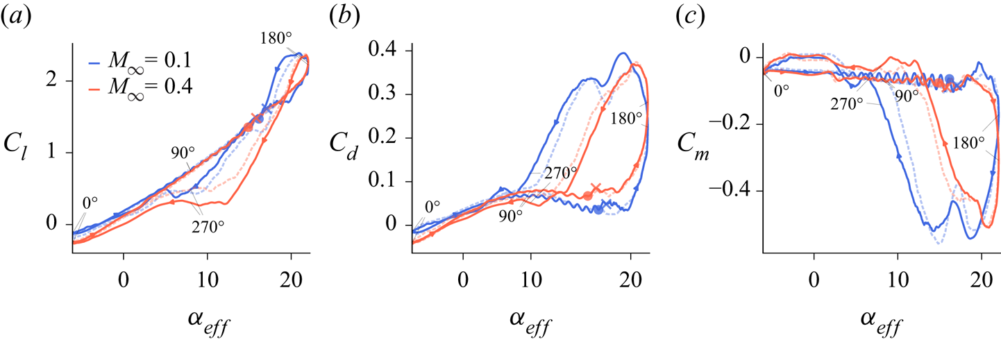
Figure 1. (a) Lift, (b) drag and (c) pitching moment coefficients, as functions of the effective angle of attack for  $M_\infty = 0.1$ and $0.4$. Dashed blue lines are phase-averaged results from Visbal (Reference Visbal2011), and dashed red lines are results for $M_\infty = 0.4$ with a finer grid. Circle and cross symbols represent onset time based on LESP and ${\rm \Delta} z$ criteria, respectively (see § 3.3).
These results, especially the accentuated decay of the coefficients during the post-stall period with the increasing Mach number, can be understood better from figures 2 and 3. The former exhibits the spanwise-averaged pressure coefficient ( $C_p$) contours at different flow instants for the two Mach numbers investigated (figures 2a,b) and its distribution over the aerofoil suction side (figure 2c). The formation of the DSV is also shown in grey shading using a flow entropy measure defined as $(p/p_0)/(\rho /\rho _0)^{\gamma } - 1$, where $p_0 = 1/\gamma$ and $\rho _0 = 1$ are reference values for pressure and density, respectively. This entropy measure gives a better visual representation of the separated flow since it indicates the regions where entropy is changing due to viscous effects. Figure 3 presents the full history of pressure ( $C_p$) and skin friction ( $C_f$) coefficients along the suction side of the aerofoil.
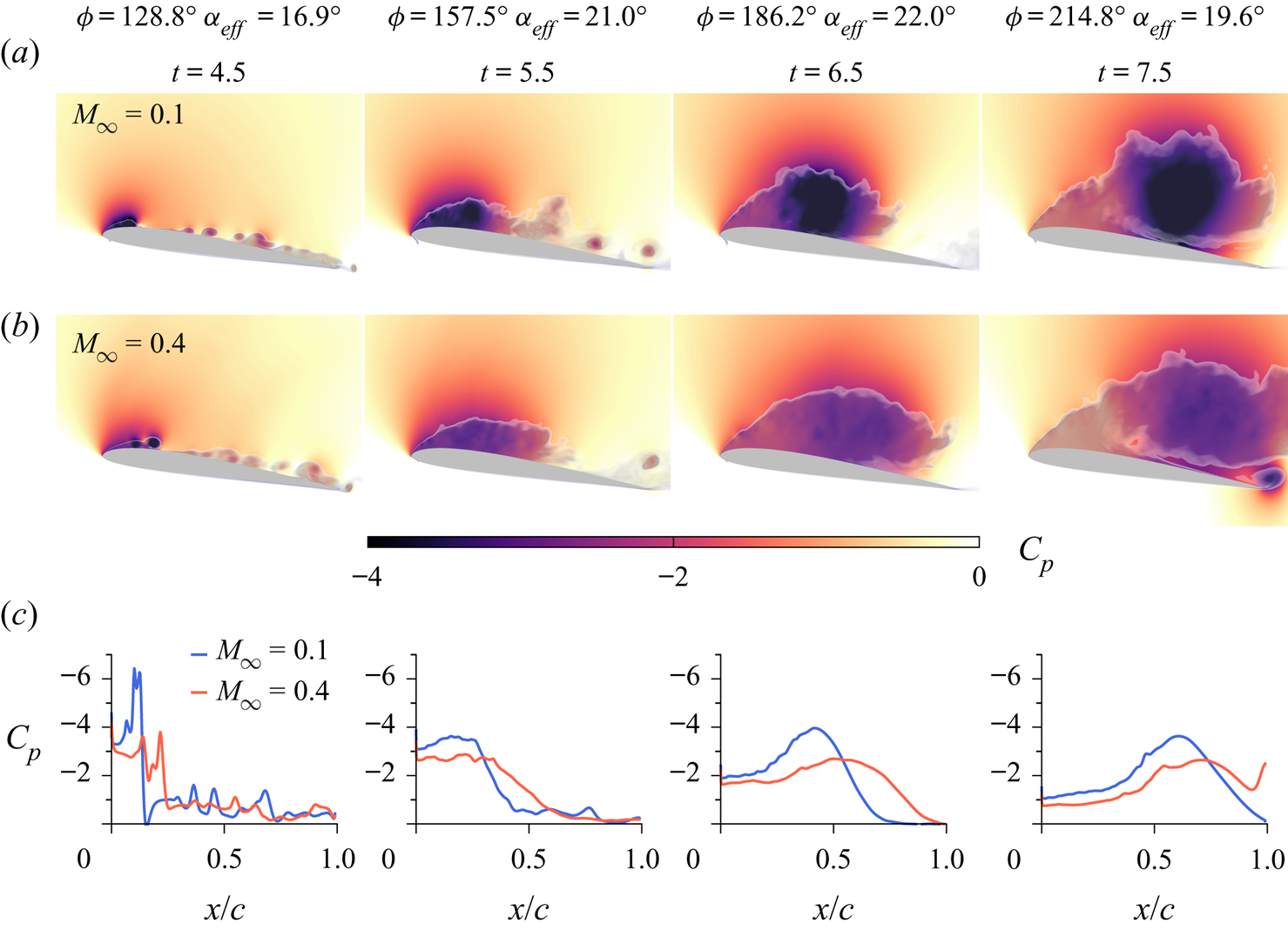
Figure 2. Spanwise-averaged pressure coefficients at different flow instants for (a)  $M_{\infty } = 0.1$, and (b) $M_{\infty } = 0.4$; and (c) $C_p$ over the aerofoil suction side. The evolution of the DSV can be seen in a movie (supplementary movies are available at https://doi.org/10.1017/jfm.2022.165).
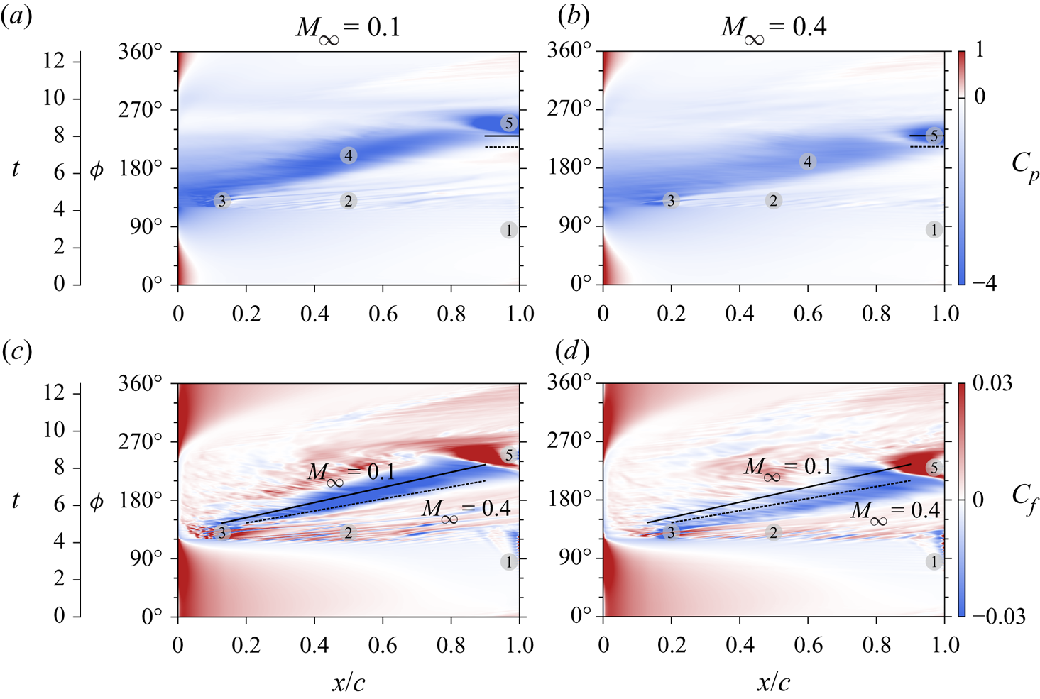
Figure 3. Comparison of (a,b) pressure and (c,d) skin friction coefficients for (a,c)  $M_{\infty } = 0.1$ and (b,d) $M_{\infty } = 0.4$. Auxiliary lines and markers are included to facilitate the comparison between the two flows and to represent specific events as described in the text.
From figure 2, two observations can be drawn immediately. The first is that the suction peak is reduced near the leading edge for the higher Mach number flow, as demonstrated in figure 2(c) for  $t=4.5$. This condition is accompanied by a weaker, more diffuse, pressure core of the DSV. The second observation concerns the gestation period and residence time for which the DSV remains over the aerofoil. Heuristic reasoning to explain the weakening of the DSV strength with compressibility is provided by Chandrasekhara & Carr (Reference Chandrasekhara and Carr1990). They argue that for higher Mach numbers, the pressure gradient is reduced near the leading edge due to the smaller curvature of the streamlines from the earlier flow separation. At this condition, the net vorticity introduced is lower, which leads to a weaker vortex formation. With respect to the second observation, figure 2 shows that the DSV residence time is smaller for $M_{\infty } = 0.4$, and that it is more spread at $t=6.5$, spanning a larger region over the aerofoil suction side. On the other hand, the DSV is relatively concentrated at the mid-chord location for the lower Mach number case. At $t=7.5$, the DSV is already leaving the aerofoil surface for the higher Mach number flow, followed by a trailing edge vortex.
The same conclusions can be drawn from the map of  $C_p$ over the aerofoil suction side, depicted in figures 3(a,b). In this $x/c$– $t$ diagram, the dark blue contours represent the signature of the DSV over the aerofoil suction side followed by the formation of the trailing edge vortex. We observe that the $C_p$ contours are lighter for $M_{\infty } = 0.4$ (see marker 4 in the figures), indicating the presence of a weaker pressure core. Moreover, with closer inspection, it is possible to measure a delay of $17^{\circ }$ in the phase angle between the formation of the trailing edge vortex for the two Mach number flows, as indicated by the horizontal black lines on marker 5. The solid and dashed horizontal lines show the initial formation of the trailing edge vortex for the $M_{\infty } = 0.1$ and $0.4$ cases, respectively. While the trailing edge vortex starts to form at $\phi = 213^{\circ }$ for $M_{\infty } = 0.4$, its appearance occurs at $\phi = 230^{\circ }$ for $M_{\infty } = 0.1$.
The  $C_f$ plots in figures 3(c,d) present further information about the flow history over the suction side of the aerofoil. At about $90^{\circ }$ phase angle, an oscillatory pattern appears close to the aerofoil trailing edge as shown by marker 1. These oscillations arise due to initial shedding of von Kármán vortices from the aerofoil trailing edge, which exhibit a higher frequency at the lower Mach number flow. This vortex shedding can be visualized better in a movie (see supplementary movies). In the following moments, high-frequency $C_f$ variations can be observed spanning almost the entire chord (denoted by marker 2) in the range $120^{\circ } <\phi < 130^{\circ }$ for both flow conditions, but they are more pronounced for the $M_{\infty } = 0.1$ case. These fluctuations are due to Kelvin–Helmholtz instabilities forming during the downstroke motion. Figure 4 shows this primary instability stage of the flow at different instants using entropy contours. As is evident, initially the instabilities arise closer to the trailing edge, but they develop rapidly along the entire suction side. They appear to form at an earlier time for the lower Mach number and exhibit a more organized and denser behaviour where flow structures display a higher wavenumber.
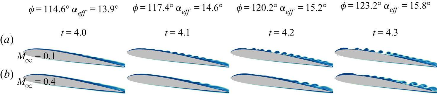
Figure 4. Entropy contours showing the development of Kelvin–Helmholtz instabilities (here called the primary instability stage) along the aerofoil suction side for (a)  $M_{\infty } = 0.1$, and (b) $M_{\infty } = 0.4$.
For both cases investigated, the formation of the dynamic stall vortex appears just after the Kelvin–Helmholtz instabilities approach the leading edge, at phase angle  $\phi \approx 135^{\circ }$, shown by marker 3 in figure 3. In the same figure, the travelling signature of the DSV is shown by the negative $C_f$ values shown in blue contours along the aerofoil chord for intermediate phase angles $\phi$. Auxiliary black lines are included to facilitate the comparison of the mean velocity at which the DSV is being transported for each compressible regime. The lines represent an approximate path of the DSV when moving, considering the centre of the blue region. The solid line corresponds to the DSV signature of the $M_{\infty } = 0.1$ flow, while the dashed line refers to the $M_{\infty } = 0.4$ case. They are repeated in both subplots to facilitate the comparison of their slopes, and show that the DSV is being advected faster in the higher Mach number flow. The weaker signature of friction coefficient for $M_{\infty } = 0.4$ is also noticeable compared to that for $M_{\infty } = 0.1$.
The skin friction maps in figure 3 also display the presence of a flow reversal at earlier times that progressively advances over the aerofoil suction side from the trailing edge towards the leading edge as  $\phi$ increases. This region appears for $\phi \leq 120^{\circ }$ in light blue contours, below markers 1, 2 and 3. The time (here also visualized as a function of the plunge cycle angle $\phi$) in which the flow reversal initiates does not appear to change under the distinct compressible regimes investigated. The main differences in $C_f$ between the two flows start after the beginning of the primary instabilities (marker 2), which are more sparse for the higher Mach number flow. As mentioned before, the transport of the DSV over the suction side is faster for $M_{\infty } = 0.4$, and its signature is more diffuse. Moreover, the point where the development of the DSV occurs changes from approximately $x/c = 0.1$ for $M_{\infty } = 0.1$ to $x/c = 0.2$ for $M_{\infty } = 0.4$ (see different positions of marker 3). This behaviour can be understood better through an inspection of the boundary layer forming over the aerofoil suction side.
3.2. Onset of dynamic stall
Figure 5 shows the spanwise-averaged  $z$-vorticity contours in a short time window that marks the moment of formation of the DSV. As can be seen from the figure, ${\rm \Delta} t = 0.3$ based on the freestream velocity, which corresponds to nearly 2.4 % of the plunging cycle period. Unlike for steady separation, in dynamic stall the outer flow continues to follow the aerofoil contour despite the presence of flow reversal. As a consequence, a local shear layer forms between the displaced leading edge boundary layer and the reversed fluid layer that is, at a later stage, subjected to inflectional instabilities. This leads to the generation and growth of coherent structures that can be visualized in figure 5 and in a movie (see supplementary movies). In the figure, auxiliary lines are plotted to indicate regions where $u$- and $v$-velocity components change direction, from which we identify the presence of flow reversal and the shear layer over the leading edge.
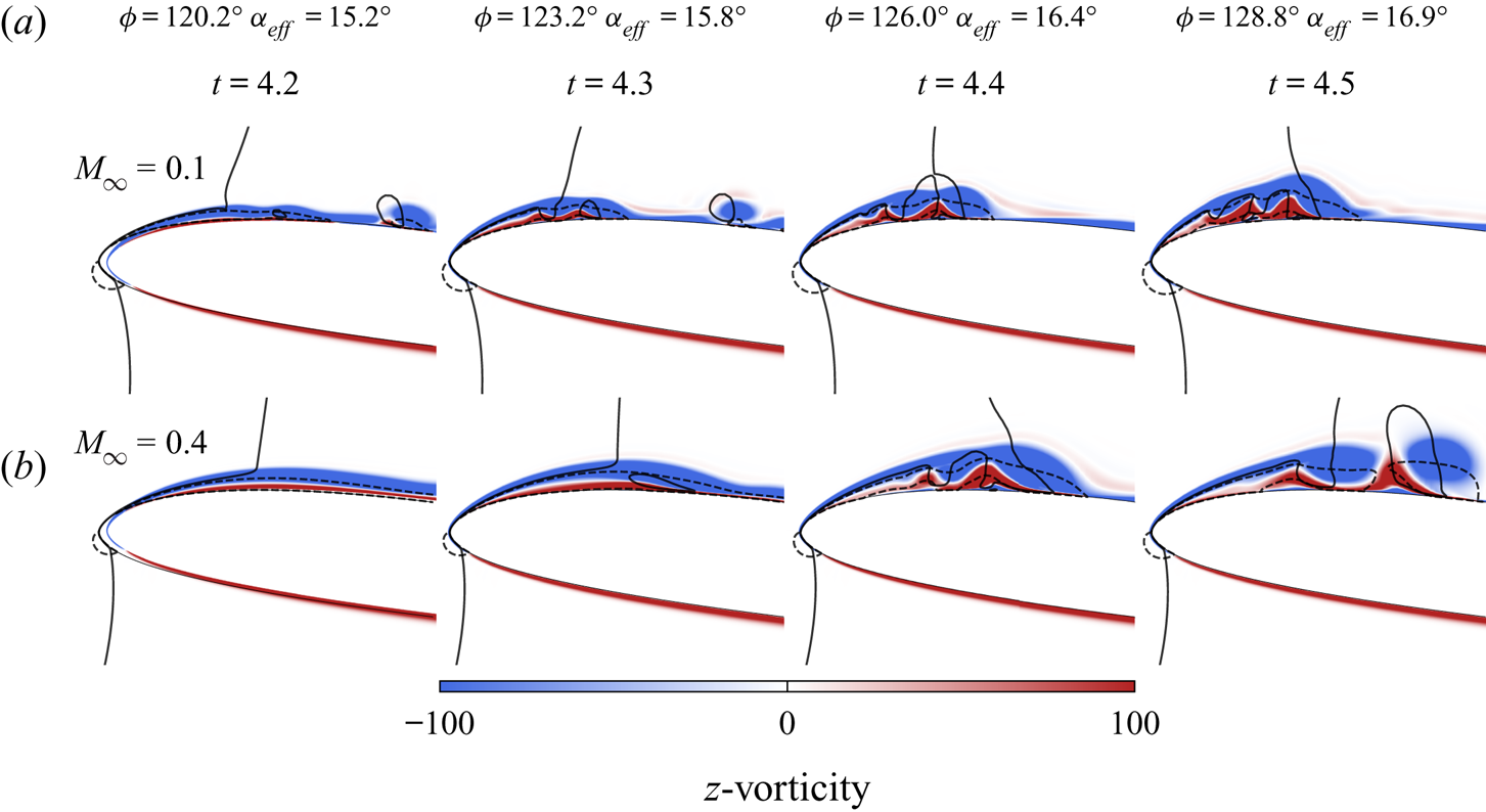
Figure 5. Spanwise-averaged  $z$-vorticity field near the leading edge ( $x/c \le 0.25$) revealing the sudden boundary layer separation for (a) $M_{\infty } = 0.1$, and (b) $M_{\infty } = 0.4$. Dashed and solid lines represent the boundaries for which $u=0$ and $v=0$, respectively, indicating flow regions where velocity components change direction.
In previous work by van Dommelen & Shen (Reference van Dommelen and Shen1980), it is speculated that the onset of the unsteady separation phenomenon is an inviscid process, independent of the Reynolds number. This characteristic is attributed to the fact that the initial flow reversal near the surface, which is triggered by a strong adverse pressure gradient, is later governed by inertial effects on the zero-vorticity line. Along this line, formed as the fluid approaches the separation region, the convective terms dominate the viscous effects, justifying the inviscid assumption. Under the influence of the increasing adverse pressure gradient, the local reversed flow begins to accelerate rapidly upstream near the leading edge region, generating an intense shear. Because of the presence of the solid surface, fluid is propelled away from the wall. Meanwhile, the vorticity conservation yields an outward distortion of the zero-vorticity line, destabilizing the local vorticity distribution and resulting in the formation of a large vortical structure. The development of this vortex and its induced secondary separation leads to its ejection from the surface.
The process described above is visualized in figure 6 and in a movie (see supplementary movies), where the local Mach number is plotted along with the zero-vorticity lines during the dynamic stall onset. In this figure, a straight line measuring  $0.06 c$ in length is plotted normal to the aerofoil surface, from which tangential and normal velocity components are computed to describe the evolution of the local velocity field. The placement of these lines is chosen in order to highlight similar behaviour of the velocity field at $t=4.4$, but since separation occurs at different chord positions depending on the freestream Mach number, they are placed at different distances from the aerofoil leading edge for each flow. The values $x/c = 0.11$ and $0.15$ are chosen for $M_{\infty }=0.1$ and $M_{\infty }=0.4$, respectively. We stress that these values are meant not to indicate the precise location of the separation, but only to help to illustrate the van Dommelen and Shen model. With that clarification, figure 7 shows the profiles of tangential ( $u_t$) and normal ( $u_n$) velocity components in blue and red, respectively. The corresponding vectors are also displayed in the figure. The tail of each vector is placed at the respective normal distance where its velocity components are shown.
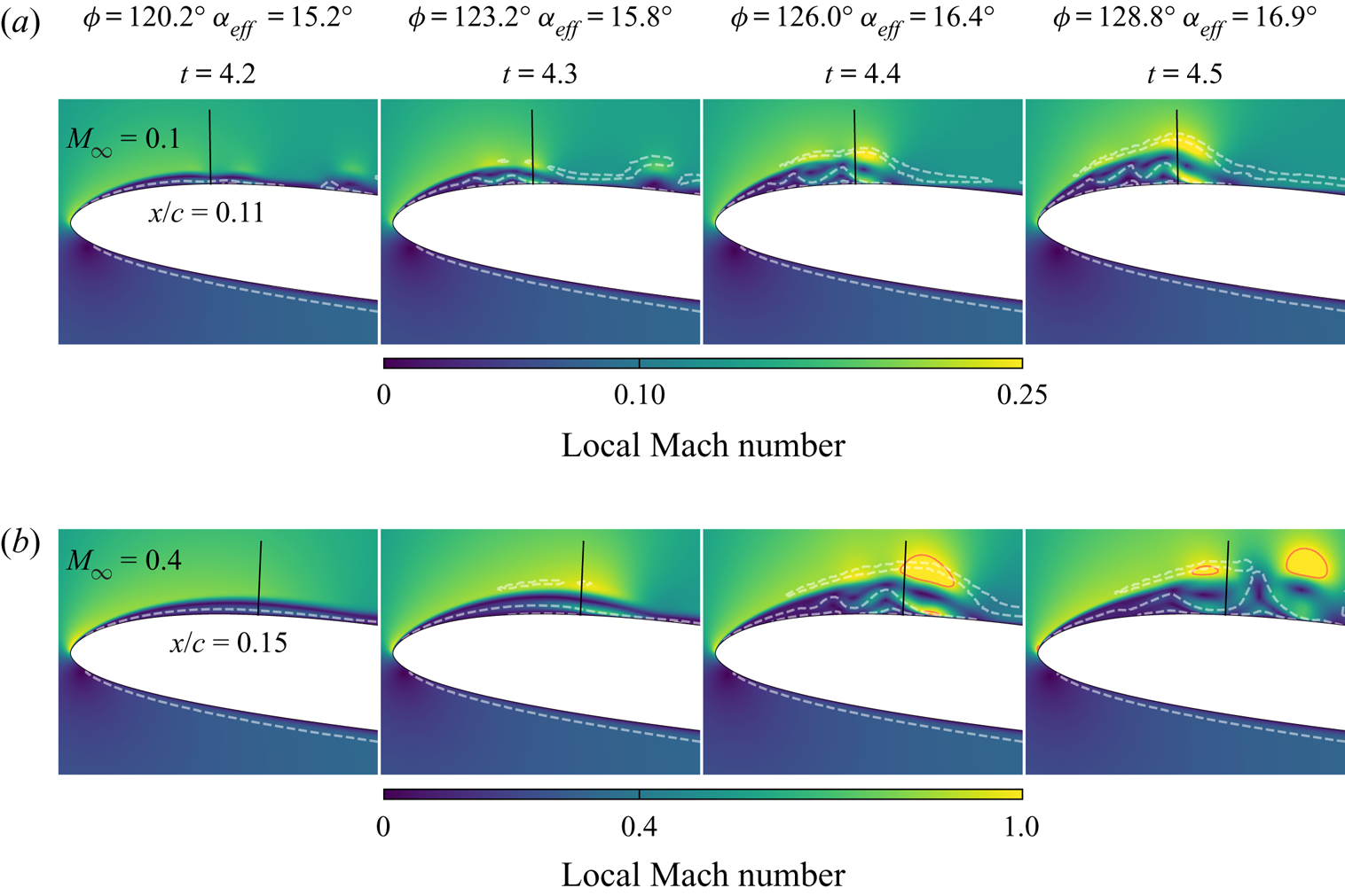
Figure 6. Local Mach number contours near the leading edge ( $x/c \le 0.25$) for (a) $M_{\infty } = 0.1$, and (b) $M_{\infty } = 0.4$. White dashed lines represent the zero-vorticity lines, and solid red lines represent regions of sonic flow.
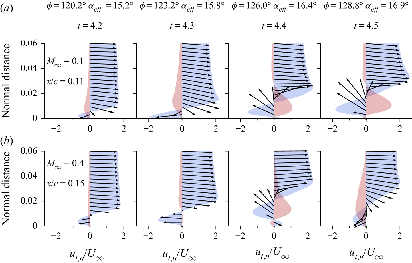
Figure 7. Tangential ( $u_t$, blue) and normal ( $u_n$, red) velocity profiles for (a) $M_{\infty } = 0.1$, and (b) $M_{\infty } = 0.4$.
In figure 6, the flow continues to accelerate up to a point further downstream of the leading edge where it encounters the reversed flow accelerating along the inner layer in the opposite direction. This acceleration is also evident in the increment of the tangential velocity between the first and second columns in figure 7. In this region, a mutual interaction is apparent between the outer flow and the flow inside the zero-vorticity line to form a low-pressure core (not shown). At  $M_{\infty }=0.4$, the strong acceleration of the reversed flow is sufficient to achieve sonic speeds along the zero-vorticity lines (red lines in figure 6 represent regions of $M = 1$). The flow, however, is decelerated almost isentropically, and no shock waves are observed despite the sonic flow regions. The strong shear accompanied by the low pressure on the aft portion of the separation region results in the flow reversal being ejected away from the surface, as shown by the velocity vectors in the third and fourth columns of figure 7. The interaction of the ejected flow with the outer flow creates a vortical structure that intensifies the instabilities in the region. The dynamics observed in figures 5 and 6 appear to agree well with the overall concept of the van Dommelen and Shen model, which provides the description of the flow up to the early stages of separation.
As observed from the previous figures, the onset of the DSV appears further downstream from the leading edge with an increase in Mach number, as was also reported by Chandrasekhara & Carr (Reference Chandrasekhara and Carr1990) and Benton & Visbal (Reference Benton and Visbal2020) for pitching aerofoils. In their work, compressibility caused the leading edge separation to occur at an earlier time and, consequently, at a lower effective angle of attack. Therefore, the separation for higher Mach number flows would experience a less pronounced curvature of the streamlines and a weaker pressure gradient. However, this earlier separation is not observed in our simulations at  $Re = 6 \times 10^{4}$, suggesting that the pressure gradient reduction may not be a direct consequence of the lower effective angle of attack. It is important to mention that the observations from the previous authors are for higher Reynolds numbers than that considered in the present work.
For the present periodic plunging motion, the leading edge separation seems to be related to the primary instabilities developing at the trailing edge region and, later, spanning the entire aerofoil suction side as shown in figure 4. These instabilities approach the leading edge and interact with the secondary instability presented in figures 5 and 6. Notice that the term ‘secondary instability’ does not refer to the jargon commonly used in classical stability analysis. This term is used here only to differentiate the leading edge instability from the Kelvin–Helmholtz one. In particular, we notice from figure 4 that the primary instabilities reach further upstream for the  $M_{\infty }=0.1$ case. On the other hand, for $M_{\infty }=0.4$, a wider favourable pressure gradient region along the leading edge causes the formation of secondary instabilities to be shifted downstream over the aerofoil suction side and slightly delayed in time (see the first two columns of figure 5). This is illustrated in figure 8, which shows the instantaneous covariant derivative of pressure along the aerofoil. The variable $\xi = \xi (x,y)$ is the curvilinear coordinate of the O-mesh topology, which goes along the aerofoil profile, and $\mathrm {d}\xi / | \mathrm {d}\xi |$ is introduced to remove the influence of the mesh orientation of the covariant derivative. The basis of the curvilinear system is also normalized to yield a scale in physical units. As discussed in the literature (Li et al. Reference Li, Komperda, Ghiasi, Peyvan and Mashayek2019), compressibility has a stabilizing effect that delays the laminar to turbulence transition in free shear flows. Here, the mechanism appears to be similar, although the plunging motion together with the surface presence lead to a more complex flow.
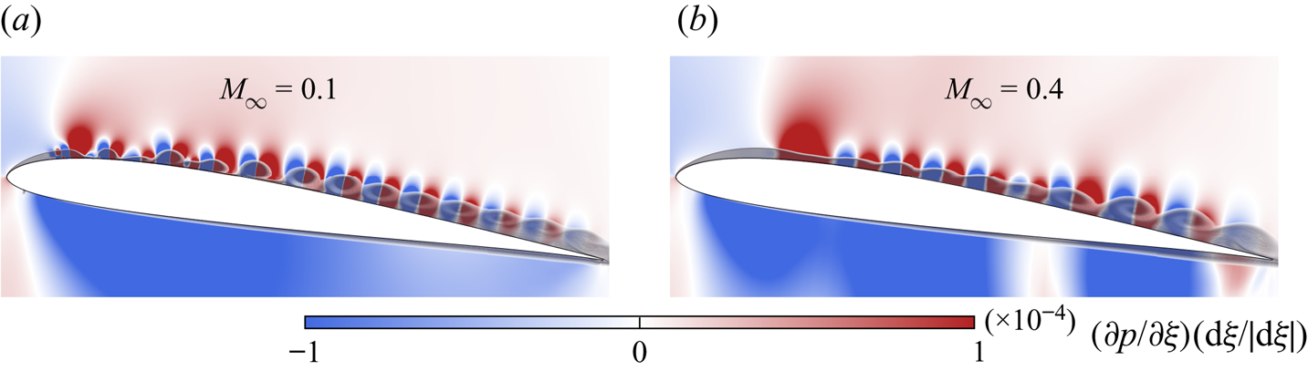
Figure 8. Pressure gradient contours (blue and red) in the streamwise  $\xi$ direction and contours of entropy (transparent shading) for (a) $M_{\infty } = 0.1$,and (b) $M_{\infty } = 0.4$, at $t=4.25$.
Given the importance of the pressure gradient on the dynamic stall onset, we display the pressure gradient history along the  $\xi$ direction over the aerofoil suction side in figure 9. The saturation level is kept high to call attention to the features marked in the figure. As can be confirmed from the movie (see supplementary movies), von Kármán vortices are shed from the aerofoil trailing edge before the primary instability stage. These vortices induce flow fluctuations that are scattered by the trailing edge generating acoustic waves that propagate upstream. These waves are perceived as the white ribbons in marker 3. The traces of the acoustic waves start at $\phi \approx 60^{\circ }$ and can be observed up to $\phi \approx 120^{\circ }$. The black arrows are tangent to their traces, and it is possible to conclude that for the $M_{\infty } = 0.4$ flow, the acoustic waves propagate upstream at a lower speed than for $M_{\infty } = 0.1$ due to the Doppler effect. Moreover, the larger thicknesses of the ribbons reflect the fact that the frequency at which the acoustic waves are generated is lower for $M_{\infty } = 0.4$. The arrows also show the path taken by a particular wave that coincides with the inception of the Kelvin–Helmholtz instabilities for each flow (the latter being represented by marker 2). The black circles in both subplots are positioned in the same spatio-temporal coordinates, emphasizing that the mechanism that creates the primary instability originates from the trailing edge at the same time for the two compressible regimes. However, since the upstream propagation speed of the acoustic wave is lower for the higher Mach number, the perturbation takes longer to reach $x/c=0.65$, where the Kelvin–Helmholtz instability starts. This chord location appears to be the same for both flows and is represented by the vertical dashed line in each subplot. In the region of marker 2, we observe the Kelvin–Helmholtz instabilities that, analogously to what happens with the acoustic waves, display a lower frequency for $M_{\infty } = 0.4$.
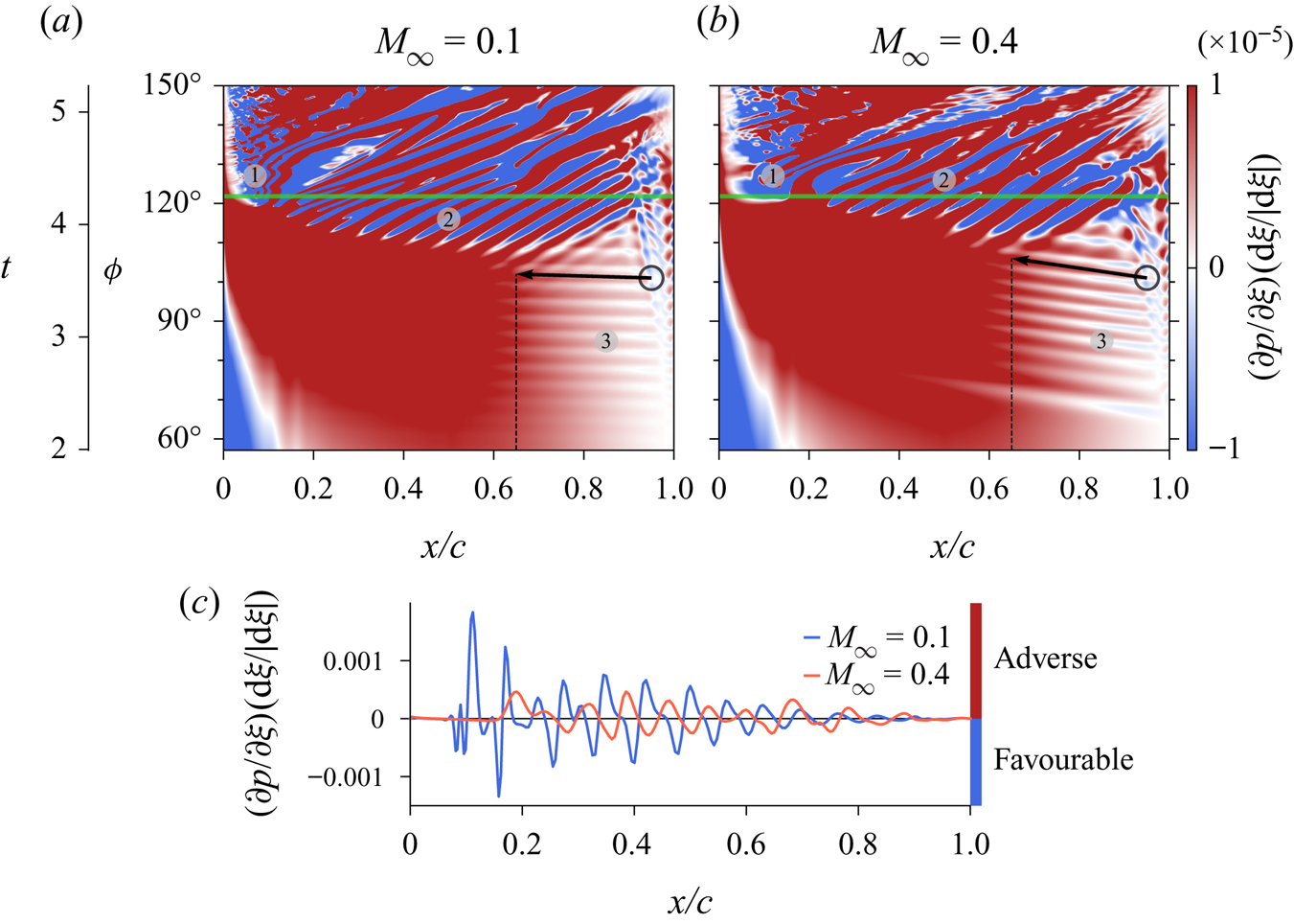
Figure 9. History of pressure gradient in the  $\xi$ direction over the aerofoil suction side for (a) $M_{\infty } = 0.1$, and (b) $M_{\infty } = 0.4$. Panel (c) shows the pressure gradients computed along the horizontal green line, which corresponds to $t=4.25$.
Shih, Lourenco & Krothapalli (Reference Shih, Lourenco and Krothapalli1995) pointed out that although a flow reversal extends from the trailing edge over the aerofoil suction side, there was insufficient time for this flow to reach the leading edge region. Therefore, they postulated that the flow reversal near the leading edge and the eventual initiation of the unsteady separation were essentially local phenomena. The trailing edge, in turn, was considered responsible for influencing the separation indirectly, through the increase of global circulation around the aerofoil by shedding counter-rotating vorticity into the wake. In our compressible simulations, the importance of the trailing edge lies in what appears to be the acoustic triggering of Kelvin–Helmholtz instabilities, but it is unclear whether the trailing edge is of secondary importance to the onset of the DSV. The Kelvin–Helmholtz instabilities occur due to shear, but our results suggest that the trailing edge acoustics might act as an initial disturbance that triggers the formation of such instabilities. Moreover, at marker 1 in figure 9, we see that the onset of the DSV occurs at nearly the same time for the two regimes, as do the acoustic waves that possibly trigger the primary instability. Since these latter propagate at different speeds, this means that the acoustic disturbance does not influence directly the dynamic stall onset. On the other hand, separation occurs only when the primary instability reaches the leading edge region, and the trailing edge seems to be important in the generation of this primary instability. Other studies (Benton & Visbal Reference Benton and Visbal2020) have shown that the turbulent separation from the trailing edge can play an important role in the dynamic stall onset depending on the flow configuration. However, such trailing edge separation is not present in our results.
In order to better assess the differences in pressure gradient between the two flows, we plot the values of the  $\xi$ pressure gradient component over the horizontal green line displayed in figure 9, which corresponds to $t=4.25$. The time instant is the same as that shown in figure 8, which displayed a wider region of favourable pressure gradient along the leading edge for $M_{\infty } = 0.4$. This more extensive region of favourable pressure gradient delays the formation of secondary instabilities in the higher Mach number case. From the figure, we can see that the adverse pressure gradient region (positive values) is shifted downstream from the leading edge at higher Mach number. We also notice that the magnitudes of the pressure gradient fluctuations are higher for the $M_{\infty } = 0.1$ case. In addition, high frequency oscillations and a strong peak appear close to the leading edge for $M_{\infty } = 0.1$. These are related to the beginning of the destabilization of the local vorticity distribution described by the van Dommelen and Shen model. Finally, this plot provides another interesting observation about the wavelengths of the Kelvin–Helmholtz instabilities: for the higher Mach number case, longer wavelengths are observed near the trailing edge region (say $x/c > 0.6$), while shorter ones can be seen around the mid-chord. For the lower Mach number flow, on the other hand, the wavelengths appear to be more uniform. Since our results are presented in terms of spanwise-averaged quantities, this fact possibly indicates a higher three-dimensionality of the flow structures close to the trailing edge for $M_{\infty } = 0.4$.
In a recent work by Benton & Visbal (Reference Benton and Visbal2020), simulations of a static NACA 0012 at  $8^{\circ }$ angle of attack and $Re = 10^{6}$ showed the presence of a wider spectrum of three-dimensional (oblique) modes in the transition process at the leading edge as compressibility was increased. Based on their observations, we investigate the presence of three-dimensional disturbances in the flow for the current plunging aerofoil. Results are shown in figure 10, where iso-surfaces of $q$-criterion $Q=1/2( |\varOmega |^{2} - |S |^{2} )$, coloured by $x$-momentum, are plotted over the aerofoil suction side. The figure is presented for $t=4.4$, which corresponds to a moment before the ejection of the first leading edge vortex (see third column of figure 6). Results show that the higher Mach number flow is more three-dimensional along the entire aerofoil suction side. Given the quicker breakup of spanwise coherence of Kelvin–Helmholtz instabilities for $M_{\infty } = 0.4$, it could be that non-normality plays an important role in this case. Even the leading edge vortices related to the secondary instability mechanism display spanwise modes at this higher Mach number. On the other hand, the rolls of the $M_{\infty } = 0.1$ flow are mostly two-dimensional, except close to the trailing edge where transition sets in.
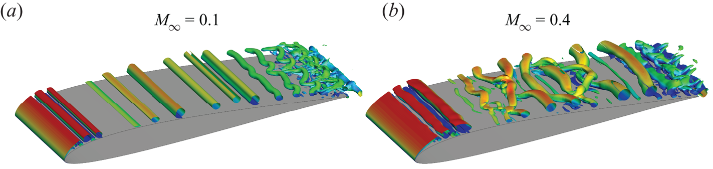
Figure 10. Iso-surfaces of  $q$-criterion coloured by $x$-momentum for (a) $M_{\infty } = 0.1$, and (b) $M_{\infty } = 0.4$, computed at $t=4.4$.
3.3. Analysis of empirical criteria for dynamic stall onset
As discussed by Ramesh et al. (Reference Ramesh, Gopalarathnam, Granlund, Ol and Edwards2014), the LESP  $A_0$ can be used to indicate the onset of the DSV, which occurs when the maximum value of this parameter is achieved. According to Deparday & Mulleners (Reference Deparday and Mulleners2019), the LESP can be computed directly from numerical or experimental data as
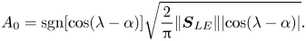 \begin{equation} A_{0} = \text{sgn}[\cos(\lambda - \alpha)] \sqrt{ \frac{2}{{\rm \pi} } |\boldsymbol{S}_{LE} | |{\cos(\lambda - \alpha)}|} . \end{equation}
In (3.2),  $\alpha$ is the effective angle of attack, and $\lambda$ is the angle formed between the incoming flow and the leading edge suction vector $\boldsymbol {S}_{LE}$. This vector is determined by integrating the pressure signals along the first 10 % of the aerofoil chord. Hence $\boldsymbol {S}_{LE}$ gives the net force from the surface pressure integration. Here, the sign function is included to yield a continuous result when $\cos (\lambda - \alpha )$ goes from positive to negative, and vice versa. A schematic representation of the terms used to evaluate $A_{0}$ according to Deparday & Mulleners (Reference Deparday and Mulleners2019) is presented in figure 11(a). In this figure, the 10 % frontal portion of the aerofoil chord is coloured blue, and the chord line is shown by a dashed line.
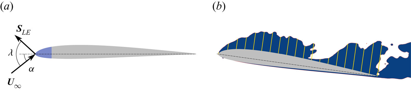
Figure 11. Schematic of the relevant parameters used in the calculation of (a) the LESP, and (b) an entropy measure showing the evaluation of the chord-normal shear layer height.
The temporal evolution of the LESP for the periodic aerofoil motion is shown in figure 12(a) for the two Mach numbers investigated. Relevant values of the phase angle  $\phi$ are marked in the figure, and the green and purple dots are the LESP thresholds, plotted along with their respective coordinates $(t, A_{0})$. The green dots represent the first local maxima found in $A_0$, while the purple dots show the global maximum. According to the previous references, the global maximum should indicate the instant of the DSV onset. However, we find here that the first local maximum provides a better estimate for the onset. Deparday & Mulleners (Reference Deparday and Mulleners2019) show that after the onset of the DSV, the LESP is susceptible to fluctuations from the separated flow. Moreover, the secondary instabilities develop downstream 10 % of the chord in the present flows. These characteristics could impact on the calculation of the LESP, since they may lead to new maximum values. Hence the green dots will be used to provide the time instant of dynamic stall onset.
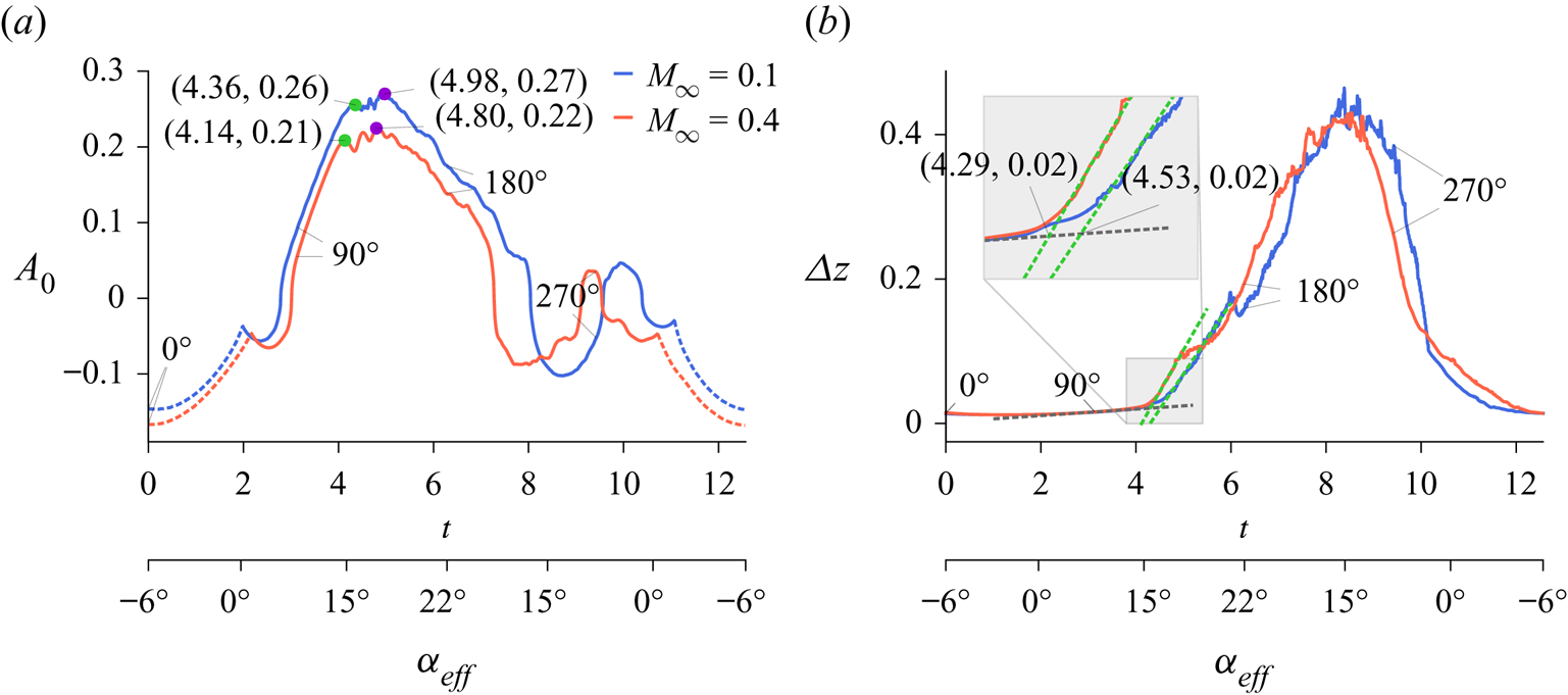
Figure 12. (a) LESP, and (b) chord normal shear layer height, for the aerofoil in periodic motion at  $M_{\infty } = 0.1$ and $0.4$.
Comparing the blue and red lines from figure 12, which correspond to the values of  $A_{0}$ for Mach numbers $M_{\infty } = 0.1$ and $M_{\infty } = 0.4$, respectively, we notice that the maximum suction is reduced as compressibility increases. This is a consequence of the weaker low-pressure core formed close to the leading edge during the onset of dynamic stall, as shown in figure 2, which influences directly the magnitude of the suction vector. Despite this observation, the dynamic stall onset occurs almost at the same time for both Mach numbers.
The applicability and reliability of the LESP hinge upon a prior knowledge of the critical thresholds of the leading edge suction as a function of the parameters of the aerofoil motion. However, the dependency of this suction on the kinematics and flow compressibility impairs its usage as a universal dynamic stall onset indicator for several realistic flow applications. With the aim of overcoming this limitation, the shear layer height criterion proposed by Deparday & Mulleners (Reference Deparday and Mulleners2019) was shown to be a more precise, motion-independent, indicator, although not easily accessible outside of a laboratory environment. In this previous reference, the shear layer height was evaluated through an averaged location of clockwise rotating shear layer vortices identified using an Eulerian vortex criterion from the individual snapshots of the velocity field. Here, as we know the values of all conserved variables from the numerical simulation, it is possible to estimate the chord normal shear layer height,  ${\rm \Delta} z$, in a simpler manner. We compute contours of an entropy measure and select a small threshold ( $0.05$ in this case) as a limit for the viscous region. A representation of the procedure is shown in figure 11(b), where the blue region indicates the portion of the fluid within the limit where entropy values change above the $0.05$ threshold. Then uniformly distributed chord-normal lines are drawn, and the distances from the aerofoil surface to the entropy contour boundary are measured. These lines are represented in figure 11(b) in yellow, and their distances are non-dimensionalized by the aerofoil chord. Here, 100 lines are used in the analysis, but only a few appear in the figure for better visualization. If a given chord-normal line intersects the limiting entropy level more than once – for instance, in the rightmost yellow line in the figure – then a separate distance is computed for each intersection, and all such distances are subsequently averaged out to obtain ${\rm \Delta} z$.
The temporal evolution of  ${\rm \Delta} z$ for the two Mach number flows is shown in figure 12(b). From this figure, we see that during the lifetime of the dynamic stall vortex, the shear layer height exhibits a high-frequency oscillatory behaviour. This is a consequence of locally non-convex topological spaces formed when the flow is highly separated, causing the normal lines to have multiple intersections. This noise, however, does not degrade the capability of the method in finding the critical shear layer height since it is obtained by the intersection of two linear fits. According to Deparday & Mulleners (Reference Deparday and Mulleners2019), these fits are comprised of the primary instability stage displayed by the dark grey line in figure 12, and the vortex formation stage represented by the first slope crossing this line. To draw the linear fits, a time window $3 \le t \le 4$ is used for the dark grey line, while for the vortex formation stage, the windows $4.5 \le t \le 6$ and $4.5 \le t \le 5$ are used for $M_{\infty } = 0.1$ and 0.4, respectively. For our simulations, the instant of formation of the DSV is marked by the intersection of the green with the grey dashed lines shown in figure 12(b).
The threshold value based on the shear layer height  ${\rm \Delta} z \approx 0.02$ remains the same for both Mach numbers. According to Deparday & Mulleners (Reference Deparday and Mulleners2019), this critical value of ${\rm \Delta} z$ is invariant with respect to the kinematics. For the present periodical motion, in the absence of shock waves, we find that it is also invariant to the freestream Mach number. Further analysis should be conducted to verify if shock-induced separation would alter this threshold. Figure 12 indicates that at the time instant shown in the abscissa of the first local maximum value of the LESP, a reasonable match is obtained with that computed by the critical shear layer height. However, when the global maximum value of the LESP is used, it indicates a more advanced stage characterized by the roll-up of the shear layer into a large-scale DSV as the onset point. Despite the small time lapse between results from the two different methods, both answers are reasonable and consistent with the skin friction maps of figure 3.
At this point, it is important to mention that to the present date there is no consistent definition of ‘stall onset’ in the literature. For example, McCroskey (Reference McCroskey1981) defines it as the regime where maximum lift is produced; Mulleners & Raffel (Reference Mulleners and Raffel2012), on the other hand, consider the point when the DSV detaches from the aerofoil surface. Here, we do not infer a precise moment to the stall onset, but instead consider a range of possible values starting from the time that the secondary instabilities initiate near the leading edge to that when the DSV detaches. Some studies (see Deparday & Mulleners Reference Deparday and Mulleners2019; Narsipur et al. Reference Narsipur, Hosangadi, Gopalarathnam and Edwards2020) reported that the LESP reaches its critical value well after the onset of instabilities near the leading edge. From the perspective of an effective control strategy, it is important to predict the stall onset before the DSV formation (Chandrasekhara Reference Chandrasekhara2007). Overall, our results for LESP and  ${\rm \Delta} z$ criteria agree reasonably well with the features seen in figures 5 and 6 (where the secondary instabilities are shown), in the sense that the critical values lie inside or close to this time interval. With increasing Mach number, however, both criteria indicate that the onset occurs earlier in time. This is consistent with the observations from Chandrasekhara & Carr (Reference Chandrasekhara and Carr1990), who reported that increasing Mach number makes the DSV form at a lower effective angle of attack and further downstream from the leading edge. However, our simulations may not share this trend depending on how one defines the stall onset. By inspection of either figure 5 or figure 6, it is possible to see that the instabilities appear sooner for the Mach 0.1 case, but the detachment of the leading edge vortex comes after that for Mach 0.4. Hence it is possible to conclude that both criteria are more closely related to the definition of stall onset as being the time when the DSV detaches from the aerofoil surface, which could be detrimental potentially to the effectiveness of dynamic stall control.
3.4. Modal analysis
Modal decomposition is now performed using the flow snapshots to identify the relevant flow dynamics related to stall onset in terms of low-rank features. As noted earlier, several different types of such decompositions exist, each with its own benefits and shortcomings. Typically, these approaches assemble snapshots in time and extract modes and corresponding eigenvalues, whose interpretation depends on the underlying theory. The benefits of applying modal decomposition in general, and DMD in particular, to examine dynamic stall may be found in Dunne et al. (Reference Dunne, Schmid and McKeon2016), Mohan et al. (Reference Mohan, Gaitonde and Visbal2016) and Ramos (Reference Ramos2019). For DMD, the modes and corresponding eigenvalues obtained in the manner of §§ 2.2 and 2.3, and Appendix A, represent a decomposition into coherent structures, each associated with a magnitude, growth or decay rate and characterized by a specific frequency.
The transient nature of the current problem, where some phenomena such as stall onset are relatively rapid and dominant in a short time range of the imposed period, motivates the need for special care in the interpretation of the results. Indeed, as shown in this section, application of the original DMD as in the cited references is problematic for the current dataset; this motivates the adoption of the relatively more recent multi-resolution variant (mrDMD), whose properties are more suited to datasets where the condition of a zero-mean second-order stochastic process is not appropriate.
In the standard DMD algorithm, the resulting modes can be ranked by either mode frequency or amplitude. Here, we chose to rank the modes in decreasing order by their amplitudes  $b_j$ from (2.10), with $j$ being the index of the mode. A collection of $1024$ snapshots of pressure coefficient is used to build the matrices $\boldsymbol {X}$ and $\boldsymbol {X}'$ (details of the algorithm are provided in Appendix A) within a time period ${\rm \pi} /k$, corresponding to a full cycle of the aerofoil motion, where $k \triangleq {\rm \pi}f c / U_{\infty } = 0.25$ is the reduced frequency. Analogously to the observation of Dunne et al. (Reference Dunne, Schmid and McKeon2016) and Mohan et al. (Reference Mohan, Gaitonde and Visbal2016), when ranked by their amplitudes, the first modes exhibit frequencies that may be associated with the harmonics of the imposed motion. Here, we leave the discussion of these harmonics to Appendix B because, despite giving a global perspective about the effects of increasing compressibility on dynamic stall, the harmonics by themselves do not elucidate the underlying physics associated with the dynamic stall onset. To fill this gap, we search for modes that emphasize the contribution to the dynamics near the leading edge.
Some selected modes are presented in figure 13 together with their respective frequencies. The modes are arranged so that similar events can be compared for the two Mach numbers. Here, we stress that the results obtained from the classical DMD approach provide no guarantee that similar dynamical mechanisms are being compared. Indeed, there is no a priori assumption that similar mechanisms should exist at the two Mach numbers. Thus, by similar events, we mean that the spatial distributions of the modes are comparable. Therefore, the rationale behind the selection of the DMD modes is the presence of a spatial distribution that could be associated with the DSV onset. After obtaining the DMD modes, we selected those whose spatial distributions are related to the primary instability stage or to the separation process. However, since there are several modes that fit these requirements, we select the one with similar spatial distribution and frequency, but largest initial amplitude. We arrive at the four frequencies for each Mach number in figure 13 by simply applying the above procedure starting from the lowest frequency. Then the pairing frequencies between the two Mach number flows appear naturally in the course of the process. Note that the growth rates of the modes are not shown because they are not representative of a linear stability analysis in this case, and saturation yields eigenvalues close to the unit circle.
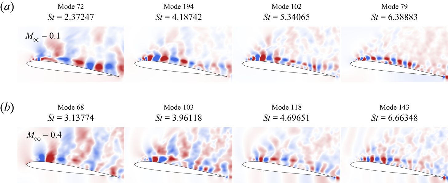
Figure 13. DMD modes for (a)  $M_{\infty } = 0.1$, and (b) $M_{\infty } = 0.4$, for the periodic motion.
The standard DMD algorithm essentially combines data from all snapshots; for example, as shown in figure 13, all modes containing coherent structure information near the leading edge also include the influence of the flow from post-stall stages. Coloured regions away from the aerofoil surface in all subplots are a remnant indication of the passage of the DSV. They arise from the fact that the extracted modes exist throughout the entire temporal window analysed, which impairs the capacity of the algorithm to highlight events that may be dominant only in a finite time window of the cycle. The signature of such events is effectively spread out over the cycle and complicates the interpretation of the DMD modes. This issue is also related to the inefficacy of SVD based approaches to extract low-rank dynamics from data with translational and rotational invariance, as discussed in the work of Kutz et al. (Reference Kutz, Fu and Brunton2016), where the mrDMD algorithm is proposed.
Despite these limitations, some useful observations can still be drawn from these modes. For instance, the intense structures close to the aerofoil surface, especially around the leading edge region, are shifted slightly downstream for the  $M_{\infty } = 0.4$ case. The results also suggest that the frequencies of the structures associated with dynamic stall onset between the two Mach number flows are similar and range from $St \sim 1$ to $St \sim 40$. In figure 13, only a few modes are shown, so it does not cover all frequencies mentioned in that range. Moreover, these values are not precise as they are derived from a nonlinear collection of snapshots, and provide only a perception of the order of magnitude of the frequencies at play during the dynamic stall onset. The persistence of the flow structures and their corresponding frequencies across the compressible regimes investigated indicate a possible correlation of mode shapes from a parametric modal decomposition perspective, as reported by Coleman et al. (Reference Coleman, Thomas, Gordeyev and Corke2019).
The limitations of the standard DMD are now lifted by applying the mrDMD algorithm proposed by Kutz et al. (Reference Kutz, Fu and Brunton2016). Using the same procedure as before and the binning technique of § 2.3, some of the most interesting modes are presented in figure 14. In the multi-resolution approach, the modes are no longer ranked by their amplitude so that, instead of showing the index of a given mode, it is more suitable to discuss the resolution level and the bin where it resides. For clarity, the levels and bins are converted into their equivalent time periods  ${\rm \Delta} t$ and the modes are judiciously organized in the figure so that the same period of time is assimilated between the two different Mach number flows.
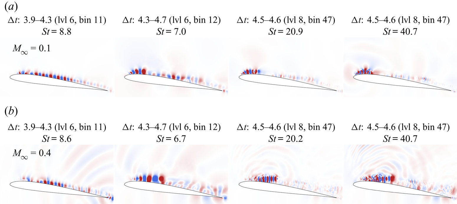
Figure 14. DMD modes obtained from the mrDMD algorithm for (a)  $M_{\infty } = 0.1$, and (b) $M_{\infty } = 0.4$, for the periodic motion.
Comparing figures 13 and 14, it is evident that the multi-resolution variant has a better capability to deal with the transient nature of dynamic stall and is able to extract clean and physically interpretable modes. Starting from the leftmost column of figure 14, we observe the structures that represent the Kelvin–Helmholtz instability formed along the aerofoil suction side. Note that the time period encompassed by this mode coincides with the time window when the instability develops, as shown in figure 4 and also the pressure gradient plot of figure 9. For the  $M_{\infty } = 0.4$ case, acoustic waves are also seen propagating from the trailing edge due to a scattering mechanism, but these are not visible for the $M_{\infty } = 0.1$ case since the acoustic waves have a lower amplitude for this flow. The spatial distribution of the modes is also different. While a quasi-continuous train of Kelvin–Helmholtz disturbances appears as a wavepacket at $M_{\infty } = 0.1$, the structures are more sparsely distributed for $M_{\infty } = 0.4$, being more concentrated at the mid-chord. This is consistent with the observation of high frequency oscillations in the skin friction and pressure gradient maps of figures 3 and 9, respectively. It is also interesting to note that the frequencies between the two compressible cases are much alike, and this holds for all subplots.
The modes depicted in the subsequent columns of figure 14 are associated with the growth of the shear layer instabilities close to the leading edge and the separation process that leads to the formation of the DSV. In the second column, the modes represent the advection of vortical structures formed in the leading edge shear layer instability, which coalesce afterwards to form the DSV. Finally, the last two columns refer to the same time period and mark the separation process described earlier, in figures 5 and 6, where nonlinear mechanisms govern the evolution of the flow. As indicated in figure 14, the frequencies increase substantially at this stage, independently of the Mach number. While the structures observed in the last two columns are more organized and compact for  $M_{\infty } = 0.1$, those appearing in the $M_{\infty } = 0.4$ flow are composed of a wider range of spatial scales. This observation may reflect the higher three-dimensionality of the $M_{\infty } = 0.4$ flow, as shown in figure 10. As discussed before, the structures are also formed downstream for the $M_{\infty } = 0.4$ case and extend over a larger portion of the aerofoil chord. For these DMD modes, one can also see that acoustic waves are generated by the hydrodynamic fluctuations near the leading edge. These waves have higher wavenumbers for the $M_{\infty } = 0.4$ flow and may contribute to the earlier breakdown into three-dimensional structures.
4. Conclusions
Large eddy simulations are performed to investigate the onset and evolution of dynamic stall for an SD7003 aerofoil undergoing a periodic plunging motion. Simulations are performed for freestream Mach numbers  $M_{\infty } = 0.1$ and $0.4$ for a fixed-chord-based Reynolds number $Re=6\times 10^{4}$ to examine phenomenological variations due to compressibility effects. Similar to previous observations reported for pitching aerofoils, it is found that both the residence time and strength of the dynamic stall vortex (DSV) decrease for the higher Mach number flow. Hence higher compressibility leads to lift and drag reductions caused by the weakened DSV, which occurs when the aerofoil is ceasing its downstroke motion. For the rest of the periodic motion, the aerodynamic coefficients display similar features at both Mach numbers.
For the present configurations, the onset of dynamic stall is marked by two major flow features: a train of Kelvin–Helmholtz instabilities, referred to here as the primary instability stage, and a secondary instability stage due to the breakdown of vortical structures along a shear layer formed at the leading edge. With respect to the primary stage, acoustic waves are scattered from the trailing edge due to vortex shedding apparently triggering the formation of Kelvin–Helmholtz instabilities. This mechanism appears to be invariant to the freestream Mach number although it is observed that higher compressibility induces the flow to become more susceptible to three-dimensional spanwise disturbances.
With respect to the secondary stage of instabilities, the mechanisms of flow separation observed in the present plunging aerofoil display broad agreement with the van Dommelen and Shen model for pitching aerofoils. In this case, complex dynamics are observed along a shear layer formed at the leading edge. The evolution of this shear layer causes the flow to eject vortical structures outwards from the surface. The flow dynamics are similar for both Mach numbers analysed, despite the different positions where they occur near the leading edge. These spatial variations are affected directly by the pressure gradient distributions over the leading edge. For  $M_{\infty }=0.1$, the pressure gradient becomes adverse sooner than for $M_{\infty }=0.4$, and the pressure gradient fluctuations are stronger, causing the shear layer to destabilize further upstream. We observe that the onset of dynamic stall is related to the interaction of both primary and secondary instabilities that occur near the leading edge.
In order to better characterize the stall onset, two empirical indicators are investigated: the leading edge suction parameter (LESP) and the critical chord-normal shear layer height,  ${\rm \Delta} z$. The influence of compressibility on these stall indicators is also assessed. It is observed that the maximum suction supported by the leading edge is reduced as compressibility increases, revealing that the LESP is a function of not only the parameters of the aerofoil motion but also the freestream Mach number. The ${\rm \Delta} z$ criterion, on the other hand, appears to be almost invariant to the freestream Mach number. We also find that although both criteria fit the observable moment when the DSV forms, they tend to characterize the stall onset based on the point when the DSV detaches from the aerofoil surface, and not when the secondary instabilities set in. From the perspective of dynamic stall control, this fact reveals the need to create more conservative criteria to predict stall. This is necessary since flow actuation should be applied prior to the formation of the DSV.
A decomposition of the pressure coefficient field into dynamic modes is also performed to extract the low-rank spatial features from the datasets and their associated frequencies. The detailed description of the boundary layer state with the modal support can help the exploration of suitable actuation parameters for flow control. The standard DMD algorithm is able to identify the modes associated with the periodic motion and its harmonics; however, it fails to isolate the unsteady flow features that take place during the onset of dynamic stall. This limitation arises from the fact that the extracted modes exist throughout the entire temporal window analysed. The multi-resolution variant of the algorithm (mrDMD), on the other hand, successfully extracts clean and physically interpretable modes for all cases investigated herein.
Although the spatial distribution of the modes related to the dynamic stall onset may vary with compressibility, their frequency contents are much alike. The mrDMD captures the wavepacket structure of the Kelvin–Helmholtz instability and the modes associated to the separation process that lead to the formation of the leading edge vortex. The effects of increasing compressibility are also manifested in these modes. For instance, the sparser distribution of Kelvin–Helmholtz instabilities, the larger size of the secondary separation in the shear layer, and the displacement of the critical region further downstream of the leading edge, which occur when the Mach number increases, are all represented therein.
Supplementary movies
Supplementary movies are available at https://doi.org/10.1017/jfm.2022.165.
Acknowledgements
The authors thank the Ohio Supercomputer Center (OSC), CEPID-CeMEAI cluster Euler, and cluster SDumont (Project SimTurb) for providing the computational resources for this research.
Funding
The authors acknowledge Fundação de Amparo à Pesquisa do Estado de São Paulo (FAPESP) for supporting this research under grant nos 2013/07375-0, 2017/10795-1, 2019/02335-6 and 2021/06448-0, and Conselho Nacional de Desenvolvimento Científico e Tecnológico (CNPq) for supporting this research under grant nos 407842/2018-7 and 304335/2018-5.
Declaration of interests
The authors report no conflict of interest.
Appendix A. Dynamic mode decomposition algorithm
In this appendix, we provide more details about the DMD algorithm. It proceeds as follows.
(1) The snapshots are stored columnwise in two separate matrices $\boldsymbol {X}$ and $\boldsymbol {X}'$ in $\mathbb {C}^{m \times n-1}$ such that
(A1a,b)where\begin{equation} \boldsymbol{X} = \left[ \begin{array}{@{}cccc@{}} | & | & & | \\ \boldsymbol{x}_{1} & \boldsymbol{x}_{2} & \ldots & \boldsymbol{x}_{n-1} \\ | & | & & | \end{array} \right] \quad \text{and} \quad \boldsymbol{X}' = \left[ \begin{array}{@{}cccc@{}} | & | & & | \\ \boldsymbol{x}_{2} & \boldsymbol{x}_{3} & \ldots & \boldsymbol{x}_{n} \\ | & | & & | \end{array} \right], \end{equation}$\boldsymbol {x}_{i}$, for $i = 1, 2, 3,\ldots,n$, represents the $i$th snapshot. Here, $m$ is the number of grid points, and $n$ is the total number of snapshots.
$\boldsymbol {X}$ and $\boldsymbol {X}'$ in $\mathbb {C}^{m \times n-1}$ such that
(A1a,b)where\begin{equation} \boldsymbol{X} = \left[ \begin{array}{@{}cccc@{}} | & | & & | \\ \boldsymbol{x}_{1} & \boldsymbol{x}_{2} & \ldots & \boldsymbol{x}_{n-1} \\ | & | & & | \end{array} \right] \quad \text{and} \quad \boldsymbol{X}' = \left[ \begin{array}{@{}cccc@{}} | & | & & | \\ \boldsymbol{x}_{2} & \boldsymbol{x}_{3} & \ldots & \boldsymbol{x}_{n} \\ | & | & & | \end{array} \right], \end{equation}$\boldsymbol {x}_{i}$, for $i = 1, 2, 3,\ldots,n$, represents the $i$th snapshot. Here, $m$ is the number of grid points, and $n$ is the total number of snapshots.(2) The SVD of
$\boldsymbol {X}$ is computed to obtain a low-rank representation of the data as
(A 2)where\begin{equation} \boldsymbol{X} \approx \boldsymbol{U} \boldsymbol{\varSigma} \boldsymbol{V}^{*}, \end{equation}$\boldsymbol {U} \in \mathbb {C}^{m \times r}$, $\boldsymbol {\varSigma } \in \mathbb {C}^{r \times r}$, $\boldsymbol {V} \in \mathbb {C}^{n \times r}$, and $*$ denotes the conjugate transpose. Here, $r$ is the rank of the reduced SVD approximation to $\boldsymbol {X}$, which can be computed using the recent hard-thresholding algorithm of Gavish & Donoho (Reference Gavish and Donoho2014). The matrices $\boldsymbol {U}$ and $\boldsymbol {V}$ are named the left singular vectors and right singular vectors of $\boldsymbol {X}$, respectively, and $\boldsymbol {\varSigma }$ is a diagonal matrix containing the singular values.(3) The best-fit linear operator
$\boldsymbol {A}$ is computed to map $\boldsymbol {X}' \approx \boldsymbol {A} \boldsymbol {X}$ through a pseudo-inverse of the SVD approximation of $\boldsymbol {X}$:
(A 3)In practice, however, the operator\begin{equation} \boldsymbol{A} = \boldsymbol{X}'\boldsymbol{V}\boldsymbol{\varSigma}^{{-}1}\boldsymbol{U}^{*}. \end{equation}$\boldsymbol {A}$ can be prohibitively large for the next step of the algorithm, and a matrix similarity $\tilde {\boldsymbol {A}} = \boldsymbol {U}^{*} \boldsymbol {A} \boldsymbol {U}$, which defines a low-dimensional approximation of the linear dynamical system $\tilde {\boldsymbol {x}}_{k+1} = \tilde {\boldsymbol {A}} \tilde {\boldsymbol {x}}_k$, is used instead. In this sense, we have
(A 4)\begin{equation} \tilde{\boldsymbol{A}} = \boldsymbol{U}^{*} \boldsymbol{X}' \boldsymbol{V} \boldsymbol{\varSigma}^{{-}1} . \end{equation}(4) The eigendecomposition of
$\tilde {\boldsymbol {A}}$ is computed as
(A 5)where\begin{equation} \tilde{\boldsymbol{A}} \boldsymbol{W} = \boldsymbol{W} \boldsymbol{\varLambda}, \end{equation}$\boldsymbol {W}$ is the matrix containing the eigenvectors (stored columnwise), and $\boldsymbol {\varLambda }$ is a diagonal matrix with the corresponding eigenvalues $\lambda _k$.(5) The eigendecomposition of the original system is reconstructed using either
(A 6)or\begin{equation} \boldsymbol{\varPhi} = \boldsymbol{U} \boldsymbol{W} \quad\text{(Projected)} \end{equation}(A 7)Each eigenvector\begin{equation} \boldsymbol{\varPhi} = \boldsymbol{X}' \boldsymbol{V} \boldsymbol{\varSigma}^{{-}1} \boldsymbol{W} \quad \text{(Exact).} \end{equation}$\boldsymbol {\phi }_k$ of $\boldsymbol {\varPhi }$ represents a DMD mode. These two distinct ways to reconstruct the modes occur because Tu et al. (Reference Tu, Rowley, Luchtenburg, Brunton and Kutz2014) showed that the exact modes are the actual eigenvectors of matrix $\boldsymbol {A}$, in contrast to the original definition of Schmid (Reference Schmid2010) for the projected modes. However, they tend to converge if $\boldsymbol {X}$ and $\boldsymbol {X}'$ have the same column spaces.(6) Finally, the initial amplitudes
$b_k$ of each mode are found such that the solution is approximated by
(A 8)Here,\begin{equation} \boldsymbol{x}(t) \approx \sum_{k=1}^{r} \boldsymbol{\phi}_k \exp(\omega_k t)\,b_k = \boldsymbol{\varPhi} \exp(\boldsymbol{\varOmega} t)\,\boldsymbol{b} . \end{equation}$\omega _k = \ln (\lambda _k)/{\rm \Delta} t$, and $\boldsymbol {\varOmega }$ is a diagonal matrix whose entries are the $\omega _k$ values. There exist different ways to evaluate the initial amplitude. By considering the first snapshot at time $t_1 = 0$, which gives $\boldsymbol {x}_1 = \boldsymbol {\varPhi } \boldsymbol {b}$, one can evaluate
(A 9)where\begin{equation} \boldsymbol{b} = \boldsymbol{\varPhi}^{{{\dagger}}} \boldsymbol{x}_1, \end{equation}${\dagger}$ stands for the Moore–Penrose pseudo-inverse. Following Tu et al. (Reference Tu, Rowley, Luchtenburg, Brunton and Kutz2014), it is possible to use the principal component (POD) subspace to determine $\boldsymbol {b}$ through less expensive computations as
(A 10)where\begin{equation} \boldsymbol{b} \approx (\boldsymbol{W} \boldsymbol{\varLambda})^{{-}1} \boldsymbol{\alpha}_1, \end{equation}$\boldsymbol {\alpha }_1$ is obtained from the matrix product $\boldsymbol {\varSigma } \boldsymbol {V}^{*}$ associated with the first snapshot, i.e. $\boldsymbol {x}_1 \approx \boldsymbol {U} \boldsymbol {\varSigma } \boldsymbol {V}^{*} = \boldsymbol {U} \boldsymbol {\alpha }_1$. As proposed by Jovanović, Schmid & Nichols (Reference Jovanović, Schmid and Nichols2014), another possibility to calculate $\boldsymbol {b}$ is given by
(A 11)where, in this case,\begin{equation} \boldsymbol{b} = [ (\boldsymbol{W}^{*} \boldsymbol{W}) \circ \overline{(\boldsymbol{V}_{and} \boldsymbol{V}_{and}^{*} )}]^{{-}1} \overline{\text{diag}(\boldsymbol{V}_{and} \boldsymbol{V} \boldsymbol{\varSigma}^{*} \boldsymbol{W}) }, \end{equation}$*$ denotes the self-adjoint (Hermitian) operator while the overline is the complex conjugate. The symbol $\circ$ represents elementwise multiplication, and $\boldsymbol {V}_{and}$ is the Vandermonde eigenvalue matrix.


Appendix B. Harmonics of the periodic motion
In this appendix, we demonstrate that when ranked by their amplitudes, the first modes exhibit frequencies that may be associated with the harmonics of the imposed motion. Similar observations were also made by Dunne et al. (Reference Dunne, Schmid and McKeon2016) and Mohan et al. (Reference Mohan, Gaitonde and Visbal2016). Within a time period  ${\rm \pi} /k$, corresponding to a full cycle of the aerofoil motion, where $k \triangleq {\rm \pi}f c / U_{\infty } = 0.25$ is the reduced frequency, we define the Strouhal number based on the non-dimensional aerofoil chord ( $c=1$) as $St \triangleq f c / U_{\infty } = k / {\rm \pi}\approx 0.07958$. This non-dimensional frequency of the plunging motion matches that of the dominant (first) dynamic mode, which is plotted in figure 15 along with the extracted frequencies from DMD. In this figure, the modes corresponding to the harmonics of $St = 0.07958$ are also included for both Mach numbers, and the saturation levels are kept the same for all subplots, ranging from $-0.004$ to 0.004. The DMD is computed here using snapshots of the pressure coefficient.
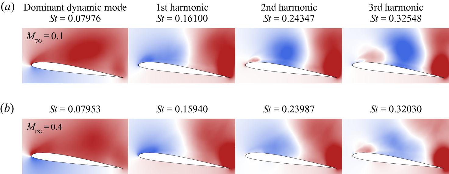
Figure 15. DMD dominant mode and subharmonics for (a)  $M_{\infty } = 0.1$, and (b) $M_{\infty } = 0.4$, for the periodic motion.
Comparing the different Mach number solutions in figure 15, a striking resemblance to the dominant dynamic mode and its harmonics is noted. This occurs because these modes are related to the aerofoil kinematics, which is the same for both Mach numbers investigated. Nevertheless, some characteristics of the higher Mach number flow are still visible in these modes, such as the weaker DSV strength. For instance, the harmonics of the  $M_{\infty } = 0.4$ flow have a slightly smaller area in blue, and the levels in these regions are reduced when compared to the $M_{\infty } = 0.1$ case. Inspection of the third harmonic for both Mach numbers shows a weaker presence of the leading edge red structure for $M_{\infty } = 0.4$; this indicates that the leading edge dynamics occurs with a different phase compared to that of the $M_{\infty } = 0.1$ case. Overall, at higher harmonics, the disparities caused by the phase lag between the two flows become more accentuated. The cause of this phase variation is the different gestation period and residency time of the DSV over the aerofoil between the two Mach number flows.


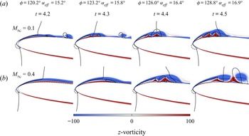


 Open access