


1. Introduction
Over erodible deposits, intermittent granular avalanches may entrain grains from the substrate, transport them downslope, and detrain them to form new deposits. Such processes occur down natural inclines such as scree slopes and dune faces, and in laboratory configurations such as slowly rotating drums and grain piles driven by low inflow (Evesque Reference Evesque1991; Arran & Vriend Reference Arran and Vriend2018). Challenges are then to determine how rates of entrainment and detrainment are set, and how these affect flow acceleration and deceleration (Iverson & Ouyang Reference Iverson and Ouyang2015; Lusso et al. Reference Lusso, Bouchut, Ern and Mangeney2021; Pudasaini & Krautblatter Reference Pudasaini and Krautblatter2021). In narrow channels, wall friction is known to be an effective mechanism to limit erosion at the base of granular avalanches (Taberlet et al. Reference Taberlet, Richard, Valance, Losert, Pasini, Jenkins and Delannay2003; Jop, Forterre & Pouliquen Reference Jop, Forterre and Pouliquen2005). A rigid floor at some depth is of course another possible constraint (Silbert et al. Reference Silbert, Ertaz, Grest, Halsey, Levine and Plimpton2001; Parez, Aharonov & Toussaint Reference Parez, Aharonov and Toussaint2016). This cannot be the whole story, however, as limits to downward erosion appear to exist even in the absence of rigid lateral or lower boundaries. In this paper, the role of bed resistance to erosion is examined. Taking this role into account, new basal boundary conditions are proposed, as needed by depth-averaged and continuum models of granular avalanches over erodible beds.
Depth-integrated and continuum models were first applied to granular avalanches over rigid boundaries (Savage & Hutter Reference Savage and Hutter1991; Silbert et al. Reference Silbert, Ertaz, Grest, Halsey, Levine and Plimpton2001). For erodible beds, the position of the basal interface becomes an additional degree of freedom (Capart, Hung & Stark Reference Capart, Hung and Stark2015; Iverson & Ouyang Reference Iverson and Ouyang2015; Lusso et al. Reference Lusso, Bouchut, Ern and Mangeney2021). To model the resulting dynamics, various approaches have been adopted. Phenomenological laws for the rate of erosion or deposition have been proposed by Bouchaud et al. (Reference Bouchaud, Cates, Ravi Prakash and Edwards1994), Tai & Kuo (Reference Tai and Kuo2008) and Lê & Pitman (Reference Lê and Pitman2010). Such laws can also be derived from the balance of momentum assuming jumps in velocity (Pudasaini & Krautblatter Reference Pudasaini and Krautblatter2021) as well as shear stress (Fraccarollo & Capart Reference Fraccarollo and Capart2002; Iverson & Ouyang Reference Iverson and Ouyang2015) or particle pressure (Jenkins & Berzi Reference Jenkins and Berzi2016) across the basal interface. Other authors have instead constrained the velocity profile during the entrainment or detrainment process. Douady, Andreotti & Daerr (Reference Douady, Andreotti and Daerr1999) and Khakhar et al. (Reference Khakhar, Orpe, Andresén and Ottino2001) assumed a constant shear rate, while Capart et al. (Reference Capart, Hung and Stark2015) and Larcher, Prati & Fraccarollo (Reference Larcher, Prati and Fraccarollo2018) let the unsteady velocity profile retain the same shape as in steady equilibrium flows. Numerical simulations, on the other hand, have shown that assumptions regarding granular stresses suffice to model the unsteady evolution of eroding (Jop, Forterre & Pouliquen Reference Jop, Forterre and Pouliquen2007) and detraining flows (Barker & Gray Reference Barker and Gray2017). To model these stresses, previous authors have used the  $\mu (I)$ rheology (Jop et al. Reference Jop, Forterre and Pouliquen2007; Ionescu et al. Reference Ionescu, Mangeney, Bouchut and Roche2015; Sarno et al. Reference Sarno, Wang, Tai, Papa, Villani and Oberlack2022), regularized and non-local versions of this rheology (Barker & Gray Reference Barker and Gray2017; Lin & Yang Reference Lin and Yang2020) and extended kinetic theory (Jenkins & Berzi Reference Jenkins and Berzi2016; Larcher et al. Reference Larcher, Prati and Fraccarollo2018).
Model predictions match unsteady flow experiments reasonably well (Jop et al. Reference Jop, Forterre and Pouliquen2007; Capart et al. Reference Capart, Hung and Stark2015; Larcher et al. Reference Larcher, Prati and Fraccarollo2018). To complicate matters, however, experiments initiated from inclined granular beds at rest exhibit two distinct behaviours. In some experiments (Jop et al. Reference Jop, Forterre and Pouliquen2007; Capart et al. Reference Capart, Hung and Stark2015), flows instantaneously mobilize a layer of finite thickness, whereas in others (Larcher et al. Reference Larcher, Prati and Fraccarollo2018), the flow thickness grows gradually from zero. Some models (Jop et al. Reference Jop, Forterre and Pouliquen2007; Capart et al. Reference Capart, Hung and Stark2015) describe well the abrupt start observed in the first experiments, while others (Jenkins & Berzi Reference Jenkins and Berzi2016; Larcher et al. Reference Larcher, Prati and Fraccarollo2018) predict a gradual growth as observed in the second experiments. To model these distinct behaviours, it is proposed in this paper that bed resistance to erosion must be taken into account. Depending on how granular beds are prepared, two situations are considered. In the first, the bed offers the same resistance to erosion as grains do to sustained shear. This is expected, for instance, for beds produced by gently arresting sustained granular shear flows, as in the experiments of Capart et al. (Reference Capart, Hung and Stark2015). Berzi, Jenkins & Richard (Reference Berzi, Jenkins and Richard2019) have characterized such beds in detail using discrete element simulations, and refer to them as fragile. In the second situation, the bed offers an excess resistance to erosion, and the basal shear stress needed to produce erosion is greater than the shear stress needed to sustain shear. This is expected when granular beds have been subjected to some compaction, say due to lid pressure applied before release as in the experiments of Larcher et al. (Reference Larcher, Prati and Fraccarollo2018), or due to prior burial as in rotating drum experiments (Evesque Reference Evesque1991). By analogy with the terminology used for slopes (Bishop Reference Bishop1971), such beds will be referred to as brittle.
To model the contrasted responses of fragile and brittle beds, a distinction must be drawn between resistance to erosion and resistance to flow. This relates to that observed, in shear cell or shear box tests, between peak and residual shear strengths. In laboratory shear tests conducted at very slow deformation rates, many granular materials exhibit the behaviour illustrated in figure 1(a): as the shear deformation  $\gamma$ increases, the ratio of applied shear to normal stress $\tau /\sigma$ rises first to a peak value, $\tan \varphi _{ p}$, before decreasing to an asymptotic residual value, $\tan \varphi _c$, where $\varphi _c$ is called the critical angle. Although the peak value depends on how grains interlock prior to deformation, the residual or critical value is a material property that doesn't depend on how the sample was prepared. This difference between peak and residual shear strengths, and the shear weakening behaviour that occurs after the peak strength has been reached, matter greatly to geotechnical engineers, as they control the brittleness of slope failures (Bishop Reference Bishop1971; Soga et al. Reference Soga, Alonso, Yerro, Kumar and Bandara2016; Yerro, Alonso & Pinyola Reference Yerro, Alonso and Pinyola2016). They have also been hypothesized to control intermittent granular avalanching in slowly rotating drums (Evesque Reference Evesque1991; Marteau & Andrade Reference Marteau and Andrade2018).

Figure 1. Definition sketch: (a) typical shear test curve with peak and residual strengths; (b) idealized response assumed at interface between granular flow and erodible bed when  $\gamma \gg \gamma _c$; (c) assumed flow geometry and kinematics.
Bed resistance to erosion, however, should not simply be equated to the peak shear resistance observed in shear box or shear cell tests. This is because, in such tests, the failure surface cuts through an assembly of interlocking grains. At the interface between granular flow and erodible bed, by contrast, the interface features interlocking grains to one side only. Resistance to erosion, therefore, will be described by a shear strength  $\tau _e$ intermediate between the critical and peak strengths. As described below, this is needed also to ensure the stability of the underlying bed. As illustrated by figure 1(a), geotechnical shear tests typically measure some finite shear deformation, $\gamma _{ p}$, before granular materials develop their peak resistance, then some further deformation, $\gamma _c$, before they degrade to their residual resistance. In the context of flows that rapidly attain very large deformations, resistance to erosion will be further idealized as illustrated in figure 1(b): to initiate erosion, the excess resistance $\tau _e = \tan \varphi _{ e} \,\sigma$ must be overcome, but the resistance to sustained shear drops immediately to the critical shear strength $\tau _c = \tan \varphi _c \,\sigma$.
In the present work, this idealized behaviour will be incorporated into new basal boundary conditions for granular surface flows. To make the approach work, it is necessary to specify exactly how the different variables behave at the base, not just when entrainment occurs, but also when the flow thickness stays the same, or when the flow layer thins by detraining grains back to the substrate. The rate of entrainment or detrainment, moreover, must also be determined by the theory. The unsteady velocity profile, finally, must be allowed to evolve freely. The principal objective of this work is to propose new basal boundary conditions that meet these requirements. After formulating these basal boundary conditions, their consequences will be examined in what may be the simplest possible configuration: the surface flow of grains in a long channel of adjustable inclination (figure 1c). In this configuration, flows can be idealized as uniform in both longitudinal and transverse directions, and the longitudinal flow velocity  $u$ becomes a function of only two variables: the depth $y$ and the elapsed time $t$. With these simplifications, our goal will be to determine the flow thickness $h(t)$ and velocity profile $u(y,t)$ for three cases: stationary flows; starting; and stopping transients. Although such conditions have been considered earlier (Jop et al. Reference Jop, Forterre and Pouliquen2007; Capart et al. Reference Capart, Hung and Stark2015; Parez et al. Reference Parez, Aharonov and Toussaint2016; Barker & Gray Reference Barker and Gray2017), new to this work will be the distinctive flow behaviours that result when beds offer an excess resistance to erosion.
2. Governing equations and constitutive assumptions
As illustrated by figure 1(c), consider a channel of constant width  $W$ and possibly time-evolving inclination angle $\theta (t)$, filled with a uniform, dry, static layer of granular material. The depth coordinate $y$ is taken normal to the free surface, setting $y=0$ at the free surface and $y$ positive going down. By inclining the channel, a shear flow of finite thickness can be produced, below which the granular substrate remains static. This flow may or may not reach a stationary state, before the channel inclination is reduced and the flow brought back to a stop. The flow may also be constrained by a rough, rigid floor at depth $y = H$. For simplicity, variations across the width and along the length of the channel are neglected. Our objective is then to determine the time-dependent flow thickness $h(t)$ and velocity profile $u(y,t)$.
Under these assumptions, momentum balance equations in the longitudinal and normal directions can be written as
 \begin{equation} \rho \frac{\partial{u}}{\partial{t}} = \rho g_{_\perp} \tan \theta - 2\frac{\tau_w}{W} -\frac{\partial{\tau}}{\partial{y}} \quad \text{and} \quad \frac{\partial{\sigma}}{\partial{y}} = \rho g_{_\perp}, \end{equation}
where  $\rho$ is the bulk density, $g_{_\perp } = g \cos \theta$ is the normal component of the gravitational acceleration, $\tau _w$ is the shear stress along the walls, $\tau$ is the internal shear stress and $\sigma$ is the normal stress. In the flowing layer ( $0 \leq y \leq h(t)$), where grains slide along the walls and undergo sustained shear, constitutive relations are provided as follows. For the wall shear stress, the Coulomb friction law $\tau _w = \mu _w \sigma$ is adopted, where $\mu _w$ is a constant grain–wall friction coefficient (Jop et al. Reference Jop, Forterre and Pouliquen2005). For the internal shear stress, the linearized $\mu (I)$ rheology is assumed (da Cruz et al. Reference da Cruz, Emam, Prochnow, Roux and Chevoir2005; Jop et al. Reference Jop, Forterre and Pouliquen2005), whereby
 \begin{equation} \tau = \tan \varphi_c\,\sigma + \chi D (\rho\sigma)^{1/2}\dot{\gamma}. \end{equation}
Here  $\dot {\gamma } = -\partial u/\partial y$ is the shear rate, $\tan \varphi _{{c}}$ is the residual or critical value of the coefficient of internal friction, $D$ is the grain diameter and $\chi$ is a dimensionless coefficient that sets the strength of the pressure-dependent viscosity $\chi D (\rho \sigma )^{1/2}$. This relationship is taken to hold throughout the flowing layer, including immediately above the basal interface. The excess resistance to erosion $\tau _e = \tan \varphi _e \,\sigma$ applies below this interface, to the top of the static bed. The corresponding basal boundary condition is described in the next section.
To close the description, boundary conditions must be provided along the free surface,  ${\widetilde {y}} = 0$, and along the basal interface ${{y}\unicode{x0330}} = h(t)$. Here tildes over and below variables will be used to denote variables sampled at the free surface and basal interface, respectively. Along the free surface, stress-free boundary conditions can be written $\widetilde {\tau } = \widetilde {\sigma } = 0$, so that integrating down from the free surface yields the lithostatic normal stress profile $\sigma (y,t) = \rho g_{_\perp } y$, and the basal normal stress ${{\sigma}\unicode{x0330}} = \rho g _{_\perp} h$.
Up to this point, it is largely agreed that the above equations closely approximate the behaviour of many granular surface flows. Possibly with minor variations, this description has been applied to a variety of parallel flows and found to closely match discrete element simulations (da Cruz et al. Reference da Cruz, Emam, Prochnow, Roux and Chevoir2005; Parez et al. Reference Parez, Aharonov and Toussaint2016) and laboratory experiments (Berzi & Jenkins Reference Berzi and Jenkins2008; Capart et al. Reference Capart, Hung and Stark2015). Regarding basal boundary conditions for flows over erodible substrates, however, there is less consensus (Iverson & Ouyang Reference Iverson and Ouyang2015; Lusso et al. Reference Lusso, Bouchut, Ern and Mangeney2021; Pudasaini & Krautblatter Reference Pudasaini and Krautblatter2021). What is needed is to specify boundary conditions for the flow velocity  ${{u}\unicode{x0330}}$, shear rate ${\dot{\gamma}\unicode{x0330}}$ and/or shear stress ${\tau \unicode{x0330}}$ at the base, so that the flow thickness $h$ or its evolution over time $h(t)$ can also be determined. In the next section, a new formulation is proposed, applicable also to granular substrates that offer an excess resistance to erosion.
3. Basal boundary conditions
When granular shear flows reach down to a rough, rigid floor at depth  ${{y}\unicode{x0330}}=H$, the simplest assumption is to prescribe no slip along the floor, ${{u}\unicode{x0330}} = 0$, and let the basal shear rate ${\dot{\gamma}\unicode{x0330}}$ adjust freely (Silbert et al. Reference Silbert, Ertaz, Grest, Halsey, Levine and Plimpton2001; Parez et al. Reference Parez, Aharonov and Toussaint2016). For loose boundary flows over static, erodible granular substrates $(h< H)$, previous investigators (Berzi & Jenkins Reference Berzi and Jenkins2008; Capart et al. Reference Capart, Hung and Stark2015) added the condition that
 \begin{equation} {\dot{\gamma}\unicode{x0330}}{(t)} = \dot{\gamma}(h(t){,t}) = 0, \end{equation}
i.e. the basal shear rate must also vanish. This is consistent with plastic yield at the base, assuming no excess resistance to erosion. When there is such an excess resistance, the proposal here is to write conditions that transition between rigid-like and loose cases, dependent on whether the flow thickens, thins or maintains a constant thickness. To distinguish between these cases, it is useful to express the rate of change of the flow thickness in the form
 \begin{equation} \frac{\mathrm{d} h}{\mathrm{d} t} = e - d, \end{equation}
where  $e(t) \geq 0$ and $d(t) \geq 0$ are, respectively, rates of entrainment (erosion) and detrainment (deposition), assumed positive and subject to the complementarity condition $e d = 0$ so that at most one process (entrainment or detrainment) is active at any given time. Depending on the case, the following assumptions are proposed. For the flow to entrain ( $e>0$, $d=0$), the shear stress $\tau{\unicode{x0330}}$ exerted by the flowing layer on the granular substrate must attain the erosion resistance of this substrate, $\tau _{{e}} = \tan \varphi _{{e}} \sigma$, hence
 \begin{equation} {\tau}\unicode{x0330} = \tan \varphi_{{c}}\,{\sigma}\unicode{x0330} + \chi D (\rho {\sigma}\unicode{x0330})^{1/2}\,{\dot{\gamma}\unicode{x0330}} = \tan \varphi_{{e}}\,{\sigma}\unicode{x0330}. \end{equation}
The value  ${\dot{\gamma}\unicode{x0330}}$ that satisfies this condition,
 \begin{equation} {\dot{\gamma}\unicode{x0330}} = {\dot{\gamma}\unicode{x0330}}_{max} = \frac{\tan \varphi_{{e}}-\tan \varphi_{{c}}}{\chi D}\left(\frac{{\sigma}\unicode{x0330}}{\rho}\right)^{ 1/2} = \frac{\tan \varphi_{{e}}-\tan \varphi_{{c}}}{\chi D} (g_{_\perp} h)^{1/2}, \end{equation}
represents a maximum value for the basal shear rate. When this value is reached, the flow evolves by eroding substrate grains instead of further increasing its basal shear rate. Conversely, for the flow to detrain ( $e=0$, $d>0$), the shear rate at the base must first drop to zero, ${\dot{\gamma}\unicode{x0330}} = {\dot{\gamma}\unicode{x0330}}_{min} = 0$, which represents a minimum value for the basal shear rate. When this value is reached, the flow evolves by depositing static grains back to the substrate, for otherwise a negative shear rate combined with the no slip basal boundary condition would imply unphysical negative velocities. Across the basal interface, note that the shear rate can be discontinuous, but the velocity and stress profiles are assumed continuous.
Finally between these two values,  $0 < {\dot{\gamma}\unicode{x0330}} < {\dot{\gamma}\unicode{x0330}}_{max}$, the flow can neither entrain nor detrain, hence $e = d = 0$, a state that can be called bypass by analogy with gravity currents that neither entrain nor deposit sediment at their base (Sequeiros et al. Reference Sequeiros, Naruse, Endo, Garcia and Parker2009). When the bed is fragile and $\tan \varphi _{{e}} = \tan \varphi _{{c}}$, then ${\dot{\gamma}\unicode{x0330}}_{min} = {\dot{\gamma}\unicode{x0330}}_{max} = 0$ and the boundary condition ${\dot{\gamma}\unicode{x0330}} = 0$ assumed in previous work is recovered. When the bed is brittle and $\tan \varphi _{{e}}>\tan \varphi _{{c}}$, however, a gap opens between the two bounds, over which the flow experiences its base as rigid-like. Only when ${\dot{\gamma}\unicode{x0330}}$ attains the bounds of this interval can the transfer of grains between the flow and its substrate occur. The above physical assumptions can be summarized in compact mathematical form by the following complementary inequalities: for entrainment,
 \begin{equation} e \geq 0, \quad {\dot{\gamma}\unicode{x0330}} \leq {\dot{\gamma}\unicode{x0330}}_{max}, \quad ({\dot{\gamma}\unicode{x0330}}_{max} - {\dot{\gamma}\unicode{x0330}}) e = 0; \end{equation}
for detrainment,
 \begin{equation} d \geq 0, \quad 0 \leq {\dot{\gamma}\unicode{x0330}}, \quad {\dot{\gamma}\unicode{x0330}} d = 0. \end{equation}
In both equations, a pair of inequalities is complemented by the condition that, when one term of the product is non-zero, the other term has to be zero. Together, (3.5) and (3.6) allow granular flows over erodible substrates to transition between entrainment and bypass, and between bypass and detrainment. Complementarity formulations of this kind have been derived for many free and moving boundary problems (Elliott & Ockendon Reference Elliott and Ockendon1982; Baumgarten & Kamrin Reference Baumgarten and Kamrin2019). Together with the no slip condition, (3.5) and (3.6) form a complete set of basal boundary conditions, and represent the key novel feature of this work. Despite their simplicity, they will be shown below to produce a variety of distinctive flow behaviours.
4. Stationary solutions
To examine how flow behaviour is affected by basal boundary conditions, consider first steady flow at a constant channel inclination  $\tan \theta$. In that case, $\partial u/\partial t = 0$ and $\mathrm {d} h/\mathrm {d} t = 0$, hence $e=d=0$. Equation (2.1a,b) is then satisfied by the two-parameter family of profile shapes,
 \begin{equation} u(\eta) = \tfrac{2}{5}\left(\tfrac{2}{3} - \tfrac{5}{3}\eta^{3/2} + \eta^{5/2}\right) h \varGamma + \tfrac{2}{3}(1-\eta^{3/2})h {\dot{\gamma}\unicode{x0330}}, \end{equation}
where  $\eta = y/h$ is a dimensionless depth coordinate, and the two components are scaled by characteristic shear rates $\varGamma$ and ${\dot{\gamma}\unicode{x0330}}$. The first component, scaled by parameter $\varGamma$, coincides with Takahashi's equilibrium shape for debris flows over erodible substrates, between frictional walls (Takahashi Reference Takahashi1991; Berzi & Jenkins Reference Berzi and Jenkins2008). The second, scaled by the basal shear rate ${\dot {\gamma}\unicode{x0330}}$, coincides with the equilibrium Bagnold profile for flows over a rigid floor, without wall friction (Silbert et al. Reference Silbert, Ertaz, Grest, Halsey, Levine and Plimpton2001). Equilibrium at channel inclination $\tan \theta$ further requires that
 \begin{equation} \varGamma = \frac{\mu_w g_{_\perp}^{1/2} h^{3/2}}{W \chi D} \quad \text{and} \quad {\dot{\gamma}\unicode{x0330}} = \frac{(g_{_\perp} h)^{1/2}}{\chi D} \left( \tan \theta - \tan \varphi_{{c}} - \frac{\mu_w h}{W}\right). \end{equation}
Since there are two constraints but three unknowns  $h$,
$h$,  $\varGamma$ and ${\dot{\gamma}\unicode{x0330}}$, for a given inclination $\tan \theta$ the stationary solution is not unique. Nevertheless, the range of solutions is restricted by the condition $0 \leq {\dot{\gamma}\unicode{x0330}} \leq {\dot{\gamma}\unicode{x0330}}_{max}$. Unique solutions are obtained at both ends of this interval, associated with flows that have reached equilibrium by entraining ( $\mathrm {d} h/\mathrm {d} t>0$) or by detraining ( $\mathrm {d} h/\mathrm {d} t<0)$. If ${\dot{\gamma}\unicode{x0330}} = {\dot{\gamma}\unicode{x0330}}_{max}$ (entrainment locus), then $h = h_e(\tan \theta ) = (\tan \theta - \tan \varphi _{{e}})W/\mu _w$. If on the other hand ${\dot{\gamma}\unicode{x0330}} = 0$ (detrainment locus), then $h = h_{{c}}(\tan \theta ) = (\tan \theta - \tan \varphi _{{c}})W/\mu _w$. The only difference between the two loci is whether they involve the friction angle associated with erosion resistance, $\varphi _e$, or the critical friction angle $\varphi _c$. Between the two limits, any flow thickness in the range $h_e \leq h \leq h_{{c}}$ produces a valid stationary velocity profile, obtained by substituting $h$ into (4.2a,b) to get $\varGamma$ and ${\dot{\gamma}\unicode{x0330}}$.
An implication is that stationary profiles may become dependent on the history of the flow. To see this, consider a diagram of flow thickness versus channel inclination. Assume that the inclination  $\tan \theta$ is varied slowly, so the flow has time to adjust to steady state. Starting from rest with $h=0$, first gradually increase $\tan \theta$ until reaching and exceeding $\tan \varphi _{{e}}$, so that flow starts and grows in thickness and velocity along the entrainment locus $h=h_e(\tan \theta )$. If at some point the channel inclination is decreased, the flow will switch to bypass: its basal shear rate will gradually decrease along a leftward path of constant $h$, until reaching the detrainment locus $h = h_{{c}}(\tan \theta )$. Further decreasing the inclination will cause the flow to detrain and slow down along this locus. Hysteretic paths can thus be produced by altering the channel inclination slowly in this way. Over long times, it is also possible that the resistance of the bed may gradually degrade, from its initial erosion resistance $\tau _e$ to the residual resistance $\tau _c$. In that case, only the critical depth $h_c$ would represent a true equilibrium thickness of the flow. Transient evolutions resulting from rapid changes in channel inclination are examined in the next section.
5. Transient solutions
5.1. Seesaw flows and series solution
To examine transient behaviour, seesaw flows produced by abruptly changing the channel inclination are considered (Capart et al. Reference Capart, Hung and Stark2015; Parez et al. Reference Parez, Aharonov and Toussaint2016). The rest or flow state just before the change can then be adopted as initial condition  $u(y,0) = u_0(y)$ and the evolution calculated taking $\tan \theta$ constant and equal to the new inclination. Solutions for such flows can be obtained analytically or numerically. Analytical solutions will be used as much as possible, as they provide greater insight. It is also possible to solve (2.1a,b) by finite differences on a staggered grid, and such numerical solutions will be used to check the analytical results.
Provided that the flow thickness  $h$ after the abrupt change remains constant (rigid floor or bypass), a linear equation for $u(\eta,t)$ is obtained, and flow evolution from arbitrary initial conditions can be described analytically by a series solution (Parez et al. Reference Parez, Aharonov and Toussaint2016). For this purpose, it is convenient to choose dimensionless variables
 \begin{equation} \hat{t} = \frac{\chi Dg_{_\perp}^{1/2}}{h^{3/2}}t, \quad \hat{u} = \frac{\chi D}{|{\tan \theta-\tan \varphi_{{c}}}|g_{_\perp}^{1/2}h_{\phantom{\perp}}^{3/2}} u. \end{equation}
Equation (2.1a,b) with the  $\mu (I)$ rheology (2.2) can then be written in the dimensionless form
 \begin{equation} \frac{\partial{\hat{u}}}{\partial{\hat{t}}} ={\pm} 1 - 2\hat{\mu}_w \eta + \frac{\partial{}}{\partial{\eta}}\left(\eta^{1/2}\frac{\partial{\hat{u}}}{\partial{\eta}}\right), \end{equation}
where the plus sign applies if  $\tan \theta >\tan \varphi _c$, the minus sign if $\tan \theta <\tan \varphi _{{c}}$, and $\hat {\mu }_w = \mu _w h/(|{\tan \theta -\tan \varphi _{{c}}}|W)$ is a dimensionless wall friction coefficient. Its solution $\hat {u}(\eta,{\hat {t}}) = \hat {v}(\eta ) + \hat {w}(\eta,{\hat {t}})$ is the sum of particular and homogeneous solutions. The particular solution is
 \begin{equation} \hat{v}(\eta) ={\pm}\tfrac{2}{3}(1-\eta^{3/2}) - \tfrac{2}{5}\hat{\mu}_w(1-\eta^{5/2}), \end{equation}
in agreement with the stationary solutions of the previous section. The homogeneous solution, on the other hand, can be written as the infinite series
 \begin{equation} \hat{w}(\eta,{\hat{t}}) = \sum_{n=1}^{\infty} {\widetilde{w}}_n f_n(\eta)\exp\left(-\tfrac{9}{16}\kappa_n^2 {\hat{t}}\right). \end{equation}
Normalized so their surface velocity is equal to unity, the eigenfunctions  $f_n(\eta )$ are given by
 \begin{equation} f_n(\eta) = \varGamma(\tfrac{2}{3})(\tfrac{1}{2}\kappa_n)^{1/3}\eta^{1/4}{\rm J}_{{-}1/3}(\kappa_n\eta^{3/4}), \end{equation}
where  ${\rm J}_\nu (z)$ is the Bessel function of the first kind of order $\nu$, and $\varGamma ({\cdot })$ is the Gamma function with $\varGamma (\tfrac {2}{3})\approx 1.3541$. As needed to satisfy the no slip boundary condition, the eigenvalues $\kappa _n$ are the multiple roots of ${\rm J}_{-1/3}(z)=0$, sorted in increasing order. Finally because $\smallint _0^1 f_m(\eta )f_n(\eta )\,{\rm d}\eta = 0$ when $m \neq n$ (orthogonality property), the coefficients ${\widetilde {w}}_n$ can be calculated from the initial profile using
 \begin{equation} {\widetilde{w}}_n = \frac{\int_0^1 \left(\hat{u}_0(\eta)-\hat{v}(\eta)\right) f_n(\eta)\,{\rm d}\eta}{\int_0^1 f^2_n(\eta)\,{\rm d}\eta}. \end{equation}
For the case  $\hat {\mu }_w = 0$, an equivalent series solution was derived earlier by Parez et al. (Reference Parez, Aharonov and Toussaint2016). They did not see, however, that this solution does not apply when the flow thickness varies with time.
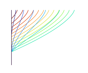
5.2. Starting transients
To illustrate flow behaviour when  $\tan \varphi _{{e}} = \tan \varphi _{{c}}$, a transient flow initiated from rest by abruptly increasing the channel inclination is shown in figure 2(a,b). To facilitate comparison, the conditions are those considered by Parez et al. (Reference Parez, Aharonov and Toussaint2016): $H= 9.6$ m; $D=H/96$; $\theta = 17 ^{\circ }$; $\mu _w = 0$; $\tan \varphi _{{c}} = 0.26$; $\chi = 1.51$. Without wall friction or excess bed resistance, the flow thickness $h(t)$ jumps abruptly to the floor-bounded thickness $H$. With wall friction, it would first jump to $h(0^+) = \tfrac {1}{2}h_{{c}}$, then gradually evolve towards $h_{{c}}=(\tan \theta -\tan \varphi _{{c}})W/\mu _w$ (Capart et al. Reference Capart, Hung and Stark2015), unless the rigid floor is first reached at depth H. When the flow starts from rest and its thickness immediately jumps to $h(0^+) = H$, the predicted evolution is simply a gradual acceleration towards the steady profile associated with the particular solution (5.3). For comparison, figure 2(a) shows the velocity profiles obtained by Parez et al. (Reference Parez, Aharonov and Toussaint2016) using the discrete element method (DEM). The evolution of velocity with time at selected depths is also shown in figure 2(b). The analytical series solution obtained for this case is identical to that of Parez et al., and in good agreement with their discrete particle simulations. In figure 2(a,b), the numerical results obtained by discretizing (2.1a,b) on a staggered grid are also shown, and checked to agree closely with the analytical results.

Figure 2. Influence of basal boundary conditions on transient flows: (a,b) starting transient,  $\tan \varphi _{{e}} = \tan \varphi _{{c}}$; (c,d) starting transient, $\tan \varphi _{{e}} > \tan \varphi _{{c}}$; (e, f) stopping transient; (a,c,e) velocity profiles at selected times; (b,d, f) velocity evolution at the selected depths indicated on panel ( f) (lines, analytical solutions; dots, numerical solutions; circles, DEM results (Parez et al. Reference Parez, Aharonov and Toussaint2016)).
The very different response obtained when  $\tan \varphi _{{e}} > \tan \varphi _{{c}}$ can now be examined. In this case, the thickness $h(t)$ no longer jumps discontinuously upon starting the flow from rest. The problem becomes a moving boundary problem ( $\mathrm {d} h/\mathrm {d} t = e > 0$), for which the series solution approach no longer works. The continuous flow thickness evolution $h(t)$, moreover, must be determined as part of the solution. Because $h(t)$ is not known in advance, a different choice of dimensionless variables must be made,
 \begin{equation} t' = \frac{g_{_\perp}^{1/2}}{(\chi D)^{1/2}} t, \quad y' = \frac{y}{\chi D}\,, \quad h' = \frac{h}{\chi D}, \quad u' = \frac{u}{(\tan \varphi_{{e}}-\tan \varphi_{{c}})g_{_\perp}^{1/2}(\chi D)^{1/2}}, \end{equation}
yielding instead of (5.2) the alternative dimensionless form,
 \begin{equation} \frac{\partial u'}{\partial t'} = S' - 2\mu'_w y' + \frac{\partial }{\partial y'}\left(y'^{1/2} \frac{\partial u'}{\partial y'} \right), \end{equation}
where  $\mu '_w = \mu _w \chi D/((\tan \varphi _{{e}}-\tan \varphi _{{c}})W)$, and $S' = (\tan \theta - \tan \varphi _{{c}})/(\tan \varphi _{{e}}-\tan \varphi _{{c}})$ is a dimensionless excess inclination. Because flows started from rest must entrain grains from the substrate, the applicable basal boundary conditions are, in dimensionless form,
 \begin{equation} u'(h'(t'),t') = 0, \quad \text{and} \quad {\frac{\partial{u'}}{\partial{y'}}(h'(t'),t') ={-}h_{\phantom{1}}^{\prime} (t')^{1/2}}. \end{equation}
No general solution can be found to this moving boundary problem. When there is no wall friction, however, a similarity solution of the form
 \begin{equation} u'(y',t') = F(\eta)\, t'^{\alpha}, \quad h'(t') = \lambda\,t'^{\beta}, \end{equation}
can be sought. Here  $\eta (y',t')=y'/h'(t')$ is the similarity variable, $\alpha, \beta$ unknown exponents, $F(\eta )$ an unknown function and $\lambda$ an unknown parameter. Using the chain rule, it follows that
 \begin{gather} \frac{\partial u'}{\partial t'} = \alpha t'^{\alpha-1} F(\eta) - \beta t'^{\alpha-1}\eta \frac{\mathrm{d} F}{\mathrm{d} \eta}, \end{gather}
 \begin{gather} \frac{\partial}{\partial y'}\left(y'^{1/2} \frac{\partial u'}{\partial y'} \right) = \frac{t'^{\alpha-3\beta/2}}{\lambda^{3/2}}\frac{\mathrm{d}}{\mathrm{d} \eta}\left( \eta^{1/2}\frac{\mathrm{d} F}{\mathrm{d} \eta} \right). \end{gather}
Substituting into (5.8) and taking  $\mu '_w = 0$, the time variable $t'$ can be eliminated from the equation by choosing for the similarity exponents the values $\alpha =1$ and $\beta =\tfrac {2}{3}$. The partial differential equation (5.8) then reduces to the second-order linear ordinary differential equation
 \begin{equation} F(\eta) - \frac{2}{3} \eta \frac{{\rm d}F}{{\rm d}\eta} - \frac{1}{\lambda^{3/2}} \frac{{\rm d}}{{\rm d}\eta}\left( \eta^{1/2} \frac{{\rm d}F}{{\rm d}\eta} \right) = S'. \end{equation}
A particular solution is obviously the constant function  $f(\eta ) = S'$. For the homogenous equation, a solution of the form $g(\eta ) = 1 + a\eta ^b$ can be tried, with $a, b$ yet to be determined. Substitution into (5.13) yields the algebraic equation
 \begin{equation} 1 + a \eta^b - \frac{2}{3} a b \eta^b - \frac{1}{\lambda^{3/2}} a b\left(b-\frac{1}{2}\right)\eta^{b-3/2} = 0, \end{equation}
which requires  $b = \tfrac {3}{2}$ and $a = \tfrac {2}{3} \lambda ^{3/2}$. The combination $F(\eta ) = f(\eta ) + cg(\eta )$ that satisfies the no slip boundary condition $F(1) = 0$ at the base is then given by
 \begin{equation} F(\eta) = \frac{\lambda^{3/2}}{\tfrac{3}{2}+\lambda^{3/2}}S'(1-\eta^{3/2}). \end{equation}
Finally, the boundary condition for the basal shear rate becomes  $({\mathrm {d} F}/{\mathrm {d} \eta })(1) = -\lambda ^{3/2}$, which requires $\lambda = (\tfrac {3}{2}(S'-1))^{2/3}$. The solution that satisfies all boundary conditions is therefore
 \begin{equation} u'(y',t') = (1-\eta^{3/2})(S'-1)t', \quad h'(t') = (\tfrac{3}{2}(S'-1)t')^{2/3}. \end{equation}
Reverting to dimensional variables, the solution can be written
 \begin{gather} u(y,t) = (1-\eta^{3/2})(\tan \theta-\tan \varphi_{{e}})g_{_\perp} t, \end{gather}
 \begin{gather} h(t) = \left( \frac{3}{2}\frac{\tan \theta-\tan \varphi_{{e}}}{\tan \varphi_{{e}}-\tan \varphi_{{c}}}g_{_\perp}^{1/2}\chi D t \right)^{2/3}. \end{gather}
Together, (5.17) and (5.18) represent an exact similarity solution for entrainment from rest with initial conditions  $u(y,0) = h(0) = 0$. Remarkably, the shape of its velocity profile coincides with that of the Bagnold profile, met earlier as the first component of the stationary solution (4.1). An approximate solution similar to (5.17) and (5.18) was earlier derived by Larcher et al. (Reference Larcher, Prati and Fraccarollo2018) using extended kinetic theory and the assumption that the transient velocity profile is the same as the steady profile for the same flow thickness. As derived here, the solution is exact in the absence of wall friction, but applies only to brittle beds. For flow to start, the inclination $\tan \theta$ must first exceed the coefficient $\tan \varphi _{{e}}$ governing bed resistance to erosion. As the difference $\tan \varphi _{{e}}-\tan \varphi _{{c}}$ also appears in the denominator, the continuous response of $h(t)$ described by (5.18) hinges crucially on the bed offering a resistance to erosion in excess of the residual or critical resistance. Because wall friction exerts little influence before $h$ has had a chance to grow, the solution also describes the short-time asymptotic behaviour of flows started from rest in the presence of wall friction. When $\tan \varphi _{{e}} > \tan \varphi _{{c}}$, therefore, the flow thickness $h(t)$ always starts to grow according to the power law $h(t) \propto t^{2/3}$. This contrasts greatly with the case $\tan \varphi _{{e}} = \tan \varphi _{{c}}$, for which the flow thickness jumps discontinuously to a finite value, $h(0^+) = \tfrac {1}{2}h_{{c}}$ or $h(0^+) = H$, whichever is smaller, or to infinity if there is no wall friction or rigid floor ( $H\to \infty$).
In figure 2(c,d), the corresponding behaviour is illustrated for the same conditions as before, except now  $\tan \varphi _{{e}} = 0.28 >\tan \varphi _{{c}}$. Instead of jumping to $h(0^+)=H$, the flow at first entrains material gradually according to the exact similarity solution given by (5.17) and (5.18). Upon reaching the rigid floor at depth $H$, the thickness can no longer grow and the series solution applies again. Excellent agreement is obtained between the analytical and numerical results, providing confidence in both methods. Since wall friction is set to zero, erosion in this case would proceed indefinitely if it were not limited by the rigid floor. Because the bed offers some excess resistance, however, erosion proceeds gradually. This provides time for other mechanisms to eventually curtail erosion, for instance the effect of finite slope length. Without wall friction or a rigid floor, previous models that do not consider excess resistance to erosion (Jop et al. Reference Jop, Forterre and Pouliquen2007; Capart et al. Reference Capart, Hung and Stark2015) would instead have the flow jump instantaneously to an infinite thickness.
For avalanches to develop from the surface down, the underlying bed must remain stable before it is reached by the eroding front. This requires certain conditions to be met. For this purpose, let  $\tan \theta > \tan \varphi _e$, otherwise no erosion can occur. At some time $t$, let the flowing layer have growing thickness $h(t)$. For erosion to continue, we must have $\tau (h) = {\tau{\unicode{x0330}}} = \tan \varphi _e \rho g_{_\perp } h$ at the base of the flowing layer. Without sidewall friction, the stability of the deposit is guaranteed if, at all depths $H > h$,
 \begin{equation} \tau(H) = {\tau{\unicode{x0330}}} + \rho g_{_\perp} (H-h)\tan \theta < \tan \varphi_{ p} \rho g_{_\perp} H, \end{equation}
where  $\tan \varphi _{ p} = \tau _p/\sigma$ and $\tau _p$ is the peak shear strength that can be resisted within the bed deposit. Equivalently, this condition can be written
 \begin{equation} \tan \varphi_e h + (H-h)\tan \theta < \tan \varphi_{ p} H. \end{equation}
This is guaranteed to hold if
 \begin{equation} \tan \varphi_e < \tan \theta < \tan \varphi_{ p}. \end{equation}
If  $\tan \varphi _e < \tan \varphi _{ p}$, therefore, there will exist a range of inclinations for which avalanches can develop from the surface down yet the underlying deposit remains stable, even without the aid of wall friction. For the calculations shown in figure 2(c,d), the condition (5.21) is assumed satisfied. If instead $\tan \theta > \tan \varphi _{ p}$, the underlying deposit would be unstable. If wall friction is present, the stability of the underlying deposit can be achieved even when $\tan \theta > \tan \varphi _e = \tan \varphi _{ p}$.
5.3. Stopping transients
Stopping transients can now be examined, assuming a flowing initial state and a sudden drop of the channel inclination to  $\tan \theta < \tan \varphi _{{c}}$. Either because the initial flow reached down to a rigid floor, or because it was produced by eroding a brittle bed, the flow starts with a finite basal shear rate ${\dot{\gamma}\unicode{x0330}}(0)>0$. The transient response to the abrupt inclination drop must therefore go through two distinct stages. During the first, bypass stage, the flow decelerates without changing its thickness, hence the series solution applies. This allows the flow to gradually reduce its basal shear rate ${\dot{\gamma}\unicode{x0330}}(t)$ until it reaches zero at time $t_d$. At this point, detrainment must start, during which the flow simultaneously decelerates and thins, until reaching a complete stop at arrest time $t_a$.
For the detrainment stage  $t_d< t < t_a$, a new moving boundary problem must be solved, with non-zero initial conditions. Although an exact solution is out of reach, an approximate solution can be found as follows, assuming no wall friction. First, because altered flow conditions along the basal boundary take time to affect the flow near the surface, the surface velocity ${\widetilde {u}}(t)$ can be approximated by the series analytical solution even for $t>t_d$, and the arrest time $t_a$ determined from the condition ${\widetilde {u}}(t_a)=0$. It is next assumed that, during detrainment, the velocity profile maintains a self-similar shape, obtained from the series solution at time $t=t_d$. Under these assumptions, a depth-integrated momentum balance equation can be written $\mathrm {d}(h U)/\mathrm {d} t = g_{_\perp } h S$ (see e.g. Capart et al. Reference Capart, Hung and Stark2015), where the excess slope $S = \tan \theta -\tan \varphi _{{c}}$ is now negative, and $U(t) = \smallint _0^1 u(\eta,t)\mathrm {d}\eta$ is the average velocity. Assuming self-similarity, $U$ is taken proportional to the surface velocity, $U=\varLambda {\widetilde {u}}$, with $\varLambda$ constant. For given ${\widetilde {u}}(t)$, this yields a linear ordinary differential equation for $h(t)$ whose solution is
 \begin{equation} h(t) = h(0) \exp\left( \int_{t_d}^{t} \frac{1}{{\widetilde{u}}(t)}\left( \frac{g_{_\perp} S}{\varLambda} -\frac{\mathrm{d} {\widetilde{u}}}{\mathrm{d} t}(t) \right)\mathrm{d} t\right). \end{equation}
As  $t \to t_a$, we can approximate ${\widetilde {u}}(t)\propto t_a-t$. The solution for $h(t)$ then approaches a power law asymptote $h(t) \propto (t_a-t)^\beta$, where $\beta = g_{_\perp } S/(\varLambda ({\mathrm {d} {\widetilde {u}}}/{\mathrm {d} t})(t_a)) - 1$.
Figure 2(e, f) shows results for the stopping transient produced by starting from steady flow, then suddenly decreasing the channel inclination to zero. The specific conditions chosen again coincide with the rigid floor case investigated earlier by Parez et al. (Reference Parez, Aharonov and Toussaint2016). Between  $t = 0$ and $t = t_d$, the flow decelerates without changing its thickness, gradually reducing its basal shear rate ${\dot{\gamma}\unicode{x0330}}(t)$. Since there is no wall friction, the resulting sigmoidal profile is due purely to deceleration. At $t=t_d$, ${\dot{\gamma}\unicode{x0330}} = 0$ and detrainment starts. During this phase the flow simultaneously slows and thins, while keeping an approximately self-similar velocity profile. Self-similarity in this case is not exact, hence the analytical solution subject to this assumption does not perfectly match the numerical solution. Nevertheless, deviations are small, and the approximation is quite close. The solutions are also in reasonable agreement with the DEM results of Parez et al. (Reference Parez, Aharonov and Toussaint2016).
For this case, Parez et al. proposed an alternative analytical solution involving a time-dependent particular solution,  $\hat {v}(\hat {t}) = -\hat {t}$, instead of the time-independent particular solution $\hat {v}(\eta ) = -\tfrac {2}{3}(1-\eta ^{3/2})$ obtained from (5.3) when $\hat {\mu }_w = 0$. The resulting solution, however, does not satisfy the no slip boundary condition ${{u}\unicode{x0330}}=0$ at the base, even in the initial stage of the flow. Instead, negative basal velocities are produced as soon as $t>0$, which Parez et al. simply zeroed out, without providing an explicit additional boundary condition like the condition ${\dot{\gamma}\unicode{x0330}} = 0$ adopted in the present work. Their solution provides a reasonable first approximation of the behaviour of stopping flows, but does not match the decrease in shear rate observed towards the base in their own particle simulations. Although the DEM simulations exhibit deeper tails, our solution captures this decrease, in agreement also with the numerical results obtained by Barker & Gray (Reference Barker and Gray2017) assuming a regularized $\mu (I)$ rheology.
6. Comparison with experiments
To test the proposed model, comparisons can now be made with experiments involving fragile and brittle beds, conducted, respectively, at Columbia University and the University of Trento. For these experiments, it is necessary to consider the effect of wall friction, neglected in the previous section. Because the experiments were conducted between smooth sidewalls in relatively narrow channels, however, it remains possible to neglect flow variations over width, and consider flow measurements acquired through transparent sidewalls as representative of the width-averaged flows (Jop et al. Reference Jop, Forterre and Pouliquen2005, Reference Jop, Forterre and Pouliquen2007).
The Columbia experiments (Capart et al. Reference Capart, Hung and Stark2015) were conducted in a seesaw channel of length  $L = 3$ m and width $W = 40$ mm, having a smooth floor and glass sidewalls. They were performed with spherical ceramic millstones of diameter $D = 2.32$ mm and density $\rho _S = 2610\ {\rm kg}\ {\rm m}^{-3}$. The experiments include steady, accelerating and decelerating flows. Steady flows were obtained by using an overhead silo to supply a constant granular inflow upstream of the channel. Unsteady flows were obtained by rapidly tilting the channel from one inclination to another. For flows started from rest, the initial bed deposit was prepared by gradually reducing the inclination of a flowing channel until the flow was gently arrested, producing a fragile bed. Flows were then started by rapidly tilting the channel back up to the desired target inclination. Decelerating flows were produced by setting up a steady flow, then rapidly tilting the channel back to a lower inclination.
The Trento experiments (Larcher et al. Reference Larcher, Prati and Fraccarollo2018) were conducted in a channel of adjustable inclination having length  $L = 1.64$ m and width $W = 50$ mm, with a rough floor and transparent acrylic sidewalls. They were performed with polyvinylchloride (PVC) particles of cylindrical shape, equivalent diameter (sphere diameter of the same volume) $D = 3.50$ mm and density $\rho _S = 1510\ {\rm kg}\ {\rm m}^{-3}$. The experiments include steady and unsteady flows conducted at the same surface inclinations. The steady flows were obtained by feeding a constant granular discharge upstream of the channel. The unsteady flows, on the other hand, were started from rest. The initial bed was prepared by levelling a granular layer of uniform depth, then pressing the layer from above using a rigid plate. The channel was then tilted to the target inclination, and the plate quickly removed to release the flow. Likely due to the initial compaction of the bed deposit, the resulting flows exhibit brittle behaviour.
For both sets of experiments, flows were recorded from the side using a high-speed camera, allowing granular motions near the wall to be captured using particle tracking velocimetry (PTV). To extract more detailed information and make sure that observations are not affected by differences in image processing, particle tracking and profile averaging methods, selected runs from both sets of experiments were analysed anew for the purposes of the present work. Particle capture and tracking was conducted using the methods described in Capart, Young & Zech (Reference Capart, Young and Zech2002). Profiles of mean granular velocity  $u(z,t)$ and particle density per unit area $\nu (z,t)$ were then averaged from the PTV measurements, distributed into non-overlapping bins of dimensions $\Delta z \times \Delta t = 2 \ \text {mm} \times 30\ \text {ms}$.
Common assumptions were also used to estimate some key characteristics of the flowing layers. As in Capart et al. (Reference Capart, Hung and Stark2015), the time-evolving free surface elevation  ${\widetilde {z}}(t)$ was identified as the elevation $z$ (measured normal to the channel floor) where the number density of imaged particles per unit wall area $\nu$ drops to half the value in the static bed. The surface velocity was determined by interpolation as ${\widetilde {u}}(t) = u({\widetilde {z}},t)$, and the depth coordinate evaluated as $y = {\widetilde {z}}(t) - z$, taking into account the slight surface displacement due to dilation observed in the initial stages of the unsteady runs. The granular discharge per unit width was obtained by integration using $q(t) = \smallint _0^{{\widetilde {z}}(t)} u(z,t)\,\mathrm {d} z$. Similar to Capart & Fraccarollo (Reference Capart and Fraccarollo2011) and Larcher et al. (Reference Larcher, Prati and Fraccarollo2018), the basal elevation ${{z}\unicode{x0330}}(t)$ was identified as the elevation $z$ where the mean granular velocity $u(z,t)$ drops to $2\,\%$ of the surface velocity ${\widetilde {u}}(t)$. The thickness of the flowing layer was then taken as $h(t) = {\widetilde {z}}(t)-{{z}\unicode{x0330}}(t)$. Finally an estimate of the maximum shear rate $\dot {\gamma }_{max}(t)$ experienced over the flowing layer was obtained as the top decile of the discrete shear rates $\dot {\gamma } = \Delta u/\Delta z$ calculated between ${{z}\unicode{x0330}}$ and ${\widetilde {z}}$ at time $t$. The results depend to some extent on how these characteristic values are defined, but the same definitions were applied uniformly to the different experiments, steady and unsteady, performed at Columbia and Trento.
Velocity profile results for selected experiments are presented in figure 3(a–c). Figure 3(a) shows an accelerating flow started from rest in one of the Columbia experiments (coloured lines), and the velocity profile from a steady flow experiment corresponding to the same inclination (black line). The observed behaviour matches that expected for a fragile bed: the flow accelerates gradually towards the steady state, but jumps to a finite thickness right from the start. The length and depth of the Columbia channel were sufficient to observe convergence of the flow to steady state. Figure 3(b) shows an accelerating flow started from rest in one of the Trento experiments (coloured lines), and the velocity profile from a steady flow experiment corresponding to the same inclination (black line). The unsteady flow behaviour matches that expected for a brittle bed: the thickness grows gradually, but the velocity gradient or shear rate is steeper from the beginning. The steady flow profile (black line) was obtained by feeding the channel from upstream at a constant rate until convergence to steady state.

Figure 3. Velocity profiles for unsteady flows over fragile (Capart et al. Reference Capart, Hung and Stark2015) and brittle beds (Larcher et al. Reference Larcher, Prati and Fraccarollo2018) at intervals  $\Delta t = 120\ \text {ms}$ (coloured lines), and steady flows at the same inclinations (black lines): (a–c) experimental measurements; (d–f) model results. (a,d) Accelerating flow ( $\theta = 27.4 ^\circ$) started from rest from a fragile bed; (b,e) accelerating flow ( $\theta = 41.4 ^\circ$) started from rest from a brittle bed; (c, f) decelerating flow ( $\theta = 25.8 ^\circ$) started from steady flow at a steeper inclination. Dots and circles, surface and basal levels; error bars in (a–c), root-mean-squared errors on elevation and mean velocity estimated from the steady flow runs; colour scale from red to blue, ratio $t/t_c$ from 0 to 1.5.
Unfortunately, the length and depth of the Trento channel did not let the unsteady flows started from rest converge to steady state before they were perturbed by end and floor effects (not shown). Nevertheless, the behaviour up to that point suggests convergence of the flow to a shallower steady state than the one produced by feeding the channel from upstream. Figure 3(c), finally, shows a decelerating flow from one of the Columbia experiments (coloured lines). It was started from a steeper steady state by reducing the channel slope to a milder inclination. The velocity profile from a steady flow experiment corresponding to the same milder inclination is also shown (black line). For this run, the unsteady flow gradually reduces its velocity, velocity gradient and thickness to converge to the new steady state associated with the milder inclination.
Model results for the same conditions are presented in figure 3(d–f). To compare with the Columbia experiments (figure 3d, f), the following values are adopted for the model coefficients. For the particle–wall friction coefficient, the value  $\mu _w = 0.212$ is used, as obtained by Capart et al. (Reference Capart, Hung and Stark2015) from tilting table tests with millstones glued under sliding blocks. Parameters $\tan \varphi _c$ and $\chi$ were calibrated by Capart et al. (Reference Capart, Hung and Stark2015) from steady flow tests performed at inclinations $24^\circ < \theta < 28^\circ$. Here the value they obtained for the internal friction coefficient, $\tan \varphi _c = 0.330$, must be corrected to $\tan \varphi _c = 0.352$, because Capart et al. (Reference Capart, Hung and Stark2015) approximated the excess inclination $S = \tan \theta -\tan \varphi _c$ by $S = \tan (\theta - \varphi _c)$, whereas this approximation is not made here. For the coefficient $\chi$, the value $\chi = 0.517$ calibrated by Capart et al. (Reference Capart, Hung and Stark2015) is adopted without change. Since the Columbia experiments were started from fragile beds, it is assumed that $\tan \varphi _e = \tan \varphi _c$.
For the conditions of the Columbia experiments (figure 3d, f), the unsteady (coloured lines) and steady (black line) velocity profiles calculated from the model agree well overall with the measured experimental profiles (figure 3a,c). The experimental profiles, however, feature steeper velocity gradients towards the surface, and deeper tails towards the base, associated with slow exponential creep. Such exponential tails, first recognized in steady flow experiments by Komatsu et al. (Reference Komatsu, Inagaki, Nakagawa and Nasuno2001), were also observed in other unsteady experiments (Jop et al. Reference Jop, Forterre and Pouliquen2007). Although they are not captured by the  $\mu (I)$ rheology, they can be modelled using discrete element simulations and extended kinetic theory (Berzi, Jenkins & Richard Reference Berzi, Jenkins and Richard2020).
To compare with the Trento experiments (figure 3e), the model coefficients are set as follows. For the particle–wall friction coefficient, the value  $\mu _w = 0.30$ is adopted, as estimated by Larcher et al. (Reference Larcher, Prati and Fraccarollo2018) from the flow depth measured at steady state. For the residual internal friction angle, the value $\tan \varphi _c = 0.55$ given by Larcher et al. (Reference Larcher, Prati and Fraccarollo2018) is also adopted. For the rheological coefficient, the value $\chi = 0.34$ was estimated from the surface velocity measured at steady state. To model the brittle behaviour observed in the Trento experiments, finally, the erosion resistance coefficient is set to $\tan \varphi _e = 0.70$.
For the conditions of the Trento experiments, the unsteady (coloured lines) and steady velocity profiles (black lines) calculated from the model are plotted in figure 3(e). As described in § 4, the stationary solutions in this case are not unique. The steady solution of depth  $h_c$, calculated assuming a critical resistance ${\tau{\unicode{x0330}}} = \tau _c = \tan \varphi _c {\sigma{\unicode{x0330}}}$ at the base, is shown as a solid black line. The corresponding velocity profile matches well the steady state profile obtained experimentally by supplying grains from upstream (black line in figure 3b). The steady solution of depth $h_e$, calculated assuming an excess resistance ${\tau{\unicode{x0330}}} = \tau _e = \tan \varphi _e {\sigma{\unicode{x0330}}}$ at the base, is shown as a dashed black line. This is the stationary solution expected for eroding flows over brittle beds. The calculated velocity profiles (coloured lines) converge towards this shallower steady state. Unlike the calculated profiles of figure 3(d, f), for which the basal shear rate vanishes, ${\dot{\gamma}\unicode{x0330}} = 0$, for these profiles the shear rate is finite at the base, and equal to the value ${\dot{\gamma}\unicode{x0330}}_{max}$ needed to overcome the excess erosion resistance of the bed. Like the measured profiles of figure 3(b), the calculated profiles gradually increase in thickness over time, and feature steep velocity gradients from the beginning. At the base, however, the measured profiles exhibit a gradual decrease of the shear rate with depth, instead of the sharp drop predicted by the model.
Results for the time evolution of four unsteady flow quantities are presented in figure 4. These quantities are the surface velocity  ${\widetilde {u}}(t)$ (figure 4a), granular discharge $q(t)$ (figure 4b), flow thickness $h(t)$ (figure 4c) and maximum shear rate $\dot {\gamma }_{max}(t)$ (figure 4d). For all plots, the experimental quantities are normalized by their steady state values, as measured in steady flow experiments supplied from upstream. The model quantities, on the other hand, are normalized by their steady state values calculated assuming a critical resistance ${\tau{\unicode{x0330}}} = \tau _c = \tan \varphi _c {\sigma{\unicode{x0330}}}$ at the base. The elapsed time $t$ is normalized by the characteristic time
 \begin{equation} t_c = \frac{h_c^{3/2}}{g_{_\perp}^{1/2}\chi D}, \end{equation}
known to govern the unsteady response of flows described by the linearized  $\mu (I)$ rheology (Capart et al. Reference Capart, Hung and Stark2015; Parez et al. Reference Parez, Aharonov and Toussaint2016). On each panel, results for accelerating flows started from fragile beds are plotted in blue, those for accelerating flow started from brittle beds in red and those for decelerating flows in green. For each case, the model predictions (lines) are compared with measurements acquired in two different unsteady flow experiments (symbols). For these comparisons, model solutions (solid lines) are calculated numerically, to consider the effects of wall friction. For completeness, the analytical similarity solution derived for brittle beds in the absence of wall friction is also shown (dashed red lines). For these analytical curves, ${\widetilde {u}}(t)$ and $h(t)$ are calculated using (5.17) and (5.18), respectively, while $q(t) = \tfrac {3}{5}h(t){\widetilde {u}}(t)$ and $\dot {\gamma }_{max} = \tfrac {3}{2}{\widetilde {u}}(t)/h(t)$. This yields for the short-time evolution of the different quantities the power laws ${\widetilde {u}}(t) \propto t$, $q(t)\propto t^{5/3}$, $h(t)\propto t^{2/3}$ and $\dot {\gamma }_{max}(t) \propto t^{1/3}$.

Figure 4. Comparison of model and experiment for the time evolution of unsteady flow quantities, normalized by their steady flow values: (a) surface velocity  ${\widetilde {u}}(t)$; (b) discharge $q(t)$; (c) flow layer thickness $h(t)$; (d) maximum shear rate $\dot {\gamma }_{max}(t)$. Blue, accelerating flows – started from rest from a fragile bed; red, accelerating flows – started from rest from a brittle bed; green, decelerating flows – started from steady flow at a steeper inclination; solid lines, model predictions; dashed lines, short-time similarity solution; symbols, experimental measurements (two different experiments for each case).
Results for the time-evolving surface velocity  ${\widetilde {u}}(t)$ are shown in figure 4(a). Good agreement is obtained for all three cases. For flows started from fragile beds at rest (blue), however, the measured surface velocity converges to steady state at a slightly slower rate than that calculated by the model. The results for the depth-integrated discharge $q(t)$, plotted in figure 4(b), show greater discrepancies. For the decelerating flows (green), in particular, the measured discharge is smaller than predicted. This is possibly due to non-uniform velocity variations across the channel width, which slow down near-wall velocities more strongly towards the base of the flows (Jop et al. Reference Jop, Forterre and Pouliquen2007).
Results for the evolving flow thickness  $h(t)$ are plotted in figure 4(c). For accelerating flows initiated from fragile beds at rest (blue), the flow layer immediately jumps to a finite thickness, equal to approximately half the steady state value, then evolves gradually towards this asymptote. For decelerating flows over fragile beds (green), the thickness decreases gradually towards the steady state asymptote. As shown earlier by Capart et al. (Reference Capart, Hung and Stark2015), these evolutions can be modelled accurately by assuming no excess resistance to erosion. For accelerating flows started from brittle beds (red), the experiments of Larcher et al. (Reference Larcher, Prati and Fraccarollo2018) show a gradual growth of the flow layer thickness, which then tapers off at a shallower depth. This behaviour is correctly reproduced by the model, but the thickness at which the flow tapers off is underestimated. On the other hand, good agreement is obtained for the initial rate of growth of the flow layer thickness. In the short-time limit, the evolution calculated taking wall friction into account (solid line) becomes indistinguishable from the similarity solution (5.18) derived assuming no wall friction (dashed line).
Results for the time evolution of the maximum shear rate  $\dot {\gamma }_{max}(t)$, finally, are plotted in figure 4(d). For flows over fragile beds, the maximum shear rate grows or decreases gradually, depending on whether the flow accelerates from rest (blue) or decelerates (green). For flows accelerating from rest over brittle beds, by contrast, the maximum shear rate grows more rapidly (red), as needed to overcome the excess erosion resistance of the bed. Qualitatively, model results match well the measured experimental responses. Quantitatively, agreement is fair, but the model overestimates the maximum shear rates for accelerating flows over fragile beds (blue).
Although discrepancies remain, the model captures well the distinct initial responses observed for eroding flows over fragile versus brittle beds. Over fragile beds, the flow thickness jumps abruptly, but the maximum shear rate increases gradually. Over brittle beds, by contrast, the flow thickness grows gradually, but the maximum shear rate increases rapidly at the beginning. The results demonstrate that these very different responses can be explained and modelled by considering the erosion resistance of the bed.
7. Conclusion
In this paper, new basal boundary conditions have been proposed for granular flows over erodible beds, taking resistance to erosion into account. Applied to stationary, accelerating and decelerating flows, the proposed boundary conditions lead to well-posed free and moving boundary problems. Contrasted responses are predicted for flows over fragile and brittle beds. Over fragile beds, flows initiated from rest jump abruptly to a finite thickness. Over brittle beds, they thicken gradually according to the short-time power law  $h(t)\propto t^{2/3}$. Over fragile beds, the basal shear rate vanishes regardless of whether flows entrain or detrain. Over brittle beds, by contrast, a finite basal shear rate is needed to produce erosion, but the basal shear rate must drop back to zero for detrainment to occur.
The resulting analytical and numerical solutions agree well with discrete element simulations and laboratory experiments. For decelerating flows started with a finite basal shear rate, the solutions produce better agreement with discrete element simulations than achieved in previous work. For accelerating flows started from rest, the solutions match well the very different experimental responses observed for fragile and brittle beds. In particular, good agreement between model and experiment is obtained for the time evolution of the flow thickness and maximum shear rate.
Although the different comparisons cover a wider range of conditions than considered previously, they do not cover all situations. Entrainment from a brittle bed followed by detrainment, for instance, is not among the cases covered by the available experiments. Further work is also needed to clarify how excess erosion resistance can be produced, its dependence on bed preparation, and its relation to the peak strength measured in shear box or shear cell tests. For applications and further comparisons with experiments, the proposed basal boundary conditions will need to be combined with evolution equations in two dimensions or three dimensions, possibly integrated over depth to reduce complexity and computational cost.
Acknowledgements
Thanks are extended to M. Larcher, A. Prati and L. Fraccarollo for providing detailed information and sharing the original video footage acquired in their experiments. Detailed comments by C.P. Stark and the anonymous reviewers are also gratefully acknowledged.
Funding
The research was supported by the Taiwan National Science and Technology Council (NSTC).
Declaration of interests
The author reports no conflict of interest.


 Open access