


1. Introduction
After the initial discovery of edge waves by Stokes in 1846 (see Ursell & Taylor Reference Ursell and Taylor1952; Leblond & Mysak Reference Leblond and Mysak1978; Stokes Reference Stokes2009), in the last decades of the 20th century research into edge waves has been primarily driven by the interest in understanding of their role in generating along-shore-periodic shoreline features, such as beach cusps (Guza & Inman Reference Guza and Inman1975). Although these efforts were ultimately inconclusive, they produced a wealth of information about edge-wave dynamics. In particular, the alternative theory of self-organization (Coco, Huntley & O'Hare Reference Coco, Huntley and O'Hare2000; Coco & Murray Reference Coco and Murray2007) seems to have settled the question into a more nuanced understanding of near-shore morphodynamics that regards edge waves and cuspate shoreline structures as mutually interacting features (Masselink et al. Reference Masselink, Russell, Coco and Huntley2004; Dodd et al. Reference Dodd, Stoker, Calvete and Sriariyawat2008).
Linear dynamics of edge waves in idealized conditions (e.g. no dissipation, straight shoreline, along-shore uniformity, monotonic beach profiles, etc.) is well understood: the problem reduces to a singular Sturm–Liouville (SL) eigenvalue problem in the cross-shore (e.g. Huthnance Reference Huthnance1975). Analytical solutions have been found for simple plane beaches (Ursell & Taylor Reference Ursell and Taylor1952; Whitham Reference Whitham1979; Mei, Stiassnie & Yue Reference Mei, Stiassnie and Yue2005), and beaches with exponential profiles – whether concave (Ball Reference Ball1967; Clarke & Louis Reference Clarke and Louis1975) or convex (Buchwald, Adams & Longuet-Higgins Reference Buchwald, Adams and Longuet-Higgins1968); see also generalizations by Louis & Clarke (Reference Louis and Clarke1986). Some departures from idealized conditions have been investigated using asymptotic expansions, for example, the effects of mild along-shore variability (Kurkin & Pelinovsky Reference Kurkin and Pelinovsky2002). A plethora of other modifications of the problem have also been considered, for example, the effects of non-monotonic beach profiles (Bryan & Bowen Reference Bryan and Bowen1996); the effect of along-shore currents (Howd, Bowen & Holman Reference Howd, Bowen and Holman1992); rogue edge waves (Pelinovsky, Polukhina & Kurkin Reference Pelinovsky, Polukhina and Kurkin2010).
Edge waves were examined as an important element of the near-shore hydrodynamics (e.g. Freilich & Guza Reference Freilich and Guza1984; Elgar & Guza Reference Elgar and Guza1985, Reference Elgar and Guza1986; Elgar, Herbers & Guza Reference Elgar, Herbers and Guza1994; Herbers, Elgar & Guza Reference Herbers, Elgar and Guza1995; Agnon & Sheremet Reference Agnon and Sheremet1997; Sheremet et al. Reference Sheremet, Guza, Elgar and Herbers2002; Herbers et al. Reference Herbers, Orzech, Elgar and Guza2003; Sheremet et al. Reference Sheremet, Davis, Tian, Hanson and Hathaway2016, and many others). The infragravity field contributes to shoreline storm surge and flooding by generating low frequency fluctuations of the mean water level, for example, the wave set-up produced by incident swell in energetic condition could reach up to 3 m elevation (e.g. Stockdon et al. Reference Stockdon, Holman, Howd and Sallenger2006; Guza & Feddersen Reference Guza and Feddersen2012; Shimozono et al. Reference Shimozono, Tajima, Kennedy, Nobuoka, Sasaki and Sato2015; Montoya & Lynett Reference Montoya and Lynett2018, and others). Despite the infragravity wave amplitudes in the open ocean being of the order of a few cm, infragravity waves radiating from coasts into the deep ocean can play a role in ice-shelf break up; they are also considered to be source of seismic free oscillations, the ‘Earth hum’ (e.g. Deen, Stutzmann & Ardhuin Reference Deen, Stutzmann and Ardhuin2018; Uchiyama & McWilliams Reference Uchiyama and McWilliams2008); and are important for quantifying errors in satellite altimetry (e.g. Rawat et al. Reference Rawat, Ardhuin, Ballu, Crawford, Corela and Aucan2014).
The mechanisms of edge-wave generation are less well understood. In the Greenspan (Reference Greenspan1956) mechanism, edge waves can be generated by weather fronts. Major atmospheric pressure anomalies created by atmospheric fronts can excite edge waves which are in the ‘Greenspan resonance’ with a moving pressure distribution, i.e. the velocity of a moving pressure anomaly equals the phase velocity of a certain edge-wave mode. Although the atmospheric fronts are accompanied by strong winds, these winds usually play only a minor role in generating edge waves (e.g. see an overview with theoretical estimates and available observations of the Greenspan resonance in Leblond & Mysak Reference Leblond and Mysak1978).
On mild sloping beaches edge waves occupy the infragravity (IG) frequency band, approximately between 1/30 and 1/300 Hz (Elgar & Guza Reference Elgar and Guza1985), which is generally interpreted to indicate that generation mechanisms are similar to those of free IG waves (for recent general review, see e.g. Bertin et al. Reference Bertin2018). It is generally agreed that IG waves cannot be generated directly by wind: the phenomenological argument is that IG waves have frequencies well below the spectral gap, the lower frequency bound of wind wave range, which corresponds approximately to waves with 20 s periods. After some debate over two alternative mechanisms: nonlinear wave–wave interaction (Freilich & Guza Reference Freilich and Guza1984; Elgar & Guza Reference Elgar and Guza1985, Reference Elgar and Guza1986; Elgar et al. Reference Elgar, Herbers and Guza1994; Agnon & Sheremet Reference Agnon and Sheremet1997; Sheremet, Guza & Herbers Reference Sheremet, Guza and Herbers2005, and many others) vs forcing by oscillations of the swell breaking point (Symonds, Huntley & Bowen Reference Symonds, Huntley and Bowen1982), the consensus emerged in favour of the former for mild sloping beaches (e.g. List Reference List1992; van Dongeren, Bakkenes & Janssen Reference van Dongeren, Bakkenes and Janssen2003; Battjes et al. Reference Battjes, Bakkenes, Janssen and van Dongeren2004).
On mildly sloping beaches, the group-bound long-wave approximation (Longuet-Higgins & Stewart Reference Longuet-Higgins and Stewart1962) is still commonly used, although more sophisticated descriptions based on near-resonant triad interactions have long been available (Freilich & Guza Reference Freilich and Guza1984; Elgar & Guza Reference Elgar and Guza1986; Kaihatu & Kirby Reference Kaihatu and Kirby1995; Agnon & Sheremet Reference Agnon and Sheremet1997; Sheremet et al. Reference Sheremet, Davis, Tian, Hanson and Hathaway2016). Edge waves may be excited through nonlinear interaction between swell and IG leaky waves (Kirby, Putrevu & Özkan Haller Reference Kirby, Putrevu and Özkan Haller1998). However, perhaps because of the historical interest in the relationship with beach cusps, starting with the celebrated paper by Guza & Davis (Reference Guza and Davis1974) most of the published work has focused on edge waves with a standing-wave structure in the along shore (e.g. Blondeaux & Vittori Reference Blondeaux and Vittori1995; Vittori et al. Reference Vittori, Blondeaux, Coco and Guza2019). Standing edge waves may be produced by either synchronous or subharmonic excitation by normally incident waves. They are by definition directionally symmetric: the generating wave field propagates nearly perpendicular to the straight shoreline, and the edge-wave field is standing in the along shore, i.e. comprises two finely balanced counter-propagating progressive edge waves. In general, it is to be expected that if the wave–wave interaction is the dominant generation mechanism on mildly sloping beaches, with the near-shore swell and IG fields being primarily normally incident (e.g. Sheremet et al. Reference Sheremet, Guza, Elgar and Herbers2002), the directional near symmetry should be a characteristic of edge-wave fields. Note that, even under the general triad-interaction mechanism (not subharmonic), the existence of counter-propagating edge waves is a condition for interaction (Kirby et al. Reference Kirby, Putrevu and Özkan Haller1998).
Field observations seem to support the expectation that edge waves are directionally symmetric. Using observations collected by Herbers & Guza (Reference Herbers and Guza1994) offshore the US Army Field Research Facility (FRF) at Duck, NC, Herbers et al. (Reference Herbers, Elgar and Guza1995) carried out a comprehensive analysis of the directional properties of swell and IG waves. Their results show that, although the ratio of up- to downcoast IG energy flux is typically close to unity (i.e. IG fields are usually directionally symmetric), directionally asymmetric fields are common as well. While non-normally incident swells can generate edge waves in both up- and downcoast directions, a high correlation between the direction of swell and that of IG waves has been noted, which suggests that, statistically, the swell direction is the strongest factor in determining the direction of edge waves. Therefore, while directionally asymmetric IG waves (and, consequently, edge waves) are observed, their direction statistically matches the swell direction.
Here, we start with the ‘counter’-question: Do directionally asymmetric edge waves fields, that do not match the swell direction, occur? If the answer is ‘yes’, they are unlikely to be generated by nonlinear wave interactions, leaving direct wind forcing as the most likely candidate. The overall high correlation of swell and IG wave directionality, however, suggests that such occurrences must be rare, possibly associated with peculiar coastal weather conditions. Finding such events in existing data is a challenge in itself. The search for a directionally asymmetric wave has to exclude laboratory experiments, where the limited along-shore spans available require periodic lateral boundary conditions, thus implicitly imposing along-shore symmetry. Field observations of edge waves are notoriously difficult, for a host of reasons (e.g. Holman & Bowen Reference Holman and Bowen1979). Field conditions rarely match simple along-shore uniformity, and when they do, it is over a limited spatial scale, so estimates based on analytical solutions are of limited use. The best observational tools available today for resolving the along-shore wavenumber spectrum are arrays comprising a large number of synchronously recording sensors distributed in along-shore lines. To resolve the cross-shore structure of edge waves, multiple such lines are needed, distributed at different locations in the cross-shore to eliminate ‘blind spots’ caused by cross-shore nodes. Given their rarity, to capture anomalous edge-wave fields, such arrays would have to be deployed for extended periods of time. The required large number of instruments and long duration of the experiment makes these arrays very expensive and fragile, and subject to failure. Even if all these difficulties are overcome, the number of spatial data points is still severely limited, resulting in statistically unstable estimates. Moreover, even with the highest-resolution data available to date, the SandyDuck’97 near-shore array observations, the analysis of IG and edge-wave content requires non-trivial methods (e.g. Sheremet et al. Reference Sheremet, Guza, Elgar and Herbers2002, Reference Sheremet, Guza and Herbers2005). However, we will show that the available observational data are rich enough to allow for examination of the directional asymmetry of edge-wave fields. An outstanding example is the near-shore array deployed by Elgar, Herbers, O'Reilly and Guza (e.g. Feddersen et al. Reference Feddersen, Guza, Elgar and Herbers2000; Elgar et al. Reference Elgar, Guza, O'Reilly, Raubenheimer and Herbers2001; Sheremet et al. Reference Sheremet, Guza, Elgar and Herbers2002, Reference Sheremet, Guza and Herbers2005) during the SandyDuck’97 experiment, which is, to our knowledge, the most comprehensive effort to date to study near-shore edge waves.
As far as we are aware, the directional asymmetry of edge waves has never been considered. Using wavenumber–frequency spectra (the method is described in Appendix A), in § 2 we search the SandyDuck’97 observations for the records that exhibit directionally asymmetric edge-wave fields, that coincide with the occurrence of along-shore winds and that do not match the direction of the incoming swells and cannot be explained by strong along-shore currents. We show that pronounced directional asymmetry does occur in nature, apparently unrelated to the direction of the swells and along-shore currents. This observational evidence strongly suggests the existence of direct edge-wave generation by wind and thus motivates a theoretical examination of a possible mechanisms of direct wind forcing.
In the theoretical part of the work we examine all plausible mechanisms of edge-wave generation by wind. It is not clear why this possibility has never been considered, we can only speculate; perhaps it is due to the consensus that IG waves in the ocean are not generated by wind and, by virtue of the implicit extension that the edge waves belong to the IG range, their generation by wind has been ruled out without consideration. However, there is a crucial difference between the edge waves and free oceanic IG waves: the former are much slower, which makes it, in principle, possible for edge waves to interact with the wind via a number of physical mechanisms which have not been considered in this context. In § 3 we provide the mathematical formulation of the problem of edge-wave generation by wind and identify three plausible candidate mechanisms to be examined. In § 4 we examine the ‘maser’ mechanism put forward by Longuet-Higgins (Reference Longuet-Higgins1969b) to explain the peculiarity of wave–wind interaction for relatively long water waves. In this mechanism the central role is played by wind-forced short free wind waves of gravity and gravity–capillary range which generate vorticity near the surface and viscous shear stresses. These short waves and, hence, the stresses they create, are modulated by the orbital velocities of edge waves, which creates an edge-wave phase-locked tangential stress distribution. The effect of a moving stress distribution phase locked with the edge-wave results in the edge-wave growth. Estimates of the edge-wave growth rates based upon a reasonably realistic simplified kinetic description of a broad spectrum of nonlinearly interacting short wind waves propagating on an inhomogeneous current due to the edge wave predict effective edge-wave generation under favourable conditions. The possibility of generation by Miles’ critical layer mechanism and and via interaction with the viscous shear stresses induced by the edge wave in the air are analysed in Appendices B and C, respectively. In the consideration based upon the model confined to the main mode of edge waves and constant slope bathymetry no instability has been revealed. In § 5 we summarize the findings, discuss their implications and the main open questions.
2. Observational evidence
2.1. The Sandyduck’97 near-shore experiment and methods of data analysis
The SandyDuck’97 near-shore field experiment, hosted by the FRF at Duck, NC (figure 1a), was aimed at capturing a comprehensive snapshot of all possible aspects of near-shore wave, circulation and sediment transport processes, and involved 30 groups of investigators from universities and institutions in the US and Canada (see Birkemeier, Long & Hathaway (Reference Birkemeier, Long and Hathaway1997) for an overview). A comprehensive archive of the data collected, as well as a detailed description of the different components of the experiment may be found on the FRF's data servers (Hathaway & Birkemeier Reference Hathaway and Birkemeier2004). Wind data used here were provided by the FRF meteorological station, located at the seaward end of the pier, at  $x=585.20$ m, $y=517.30$ m and $z=19.36$ m, in the FRF coordinate system (figure 1). Offshore wave data used here were obtained by the FRF directional Waverider buoy located near the 17 m isobath at the point $x=3.87$ km, $y=-2.35$ km in the FRF coordinates (30 10.10’ N, 75 42.04’ W). Near-shore bathymetric data were surveyed during the experiment using the CRAB (Coastal Research Amphibious Buggy) over a near-shore ‘minigrid’, with 2–3 m resolution along 18 profile lines parallel to the $x$-axis, spaced in the instrumented area at 25 m, and extending from dune base to 400 m offshore. At the near-shore array location, the bathymetry was essentially cylindrical, with nearly straight and parallel isobaths (figure 1b,c). The beach profile may be roughly divided into two segments: a steep near-shore segment, $100< x<250$, with a slope ${\approx }0.028$, typically intensely reworked by waves; and a milder offshore one, $x\approx 350$, with a slope $\approx 0.013$. Each of these segments exhibited a bar, located at $x\approx 150$ m and $x\approx 350$ in figure 1(c). The bars were always present, although at shifting positions and with varying heights and shapes. The hydrodynamic data discussed here were collected by the near-shore array, which recorded flow velocity and pressure at 2 Hz continuously from August to December 1997. The array data used here were recorded by a subset of 35 triplets of collocated electromagnetic current meters (UV) and bottom-mounted pressure (P) sensors distributed on six along-shore lines between approximately the 1 and 6 m isobaths (figure 1). The along-shore spacing of the instruments in the array was not uniform, in order to maximize the coverage and eliminate co-array (lag space) redundancies (see, e.g. Davis & Regier Reference Davis and Regier1977; Sheremet et al. Reference Sheremet, Guza and Herbers2005 for the near-shore array).

Figure 1. Configuration of the near-shore array experiment at Sandyduck’97. (a) Atlantic coast at USACE FRF, Duck, NC. The coastline is approximately  $20^\circ$ west of north. In the FRF coordinate system used here, $y$-axis is along shore, the $x$-axis direction is cross-shore and elevation data are referenced to the 1929 National Geodetic Vertical Datum (NGVD). The origin of the FRF system is the intersection of a shore-parallel baseline with the southern boundary of the FRF property. The $y$ coordinate of the landward end of the pier is 516.6 m. (b) Distribution of instruments of the near-shore array (only the along-shore lines shown), overlaid on bathymetry map (surveyed on 14 August 1997). Circles represent collocated pressure (P) sensors and electromagnetic current meters (U cross-shore, and V along-shore component of the horizontal flow velocity). (c) Cross-shore bathymetry profile (14 August 1997) at all the cross-shore minigrid survey lines; mean slopes: ${\approx }0.028$ for $100< x<250$; ${\approx }0.013$ for $x>250$ m.
2.2. Directional asymmetry of edge-wave spectra
The analysis presented here covers observations from August to November 1997. Wind speed and direction, as well as offshore wave parameters measured by the Waverider buoy at 17 m depth (significant height, period and direction) are available from the data repository at a resolution of approximately 30 min (figure 2); here, we just report the data. The general metocean conditions during the SandyDuck’97 experiment were not very energetic (figure 2). A few mild storms were recorded, associated with winds  ${\approx }15\,{\rm m}\,{\rm s}^{-1}$ out of the NE, that generated offshore waves with peak significant heights $\approx$2 m and with peak periods typically between 8 and 10 s. The most energetic storm on 19 October was characterized by northerly winds with a speed ${\approx }20\,{\rm m}\,{\rm s}^{-1}$, offshore significant wave height $\approx$4 m and peak period 10 s.

Figure 2. FRF wind (a,b) and offshore wave (c–e) parameters recorded between August and November 1997. Wind data were collected by a meteorological station located at the shoreline end of the pier; the wave data – by the Datawell Waverider buoy, located approximately 4 km offshore, near the 17 m isobath. (a) Wind speed; (b) wind direction; (c) wave significant height; (d) wave peak period; (e) wave peak direction. Wind records are from the FRF Met station. The direction of both wind and offshore waves is given in meteorological convention, clockwise and ‘coming from’, but with respect to the upcoast direction ( $20^\circ$ west of north, see figure 1). Downcoast (blue markers) and upcoast (red markers) events correspond to wind direction aligned by ${\pm }20^\circ$ with the along-shore axis; offshore wave heights less than 1.5 m; and swell propagating nearly shore normal, within a ${\pm }40^\circ$ window.
In agreement with the analysis of Herbers et al. (Reference Herbers, Elgar and Guza1995), in most records swell direction and variance are the determining factors for the structure of the IG wave band. The example in figure 3 shows IG field recorded on 24 August, 05:00 (all times given are local time). This event was characterized by a weak sustained wind blowing in the upcoast direction, with speed  ${\approx }1.9\,{\rm m}\,{\rm s}^{-1}$ and with an offshore swell of 0.5 m significant wave height, with a peak period of 8.3 s. Mean currents recorded at the near-shore array had maximum speed $0.11\,{\rm m}\,{\rm s}^{-1}$, and a variable direction, mostly onshore (figure 3a). The overall downcoast direction of the IG waves estimated at four lines of the near-shore array (figure 3c–f) matches the direction of the offshore swell. The location of the centre of mass (peak values) of the wavenumber–frequency spectrum (figure 3c–f), mostly in the trapped wave domain, suggests that edge waves were a significant component of the near-shore IG field.

Figure 3. Example of observations where the overall edge-wave propagation direction matches the direction of the offshore swell, but is opposite to the wind (24 August, 05:00). (a) Near-shore array lines (grey rectangles) used for the wavenumber–frequency spectrum analysis. Circles indicate the position of the pressure and velocity sensors used in the analysis. Arrows represent mean currents. (b) Spectral density of pressure variance at the along-shore lines. Inset: schematic of wave and wind directions. (c–f) Wavenumber–frequency spectra at four along-shore array lines. To facilitate the reading of the scales of the edge waves, rather than using  $\omega$ and $k$, the plots are given in $f$ (frequency, reciprocal of the wave period), and $\kappa =k/2{\rm \pi}$ (reciprocal of the along-shore wavelength). Dashed lines represent the trapped-wave interval ${\pm }[k_{min}^{E},k_{max}^{E}]$ ( ${\pm }k_{min}^{E}$ – red; ${\pm }k_{max}^{E}$ – blue). The $f$-
$f$- $\kappa$ domain outside the trapped-wave interval ${\pm }[k_{min}^{E},k_{max}^{E}]$ is shaded white; shaded region A: waves that can escape into the deep ocean; shaded regions B and C: up- and downcoast-propagating trapped waves that have the turning point offshore of the array line. The table provides relevant wave (offshore and near shore) and wind parameters, where $V_{max}$ is the maximum current speed; $x$ is the cross-shore position of the line; $U$ is the wind speed; $H_s$ is significant height, and $H_s^{IG}$ is the significant height of the IG frequency band).
While the direction of IG waves matches the swell direction in most cases, anomalies also occur, in which the strong IG directional asymmetry agrees with the wind, rather than the swell direction. To find such anomalies, ‘favourable’ metocean conditions are defined here as satisfying the following conditions: (i) wind direction predominantly along shore: within a  $20^{\circ }$ centred on the along-shore axis, and, (ii) low energy swells, with offshore significant height ${<}1$ m and direction nearly shore normal ( ${\pm }40^{\circ }$). Although these constraints are somewhat arbitrary, they are not used here with any other purpose than to eliminate highly unfavourable events. These criteria identify 60 events (figure 2; 41 upcoast, and 19 downcoast) out of the total of 3809 as having potentially anomalous directionality. The preponderance of upcoast favourable events reflects the local wave climate and the orientation of the coast.
We present here two examples, showing upcoast- and dowcoast-propagating IG fields, respectively. In both cases discussed below the offshore swells are nearly shore normal. If wind did not play any role in the generation of the IG wave field, one would expect to see approximately directionally symmetric IG wavenumber–frequency spectra; i.e. low resolution maximum entropy estimates should show a spectral centre of mass (peak) located roughly at  $\kappa =0.$ In fact, both cases exhibit strong directional asymmetry that agrees with the direction of the wind. We stress that, in both the cases, IG propagation direction is against the near-shore current.
The downcoast event shown in figure 4 occurred on 30 November, 16:00. The meteorological and offshore wave conditions during it were characterized by winds  ${\approx }6\,{\rm m}\,{\rm s}^{-1}$ blowing downcoast, and offshore long swell of peak period 10.5 s and significant height 1.16 m, propagating nearly perpendicular to the coast (figure 4(b) and table). Mean currents at the near-shore array have a maximum speed $0.16\,{\rm cm}\,{\rm s}^{-1}$, flowing onshore at the deepest line ( $x=385$ m) and rotating slightly upcoast at the shallower array lines (figure 4a). As before, the location of the centre of mass of the wavenumber–frequency spectrum suggests significant edge-wave content (figure 4c–f).

Figure 4. Example of observations of downcoast-propagating edge waves in the wind direction, with swells being normally incident (30 November, 16:00). Notations and conventions are the same as in figure 3.
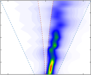
The upcoast event shown in figure 5 occurred on 5 September, 11:00, during a  ${\approx }5\,{\rm m}\,{\rm s}^{-1}$ upcoast wind and in the presence of an offshore short swell with peak period ${\approx }7$ s, significant height ${\approx }1.34$ m; (figure 5(a) and table). Mean currents at the near-shore array were less than $11\,{\rm cm}\,{\rm s}^{-1}$, flowing overall downcoast (figure 5a). The wavenumber–frequency spectra exhibit a combination, at different frequencies, of free and trapped power, the latter showing strong upcoast directional asymmetry.

Figure 5. Example of upcoast-propagating edge waves, matching the direction wind, with normally incident swells (observations on 5 September, 11:00). Notations and conventions are the same as in figure 3.
2.3. Preliminary conclusions
The events discussed above are examples of cases where the dominant propagation direction of the mostly trapped IG wave field is clearly correlated to wind direction, but seems disconnected from the direction of the swell (shore normal) and along-shore currents. We caution that this ‘associative’ logic might be misleading in general, because it assumes that the forcing (by either wind or waves) varies slowly and the IG wave system is at quasi-equilibrium. However, figures 4 and 5 represent only ‘1 h snapshots’ (processed time span) of the wave and wind fields. A directional misalignment might occur, for example, if the analysis window coincided with a major shift in swell direction, but before the IG wave field had time to respond. A quick examination of the details of the wind and wave fields before the events (figure 6), however, shows no significant shifts in the swell direction in the day before the selected events, which supports the suggestion that for these events wind, rather than swell, is the dominant forcing of the observed edge-wave wave field. Alternative interpretations of the reported asymmetry of edge-wave propagation are discussed in § 5.

3. Wind excitation of edge waves
3.1. Formulation of the problem
To our knowledge the possibility of wind generation of edge waves has never been examined theoretically. Here, we address this gap by considering mathematical models of direct edge-wave excitation by wind. To this end we adopt the idealizations outlined in the previous section: we assume the coastline to be straight and infinite, the bathymetry to be cylindrical, i.e. we allow the water depth to depend only on the distance from the straight shore. We employ the Cartesian coordinate frame with the horizontal  $y$ axis directed along the coastline, $x$ axis directed off shore and the vertical $z$ axis directed upwards. The edge waves are described in the shallow water approximation. We use the following notations: $u$ and $v$ are the offshore and the along-shore fluid velocity components, $H(x)$ is the undisturbed water depth, $p_a$ is total normal stress caused by the action of the atmosphere at the water surface and $\xi$ is the water surface elevation. Then the equations of motion can be written in the form
 \begin{gather} \frac{\partial u}{\partial t} + v\frac{\partial u}{\partial y} + u\frac{\partial v}{\partial x}+ g\frac{\partial \xi}{\partial x}={-}\frac{1}{\rho} \frac{\partial p_a}{\partial x}, \end{gather}
 \begin{gather} \frac{\partial v}{\partial t} + v\frac{\partial u}{\partial y} + u\frac{\partial v }{\partial x}+ g\frac{\partial \xi}{\partial y} ={-}\frac{1}{\rho} \frac{\partial p_a}{\partial y}, \end{gather}
 \begin{gather} \frac{\partial \xi}{\partial t}+\frac{\partial}{\partial y}v[\xi+H(x)]+\frac{\partial}{\partial x}u[\xi+H(x)]=0. \end{gather}
We confine our consideration to the linear setting. As shown by Longuet-Higgins (Reference Longuet-Higgins1969a), the effect of an oscillating shear stress at the water surface  $T_a$ in a viscous fluid in the presence of a propagating surface wave is equivalent to that of the normal stress with ${\rm \pi} /2$ phase lag relative to $T_a$. Here, $p_a$ in ((3.1) and (3.2)) is a sum of the direct normal stress at the water surface and the contribution of the shear stress. On linearizing system ((3.1)–(3.3)), we consider an infinitesimal plane wave propagating along the coastline
 \begin{gather} \frac{\partial u}{\partial t}+ g\frac{\partial \xi}{\partial x}={-}\frac{1}{\rho} \frac{\partial p_a}{\partial x}, \end{gather}
 \begin{gather} \frac{\partial v}{\partial t}+ g\frac{\partial \xi}{\partial y}={-}\frac{1}{\rho} \frac{\partial p_a}{\partial y}, \end{gather}
 \begin{gather} \frac{\partial \xi}{\partial t}+ H(x) \left(\frac{\partial u}{\partial x}+\frac{\partial v}{\partial y}\right)+u\frac{{\rm d}H}{{\rm d}\kern0.7pt x}=0. \end{gather}
We perform Fourier transform with respect to along-shore coordinate  $y$ and time $t$. For each harmonic component specified by a particular wavenumber $k$ the wave velocities, the elevation of the water surface and the normal stress can be presented as products of a function specifying the cross-shore dependence which we mark by a hat symbol and ${\rm e}^{-{\rm i}(\omega t - ky)}$
 \begin{equation} \left( \begin{array}{@{}ll} u \\ v \\ \xi \\ p_a \end{array} \right) = \left( \begin{array}{@{}ll} \hat U(x) \\ \hat V(x) \\ \hat \varXi(x) \\ \hat P_a (x) \end{array} \right) {\rm e}^{-{\rm i}(\omega t - ky)}. \end{equation}
Edge-wave cross-shore dependence is determined by the boundary value problem
 \begin{equation} gH(x)\left(\frac{{\rm d}^2 \hat\eta}{{{\rm d}\kern0.7pt x}^2}-k^2 \hat\eta\right)+ g \frac{{\rm d}H}{{\rm d}\kern0.7pt x} \frac{{\rm d} \hat \eta}{{\rm d}\kern0.7pt x} + \omega^2 \hat\eta = \frac{\omega^2 \hat P_a (x)}{\rho g}, \quad \hat\eta(0)< \infty, \quad \eta(\infty)=0, \end{equation}
where
 \begin{equation} \hat\eta(x) = \hat\varXi(x) + \frac{\hat P_a(x)}{\rho g}. \end{equation}
To fix the idea we consider the simplest model of bathymetry. For the constant slope,  $H(x)= \gamma x$, the explicit solution corresponding to the fundamental mode of edge waves is remarkably simple
 \begin{equation} \hat\eta (x) = a{\rm e}^{{-}kx},\quad \hat P_a (x) = P_{a0} {\rm e}^{{-}kx}, \quad \omega^2 - \gamma g k = \frac{\omega^2}{\rho ga} P_{a0}. \end{equation}
It differs from the similar formulae for free edge waves in Appendix A by the presence of the term  $({\omega ^2}/{\rho ga}) P_{a0}$ which accounts for the interaction with atmosphere. Since it is of the order of the air-to-water density ratio we can neglect its effect on the real part of the eigenvalue and present the wave frequency and the growth rate as follows:
 \begin{gather} \omega_0 = \sqrt{\gamma g k}, \end{gather}
 \begin{gather} \frac{\mathrm{Im} \omega}{\omega_0} = \frac{1}{2 \rho g} \mathrm{Im} \frac{P_{a0}}{a}. \end{gather}
 At first glance the above problem set-up strongly resembles the formulation for the Greenspan (Reference Greenspan1956) resonance, where an edge wave in resonance with a moving pressure distribution is generated by a moving, given, atmospheric pressure disturbance. The key difference with our set-up is that, in contrast to Greenspan (Reference Greenspan1956), there is no prescribed atmospheric pressure disturbance,  $P_{a0}$ is not given, but has to be found by solving the linear boundary value problem (3.8)–(3.12) in the absence of atmospheric forcing. Here, the challenge is to find and quantify instability mechanisms producing noticeable growth rates $\mathrm {Im}\, \omega > 0$. We identify three a priori seemingly plausible options which we examine:
(i) Edge-wave dispersion relation for any bathymetry allows the waves to have a critical layer in the wind flow. Therefore, the obvious candidate mechanism of edge-wave generation to be considered is an analogue of Miles’ mechanism of wind wave generation. This mechanism is examined in Appendix B for the main mode in the constant slope model; the growth rate is shown to be identically zero.
(ii) Since the edge waves are essentially quasi-horizontal motions, the shear stresses caused by the coupled atmospheric flow potentially might cause an instability if the turbulent viscosity in the boundary layer in the air is taken into account. This possibility is examined in Appendix C. It is shown that with viscous effects taken into account there is no instability in the system of edge waves coupled with atmospheric flow.
(iii) It is known (Longuet-Higgins Reference Longuet-Higgins1969b) that the effect of strongly wind-forced short free waves (of short gravity and gravity–capillary range) is equivalent to a viscous tangential stress at the surface. Since such short waves are strongly affected by orbital velocities of edge waves, these stresses are modulated by edge waves. Interaction of random free short waves with an edge-wave field might lead to self-excitation of a coherent edge wave. In the next section we examine such a ‘maser’ mechanism and show that, indeed, such self-excitation can occur. We will also provide rough estimates of its efficiency.
4. The ‘maser’ mechanism of self-excitation of edge waves
Since we have shown that, on the one hand, there is observational evidence of edge-wave excitation by wind, while, on the other hand, according to the analysis in Appendices B and C, there is no direct linear generation of edge waves by wind, at least in the simplest setting we outlined, there should be a less straightforward mechanism. In this section we re-examine the idea of the nonlinear ‘maser’ mechanism, suggested by Longuet-Higgins (Reference Longuet-Higgins1969b) in a different context and show that this is the most likely candidate for generation of edge waves by wind. Longuet-Higgins (Reference Longuet-Higgins1969b) showed that a harmonic short wave of gravity or gravity–capillary range with amplitude  $A$, wave vector $\boldsymbol {K}$ and frequency $\varOmega$ generates mean vorticity near the water surface, as if generated due to action of the viscous shear stress
 \begin{equation} \boldsymbol{\tau}_{wave} = 2 \rho \nu (KA)^2 \varOmega \frac{\boldsymbol{K}}{K}, \end{equation}
where  $\nu$ is the kinematic viscosity of the water. In our context, the short wind waves are always in the deep water regime and hence relation (4.1) applies. The presence of an edge wave, which is much longer than the short wave, causes modulation of its slope ( $KA$) and, hence, the modulation of the viscous shear stress given by (4.1). Obviously, the variations of the shear stress at the water surface have the same frequency and wavenumber as those of the edge wave. Crucially, these variations are phase linked with the edge wave, which therefore can cause growth of the edge wave. Note that, in our context, the maser mechanism is expected to be much more efficient than for deep water waves case examined by Longuet-Higgins (Reference Longuet-Higgins1969b), since the group velocities of short wind waves could be much closer to or even coincide with edge-wave celerity. Although in this case we do not have direct generation of edge waves by wind, here, we adopt the universally accepted terminology by Longuet-Higgins, who discovered this mechanism in a different context and christened it ‘maser mechanism of wave generation by wind.’ To estimate the growth rate of the edge wave we consider below two models of a surface wave field: (i) a toy model of the quasi-harmonic wave and, (ii) a reasonably realistic model with a continuous spectrum of random weakly nonlinear short wind waves. From now on, when we are speaking about a free surface wave field or short wind waves we mean only waves of short gravity and gravity–capillary range, since the rest of the surface wave spectrum plays no role in our consideration.
4.1. Edge-wave excitation by wind in the model with a quasi-harmonic wind wave
We start with examining the modulation of the amplitude and wavenumber of a short quasi-monochromatic wind wave by an edge wave. In the laboratory frame the local dispersion relation linking the short-wave frequency  $\varOmega$ with the wave vector $\boldsymbol K (K_x, K_y)$ riding upon the edge wave with the account of the Doppler shift due to the orbital velocity $\boldsymbol U (U, V)$ is
 \begin{equation} \varOmega = \sqrt{gK + \sigma K^3} + UK_x + VK_y, \quad K = \sqrt{K^2_x + K^2_y}, \end{equation}
where  $\sigma$ is the surface tension coefficient. In the reference frame following the edge wave with phase velocity $c$ this dispersion relation takes the form
 \begin{equation} \varOmega ={-}cK_y + \sqrt{gK + \sigma K^3} + UK_x + VK_y, \quad K = \sqrt{K^2_x + K^2_y}. \end{equation}
Recall that  $U$ and $V$ are the edge-wave orbital velocity components
 \begin{equation} (U,V)= \frac{gka}{\omega} {\rm e}^{{-}kx} (-\sin ky, \cos ky ). \end{equation}
The standard WKB (Wentzel–Kramers–Brillouin) equations for the wavevector  $\boldsymbol K (K_x, K_y)$ and position vector $\boldsymbol {r}$ of the short-wave wavepacket (e.g. Phillips Reference Phillips1977)
 \begin{equation} \frac{{\rm d} \boldsymbol{K}}{{\rm d}t} ={-} \frac{\partial \varOmega}{\partial \boldsymbol{r}}, \quad \frac{{\rm d} \boldsymbol{r}}{{\rm d}t} = \frac{\partial \varOmega}{\partial \boldsymbol{K}}, \end{equation}
in our context take the form
 \begin{equation} \left. \begin{gathered} \frac{{\rm d}K_x}{{\rm d}t}=({-}K_x \sin ky + K_y \cos ky ) \frac{gak^2}{\omega} {\rm e}^{{-}kx}, \quad \frac{{\rm d}K_y}{{\rm d}t}=(K_x \cos ky + K_y \sin ky ) \frac{gak^2}{\omega} {\rm e}^{{-}kx}, \\ \frac{{\rm d}y}{{\rm d}t}={-}c + \frac{gak}{\omega} {\rm e}^{{-}kx} \cos ky + C_{gry}, \quad \frac{{\rm d}\kern0.7pt x}{{\rm d}t}={-}\frac{gak}{\omega} {\rm e}^{{-}kx} \sin ky + C_{grx}. \end{gathered} \right\} \end{equation}
Here,
 \begin{equation} C_{gry} = \frac{K_y}{K}C_{gr},\quad C_{grx} = \frac{K_x}{K}C_{gr}, \quad \left(C_{gr} = \frac{{\rm d}}{{\rm d}K}\sqrt{gK + \sigma K^3}\right) \end{equation}
are the components of the intrinsic group velocity of the short wind waves. For simplicity only, consider a gravity–capillary wave, which initially has the wave vector directed along  $y$:
$y$:  $\boldsymbol {K}(t=0) = (0, K_0)$. Then, in the linear approximation in the amplitude of the edge wave ( $ka$), the solution to system (4.6) is
 \begin{gather} K_y = K_0 + K_0 \frac{gk^2 a}{\omega} \frac{\cos{ky}}{\omega - C_{gr0} k} {\rm e}^{{-}kx}, \end{gather}
 \begin{gather} K_x ={-}K_0 \frac{gk^2 a}{\omega} \frac{\sin ky}{\omega - C_{gr0} k} {\rm e}^{{-}kx}. \end{gather}
Here,  $C_{gr0}$ is the group velocity of a short wave with the initial wave vector $K_0$
$K_0$
 \begin{equation} C_{gr0} = \frac{g + 3 \sigma K^2_0}{2 \sqrt{gK_0 + \sigma K^3_0}}. \end{equation}
Modulation of the short-wave amplitude can be easily found from the conservation of the wave action  $N$
$N$
 \begin{equation} N = \frac{F}{\varOmega - (V - c)K_y - UK_x}, \end{equation}
where  $\varOmega$ is given by (4.3), and
 \begin{equation} F= \frac{(\varOmega - (V - c)K_y - UK_x)^2}{2K}|A|^2, \end{equation}
is the intrinsic energy of the short wave with amplitude  $|A|$. To the first order in $ka$ the Taylor expansion of (4.3) gives for the short-wave wave action
 \begin{equation} N = C_{f0} \left(1 +\varepsilon \frac{C_{gr0} - C_{f0} }{C_{f0}} \cos{ky} {\rm e}^{{-}kx} \right) |A|^2, \end{equation}
where
 \begin{equation} \varepsilon = \frac{gk^2 a}{\omega} \frac{1}{\omega - C_{gr0}k}, \end{equation}
and  $C_{f0}=\sqrt {{g}/{K_0}+\sigma K_0}$ is the intrinsic phase velocity of the short wave. In the linear approximation in $ka$, (4.14) and (4.8) yield the following closed expression for the slope of the short wave:
 \begin{equation} (KA)^2 = (K_0 A_0)^2 \left( 1 + \frac{3C_{f0} - C_{gr0}}{C_{f0}} \frac{gk^2 a}{\omega(\omega - C_{gr0}k)} \cos ky {\rm e}^{{-}kx} \right). \end{equation}
The shear stress due to the wind-forced short wave is given by (4.1). The wave frequency in the linear approximation can be found from (4.3). To the first order in  $ka$ we have
 \begin{equation} \varOmega = \varOmega_0 \left( 1 + \varepsilon \frac{C_{gr0}}{C_{f0}}\cos{ky}{\rm e}^{{-}kx}\right), \end{equation}
where  $\varOmega = \sqrt {gK + \sigma K^3}$ is the frequency of the gravity–capillary wave with wavenumber $(0,K_0)$. The effective shear stress created as a result of interaction with the edge wave reads
 \begin{equation} \boldsymbol{\tau}_{wave} = 2 \rho \nu (KA)^2 \varOmega = 2 \rho \nu (K_0 A_0)^2 \varOmega_0 \left( 1 + \frac{3 gk^2 a}{\omega(\omega - C_{gr0}k)} \cos ky {\rm e}^{{-}kx} \right) \boldsymbol{y_0}, \end{equation}
where  $\boldsymbol {y_0}$ is the unit vector in the $y$ direction. For the adopted simplest model with the constant slope bathymetry $H = \gamma x$ and the edge-wave dispersion relation $\omega = \sqrt {\gamma g k}$, we can now easily find the expression for the component of the shear stress acting upon the edge wave
 \begin{equation} \tau_{1y} = 6 \rho \nu (K_0 A_0)^2 \varOmega_0 \frac{gka}{\gamma (\omega - C^{(0)}_{gr}k)}. \end{equation}
Employing this expression for the shear stress we can finally obtain from (3.12) the normalized growth rate  $\omega _1/\omega _0$ of the edge wave of frequency $\omega _0, \,\omega _0 = \sqrt {\gamma g k}$
 \begin{equation} \frac{\omega_1 }{\omega_0} = \frac{3 \nu (K_0 A_0)^2 \varOmega_0 k^2}{\gamma \omega^2_0 (1 - C^{(0)}_{gr}k / \omega_0)}=\frac{3 \nu (K_0 A_0)^2 \varOmega_0 k}{\gamma^2 g (1 - C^{(0)}_{gr}k / \omega_0)} . \end{equation}
On the basis of this formula a rough estimate of the edge-wave relative growth rate  $(\omega _1 / \omega _0)$ for typical parameters ( $\nu = 10^{-6}\,\textrm {m}^2\,\textrm {s}^{-2}$, $\gamma \sim 10^{-3}-10^{-2}$, $k \sim 10^{-2}\,\textrm {m}^{-1}$, $C_{gr0} \sim 0.5\,\textrm {m}\,\textrm {s}^{-1},$ ) yields
 \begin{equation} \omega_1 / \omega_0 \sim 10^{{-}2} (K_0 A_0)^2. \end{equation}
Since typical short gravity and gravity–capillary waves are often rather steep (e.g. Troitskaya et al. (Reference Troitskaya, Sergeev, Kandaurov, Baidakov, Vdovin and Kazakov2012), where  $|A_0K_0 | \sim 0.23$), then $\omega _1 / \omega _0 \sim 10^{-3}$, which is quite substantial. However, the estimates strongly depend on the local conditions.
Obviously, the assumption of quasi-monochromatic short wind wave field adopted in the considered toy model is totally unrealistic, it was needed as a first step to fix the idea. The rough estimate it provides has a limited purpose, it suggests that edge-wave generation by wind via short wind waves is indeed feasible and, hence, a consideration of a more realistic model is warranted. Such a model is put forward in the next section.
4.2. Self-excitation of an edge wave interacting with a continuous spectrum of random short wind waves
Here, we consider a reasonably realistic model where short wind waves are described as an arbitrary continuous spectrum of nonlinearly interacting random weakly nonlinear waves, while the edge-wave field is assumed to be linear. The evolution of interacting random weakly nonlinear short gravity and gravity–capillary waves is described using the kinetic equation for the spectral density of wave action  $N$ (e.g. Keller & Wright Reference Keller and Wright1975)
 \begin{equation} \frac{\partial N}{\partial t} + \frac{\partial \varOmega}{\partial \boldsymbol{K}} \frac{\partial N}{\partial \boldsymbol{r}} - \frac{\partial \varOmega}{\partial \boldsymbol{r}} \frac{\partial N} {\partial \boldsymbol{K}} = \beta[U,V]N + Int[N], \end{equation}
where the term  $\beta N$ comprises energy input due to the interaction with wind and sinks due to dissipation, $\varOmega$ is the short-wave frequency specified by the dispersion relation (4.3), $\boldsymbol {K}$ is the short-wave vector and $Int[N]$ is the short-wave nonlinear interaction term. The full collision integral $Int[N]$, which for this range of scales has not been rigorously derived yet for the situations where both the triad and quartic interactions are important. The collision integral for the gravity range derived by Hasselmann (Reference Hasselmann1962) (e.g. Komen et al. Reference Komen, Cavaleri, Donelan, Hasselmann, Hasselmann and Janssen1994) is expected to be valid when the main effect is due to the waves of gravity range. There exist a number of parameterizations of the collision integral for the gravity–capillary range (see e.g. Kosnik, Dulov & Kudryavtsev Reference Kosnik, Dulov and Kudryavtsev2010, and reference therein). Here, instead of considering the full collision integral $Int[N]$, which for this range of scales remains to be properly derived, the nonlinear interaction of short gravity and gravity–capillary waves will be described by the simplest relaxation model commonly referred to as the $\tau$-approximation (e.g. Keller & Wright Reference Keller and Wright1975). This relaxation model is a commonly used approximation of the nonlinear interaction term based on the assumption that the spectrum of short waves differs little from the equilibrium spatially uniform spectrum $N_0(\boldsymbol {K})$ and is only slightly perturbed by the edge wave. The equilibrium spectrum $N_0(\boldsymbol {K})$ is determined by the balance between the input and relaxation specified by the right-hand side of the kinetic equation, i.e.
 \begin{equation} \beta[U, V]N^{(0)} + Int[N^{(0)}] = 0. \end{equation}
Consider a small spatially homogeneous perturbation  $N_1(\boldsymbol {K})$ of the equilibrium spectrum $N = N^{(0)} + N^{(1)}$. In virtue of our assumption $N^{(1)} \ll N^{(0)}$, the kinetic equation can be linearized, which yields
 \begin{equation} \frac{\partial N^{(1)}}{\partial t} = \frac{\delta}{\delta N^{(0)}}\beta[N^{(0)}]N^{(1)}N^{(0)} + \beta[N^{(0)}]N^{(1)} + \frac{\delta}{\delta N^{(0)}}Int[N^{(0)}]N^{(1)}. \end{equation}
This equation predicts that all perturbations are decaying exponentially
 \begin{equation} N^{(1)} = N^{(1)}_0 (K) \exp (-\beta_r (K)t), \end{equation}
where  $\beta _r (\boldsymbol {K})$ is the relaxation rate for the wave component with the wavevector $\boldsymbol {K}$. The inverse of $\beta _r (\boldsymbol {K})$ is the relaxation time $\tau$ which gave the name to this approach that originated in the kinetics of gases (Bhatnagar, Gross & Krook Reference Bhatnagar, Gross and Krook1954). The substitution of the spatially homogeneous solution (4.24) into (4.23) yields
 \begin{equation} -\beta_r N^{(1)}_0 = \left[ \frac{\delta}{\delta N^{(0)}}\beta[N^{(0)}]N^{(0)} + \beta[N^{(0)}] + \frac{\delta}{\delta N^{(0)}} Int [N^{(0)}] \right] N^{(1)}, \end{equation}
which means that the decay rate  $\beta _r$ is the eigenvalue of the operator in square brackets. Equation (4.25) yields the approximation of the perturbed ‘collision integral’ we employ
 \begin{equation} \frac{\delta}{\delta N^{(0)}} Int [N^{(0)}] N^{(1)} = \left[ - \frac{\delta}{\delta N^{(0)}}\beta[N^{(0)}]N^{(0)} - \beta[N^{(0)}] - \beta_r \right] N^{(1)}, \end{equation}
which, strictly speaking, can be justified only for the spatially homogeneous perturbation. Following Keller & Wright (Reference Keller and Wright1975), we will use this expression for small,  $N^{(1)},\,(N^{(1)}/ N^{(0)}\ll 1)$, weakly inhomogeneous perturbations of scales far exceeding those of gravity–capillary waves. Following Keller & Wright (Reference Keller and Wright1975), we also assume that $\beta _r$ is equal to the short-wave wind input $\beta _{wind} N^{(0)}$. Then, the kinetic equation for the perturbations of the wave action spectral density in the presence of edge waves takes the form
 \begin{equation} \frac{\partial N^{(1)} }{\partial t} + \frac{\partial \varOmega^{(0)}}{\partial \boldsymbol{K}} \frac{\partial N^{(0)}} {\partial \boldsymbol{r}} - \frac{\partial \varOmega^{(0)}}{\partial \boldsymbol{r}} \frac{\partial N^{(0)}} {\partial \boldsymbol{K}} ={-}\beta_{wind} (N^{(0)}) N^{(1)} , \end{equation}
were  $\varOmega ^{0} = \sqrt {gK + \sigma K^3}$ is the unperturbed frequency of the gravity–capillary wave with wave vector $\boldsymbol {K}$. It is more convenient to use the polar form for $\boldsymbol {K}=(K\sin \theta, K\cos \theta$ characterized by its modulus ${K}$ and polar angle $\theta$. Making use of the dispersion relation (4.3), we re-write our kinetic equation (4.27) in the form
 $$\begin{gather} \frac{\partial N^{(1)} }{\partial t} + \frac{C^{(0)}_{gr}}{K}(\boldsymbol{K} \boldsymbol{\nabla}) N^{(1)} - \frac{1}{K} \frac{\partial N^{(0)} }{\partial K} \left( K_y \frac{\partial (\boldsymbol{U}\boldsymbol{K})}{\partial y} + K_x \frac{\partial (\boldsymbol{U}\boldsymbol{\cdot}\boldsymbol{K})}{\partial x} \right) \nonumber\\ - \frac{1}{K^2} \frac{\partial N^{(0)} }{\partial \theta} \left( - K_x \frac{\partial (\boldsymbol{U}\boldsymbol{\cdot}\boldsymbol{K})}{\partial y} + K_y \frac{\partial (\boldsymbol{U}\boldsymbol{\cdot}\boldsymbol{K})}{\partial x} \right) ={-} \beta_{wind} (N^{(0)}) N^{(1)}, \end{gather}$$
where,
 \begin{equation} \boldsymbol{U}=(U,V), \quad \boldsymbol{U}=\boldsymbol{U_0}\exp({-{\rm i}(\omega t - ky) -kx}), \end{equation} $C^{(0)}_{gr}= \textrm {d} \varOmega ^{(0)} / \textrm {d}K$ and $\beta _{wind}N^{(0)}$ is the input minus dissipation in the absence of edge waves. Since the problem is linear with respect to the edge-wave amplitude, it is convenient to present the fields in complex form. Then, taking into account (4.3)
 \begin{equation} \boldsymbol{U_0} = \frac{gka}{\omega} (i, 1). \end{equation}
We consider the perturbations of wave action spectral density  $N^{(1)}$ in the form of a harmonic inhomogeneous wave repeating the structure of the orbital velocity field in the edge wave
 \begin{equation} N^{(1)} = N^{(1)}_0 \exp({-{\rm i}(\omega t - ky)-kx}). \end{equation}
Then, from the kinetic equation (4.27) we obtain the following expression for the perturbation amplitude  $N^{(1)}_0$:
 \begin{equation} N^{(1)}_0 ={-} \frac{gk^2 a}{\omega^2} \frac{(K_y+{\rm i}K_x)^2}{(1- C^{(0)}_{gr}(k / \omega) (K_y + {\rm i}K_x) / K + \beta {\rm i} / \omega)} \frac{1}{K} \left(\frac{\partial N^{(0)}}{\partial K} + {\rm i} \frac{1}{K} \frac{\partial N^{(0)}}{\partial \theta} \right). \end{equation}
Since  $K_y = K \cos \theta$, $K_x = K \sin \theta$, we can present the above expression (4.32) in a more compact form
 \begin{equation} N^{(1)}_0 ={-} \frac{gk^2 a}{\omega^2} \frac{K^2 {\rm e}^{2{\rm i} \theta} }{(1- C^{(0)}_{gr}(k / \omega) {\rm e}^{{\rm i} \theta} + \beta {\rm i} / \omega)} \frac{1}{K} \left(\frac{\partial N^{(0)}}{\partial K} + {\rm i} \frac{1}{K} \frac{\partial N^{(0)}}{\partial \theta} \right). \end{equation}
Taking into account the relationship between the wave action spectral density  $N$, the spectrum of surface elevations $F$ (
$F$ ( $N=F/ \varOmega$) and the slope spectra $S=FK^2$ (4.33), we can readily obtain an expression for the perturbation of the slope spectra $S^{(1)}$ caused by the edge wave
 \begin{equation} S^{(0)} = S^{(1)}_0 \exp({-{\rm i}(\omega t - ky)-kx} ). \end{equation}
Then, the complex amplitude  $S^{(1)}_0$ is
 \begin{equation} S^{(1)}_0 ={-} \frac{gk^2 a}{\omega^2} \frac{\omega K {\rm e}^{2{\rm i} \theta} } {(\omega - k C^{(0)}_{gr}{\rm e}^{{\rm i} \theta} + \beta {\rm i} )} \left(\frac{\partial S^{(0)}}{\partial K} - \frac{S^{(0)}}{K} \left( \frac{C^{(0)}_{gr}}{C^{(0)}_{ph}} + 2 \right) + {\rm i} \frac{1}{K} \frac{\partial S^{(0)}}{\partial \theta} \right), \end{equation}
and  $C^{(0)}_{ph} = {\varOmega ^{(0)} }/{K}$. We can now calculate the spectral density of the perturbed tangential stress $\boldsymbol {\tau }^{(1)}$
 \begin{equation} \boldsymbol{\tau}^{(1)} (\boldsymbol{K}) = \boldsymbol{\tau}^{(1)}_0 (\boldsymbol{K}) \exp({-{\rm i}(\omega t \!-\! ky)-kx}),\quad \left( \boldsymbol{\tau}^{(1)}_0 (\boldsymbol{K}) = 2\rho \nu S^{(1)}_0 \varOmega (\boldsymbol{y}_0 \cos \theta \!+\! \boldsymbol{x}_0 \sin \theta)\right), \end{equation}
where  $\boldsymbol {y}_0$ and $\boldsymbol {x}_0$ are unit vectors in the along-shore and offshore directions. The integration of (4.36a,b) over the short-wave wavevectors yields the surface shear stress caused by the short-wave spectrum
 \begin{equation} \boldsymbol{\tau}_{10}= 2\rho \nu \int S^{(1)}_0 (\boldsymbol{y}_0 \cos \theta + \boldsymbol{x}_0 \sin \theta) \sqrt{gK +\sigma K^3} K\,{\rm d}K\,{\rm d} \theta. \end{equation}
For rough estimates we assume that the equilibrium short-wave spectrum is the saturated Phillips spectrum (Phillips 1958)
 \begin{equation} S^{(0)} = \frac{\alpha \cos (\theta - \theta_0)^2}{K^2}, \end{equation}
where  $\theta _0$ is the wind direction with respect to the $y$ axis which can vary from $-{\rm \pi} / 2$ to ${\rm \pi} / 2$, while the Phillips constant $\alpha = 0.02$. Then, making use of the dispersion relation for edge waves, we find from (4.35) the complex amplitude of the perturbation of the short-wave field slopes in the form
 \begin{equation} S^{(1)}_0 = \frac{k a \omega}{\gamma} {\rm e}^{2{\rm i} \theta} \dfrac{\left( \left( 4 - \dfrac{C^{(0)}_{gr}}{C^{(0)}_{ph}} \right) \cos (\theta - \theta_0)^2 -{\rm i} \sin 2(\theta - \theta_0)\right) }{(\omega - k C^{(0)}_{gr} {\rm e}^{{\rm i} \theta}) + \beta {\rm i} } \frac{\alpha}{K^2}. \end{equation}
From the definition of tangential stress (4.36a,b) it follows
 \begin{gather} \boldsymbol{\tau}^{(1)}_{0} = \frac{2 \rho \nu \omega \alpha}{\gamma} ka \boldsymbol{\cdot} \end{gather}
 \begin{gather} \int^{K_{max}}_{K_{min}}\frac{{\rm d}K}{K} \int^{{\rm \pi} / 2}_{- {\rm \pi}/ 2} {\rm e}^{2{\rm i} \theta} \frac{ \left( 4 - \dfrac{C^{(0)}_{gr}}{C^{(0)}_{ph}} \right)\cos (\theta - \theta_0)^2 - {\rm i} \sin 2(\theta - \theta_0) }{(\omega - k C^{(0)}_{gr} {\rm e}^{{\rm i} \theta}) + \beta {\rm i} }\nonumber\\ (\boldsymbol{y}_0 \cos \theta + \boldsymbol{x}_0 \sin \theta) \sqrt{gK +\sigma K^3} \,{\rm d} \theta. \end{gather}
Since the spatial distribution of short-wave packets riding on edge waves is modulated by the edge waves, this creates the tangential stress which is phase linked to the edge wave and, thus, might lead to selection and self-excitation of the selected edge wave. The growth rate of the edge wave can be calculated employing (3.12), which yields
 $$\begin{gather} \frac{\mathrm{Im} \omega}{ \omega} =\frac{\nu \omega \alpha k}{ g \gamma^2 } \mathrm{Re} \int^{K_{max}}_{K_{min}} \frac{{\rm d}K}{K} \int^{{\rm \pi} / 2}_{- {\rm \pi}/ 2} {\rm e}^{3{\rm i} \theta} \frac{\left[ \left( 4 - \dfrac{C^{(0)}_{gr}}{C^{(0)}_{ph}} \right) \cos (\theta - \theta_0)^2 -{\rm i} \sin 2(\theta - \theta_0)\right] }{(\omega - k C^{(0)}_{gr} {\rm e}^{{\rm i} \theta}) + \beta {\rm i} }\nonumber\\ \times \sqrt{gK +\sigma K^3} \,{\rm d}\theta. \end{gather}$$
For the estimates we use the values of parameters from Sheremet et al. (Reference Sheremet, Guza, Elgar and Herbers2002) ( $\omega = 0.088 c^{-1}$, $\gamma = 0.02$, $k = 0.037 m^{-1}$). If, for simplicity, we also assume that $\omega / k \gg C^{(0)}_{gr}$, although this assumption significantly underestimates the effect and is often not justified, then expression (4.42) takes a much simpler form
 \begin{equation} \frac{\mathrm{Im} \omega}{ \omega} = \frac{\nu \alpha k}{ \sqrt{g} \gamma^2 } \mathrm{Re} \left[ \int^{{\rm \pi} / 2}_{- {\rm \pi}/ 2} {\rm e}^{3{\rm i} \theta} \left( \frac{7}{2} \cos (\theta - \theta_0)^2 -{\rm i} \sin(\theta - \theta_0) \right) \,{\rm d} \theta \int^{K_{max}}_{K_{min}} \frac{{\rm d}K}{\sqrt{K}} \right]. \end{equation}
The integral with respect to  $K$ in (4.43) logarithmically diverges at the upper and lower limits. Obviously, there is a viscous ‘cutoff scale’ specified by viscosity which is not explicitly taken into account in the presented model. Therefore, for our rough estimates we introduce the ‘cutoff scale’ $K=10^2\,\textrm {m}^{-1}$ as the upper limit of integration. Then, according to (4.43), for the above parameters and viscosity coefficient equal to the kinematic viscosity of water $\nu = 10^{-6} \,\textrm {m}^2\,\textrm {s}^{-1}$, $\mathrm {Im}\, \omega / \omega \sim 10^{-5}$. However, since a background small-scale turbulence is always present in the upper layer of the ocean, the use of turbulent viscosity is more appropriate. We estimate the eddy viscosity coefficient by the Prandtl formula $\nu = 0.4 w_* z$, where $w_*$ is the friction velocity in the water boundary layer linked to the air friction velocity by the condition of the equality of shear stresses $\rho _{air} u^2_* = \rho _{water} w^2_*$. We assume that the eddy viscosity for a wave with the wavenumber $K$ is $\nu = 0.4 w_* K^{-1}$. Then, from (4.43) follows
 \begin{equation} \frac{\mathrm{Im} \omega}{ \omega} = \frac{0.4 u_* \alpha k}{ \sqrt{g} \gamma^2 } \sqrt{\frac{\rho_a}{\rho_w}} \mathrm{Re} \left[ \int^{{\rm \pi} / 2}_{- {\rm \pi}/ 2} {\rm e}^{3{\rm i} \theta} \left( \frac{7}{2} \cos (\theta \!-\! \theta_0)^2 - {\rm i} \sin(\theta \!-\! \theta_0) \right) \,{\rm d} \theta \int^{K_{max}}_{K_{min}} \frac{{\rm d}K}{K^{3/2}} \right]. \end{equation}
The integral with respect to  $K$ in (4.44) also diverges at the lower limit as $K_{min}\rightarrow 0$. The simplifications adopted in the model break down for insufficiently short wind waves. Longer short wind waves have larger group velocities and therefore are increasingly less sensitive to inhomogeneities created by the orbital velocities of edge waves. In our estimates we set the large-scale ‘cutoff’ to be equal to $4\,\textrm {m}^{-1}$, which corresponds to the wavelength of 1.5 m. For the friction velocity corresponding to a 10–12 $\textrm {m}\,\textrm {s}^{-1}$ wind and the above mentioned parameters of the edge wave from (4.44), expression (4.44) predicts quite substantial growth rates: $\mathrm {Im} \omega / \omega \sim 10^{-3}-10^{-2}$.
These estimates are quite crude and, therefore, the specific quantitative predictions should be treated very cautiously; a healthy scepticism would be appropriate. However, we could deduce from the formulae ((4.42) and (4.44)) the most basic qualitative features which we expect to be robust. Neither the specificity of the adopted bathymetry nor the choice of the main mode are important here. What matters most is the characteristic phase velocity of edge waves controlled in our simplest model by the bottom slope  $\gamma$. For real bottom topographies the same role will be played by a ‘characteristic bottom slope.’ We expect the inverse quadratic dependence of the growth rates on characteristic bottom slope to be the most robust feature of this mechanism of edge-wave generation. Roughly, the milder the beach slope the more favourable are the conditions for the generation of an edge wave by wind. This prediction goes with a caveat; the bottom friction was ignored in the model and this oversimplification might preclude the generation of edge waves for particularly small bottom slopes. In its present form the model does not yield explicitly the distinguished preferred scale of edge waves. All things being equal, the excitation is expected to be stronger for shorter edge waves. The preferred scale of edge-wave excitation could be found by simulating directly equation (4.42) without extra simplifications, which goes beyond the scope of this paper and requires a dedicated work.
Implicit in the model is the key assumption of moderate wind. For winds too weak the steepness of gravity–capillary waves will be too small and since the mechanism is quadratic in steepness, their effect on edge waves will be negligible. On the other hand, for winds too strong the short waves might be breaking intensively and will be less sensitive to the inhomogeneity due to orbital velocities of the edge wave; the scale of inhomogeneity should be always smaller than the mixing scale due to wind. To quantify what winds are moderate enough and what are not, is a challenging task which goes beyond the scopes of the present work.
At present, there is a substantial gap between the maser model and observations. To bridge it concerted efforts from both ends of the divide are needed. From the observations we need detailed measurements of short wind waves, especially to determine whether there are phase correlations with the edge waves; difficult to provide accurate measurements of subsurface turbulence are necessary to find the scale-dependent turbulent viscosity for short wind waves. On the theoretical side the most crude approximation should be replaced by more accurate alternatives, of particular concern is the use of the long-wave cutoff. To this end, better models of short-wave interaction with the turbulent boundary layer are required. A novel kinetic equation which takes into account both the triad and quartet interactions should be derived and investigated numerically.
5. Concluding remarks
Here, we briefly summarize the main results: a plausible theoretical model of edge-wave excitation by wind and an analysis of the data set from the SandyDuck’97 near-shore field experiment strongly suggest the occurrence of edge waves generated by wind. We also discuss some implications of the results and the new questions this work raises.
Our analysis in § 2 of the data set from the SandyDuck’97 near-shore field experiment has shown the occurrence of pronounced directional asymmetry of edge waves unrelated to the direction of swells and along-shore currents. We interpret this as a strong suggestion of direct generation of edge waves by wind. We see two possible alternative interpretations of the observed directional asymmetry. First, the observed edge waves have not necessarily be generated locally, these edge waves might have been generated by swell at a different stretch of the coast oriented obliquely with respect to the incoming swell. Such edge waves, in principle, could propagate long distances along shore. We also note that that a related interpretation of the observed edge-wave directional asymmetry as an artefact of non-local in time generation by swell, i.e. generation by oblique swell coming onshore well before the moment of observation, was not supported by the SandyDuck’97 data. The second alterative is due to the possibility that incoming swell might consist of several swell systems and smaller peaks in the spectra, which we do not see in the observations because of wave–buoy system limitations, might still generate edge waves via resonant interactions; the poor angular resolution of the SandyDuck’97 swell spectra does not enable us to rule out this possibility. However, we stress that these two mechanisms do not contain inherent directional asymmetry, a priori edge waves could come from both directions with equal probability. We do not see signs of this in our data set, and with the caveats that our data set is limited, we could cautiously claim that the data do not support these alternative interpretations.
The analysis of the SandyDuck’97 data set also highlighted the fundamental limitations of the available data sets and techniques. The main limitation is the overwhelming challenge posed by deploying and maintaining spatial arrays of sensors with high-enough sensor density and large-enough along-shore spans to resolve the distribution of power in the along-shore lag space. As discussed in § 2, even the best existing data sets, which we do not expect to see matched in quality soon, have intrinsically low lag resolution and span. Because of this, all analysis techniques can return reliably only low-order moments of the spectral power distribution in the frequency–lag space; basically, only the location of the mean. While not useful for resolving individual edge-wave modes, fortunately, this is enough to identify the presence/absence of pronounced directional asymmetry. In this sense, the resulting conclusions on edge-wave directional asymmetry are robust. To obtain a better resolved picture of directional properties of edge waves qualitatively, new methods of edge-wave observation based on remote sensing are needed.
In the theoretical analysis we exploit the observation that edge waves are much slower than the free oceanic IG waves, more specifically, that the phase velocities of edge waves could be close to the group velocities of wind-forced short gravity and gravity–capillary waves. This makes likely effective edge-wave generation by wind through the self-excitation ‘maser’ mechanism: the wind-forced random short gravity and gravity–capillary waves modulated by edge-wave orbital velocities create non-uniform tangential stresses phase linked with the edge wave. Thus, similar to maser, out of the random field of linear edge waves one coherent harmonic edge wave is selected and amplified. This mechanism is expected to work most effectively when the celerity of edge waves falls into the range of group velocities of gravity–capillary or short gravity waves, which is often the case. Figure 7 illustrates the domain of overlap for the first few edge-wave modes on a plane beach with slopes ranging from 0.003 to 0.01. Most likely to be excited by the ‘maser’ mechanism are modes 0 and 1, but higher modes might also be excited on beaches with small enough slopes. Note that a proper consideration of small slopes requires taking into account bottom friction, and our model is frictionless. Also, in a realistic model one has to take into account both the along-shore current and wind-induced Ekman current which might significantly affect the dispersion relations of gravity–capillary waves. We describe the ‘maser’ excitation employing a model based on the kinetic equation for weakly nonlinear short gravity and gravity–capillary waves. This is the robust part of what we are putting forward. However, even knowing that for a given bathymetry the kinematic condition for interaction is satisfied and having an adequate mathematical model, we cannot say a priori without solving the kinetic equation whether the interaction is strong enough to be of importance. To solve the kinetic equation for waves on a current with periodic inhomogeneity (either numerically or analytically) is a quite challenging task. To circumvent somehow this formidable obstacle and to obtain a rough semi-quantitative estimate we adopted a number of simplifying assumptions. The key ones are the use of the ‘ $\tau$-approximation’ and introduction of a ‘cutoff’ scale in dealing with the divergence of the nonlinear term. The ‘ $\tau$-approximation’ assumes that the spectrum of short gravity and gravity–capillary waves is a sum of a steady longitudinally uniform equilibrium spectral distribution in the absence of perturbing edge waves and small time-dependent deviations from the equilibrium due to edge waves. The ‘ $\tau$-approximation’ originated as the model for collision processes in gases (Bhatnagar et al. Reference Bhatnagar, Gross and Krook1954) and is widely used beyond the parameter range of its theoretical validity in many physical contexts, including physical oceanography (e.g. Keller & Wright Reference Keller and Wright1975; Hughes Reference Hughes1978). The key element in the model is the fact that wind-forced short gravity and gravity–capillary waves exert a shear stress on the surface. This stress depends on the eddy viscosity near the surface, which can vary up to several orders of magnitude depending on the sea state (e.g. Huang Reference Huang1979). This introduces a large element of uncertainty into the estimates. We also have only a very rough idea on the long-wave boundary of the range of short gravity waves for which the adopted parametrization of the shear stress remains valid; in the sketch in figure 7 we used 1 m wavelength for certainty. By employing these approximations and assumptions we obtain a rough estimate for the growth rate of edge waves, which suggests that, indeed, the mechanism is effective under favourable conditions. However, at present, we cannot provide a more solid quantitative prediction, instead, here, we discuss open questions and some qualitative implications of this mechanism.

Figure 7. Group velocity of short gravity and gravity–capillary waves (black line, using the ASTM saltwater model with salinity of  $20\,\textrm {g}\,\textrm {kg}^{-1}$ and surface tension $0.076\,\textrm {N}\,\textrm {m}^{-1}$) and the phase velocity of the first few edge-wave modes on a plane beach with slopes of 0.003, 0.06 and 0.01. The left bound of the sketched edge waves corresponds to waves with 50 s period. The domain of velocity overlap is marked in grey.
An important implicit assumption we adopted is that the random edge waves are linear and, hence, not interacting with each other. Nonlinear interactions among edge waves, if sufficiently strong, can weaken or even destroy the coherent self-excitation. This issue goes beyond the scope of this work and requires a dedicated study. The coherent self-excitation mechanism is expected to be most favoured by moderate winds, since sufficiently strong winds reduce the spatial inhomogeneity of short gravity and gravity–capillary spectra caused by edge waves. However, at the moment we are unable to quantify the ‘optimal’ wind. To summarize, the overall weak point of the theoretical picture we put forward is that, currently, there are still many uncertainties requiring substantial further work to elaborate quantitatively their implications. At the qualitative level, under favourable conditions we expect literally visible manifestations of the maser mechanism for edge waves: orbital velocities of edge waves create inhomogeneities of the gravity–capillary wave field which can be visible to the unaided eye and/or microwave radars as roughness bands moving along shore with the celerity of edge wave. Similar manifestations of roughness bands moving onshore are commonly observed for internal gravity waves (e.g. Apel et al. Reference Apel, Byrne, Proni and Charnell1975), but we are not aware of such observations for edge waves. If confirmed, this way of observing edge waves might be an important addition to the existing toolbox.
We stress that we view the generation of edge waves by swell through triad interactions as the dominant mechanism of their generation. In the SandyDuck’97 data set, out of  ${\sim }$900 3 h runs exhibiting edge-wave events, we found only $\sim$70 that suggest possible wind generation. We focussed upon those relatively rare situations where edge-wave generation through triad interactions was either absent or weak, which made generation of edge waves by wind the most likely explanation of the observed directional asymmetry.
Although we showed that the ‘maser’ mechanism of edge-wave excitation is very plausible, this does not rule out other possibilities such as, for example, triad interactions between two edge-wave harmonics and a resonant perturbation in the airflow (Tsimring Reference Tsimring1983; Vrećica, Soffer & Toledo Reference Vrećica, Soffer and Toledo2019). In contrast to Vrećica et al. (Reference Vrećica, Soffer and Toledo2019) no specific information is readily available about possible atmospheric anomalies such as strong fronts during the Sandyduck97 experiment. Certainly, these possibilities need further investigation.
Albeit that the growth rates due to Miles’ mechanism and the viscous shear stresses created by wind are shown to vanish for the adopted constant slope model, for more general bathymetry the question remains open and needs further study.
Our main conclusion is that the question of wind contribution to edge-wave generation is open, it needs further investigation and in the generic situations both the nonlinear triad interactions and generation by wind should be simultaneously taken into account.
Funding
The work would not have happened without the support of NSFGEO-NERC via grants NSF no. 1737274 and NERC NE/R012202. Y.T. and I.S. acknowledge support within the framework of the State Assignment to the Institute of Applied Physics of the Russian Academy of Sciences (project no. 00350-2021-0007). The additional support by the Ministry of Education and Science of the Russian Federation (Task No. 0030-2021-0007) and by the Research and Education Mathematical Center ‘Mathematics for Future Technologies’ is also gratefully acknowledged by Y.T. and I.S.
Declaration of interests
The authors report no conflict of interest.
Appendix A. Spectral analysis in the wavenumber–frequency domain
Idealizing the FRF bathymetry as along-shore uniform, i.e.  $H=H(x)$ in the FRF coordinate system, where $H$ is the water depth, $x$ is the cross-shore coordinate, increasing seaward, and $y$ is the along-shore coordinate, linear edge waves may be described using the potential shallow water equations
 \begin{equation} \eta_{t}+\left(H\phi_{x}\right)_{x}+H\phi_{yy}=0;\quad\phi_{t}+g\eta=0, \end{equation}
where  $\eta (x,y,t)$ and $\phi (x,y,t)$ are the free surface elevation and the flow potential, and subscripts denote partial derivatives. Substituting a Fourier representation, e.g.
 \begin{equation} \eta(x,y,t)=\int_{-\infty}^{\infty}F(x,k) {\rm e}^{{\rm i}\left(ky-\omega t\right)}\frac{{\rm d}\kappa}{2{\rm \pi}}, \end{equation}
we obtain for the cross-shore function  $F$ the differential equation
 \begin{equation} \left(c^{2}F_{x}\right)_{x}+\left(\omega^{2}-c^{2}k^{2}\right)F=0, \end{equation}
where  $k$ is the along-shore wavenumber, $\omega =2{\rm \pi} f$ is the angular frequency and $c(x)=\sqrt {gH}$. The cross-shore structures $F$ corresponding to edge waves are solutions of (A3) that satisfy the boundary conditions
 \begin{equation} F(0)<\infty,\quad\text{and}\quad F(\infty)=0. \end{equation}
The boundary value problem (A3)–(A4a,b) is a singular SL eigenvalue problem, with  $F(x,k)$ being the eigenfunction corresponding to eigenvalue $\omega (k)$. Under quite general conditions, for a given $k$, the problem (A3)–(A4a,b) has a countable set of eigenvalues $\{ \omega _{n}\}$ with $n=0,1,\ldots$ (e.g. Huthnance Reference Huthnance1975). In the $(k,\omega )$ parameter space, edge-wave modes are represented by dispersion curves $\omega (k)$. For example, for a plane beach of constant slope $s$, the dispersion relation is $\omega ^{2}=gs(2n+1)k$ (e.g. Whitham Reference Whitham1979).
Standard edge-wave analysis in the  $(k,\omega )$ plane involves: (i) solving the SL problem (A3)–(A4a,b) for the bathymetry under consideration (FRF bathymetry in this case); and (ii) estimating the power density in $(k,\omega )$ plane. If spectral estimators had infinite resolution, overlapping power density and dispersion curves could be used to identify existing edge-wave modes. Although solving numerically the system of (A3)–(A4a,b) is not difficult (e.g. Holman & Bowen Reference Holman and Bowen1979; Kirby, Dalrymple & Liu Reference Kirby, Dalrymple and Liu1981; Howd et al. Reference Howd, Bowen and Holman1992), the low resolution of the observations (and, consequently, of the spectral estimates in the $(k,\omega )$ space) precludes accurate identification of individual edge-wave modes (see discussion below). It is, however, possible to answer a weaker question: ‘Are edge waves observed at all?’ Indeed, for a given frequency $\omega$, edge-wave wavenumbers identifiable by an along-shore line of instruments satisfy the constraint $k_{min}< k< k_{max}$. The lower bound is determined by the trapping condition $k>k_{min}^{E}={\omega ^{2}}/{g}$, where ${\omega ^{2}}/{g}$ is the deep water wavenumber. The upper bound is determined by the condition that the turning point of the trapped wave has to be seaward of the instrument line; setting to zero the coefficient of $F$ in (A3) determines the turning-point depth for modes with wavenumber $k$ as $H_{T}=({1}/{g})({\omega }/{k})$. A line of instruments located at an isobath $h_{0}$ can therefore only resolve wavenumbers $k< k_{max}^{E}=\sqrt {\omega /gH}$. In addition, on setting, according to convention $\omega \geq 0$, the sign of $k$ specifies the direction of propagation: upcoast for $k>0$ and downcoast for $k<0$. One can therefore identify edge-wave fields and evaluate their directional symmetry by the location of the power density peaks with respect to the interval $\pm [k_{min}^{E},k_{max}^{E}]$.
Estimates of wavenumber–frequency power density are based on along-shore lines of the near-shore array (figure 1b), following Davis & Regier (e.g. Reference Davis and Regier1977). Pressure frequency cross-spectra are estimated using the standard method (Welch Reference Welch1967): 3 h long time series are detrended, divided into 600 s de-meaned segments with 50 % overlap, tapered using a Hanning window, Fourier transformed and averaged over the 600 s segments. The resulting estimates have 34 degrees of freedom, a frequency resolution of 0.008 Hz and 26 frequency modes in the IG band ( $f\leq 0.05$ Hz).
The spatial lag structure of the cross-spectra at a given frequency are then used to estimate the spectral density in the wavenumber domain. Estimators of various complexity may be applied, such as the Maximum likelihood method (e.g. Capon Reference Capon1969; Pawka Reference Pawka1982; Oltman-Shay & Guza Reference Oltman-Shay and Guza1987; Donelan et al. Reference Donelan, Babanin, Sanina and Chalikov2015, and many others), maximum entropy method (MEM), (Lygre & Krogstad Reference Lygre and Krogstad1986; Wu Reference Wu1997; Sheremet et al. Reference Sheremet, Guza and Herbers2005, e.g.) or other similar ‘best-fit’ methods (Herbers et al. Reference Herbers, Orzech, Elgar and Guza2003; Sheremet et al. Reference Sheremet, Guza and Herbers2005). However, none of these estimators can overcome the limitations imposed by the spatial structure of the FRF near-shore array. It is remarkable that, even a carefully designed and exceptional field effort such as the SandyDuck’97 near-shore array experiment can only provide a limited view of near-shore edge waves. For example, while the along-shore sensor lines correspond to a co-array counting up to 46 non-redundant lags, with a maximum lag of  $\approx$202 m, the first 3 edge-wave modes with frequency $f=0.01$ Hz have along-shore wavelengths of 468, 1405 and 2341 m, significantly exceeding the array span (we assumed for this calculation that the FRF beach slope was 0.03). Because of these limitations, we apply here the most simple and straightforward version of the MEM method (Wu Reference Wu1997; Sheremet et al. Reference Sheremet, Guza, Elgar and Herbers2002). To avoid the well-known super-resolution and peak-splitting problems associated with high-order MEM, we use the first-order estimate that best fits the cross-spectrum (within the cross-spectral error) at the co-array lags. The resulting density function is given on a wavenumber grid (512 wavenumbers with a resolution $6.7622\times 10^{-5}\,1\,\textrm {m}^{-1}$), chosen for providing a smooth outcome but, otherwise, of no particular significance. The resulting estimate is typically a single-peak density in wavenumber, and should be interpreted as an estimate of the ‘centre of mass’ location in the wavenumber. Therefore, a significant overlap of $(k,\omega )$ density and the interval ${\pm }[k_{min}^{E},k_{max}^{E}]$ is interpreted below as evidence of edge waves; the sign of the overlapped wavenumbers gives information of the direction of propagation of the edge waves.
Figure 8 illustrates one of the difficulties in identifying the wind generation in field data employing the best data set currently available. On the one hand, it seems reasonable to expect that the energy per unit shoreline length of wind-generated edge waves to increase with wind speed. Because it is difficult to estimate the energy per unit shoreline length of edge waves from only four cross-shore measurement locations, we use a single location (310 m array line; e.g. figure 1b) to examine the relationship between the IG significant wave height and wind speed (figure 8a) and tidal phase (water depth) (figure 8b). The set of 70 3 h runs shown was selected to represent cases when the wind was nearly along shore, and swell was nearly shore normal (both with  ${<}20^{\circ }$ deviation). The runs considered here are most likely to include directionally asymmetric edge-wave fields that are not aligned with the swell direction. Alignment of such edge waves with the wind, makes their generation by wind the dominant hypothesis. The data seem to show a weak increase of IG height with wind speed (from 0 to $4\,\textrm {m}\,\textrm {s}^{-1}$), and with water depth (tidal phase). However, interpreting trends in such a small statistical population is practically pointless. Moreover, the runs shown are not unambiguous. The simple criteria used to select them were meant to narrow the search, not to pinpoint indisputable evidence of wind generation. The bulk directional analysis used here provides only the crudest measure of the directional asymmetry of IG waves; even in the cases selected here for illustration, some edge-wave components generated by swell might be present, biasing the results.

Figure 8. Dependence of the observed IG significant wave height on wind speed (a) and water depth (b). Each dot represents a 3 h run corresponding to swell significant height  $< 1\,\textrm {m}\,\textrm {s}^{-1}$, wind direction deviating less than $20^{\circ }$ from along shore and swell direction deviating less than $20^{\circ }$ from the shore normal. Only 70 runs (shown) out of a total of 930 available satisfy these constraints. The IG significant height is calculated for frequencies ¡ 0.05 Hz using the near-shore array pressure sensors at the line at cross-shore location $x=310$ m (see figure 1(b), and 3–5, top panels). The depth is averaged over the line; the wind speed is provided by measurements at the FRF Pier.
Appendix B. The linear Miles mechanism of edge-wave excitation
Edge-wave dispersion relation allows the waves to have a critical layer in the wind flow for any bathymetry. Therefore the Miles critical layer mechanism is an obvious candidate mechanism of edge-wave generation by wind to be considered.
B.1. Normal stresses induced by edge waves in the air flow
Here, we will examine the water surface stresses induced by the edge wave in the air flow above within the framework of a simplified inviscid model. In this case, the motions in the air flow are described by the Euler equations for the velocity field  $\boldsymbol {U_a} (u_a, v_a, w_a)$
 \begin{equation} \frac{\partial \boldsymbol{U_a}}{\partial t} + (\boldsymbol{U_a}, \boldsymbol{\nabla}) \boldsymbol{U_a} + \frac{1}{\rho_a} \boldsymbol{\nabla} p_a = 0, \end{equation}
complemented by the incompressibility condition
 \begin{equation} \mathrm{div} \boldsymbol{U_a}= 0, \end{equation}
the kinematic boundary condition
 \begin{equation} \left.\frac{\partial \xi}{\partial t} + (\boldsymbol{U_a}, \boldsymbol{\nabla}_\perp) \xi - w_a \right|_{z=\xi}=0, \end{equation}
where  $\xi$ is the free surface displacement, $\boldsymbol {\nabla }_\perp \equiv (\partial _x,\partial _y)$. The boundedness at large distance from the air–water interface is also required.
We aim to examine the edge-wave linear growth rate, to this end it is sufficient to solve the problem in the linear approximation in edge-wave amplitude. We look for the solution in the form  $\boldsymbol {U_a} = \boldsymbol {U_a} + \boldsymbol {u_1}$, where $\boldsymbol {U_a}=(U_a (z), V_a (z), 0)$ is the unperturbed air flow velocity, and $\boldsymbol {u_1}=(u(x,y,z),v(x,y,z),w(x,y,z))$ are small perturbations. In the linear approximation the Euler equation projections onto the Cartesian frame have the form
 \begin{gather} \frac{\partial u_1}{\partial t} + V_a \frac{\partial u_1}{\partial y} + U_a \frac{\partial u_1}{\partial x} + w_1 \frac{\partial U_a}{ \partial z} + \frac{1}{\rho_a} \frac{\partial p_1}{\partial x} = 0, \end{gather}
 \begin{gather} \frac{\partial v_1}{\partial t} + V_a \frac{\partial v_1}{\partial y} + U_a \frac{\partial v_1}{\partial x} + w_1 \frac{\partial V_a}{ \partial z} + \frac{1}{\rho_a} \frac{\partial p_1}{\partial y} = 0, \end{gather}
 \begin{gather} \frac{\partial w_1}{\partial t} + V_a \frac{\partial w_1}{\partial y} + U_a \frac{\partial w_1}{\partial x} + \frac{1}{\rho_a} \frac{\partial p_1}{\partial z} = 0. \end{gather}
The incompressibility condition for perturbations takes the standard form
 \begin{equation} \frac{\partial u_1}{\partial x} + \frac{\partial v_1}{\partial y} + \frac{\partial w_1}{\partial z} = 0. \end{equation}
After some algebra the system ((B4a)–(B4d)) can be reduced to the following single equation for vertical velocity:
 \begin{equation} \left(\frac{\partial}{\partial t} + U_a \frac{\partial }{\partial x} + V_a \frac{\partial}{\partial y}\right)\Delta w_1 - \left(\frac{\partial w_1}{\partial x} \frac{{\rm d}^2 U_a}{{\rm d}z^2} + \frac{\partial w_1}{\partial y}\frac{{\rm d}^2 V_a}{{\rm d}z^2} \right) = 0, \end{equation}
where
 \begin{equation} \Delta w_1=\left(\frac{\partial^2 w_1}{\partial y^2} + \frac{\partial^2 w_1}{\partial x^2} + \frac{\partial^2 w_1}{\partial z^2} \right). \end{equation}
The linearized boundary condition at the air–water interface, with the condition  $\boldsymbol {U_a} = w_1 |_{z=0}$ taken into account, has the standard form
 \begin{equation} \frac{\partial \xi}{\partial t} - w_1 |_{z=0} = 0. \end{equation}
In the case of free water wave interaction with wind, (B5) reduces to the Rayleigh equation for the complex amplitude of vertical velocity  $w_1$. In the context of the modelling of wave generation by wind this equation was studied by Miles (Reference Miles1957). It was found that even in the inviscid setting the interaction with the critical layer leads to an instability of the free water waves. At a first glance, the same mechanism has to take place for edge waves as well, since the critical layer is always present. In this section, we examine this possibility for the fundamental mode in the case of constant slope bathymetry, which dramatically simplifies the consideration. For edge waves of the fundamental mode in case of constant slope bathymetry $w_1 = w_{10} (z) \exp ( - \textrm {i}(\omega t - ky) -kx)$, while the complex amplitude $w_{10}(z)$ satisfies the following equation:
 \begin{equation} \left(\omega - k\left({\rm i} U_a\left(z\right) + V_a \left(z\right)\right)\right)^2 \frac{{\rm d}^2 w_{10}}{{\rm d}z^2} + k \left({\rm i} \frac{{\rm d}^2 U_a}{{\rm d}z^2} + \frac{{\rm d}^2 V_a}{{\rm d}z^2}\right)w_{10} = 0. \end{equation}
Equation (B8) can be solved in quadratures. Indeed, it can be reduced to the form
 \begin{equation} \frac{{\rm d}}{{\rm d}z}\left[\left(\omega-k\left({\rm i}U_a\left(z\right)+V_a\left(z\right)\right)\right)^2 \frac{{\rm d}}{{\rm d}z} \left(\frac{w_{10}}{\omega-k\left({\rm i}U_a\left(z\right)+V_a\left(z\right)\right)}\right)\right]=0. \end{equation}
A single integration of (B9) yields
 \begin{equation} \left[ \left( \left( \omega-k({\rm i}U_a(z)+V_a(z) \right) \right)^2 \frac{{\rm d}}{{\rm d}z} \left( \frac{w_{10}}{ \omega-k\left({\rm i} U_a(z)+V_a(z) \right) } \right) \right]=A. \end{equation}
The so far unspecified integration constant  $A$ will be found later. By excluding pressure $p_1$ from equations ((B4a)–(B4c)) we find
 \begin{equation} \left( \frac{\partial}{\partial t} + U_a \frac{\partial}{\partial x} + V_a \frac{\partial}{\partial y} \right) \left( \frac{\partial v_1}{\partial x} - \frac{\partial u_1}{\partial y}\right) + \frac{{\rm d} V_a}{{\rm d}z} \frac{\partial w_1}{\partial x} - \frac{{\rm d} U_a}{{\rm d}z} \frac{\partial w_1}{\partial y} = 0. \end{equation}
For edge waves, when all the components of the wave field depend on  $t, x, y$ as $\exp ( - \textrm {i}(\omega t - ky) -kx)$, we can readily obtain from (B11) the following relation:
 \begin{equation} -{\rm i} \left( \omega - k \left( {\rm i}U_a + V_a \right) \right) \left(-{\rm i}ku_{10}-kv_{10}\right) -kw_{10} \left({\rm i}\frac{{\rm d} U_a}{{\rm d}z}+\frac{{\rm d} V_a}{{\rm d}z} \right) = 0. \end{equation}
The incompressibility condition takes the form
 \begin{equation} -{\rm i}k({\rm i} u_{10}+v_{10}) + \frac{{\rm d}w_{10}}{{\rm d}z}=0. \end{equation}
From (B12) and (B13) we can readily obtain the equation for the complex amplitude of the vertical velocity of perturbations  $w_{10}$
 \begin{equation} \frac{{\rm d}}{{\rm d}z}\left( \frac{w_{10}}{\omega-k\left( {\rm i} U_a + V_a\right) } \right) =0. \end{equation}
Comparing (B14) and (B10) we see that the unspecified integration constant  $A$ should be set equal to zero. Then the solution of (B14) can be presented as
 \begin{equation} w_{10}=B\left( \omega-k\left( {\rm i} U_a+V_a\right) \right), \end{equation}
where  $B$ is a constant which remains to be specified. The solution (B15) does not satisfy the energy boundedness condition; therefore, $B=0$. Hence, within the framework of the model of inviscid hydrodynamics, the problem has only a trivial solution. Thus, in sharp contrast to free surface waves in an inviscid setting there is no excitation of edge waves via Miles’ critical layer mechanism, at least for the main mode of the edge wave in the model with a constant bottom slope.
What happens beyond the framework of the inviscid model? The kinematic boundary condition (B3) can be satisfied within the framework of viscous hydrodynamics. In this case, however, the wave induced hydrodynamic pressure perturbation will be a small quantity proportional to the thickness of the wave viscous boundary layer. This implies that the generation of edge waves by perturbations of the wave-induced aerodynamic pressure is inefficient.
Appendix C. Shear stress induced in the air flow by edge waves on the water surface
In view of the quasi-horizontal structure of edge waves, the impact of shear stresses they induce in the air flow might be important and ought to be examined. It is known (Longuet-Higgins Reference Longuet-Higgins1969a) that shear stresses are important only in a viscous fluid and for free water waves the effect of shear stress is equivalent to that of normal stress phase shifted by  ${\rm \pi} / 2$ with respect to the shear stress. Now, consider what happens in the context of edge waves. We follow the Longuet-Higgins (Reference Longuet-Higgins1969a) line of reasoning, who considered viscous boundary layer at the surface of fluid. We denote by $\boldsymbol {u'} (u',v')$ the tangential velocities produced in the boundary layer by the shear stress $\boldsymbol {\tau }$ and the corresponding mass flux in the boundary layer by $\boldsymbol {M}$
 \begin{equation} \boldsymbol{M} = \int \rho \boldsymbol{u'} \,{\rm d}z\quad \left( M_x = \int \rho u'\,{\rm d}z,\quad M_y = \int \rho v'\,{\rm d}z\right). \end{equation}
In contrast to the free surface waves considered by Longuet-Higgins (Reference Longuet-Higgins1969a), for the edge wave, two components of  $\boldsymbol {u'}$ and $\boldsymbol {M'}$ should be taken into consideration. Similarly to Longuet-Higgins (Reference Longuet-Higgins1969a), on neglecting the shear stress outside the boundary layer we obtain
 \begin{equation} \frac{{\rm d} \boldsymbol{M}}{{\rm d}t} = \boldsymbol{\tau}. \end{equation}
Following Longuet-Higgins (Reference Longuet-Higgins1969a), on introducing the boundary layer thickness  $D$ and contribution to the vertical velocity due to the tangential stress, $w'$, we obtain
 \begin{equation} \frac{\partial D}{\partial t} = w' = \int \frac{\partial w'}{\partial z}\,{\rm d}z. \end{equation}
Using the incompressibility condition we re-write the right-hand side, then the identity takes the form
 \begin{equation} \frac{\partial D}{\partial t} = w' ={-} \int \left(\frac{\partial u'}{\partial x} + \frac{\partial v'}{\partial y} \right)\,{\rm d}z. \end{equation}
By virtue of the specific dependence of all the edge-wave variables on the ansatz  $\exp ( - \textrm {i}(\omega t - ky) -kx)$, we readily find from (C4) the following expression:
 \begin{equation} -{\rm i}\omega D ={-} \int ({\rm i}kv' - ku')\,{\rm d}z. \end{equation}
Using the definition (C2), the equality (C5) can be reduced to the form
 \begin{equation} D = \frac{M_y+ {\rm i} M_x}{\rho c}, \end{equation}
where  $c = {\omega }/{k}$ is the phase velocity of the edge wave. In virtue of (C2) we have
 \begin{equation} D = \frac{\tau_y + {\rm i}\tau_x}{-{\rm i} \omega \rho c}. \end{equation}
On the water surface this layer creates variable pressure  $\delta p$ with the spatial structure of the edge-wave field
 \begin{equation} \delta p = \rho gD = g \frac{\tau_y + {\rm i}\tau_x}{{\rm i} \omega c}. \end{equation}
Using the dispersion relation for the edge waves  $\omega = \sqrt {\gamma g k}$ we obtain from (C8) a simple expression for this pressure
 \begin{equation} \delta p = {\rm i} \frac{\tau_y + {\rm i}\tau_x}{\gamma}. \end{equation}
Then for the edge-wave growth rate we obtain from (3.12)
 \begin{equation} \frac{\mathrm{Im} \omega}{\omega} = \frac{1}{2p \gamma g} \mathrm{Re} \left( \frac{\tau_y + \tau_x}{\gamma} \right). \end{equation}
To find the shear stresses induced by an edge wave in the air flow we have to take into consideration turbulent viscosity in the air, since the air flow is a turbulent boundary layer. We describe the turbulence employing the simplest first-order closure model, that is, we assume the tensor of turbulent stresses to be
 \begin{equation} G_{ij} = \nu(z)\left(\frac{\partial u_i}{\partial y_j} + \frac{\partial u_j}{\partial y_i}\right), \end{equation}
where  $\nu (z)$ is an ‘effective viscosity’, a sum of the molecular and eddy viscosities. Accounting for shear stresses, the system of linearized equations of motion in the air ((B4a)–(B4d)) takes the form
 \begin{gather} \frac{\partial u_1}{\partial t} \!+\! V_a \frac{\partial u_1}{\partial y} \!+\! U_a \frac{\partial u_1}{\partial x} \!+\! w_1 \frac{\partial U_a}{ \partial z} \!+\! \frac{1}{\rho_a} \frac{\partial p_1}{\partial x} = \frac{\partial}{\partial y} \left(\nu \frac{\partial u_1}{\partial y} \right) + \frac{\partial}{\partial x} \left(\nu \frac{\partial u_1}{\partial x}\right)+ \frac{\partial}{\partial z} \left(\nu \frac{\partial u_1}{\partial z}\right), \end{gather}
 \begin{gather} \frac{\partial v_1}{\partial t} + V_a \frac{\partial v_1}{\partial y} \!+\! U_a \frac{\partial v_1}{\partial x} \!+\! w_1 \frac{\partial V_a}{ \partial z} \!+\! \frac{1}{\rho_a} \frac{\partial p_1}{\partial y} = \frac{\partial}{\partial y} \left(\nu \frac{\partial v_1}{\partial y}\right) \!+\! \frac{\partial}{\partial y} \left(\nu \frac{\partial v_1}{\partial x}\right)+ \frac{\partial}{\partial z} \left(\nu \frac{\partial v_1}{\partial z}\right), \end{gather}
 \begin{gather} \frac{\partial w_1}{\partial t} + V_a \frac{\partial w_1}{\partial y} + U_a \frac{\partial w_1}{\partial x} + \frac{1}{\rho_a} \frac{\partial p_1}{\partial z} = \frac{\partial}{\partial y}\left(\nu \frac{\partial w_1}{\partial y}\right)+ \frac{\partial}{\partial x}\left(\nu \frac{\partial w_1}{\partial x}\right)+\frac{\partial}{\partial z}\left(\nu \frac{\partial w_1}{\partial z}\right). \end{gather}
The incompressibility condition retains the same form. The kinematic boundary condition (B7) is supplemented by the no-slip condition at the air–water interface
 \begin{equation} u_1 |_{z=0} = u |_{z=0}, \quad v_1 |_{z=0} = v |_{z=0}, \end{equation}
where  $u$ and $v$ are the edge-wave orbital velocities on the water surface. On eliminating $u_1, v_1, p_1$ in the system ((C12a)–(C12c)) we obtain a single equation for $w_1$ which generalizes equation (B5)
 $$\begin{gather} \left( \frac{\partial}{\partial t} + U_a \frac{\partial }{\partial x} + V_a \frac{\partial}{\partial y}\right) \Delta w_1 - \left( \frac{\partial w_1}{\partial x} \frac{{\rm d}^2 U_a}{{\rm d}z^2} + \frac{\partial w_1}{\partial y}\frac{{\rm d}^2 V_a}{{\rm d}z^2} )\right) \nonumber\\ = \nu \Delta \Delta w_1 + 2 \frac{{\rm d} \nu}{{\rm d}z} \Delta \frac{\partial w_1}{\partial z} + \frac{{\rm d}^2 \nu}{{\rm d}z^2} \left( \frac{\partial^2 w_1}{\partial z^2} - \frac{\partial^2 w_1}{\partial y^2} - \frac{\partial^2 w_1}{\partial x^2}\right), \end{gather}$$
where
 \begin{equation} \varDelta =\partial_x^2 +\partial_y^2 +\partial_z^2. \end{equation}
For the main mode of the edge wave we have
 \begin{equation} w_1 = w_{10} (z) \exp( - {\rm i}(\omega t - ky) -kx), \quad \frac{\partial^2 w_1}{\partial y^2} + \frac{\partial^2 w_1}{\partial x^2} = 0. \end{equation}
Then equation (C14) takes the form
 \begin{equation} -{\rm i}\left( \omega - k\left( {\rm i} U_a + V_a \right) \right) \frac{{\rm d}^2 w_{10}}{{\rm d} z^2} - {\rm i}kw_{10} \left( {\rm i} \frac{{\rm d}^2 U_a}{{\rm d}z^2} + \frac{{\rm d}^2 V_a}{{\rm d}z^2} \right) = \frac{{\rm d}^2}{{\rm d}z^2}\left( \nu \frac{{\rm d}^2 w_{10}}{{\rm d} z^2} \right). \end{equation}
Equation (C17) can be integrated once with respect to  $z$ and written as
 \begin{equation} \frac{{\rm d}}{{\rm d}z} \left( \left( {\rm i}U_a + V_a\right) - \frac{\omega}{k} \right) \frac{{\rm d} w_{10}}{{\rm d} z} = \frac{1}{{\rm i}k} \frac{{\rm d}^2}{{\rm d}z^2} \left( \nu \frac{{\rm d}^2 w_{10}}{{\rm d}z^2} \right). \end{equation}
The integration constant is set to zero. To justify this assumption we consider the first two equations of the system ((C12a)–(C12c)). Similarly to (B11) they reduce to
 $$\begin{gather} \left( \frac{\partial}{\partial t} + U_a \frac{\partial}{\partial x} + V_a \frac{\partial}{\partial y}) \right) \left( - \frac{\partial u_1}{\partial y} + \frac{\partial v_1}{\partial x}\right)+ \left( - \frac{\partial w_1}{\partial y} \frac{{\rm d} U_a}{{\rm d}z} - \frac{\partial w_1}{\partial x} \frac{{\rm d} V_a}{{\rm d}z}\right) \nonumber\\ = \frac{\partial}{\partial y} \left( \nu \frac{\partial}{\partial y} \left( \frac{\partial w_1}{\partial x} - \frac{\partial u_1}{\partial y}\right) \right) \!+\! \frac{\partial}{\partial x} \left( \nu \frac{\partial}{\partial x} \left( \frac{\partial w_1}{\partial x} - \frac{\partial u_1}{\partial y}\right) \right) \!+\! \frac{\partial}{\partial z} \left( \nu \frac{\partial}{\partial z} \left( \frac{\partial w_1}{\partial x} - \frac{\partial u_1}{\partial y} \right) \right) . \end{gather}$$
Accounting for the incompressibility condition and the known  $x$ and $y$ dependence of the velocity fields induced by the edge wave, (C19) reduces to the following equation for the complex amplitude of vertical velocity:
 \begin{equation} \left( \left({\rm i} U_a + V_a \right) - \frac{\omega}{k} \right) \frac{{\rm d} w_{10}}{{\rm d} z} = \frac{1}{{\rm i}k} \frac{{\rm d}^2}{{\rm d}z^2} \left( \nu \frac{{\rm d}^2 w_{10}}{{\rm d}z^2} \right). \end{equation}
Now, consider boundary conditions for equation (C20). The kinematic boundary condition (B7), takes the form
 \begin{equation} w_{10} |_{z=0} ={-}{\rm i} \omega a. \end{equation}
Using the expressions for the horizontal components of velocity in the edge wave, the no-slip condition (B13) can be written as
 \begin{equation} (u,v) = \frac{g k a}{\omega} ({\rm i}, 1). \end{equation}
From the incompressibility condition and the above mentioned conditions we obtain the boundary condition for the complex amplitude of vertical velocity
 \begin{equation} \frac{{\rm d}w_{10}}{{\rm d}z}|_{z=0} = 0. \end{equation}
On finding a solution to (C20) satisfying the boundary conditions which decays with distance from the water–air interface, we express equivalent normal stress on the surface through the complex amplitude of vertical velocity
 \begin{equation} \left. \begin{gathered} \tau_y = \nu \left( \frac{\partial u_{10}}{\partial z}+ \frac{\partial w_{10}}{\partial x} \right),\\ \tau_x = \nu \left( \frac{\partial v_{10}}{\partial z}+ \frac{\partial w_{10}}{\partial y} \right). \end{gathered} \right\} \end{equation}
With (C22) taken into account we can rearrange (C9)
 \begin{equation} \delta p = \frac{{\rm i} \nu}{\gamma} \left( \frac{{\rm d}}{{\rm d}z}\left({\rm i}u_{10} + v_{10}\right)\right). \end{equation}
Making use of the incompressibility condition we simplify it to
 \begin{equation} \delta p ={-} \frac{ \nu}{\gamma k}\frac{{\rm d}^2 w_{10}}{{\rm d}z^2} |_{z=0}. \end{equation}
Equation (C20) is second order with respect to  $\textrm {d}w_{10} / \textrm {d}z$, it has two linearly independent solutions, one of which decays with distance from the boundary, while the other grows. Obviously, only the first solution meets the boundedness condition. At the same time, crucially, the boundary condition (C21c) means that the decaying solution is also zero. Consequently, there is no shear stress induced by edge waves in the viscous air flow either. This means that, at least in the adopted setting, the linear growth rate of edge waves is exactly zero. At the moment we do not know how robust this counterintuitive result is. We cannot claim that it holds for higher modes and a different bathymetry.


 Open access