


1. Introduction
We have reviewed the background literature on the propulsion of single and multiple flapping plates and foils in Part 1 of the paper (Alben Reference Alben2021). At the end of Part 1, we discussed theoretical models for the input power needed to move a lattice vertically at a given speed. Here in Part 2 we discuss the Froude efficiency and self-propelled speeds of lattices, which are more difficult to model theoretically. They depend on how the mean horizontal force varies with oncoming flow speed. For a single flapping foil, this behaviour depends on the physics of vortex creation and shedding due to large amplitude flapping at a given Reynolds number (Re). Optimal vortex creation for thrust occurs when the foil moves at a certain angle of attack in the flow; this motion can be computed (Wang Reference Wang2000) but is difficult to describe with a simple analytical formula. The same phenomenon underlies the prevalence and optimality of Strouhal numbers  $(St) = 0.2\text {--}0.4$ for flapping locomotion at high
  $Re$ (Taylor, Nudds & Thomas Reference Taylor, Nudds and Thomas2003; Eloy Reference Eloy2012). For a lattice of flapping bodies, the process is further complicated by the additional length scales of separation between bodies, and the effects of vortices colliding with downstream bodies.
In figure 1, we repeat the schematic diagram of the rectangular and rhombic lattice configurations from Part 1, for ease of reference. Each plate moves with the same velocity 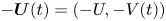 $-\boldsymbol {U}(t) = (-U, -V(t))$, constant in the horizontal direction, and sinusoidal in the vertical direction. We solve the incompressible Navier–Stokes equations, non-dimensionalized, in the rest frame of the lattice using the finite-difference method described in Part 1. The basic dimensionless parameters are
 \begin{equation} \frac{A}{L}, \quad Re_f = \frac{f L^2}{\nu}, \quad l_x = \frac{L_x}{L}, \quad l_y = \frac{L_y}{L},\quad U_L = \frac{U}{fL}, \end{equation}
with  $A$ the amplitude and
  $f$ the frequency of the vertical displacement corresponding to
  $V(t)$. We non-dimensionalize quantities using the plate length
  $L$ as the characteristic length, the flapping period
  $1/f$ as the characteristic time and the fluid mass density
  $\rho _f$ as the characteristic mass density. Here,
  $\nu$ is the kinematic viscosity of the fluid and
  $L_x$ and
  $L_y$ are the lattice spacings in the
  $x$ and
  $y$ directions, respectively.

Figure 1. (a) A rectangular lattice of plates. The computational domain is an  $L_x$-by-
 $L_y$ unit cell, shown with a dashed blue outline. (b) A rhombic lattice of plates. The computational domain is an
  $L_x$-by-
 $2 L_y$ double unit cell, shown with a dashed blue outline.
We refer to other important dimensionless parameters, combinations of those above
 \begin{equation} Re = \frac{4A f L}{\nu}, \quad Re_U = \frac{U L}{\nu}, \quad U_A = \frac{U}{fA}, \quad St = \frac{2}{U_A}. \end{equation}
Here,  $Re$ is the Reynolds number based on the mean vertical velocity of the foil on each half-stroke, while
  $Re_f$ can be considered a dimensionless frequency, because
  $\nu$ and
  $L$ are assumed fixed.
Given the net horizontal force on each plate  $F_x$ (due to viscous shear) and the net vertical force
  $F_y$ (due to pressure), we define the input power
  $P_{in}(t)$ and the Froude efficiency
  $\eta _{Fr}$
 \begin{equation} P_{in}(t) = \frac{V(t)}{fL} F_y; \quad {\tilde P}_{in}(t) = Re_f^3 P_{in}(t); \quad \eta_{Fr} = \frac{U\langle F_x(t) \rangle}{\langle P_{in}(t) \rangle}. \end{equation}
Here,  ${\tilde P}_{in}(t)$ is the input power non-dimensionalized with
  $\nu /L^2$ in place of
  $f$, for comparison across cases with different
  $f$ (since
  $L$ and
  $\nu$ are assumed fixed). The numerator and denominator of
  $\eta _{Fr}$ both acquire factors of
  $Re_f^3$ with the same change in non-dimensionalization, resulting in no change for
  $\eta _{Fr}$.
In Part 1, we established some of the main properties of an isolated flapping plate in an oncoming flow. We now discuss flows in the much larger space of doubly periodic lattices of flapping plates. We consider two types of lattices, rectangular and rhombic (diamond), shown in figure 1, also considered by Weihs (Reference Weihs1975); Daghooghi & Borazjani (Reference Daghooghi and Borazjani2015); Hemelrijk et al. (Reference Hemelrijk, Reid, Hildenbrandt and Padding2015); Park & Sung (Reference Park and Sung2018) and Oza, Ristroph & Shelley (Reference Oza, Ristroph and Shelley2019). Between these two lattices is the full range of two-dimensional (2-D) (oblique) lattices. We focus only on the two endpoint lattice types (rectangular and rhombic) because the remaining parameter space is already quite large (five-dimensional). For the rectangular lattice, we solve the flow in a single unit cell (figure 1(a), blue dashed-line rectangle) with periodic boundary conditions. For the rhombic case, we solve the flow in a domain consisting of two unit cells (figure 1(b), blue dashed-line rectangle), to observe when flow modes arise that are periodic on length scales longer than a single unit cell. We focus on time-periodic dynamics for the most part, because such states are generally reached within 5–30 flapping periods. The dynamics usually appears to be non-periodic at larger  $Re$ values, and may therefore require much longer run times to compute long-time averages with high accuracy. We generally avoid presenting time-averaged values for these cases except where noted explicitly in the text (e.g. for the average input power).
2. Examples of thrust–drag transitions and periodic flow states
Figure 2(a)–(d) shows the average horizontal force  $\langle F_x(t) \rangle$ versus normalized horizontal flow speed
  $U/fA = 2/St$ for a rectangular lattice of plates at
  $Re = 20$ and various
  $l_x$ and
  $l_y$ values. In the single-body case, the sidewall and upstream boundary conditions may cause numerical instabilities when vortices collide with these boundaries, i.e. when the oncoming flow speed is too small to advect vortices to the downstream boundary. This issue does not arise with doubly periodic boundary conditions, and the flow computations remain stable with small oncoming flow speeds, so unlike in figure 7(a) of Part 1, in figure 2(a)–(d) the curves can be computed down to zero
  $U/fA$. Panel (a) shows four curves with
  $A/L = 0.2$,
  $l_y = 1$ and
  $l_x$ ranging from 1.2 to 1.5 (labelled at right). The vertical gap is one plate length, but the horizontal gap is smaller, 0.2 to 0.5. Here,
  $\langle F_x \rangle$ initially increases with
  $U/fA$, so unlike a single flapping plate at this
  $Re$, zero velocity is a stable equilibrium here. After reaching a peak, each curve drops (sharply for
  $l_x = 1.2$, then more smoothly as
  $l_x$ increases), and then adopts a U-shape somewhat similar to that in the isolated-body case. For
  $l_x = 1.2$ to 1.4, there are three zero crossings (counting
  $U/fA = 0$), corresponding to three equilibria, two stable and one unstable, while at
  $l_x = 1.5$, the only equilibrium is the zero-velocity state. Panel (b) shows the same data with
  $l_y$ increased to 1.5. The darkest blue curve (
 $l_x = 1.2$) now has two sharp drops, between which the curve increases with
  $U/fA$. Near zero
  $U/fA$, the curve is dotted, indicating that the dynamics is non-periodic in this region, so for the averages on the dotted line there is some uncertainty (that we do not quantify here). At the last of these non-periodic cases (highest circled point), the time trace of
  $F_x(t)$ is shown in a small inset panel, with tick marks every flapping period along the horizontal axis. The graph of
  $\langle F_x(t) \rangle$ then drops sharply to the next point, also circled, at which the time trace becomes periodic with period 1. The dynamics remains 1-periodic as
  $\langle F_x(t) \rangle$ increases to the next circled point. Then
  $\langle F_x(t) \rangle$ drops sharply again, to a state that is 1/2-periodic, the fourth and final circled point on this curve. The curve then increases smoothly with further increases in
  $U/fA$. In this case, the sharp drops in the curve correspond to changes in periodicity, from non-periodic, to 1-periodic, to 1/2-periodic. We will discuss the corresponding flow structures below. The remaining curves in this panel, for
  $l_x = 1.3$ to 1.5, become increasingly smooth as
  $l_x$ increases, eventually resembling those in panel (a), but with an additional equilibrium for
  $l_x = 1.4$ and 1.5; zero velocity is unstable for these cases. Panel (c) shows the same quantities for
  $A/L$ increased to 0.5 and
  $l_y$ increased to 2, and a wider range of
  $l_x$ (labelled at right). The two inset panels show another example of the change in dynamics (from 4-periodic to 1/2-periodic) that accompanies a sharp drop in
  $\langle F_x \rangle$ at a particular
  $U/fA$. Panel (d) (
 $l_y = 3$) shows three more examples of changes from a 1-periodic to a 1/2-periodic dynamics that occur at sharp drops in
  $\langle F_x \rangle$. Panels (c,d) indicate a transition with respect to
  $l_x$ as well. For
  $l_x$ near 1 (blue curves), the plates experience drag at small
  $U/fA$. At larger
  $l_x$ (green and yellow curves), more complex variation of
  $\langle F_x \rangle$ is seen at small
  $U/fA$ including thrust. By counting the numbers of zero crossings of these curves (including
  $U/fA = 0$), we obtain the number of equilibrium states, and show the totals as coloured patches in figure 2(e–g), for
  $A/L = 0.2$ (e), 0.5 (f) and 0.8 (g). In the dark blue regions
  $U/fA = 0$ is the only equilibrium, and there is no net locomotion. This is the case at smaller
  $l_y$ in most cases, and some larger
  $l_y$ values at the largest
  $A/L$ (panel (g)). The close vertical stacking of adjacent bodies tends to suppress vortex formation and thrust generation, as we will illustrate later. In the light blue regions, there are two equilibria:
  $U/fA = 0$ is unstable and there is a stable self-propelled state, as in the isolated-body case. Examples are given by the yellow lines in panels (c,d), which represent the closest approximation to the isolated body among these cases (
 $l_x$ and
  $l_y$ are largest). However, the body might not be well approximated as isolated in some cases; there can be significant flow interactions across the periodic unit cell, particularly at
  $A/L = 0.5$ and 0.8. The yellow regions in figure 2(e–g) have three or more equilibria, and these generally correspond to small
  $l_x$ and large
  $l_y$. The interactions between adjacent bodies’ edges are strongest here, and lead to a variety of flow modes (and dynamics, indicated by the insets we have discussed) that are sensitive to small changes in
  $U/fA$ and the other parameters. At the largest
  $A/L$ (panel (g)), these states are suppressed by the larger amplitude of motion, which tends to suppress interactions between vortices shed by horizontally adjacent plates.
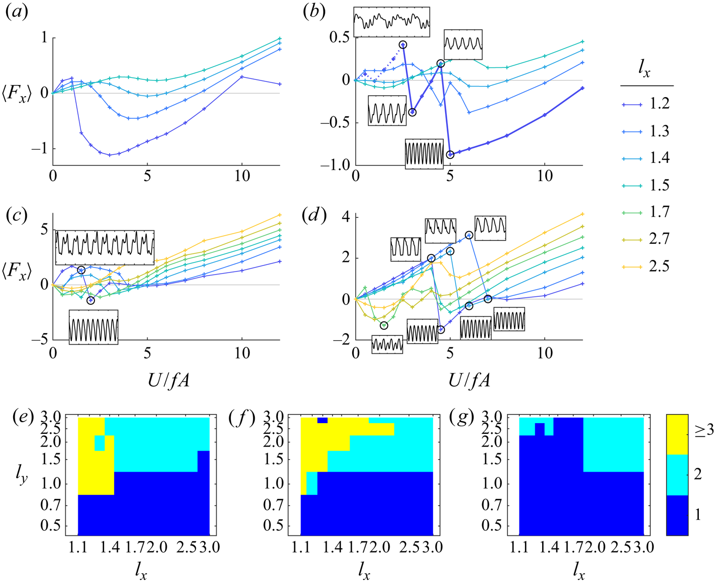
Figure 2. Average horizontal force  $\langle F_x(t) \rangle$ versus normalized horizontal flow speed
  $U/fA = 2/St$ for
  $Re = 20$ and various
  $l_x$ and
  $l_y$ values. In panels (a)–(d), each line plots
  $\langle F_x(t) \rangle$ versus
  $U/fA$ for various
  $l_x$, listed at right. Specific values of
  $A/L$ and
  $l_y$ are chosen for each of the panels; (a)
  $A/L = 0.2$,
  $l_y = 1$, (b)
  $A/L = 0.2$,
  $l_y = 1.5$, (c)
  $A/L = 0.5$,
  $l_y = 2$, (d)
  $A/L = 0.5$,
  $l_y = 3$. (e–g) For various (
 $l_x$,
  $l_y$) pairs, the number of equilibrium states (
 $U/fA$ with
  $\langle F_x(t) \rangle = 0$), for
  $A/L = 0.2$ (e), 0.5 (f) and 0.8 (g).
Figure 3 shows examples of the flows near the sudden drops in  $\langle F_x \rangle$. In figure 2(b), four circled data points are shown, bracketing two sudden drops in
  $\langle F_x \rangle$. Corresponding flows, at two instants spaced 1/2 of a flapping period apart, are shown by the four pairs of panels in the purple box of figure 3. Panels (a,b) show the flow at
  $U/fA$ slightly below the first circled data point, in a quasi-periodic state giving drag. In panel (a), the upward flow through the thin gap between adjacent plate edges produces an asymmetric vortex dipole. In panel (b), a 1/2-period later, the downward flow produces a similar asymmetric dipole. In both cases, although the net flow is rightward, the vortices on the leftward sides of the dipoles are larger. Panels (c,d) show the corresponding flows at the second circled point in figure 2(b), after the first sudden drop in
  $\langle F_x \rangle$, to a state of net thrust. Again, two vortex dipoles are produced on each half-cycle, but now the upward dipole curves rightward (downstream), and the rightward (blue) vortex is larger. However, the downward dipole is still roughly symmetric. Panels (e,f) show the corresponding flows at the third circled point in figure 2(b). The downstream flow is larger, and net drag is obtained. In panel (e), the upward dipole is more symmetric, similar to the downward dipole in panel (d), and the downward dipole in panel (f) is curved downstream, like that in panel (c). Panels (g,h) show the flows at the fourth circled point in figure 2(b), after the second sudden transition from net drag to net thrust. Now both dipoles are curved rightward. Panels (g,h) also show a flow state that is up–down symmetric after a 1/2-period. Consequently,
  $F_x(t)$ (inset next to fourth circle in figure 2b) is 1/2-periodic – the horizontal force is the same on the up and down strokes. By contrast, the first, second and third flow states were not up–down symmetric, and
  $F_x(t)$ was 1-periodic in each case. A similar phenomenon occurs at the sudden drop in
  $\langle F_x \rangle$ accompanied by the insets in figure 2C;
  $F_x(t)$ transitions from 4-periodic to 1/2-periodic in the insets. Flow snapshots are shown in the green box of figure 3; panels (i)–(j) for the first inset of figure 2(c), and panels (k)–(l) for the second. In panels (i–j), the vortex dipoles are not up–down symmetric after a 1/2-period, and the upstream member of each vortex pair is larger. In panels (k–l), the dipoles are up–down symmetric, and the downstream vortices are larger. A similar phenomenon also occurs at each of the three sudden drops in
  $\langle F_x \rangle$ highlighted by circles in figure 2(d). The corresponding flow transitions, from up–down asymmetric to symmetric, are shown in figure 19 in appendix A. The general phenomenon then is that sudden changes from drag to thrust can occur when
  $l_x$ is close to 1, when the dipole jets on each half-stroke switch from upstream to downstream orientations. As
  $l_x$ increases to larger values, the curves may become smoothed versions of those with sharp drops, e.g. in figure 2(a). Eventually, at large enough
  $l_x$, the vortex shedding pattern changes qualitatively, from a dipole between adjacent leading and trailing edges to a single dominant vortex that interacts with previously shed vortices in the wake, e.g. the reverse von Kármán street.

Figure 3. Flow states that accompany the sudden drops in  $\langle F_x \rangle$ highlighted in figure 2(b) (purple box) and (c) (green box). Panels (a)–(b) and (c)–(d) show vorticity snapshots 1/2-period apart, before and after the first sudden drop in
  $\langle F_x \rangle$ shown by circles in figure 2(b). Panels (e)–(f) and (g)–(h) correspond to the second drop in figure 2(b). The green box (i)–(l) shows the flow state transition for the drop in figure 2(c). The colour bar limits are
  $\pm \omega _{s}$ where
  $\omega _{s} = 3$ (a)–(h) or 3.5 (i)–(l).
Figures 2, 3 and 19 have shown that for  $l_x$ near 1,
  $F_x(t)$ can sharply change from 1-periodic (or 4-periodic) to 1/2-periodic at certain oncoming flow speeds. Figure 4 shows further examples of the diversity of periodic
  $F_x(t)$ that can occur when
  $l_x$ is near 1. Panels (a,b) show 1/2-periodic
  $F_x(t)$, the first roughly sinusoidal, the second far from it. Panel (c) shows a 1-periodic state. Panels (d,e) show 1.5-periodic states, with repeated features highlighted in red. Panel (e) can be regarded as a perturbation of a 1/2-periodic state. Panels (f,g) are 2-periodic states with repeated features highlighted in green; panel (f) is nearly 1/2-periodic, while panel (g) is nearly 1-periodic. Panel (h) shows that the dynamics can switch between different nearly periodic states over long periods of time. The blue regions last for 2.5 periods, while the red regions are nearly 3-periodic, and their recurrences (with slight changes) do not follow a simple pattern up to
  $t = 30$. Panel (i) shows the 4-periodic state of figure 2(c), top inset, with repeated features highlighted in orange; the state is nearly 1-periodic. Panel (j) shows a non-periodic state that nonetheless has recurrent downward spikes (in red) near certain times that are spaced by multiples of 0.5:
  $t = 3.2$, 5.7, 7.2, 8.2, 10.2 and 11.7.

Figure 4. Examples of  $F_x(t)$ exhibiting various types of periodicity when
  $l_x$ is close to unity. All occur for rectangular lattices with
  $Re = 20$. (a)
  $A/L = 0.2$,
  $l_x = 1.2$,
  $l_y = 1$,
  $U/fA = 1$; (b)
  $A/L = 0.5$,
  $l_x = 1.2$,
  $l_y = 1$,
  $U/fA = 1$; (c)
  $A/L = 0.5$,
  $l_x = 1.2$,
  $l_y = 3$,
  $U/fA = 1$; (d)
  $A/L = 0.8$,
  $l_x = 1.1$,
  $l_y = 2$,
  $U/fA = 0.5$; (e)
  $A/L = 0.8$,
  $l_x = 1.1$,
  $l_y = 1$,
  $U/fA = 4.5$; (f)
  $A/L = 0.8$,
  $l_x = 1.2$,
  $l_y = 1$,
  $U/fA = 12$; (g)
  $A/L = 0.5$,
  $l_x = 1.3$,
  $l_y = 2$,
  $U/fA = 3.5$; (h)
  $A/L = 0.2$,
  $l_x = 1.2$,
  $l_y = 2$,
  $U/fA = 1$; (i)
  $A/L = 0.5$,
  $l_x = 1.2$,
  $l_y = 2$,
  $U/fA = 1$; (j)
  $A/L = 0.8$,
  $l_x = 1.1$,
  $l_y = 2$,
  $U/fA = 10$.
Figure 5 shows examples of flows for which  $F_x(t)$ has a period larger than unity. Panels (a–d) show snapshots, a 1/2-period apart, that correspond to figure 4(d). Panel (a) shows an upward dipole, followed in panel (b) by a downward dipole. Panel (c) shows a smaller upward dipole, and then panel (d) is a mirror image of panel (a) (with opposite-signed vorticity). The next two snapshots (not shown) would be mirror images of panels (b,c), followed by a return to panel (a). Thus
  $F_x(t)$ has period 1.5 and the flow has period 3. Panels (e)–(i) show a flow with period 2, and with
  $F_x(t)$ of period 2. The upward, rightward curving dipole in panel (e) is followed by a straighter downward dipole in panel (f). The dipole in panel (g) is more curved than in panel (e), while that in panel (h) is similar to that in panel (f). With panel (i), the flow returns to panel (e). This flow is a more slightly perturbed version of a 1-periodic flow than the flow in panels (a)–(d), as are many of the
  $n$-periodic flows we have observed.

Figure 5. Flows exhibiting different periodicities. (a)–(d) Snapshots spaced by a half-period corresponding to  $F_x(t)$ in figure 4(d). Panel (d) is essentially a mirror image of panel (a). (e)–(i) Snapshots spaced by a half-period for a 2-periodic flow (
 $Re = 20$,
  $A/L = 0.5$,
  $l_x = 1.3$,
  $l_y = 2$ and
  $U/fA = 3$). The colour bar limits are
  $\pm \omega _{scale}$ where
  $\omega _{scale} = 300$ (a–d) or 100 (e–i).
3. Transitions from periodic to non-periodic flows as parameters are varied
We have studied examples of  $F_x(t)$ and flows with different periods, mainly for
  $l_x$ close to 1. More broadly, there is a gradual trend towards non-periodicity at certain parameter values. For
  $Re = 20$, and three different
  $A/L$ (0.2 (a), 0.5 (b) and 0.8 (c)), we plot circles in figure 6 where
  $F_x(t)$ deviates from 1-periodicity by the following measure. We compute the averages of
  $F_x(t)$ over the last eight half-periods of
  $V(t)$, during
  $t = 11$ to 15. We split the eight values into two sets of four, one for the first half-period of
  $V(t)$ and the other for the second half-period. We sum the standard deviations over the two sets and normalize by
  $\frac {1}{4}\int _{11}^{15} |F_x(t)| \, \textrm {d} t$ (an average magnitude of
  $F_x$). Where the resulting value is greater than 0.01, we plot circles in figure 6. The 0.01 threshold is somewhat arbitrary, but is chosen with certain considerations in mind. The flapping motion imposes a strong 1-periodic component in all flows, so a threshold of 0.1, say, would classify some non-periodic
  $F_x(t)$ as periodic. A threshold much smaller than 0.01 would miss some
  $F_x(t)$ that have almost but not completely converged to periodic near
  $t = 15$. The circles occur predominantly at large
  $l_y$, and more often at small
  $l_x$, though they are also found at large
  $l_x$. The reason is that the close spacing of plates at small
  $l_y$ tends to suppress complex vortical structures, and leads to more laminar, periodic flows. As we have seen, small
  $l_x$ leads to formation of thin dipole jets with sharp concentration of vorticity, and complicated non-periodic dynamics can result. Many of these cases occur at small oncoming velocity (large
  $St$), reflected in the larger number of small blue circles across the panels. As we have seen for the isolated body, above a certain flow speed, a reverse von Kármán street tends to form, in many cases due to merging or other regular interactions between the leading and trailing edge vortices. The larger number of yellow circles at
  $A/L = 0.2$ (panel (a)) is perhaps because at a given
  $U/fA$,
  $U/fL$ is smaller in panel (a), so in a given flapping period, vortices do not move as far downstream relative to the plate length in this case, leading to a more complicated dynamics. Also,
  $Re$ is constant (20) in all three panels, so
  $Re_f$ decreases from left to right. To the extent that viscous regularizing effects are more controlled by
  $Re_f$, they are increased moving from left to right. The corresponding data for the rhombic lattice are shown in figure 20 in the appendix, and shows similar trends but with additional non-periodic states at smaller
  $l_y$.

Figure 6. Circles show parameter values where a measure of the deviation of  $F_x(t)$ from time-periodicity unity (described in the main text) exceeds 0.01, for a rectangular lattice of plates with
  $Re = 20$. Values of
  $A/L$ are 0.2 (a), 0.5 (b) and 0.8 (c). Values of
  $St$ (note
 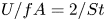 $U/fA = 2/St$) are labelled by circle size and colour (key listed at right). Circles are centred at the corresponding values of
  $l_x$ and
  $l_y$.
Figure 7 shows information about the types of periodic states that occur in parameter space, some corresponding to the  $F_x(t)$ and flows shown in figures 2–5. The panels again show states at
  $A/L = 0.2$ (a), 0.5 (b) and 0.8 (c). Within each panel are a set of boxes (black outlines), each centred at the corresponding
  $(l_x, l_y)$ pair. Each box contains a set of smaller squares, each for a different value of
  $St$ ranging from 0.17 to 4 (listed at lower right, note
  $U/fA = 2/St$). The grey squares correspond to
  $F_x(t)$ with period 0.5. The coloured squares correspond to period 1 but not period 0.5, i.e. flows that are not up–down symmetric. For these flows only, we use the colours to label the
  $St$ value. The black squares are for non-periodic
  $F_x(t)$, the cases shown by circles in figure 6. White spaces lie within some of the boxes because not all parameter combinations were computed, but the overall pattern is not altered by these omissions. At
  $Re = 20$, most squares are grey, so most flows are up–down symmetric. The coloured squares (1-periodic states) occur mainly at smaller
  $l_x$ and larger
  $l_y$. They are most prevalent at the intermediate
  $A/L$ (panel (b)), and there they occur at large
  $St$, i.e. smaller
  $U/fA$. We have also noted a few cases of
  $F_x(t)$ with longer periods: 1.5 (red crosses), 2 (red circles) and 4 (red square), all of which occur at small
  $l_x$. In general, the period-1 and longer-period states occur near the non-periodic states (black squares), so the former may be intermediaries in the transition from 1/2-periodic to non-periodic states as the parameters are varied to allow more disordered flows.

Figure 7. Flows at  $Re = 20$ for a rectangular lattice, classified by type of periodicity, with
  $A/L = 0.2$ (a), 0.5 (b) and 0.8 (c). Each box shows data for a certain (
 $l_x$,
  $l_y$) pair that is located at the box centre, and contains a set of smaller squares, each for a different value of
  $St$ ranging from 0.17 to 4 (listed at right, note
  $U/fA = 2/St$). The grey boxes correspond to
  $F_x(t)$ with period 0.5. The coloured boxes correspond to period 1 but not period 0.5, i.e. flows that are not up–down symmetric. For these flows only, we use the colours to label the
  $St$ value. The black boxes denote non-periodic
  $F_x(t)$.
Figure 8 shows the same quantities when the lattice is changed from rectangular to rhombic. The general trend of  $F_x(t)$ with increasing period or non-periodic at smaller
  $l_x$ and larger
  $l_y$ is basically preserved. Compared to the rectangular lattice data, there are more 1-periodic and non-periodic
  $F_x(t)$ at small
  $l_y$. This is perhaps because there is more
  $y$-distance between adjacent bodies for the rhombic lattice than for a rectangular lattice at the same
  $l_y$, allowing for more complex flows.

Figure 8. Flows at  $Re = 20$ for a rhombic lattice, classified by type of periodicity, with
  $A/L = 0.2$ (a), 0.5 (b) and 0.8 (c). Each box shows data for a certain (
 $l_x$,
  $l_y$) pair (at the box centre), and contains a set of smaller squares, each for a different value of
  $St$ ranging from 0.17 to 4 (listed at right, note
  $U/fA = 2/St$). The grey boxes correspond to
  $F_x(t)$ with period 0.5. The coloured boxes correspond to periodicity unity but not periodicity 0.5, i.e. flows that are not up–down symmetric. For these flows only, we use the colours to label the
  $St$ value. The black boxes denote non-periodic
  $F_x(t)$.
4. Large  $l_y:$ approximately 1-D tandem lattices

One important limiting case is the large- $l_y$ limit. Here the configuration consists of well-separated 1-D arrays of flapping plates. The flows around the 1-D arrays are essentially the same for the rectangular and rhombic lattices. Figure 9 presents an example of such a flow, at
  $l_x = 2$ and
  $l_y = 3$. Figure 9(a–f) is a sequence of vorticity snapshots during the half-period of upward flow relative to the plates, for a rectangular lattice. The six snapshots are spaced apart by 0.1 in
  $t$. The positive (red) vortices below the plates in the first panel, shed from the leading edge on the previous half-period, now merge with positive vorticity shed from the trailing edge during this half period. This is a case of relatively high Froude efficiency. The main difference from an isolated plate is the close interaction between the vortices shed at the leading and trailing edges of adjacent bodies, and the blue vortices are above the orange vortices, the opposite of the reverse von Kármán streets of figure 4 and 5 of Part 1, and more similar to a regular von Kármán street (albeit with plates among the vortices). The lower row shows the same flow for a rhombic lattice of plates. The flow is almost the same, because there is little interaction between vertically adjacent rows. A double layer of weak vorticity (yellow–green region) separates the vortex arrays of each row. In this region, the flow velocity is approximately uniform, with vertical flow speed equal to the average vertical flow speed, and horizontal flow speed approximately twice the average horizontal flow speed. The horizontal flow speed in the plate/vortex array is both positive and negative, and much smaller in magnitude.

Figure 9. Six vorticity snapshots spaced by 0.1 in  $t$ during the half-period of upward flow, for rectangular (a–f) and rhombic (g–l) lattices. The parameters are
  $A/L = 0.5$,
  $l_x = 2$,
  $l_y = 3$,
  $Re = 70$ and
  $U/fA = 7$.
We now show examples of how the large- $l_y$ flows change as
  $l_x$ and
  $A/L$ are varied, in figure 10. We choose
  $Re = 20$ and
  $U/fA = 3$ (large enough that regular vortex arrays may be generated, and small enough that thrust may occur). In figure 10(a–d),
  $A/L = 0.2$. Moving left to right, as the gap between adjacent plates increases, the flow changes from a dipole to a vortex street. At far right, the trailing edge vortices interact more with the previously shed trailing edge vortex than with that shed at the leading edge of the adjacent plate. There is mean thrust for the flows in panels (a,b), approximately zero thrust in panel (c), and small net drag in panel (d). In figure 10(e–h),
  $A/L = 0.5$, there is again a transition from dipole jets to a vortex street, with larger vortices now. Now there is also small but noticeable coupling between adjacent rows of plates. Instead of uniform flow, in the first three panels there are bands of nearly constant non-zero vorticity above and below the vortex arrays (yellow–green region in panel (e) that becomes blue–green in panels (f,g)). These are shear flows with
  $u$ nearly linear with respect to
  $y$ and
  $v$ nearly constant. They differ from those that would be seen with an isolated flapping body, and therefore, unlike the flows in the first row, they would be altered for larger
  $l_y$ values. In the second row, only the third column corresponds to a state of mean thrust. In the third row,
  $A/L = 0.8$, only the first column is a state of mean thrust. It is not obvious from the form of the vortex dipole why mean thrust occurs, but there are noticeable differences with the orientation of the dipole in the second panel. Again there are linear shear zones above and below the dipole jets. In the fourth column, same-signed vortices are almost linked vertically now in contiguous bands of same-signed (but very non-uniform) vorticity. Now the plates are coupled strongly to both vertical and horizontal neighbours through the flow.

Figure 10. Flow snapshots with  $l_x = 1.2$, 1.5, 2 and 3 (left to right columns) and
  $A/L = 0.2$, 0.5 and 0.8 (top to bottom rows). The other parameters are:
  $Re = 20$,
  $U/fA = 3$,
  $l_y = 3$. The colour bar limits are
  $\pm \omega _{s}$ where
  $\omega _{s} = 30$ (a), 20 (b), 10 (c,d), 100 (e), 50 (f), 30 (g), 10 (h), 150 (i), 50 (j), 30 (k) and 10 (l).
5. From small to large $l_y$ at $l_x = 2$


We have shown examples of flows with  $l_y$ fixed and
  $l_x$ from small to large. We now reverse the parameters, i.e. hold
  $l_x$ fixed at 2 (an intermediate value), and vary
  $l_y$ from small to large. Figure 11 shows examples of vorticity fields at instants of upward (and as usual, rightward) flow. Since
  $l_y$ may be small, there can be significant differences between rectangular and rhombic lattice flows and we show both. The differences are most pronounced at the smallest
  $l_y$. In panels (a) and (c) (
 $l_y = 0.2$ and
  $U/fA = 3$ and 7, respectively), the flow through the rectangular lattice is approximately horizontal Poiseuille flow between the vertical neighbours (away from the plate end regions), and unidirectional vertical flow in the space between horizontal neighbours. Most of the vertical mass flux occurs in these vertical channels, and the flow past the plate edges is relatively weak. These small-
 $l_y$ flows result in a net drag force, almost constant in time, that of the Poiseuille flow between the plates. The corresponding rhombic lattice flows (b,d) are much more complex. The plates now cover the full horizontal extent of the flow field, so the entire flow is forced through the small gaps between the interleaving plate edges. Consequently, much stronger vorticity is generated at the plate edges. This flow results in a net thrust force, is not temporally periodic but
  $F_x(t)$ has a strong 1/2-periodic component, and is also not spatially periodic on the scale of a single unit cell (i.e. containing a single plate), but of course is periodic on the scale of a double unit cell by the definition of the periodic boundaries (the blue dashed-line rectangle in figure 1b). This can be seen by examining the flows below the right edges of the plates. There is a small blue vortex below the top plates’ right edges, but larger blue regions in (b,d) (displaced rightward in d) below the middle plates’ right edges. Increasing
  $l_y$ to 0.5, the rectangular lattice flows (e,g) deviate more from Poiseuille flow, while the rhombic lattice flows (f,h) become smoother. Panel (f), at lower
  $U/fA$, is still a temporally non-periodic flow, but closer to spatially periodic on the scale of the unit cell than panels (b) or (d). The flow in panel (h) is both temporally periodic and spatially periodic on the unit cell scale. Again, both rectangular lattice flows generate net drag, while the rhombic lattice flows generate net thrust. Increasing
  $l_y$ to 1, both rectangular flows (i,k) again generate drag, although (i), at lower
  $U/fA$, is close to zero net drag. Of the rhombic lattice flows (j,l), only j generates thrust, but with relatively high Froude efficiency (0.04), much higher than in panel (f) due both to increased thrust and decreased input power. Unlike the rectangular lattice, the rhombic lattice geometry allows a strong vortex dipole to form at this
  $l_y$ (panel (j)), involving a positive (red) vortex at the right edges of the middle plates and a negative vortex (blue) at the left edges of the bottom plates, which probably underlies efficient thrust generation. Increasing
  $l_y$ to 2, the rectangular lattice has the first occurrence of a state of net thrust in this figure, at low
  $U/fA$ (m) but not high
  $U/fA$ (o). The rhombic lattice has a state of net thrust at both speeds ((n,p)). At the largest
  $l_y = 3$, the rectangular (q,s) and rhombic (r,t) flows are similar as discussed below figure 9; both pairs generate net thrust with only small differences in their magnitudes and the corresponding Froude efficiencies. To summarize, for the rectangular lattice, only net drag occurs below a moderate
  $l_y$. For the rhombic lattice, by contrast, thrust can occur at very small
  $l_y$, although the flows are non-periodic and the Froude efficiency is low. We can also see that the rhombic lattice flows converge to spatially periodic on the unit cell scale as
  $l_y$ becomes large, which correlates with the convergence to temporal periodicity. By computing the relative error in unit cell periodicity for a number of other flows (76 in all) at various parameters, we find that unit cell periodicity correlates with temporal periodicity in general. Both are more prevalent when
  $Re$ is small, and when
  $l_x - 1$ is not very small. However, there are examples of one without the other and vice versa. Therefore, in a large lattice of plates of plates at sufficiently large
  $Re$, the flow would be expected to deviate from the periodic lattice model with unit cell periodicity. However, in most cases considered in this paper, the deviation is not very large.

Figure 11. Flow snapshots with  $l_x = 2$ and various
  $l_y$: 0.2 (a–d), 0.5 (e–h), 1 (i–l), 2 (m–p) and 3 (q–t). Within each group of four consecutive panels, the first two are for
  $U/fA = 3$ (a–b, e–f, i–j, etc.) and the second are for
  $U/fA = 7$. Within each of these two pairs of panels, the first is a rectangular lattice (a, c, e, g, etc.) and the second is a rhombic lattice. In all cases,
  $Re = 70$ and
  $A/L = 0.5$. The values of vorticity on the contours are labelled on the colour bar at lower right. The colour bar limits are
  $\pm \omega _{s}$ where
  $\omega _{s} = 1000$ (bd), 150 (f,h) and 50 in all other cases (including all rectangular lattices).
6. Froude efficiencies and self-propelled speeds across parameters
We have discussed some examples of plate–plate interactions that lead to thrust generation in certain 1-D slices through parameter space: small to large  $l_x$ at intermediate and large
  $l_y$ (figures 3, 10 and 19), and small to large
  $l_y$ at intermediate
  $l_x$ (figure 11). In the
  $l_x$–
 $l_y$ plane, we present in figure 12 contour plots of Froude efficiency at
  $Re = 20$, small enough that most flows are time periodic. Contours are plotted for rectangular (a–c) and rhombic lattices (d–f), with
  $A/L = 0.2$ (a,d), 0.5 (b,e) and 0.8 (c,f). Comparing panels (a) and (d), the contour lines are very similar for
  $l_y$ above 2. At this
  $A/L$ and large
  $l_y$, there is little interaction between different horizontal rows of plates, so the lattice type makes little difference, as in figure 9. Below
  $l_y = 2$, the contour lines in A bend sharply leftward, and efficient thrust is only obtained by the rectangular lattice for
  $l_x$ near 1, if at all. At smaller
  $l_y$, the rhombic lattice is more efficient, and yields net thrust down to
  $l_y = 0.2$ (orange line in panel (d)), as noted previously for
  $Re = 70$. Increasing
  $A/L$ to 0.5 (b,e), there is an overall decrease in peak Froude efficiency by about a factor of 2 for both lattice types. The contour lines in B deviate more at larger
  $l_y$ from those in (e) now, as the increased
  $A/L$ results in more interaction between different horizontal rows of plates. For both lattice types, the peak Froude efficiency occurs at much larger
  $l_x$. For larger
  $A/L$, the vorticity has a larger vertical extent. For an isolated plate, figure 8(a) of Part 1 shows that
  $U/fA$ should be kept roughly constant as
  $A/L$ increases, for peak efficiency. This means that
  $U/fL$ increases. Thus the vortices are more spread out horizontally, and it is reasonable that the plates should be more spread out to interact with vortices efficiently. The trends continue in panels (c,f) of figure 12: further reductions in peak Froude efficiency, that occur at still larger
  $l_x$. In all cases, net thrust is obtained down to lower
  $l_y$ by the rhombic lattice. This is shown by the zero contours, extending lower in the bottom row than in the top row.
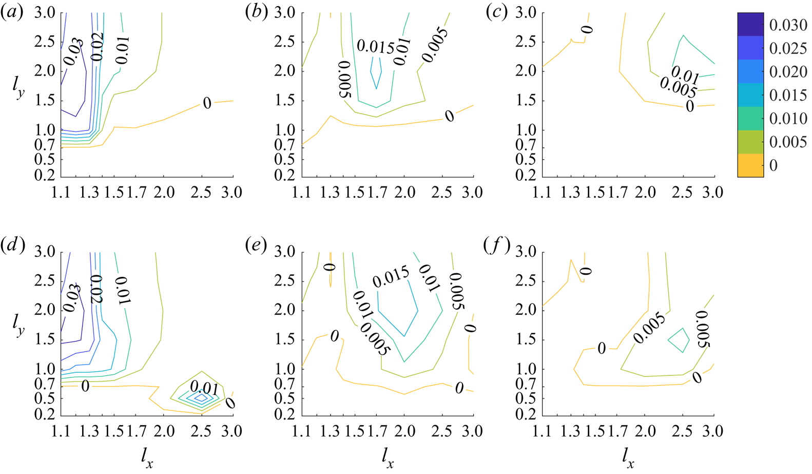
Figure 12. Contours of Froude efficiency for rectangular (a–c) and rhombic lattices (d–f) at  $A/L$ = 0.2 (a,d), 0.5 (b,e) and 0.8 (c,f).
Another measure of performance is the maximum self-propelled speed  $U_{SPS}/fA$ achieved by the lattice. These data are presented in figure 13 for the rectangular (a–c) and rhombic (d–f) lattices, at
  $A/L = 0.2$, 0.5, and 0.8 (left to right columns). In all panels, the highest speeds are obtained at the smallest
  $l_x$, where vortex dipole formation leads to strong forces on the plates. The much smaller speeds at larger
  $l_x$ may be partly due to the relatively small
  $Re$, which leads to substantial diffusion of vortices as they move over a larger lattice length scale. As in figure 12, the two lattices’ speeds agree better at larger
  $l_y$; the rhombic lattice achieves propulsion at smaller
  $l_y$ than the rectangular lattice, with moderate to large
  $l_x$. An example is the local maximum in panel (d) at
  $l_x = 2.5$ and
  $l_y = 0.5$, close to the parameters for the flow in figure 11(f) but at lower
  $Re$. In panels (b,e), there is a small band where
  $l_x = 1.3$ and
  $l_y = 2.5$ and 3 where the speed is greatly reduced or zero. The reason is not obvious, but may reflect a particular aspect of dipole formation at this value of
  $Re$.
$Re$.

Figure 13. Comparison of self-propelled speeds for rectangular (a–c) and rhombic (d–f) lattices at  $Re = 20$ and
  $A/L$ = 0.2 (a,d), 0.5 (b,e) and 0.8 (c,f).
When we increase  $Re$ much above 20, more flows are non-periodic up to
  $t = 30$, and a contour plot of Froude efficiency like figure 12 would require much longer simulations to achieve reliable long-time averages. Therefore, for higher
  $Re$, we present data only for cases that meet a threshold for periodicity. We use the same criterion described in figure 6, but increase the threshold from 0.01 to 0.08. Even at this larger threshold,
  $F_x(t)$ is close to periodic. The larger threshold allows us to present more values, and observe the general trends more easily. These trends are not very sensitive to the particular threshold chosen (0.08). Figure 14 expands upon figure 13 by presenting peak Froude efficiency values for three
  $Re$: 70 (a–c), 40 (d–f) and 10 (g–i), with the same
  $A/L$: 0.2, 0.5 and 0.8 (left to right columns). We do not use contours now because in many cases,
  $F_x(t)$ is non-periodic for all
  $U/fA$, and these are shown by grey boxes. If at a given choice of parameters there are
  $U/fA$ such that
  $F_x(t)$ meets the criterion for periodicity, the colour of the corresponding box denotes the peak Froude efficiency among the periodic cases, and the values are shown by the colour bars at right. The box colouring is solid or dotted if the peak value is obtained with a rectangular or rhombic lattice, respectively. The white boxes are cases where there are periodic flows, but all such flows yield net drag. One basic trend is the increasing non-periodicity of flows with
  $Re$: there are no grey boxes at
  $Re = 10$, some at
  $Re = 40$ and more at
  $Re = 70$. Non-periodicity is most common at small
  $l_x$, where the most intense vortex dipoles are created. At
  $Re = 70$, non-periodicity is more common at smaller
  $A/L$, where
  $Re_f$ is larger. At
  $Re = 10$ (figure 14g–i), the highest efficiency states are found at the smallest
  $l_x$, which are taken as small as 1.02; periodic flows are obtained nonetheless due to the small
  $Re$. Consistent with figure 12, efficiency usually drops as
  $A/L$ increases (from left to right). This is particularly true in figure 14(g–i), and can be seen in the change of green boxes to blue or white moving from (g) to (h) and then to (i). In figure 14(d–f) the same trend is shown by the decrease in the number of yellow boxes from (d) to (e) and then to (f). There are exceptions, however. For example, at
  $Re = 40$ and
  $(l_x, l_y) = (2.5, 1)$, peak efficiency is larger at
  $A/L = 0.8$ than
  $A/L = 0.2$. At
  $Re = 40$ (figure 14d–f), the most efficient periodic flows are obtained at much larger
  $l_x$ than for
  $Re = 10$. This is partly because many flows at smaller
  $l_x$ are non-periodic at
  $Re = 40$, however. At
  $Re = 40$ and 70 (figure 14a–c), the basic trends of figure 12 are mostly preserved: rhombic lattice flows are most efficient at small
  $l_y$, rectangular lattice flows are usually more efficient at large
  $l_y$, and peak efficiencies move to larger
  $l_x$ as
  $A/L$ becomes larger (moving rightward). Where the boxes are solid (typically at larger
  $l_y$), the peak efficiencies of the rectangular lattices are higher than those of the rhombic lattices, but only slightly. A possible reason for the slight advantage is that the plates in the rectangular lattice are vertically aligned, so they do not block the flow as much as the rhombic lattice does. Thus the input power is somewhat less, but the thrust forces are similar assuming the shear stresses on the plates are similar at large
  $l_y$. Previous models and computations (Weihs Reference Weihs1975; Hemelrijk et al. Reference Hemelrijk, Reid, Hildenbrandt and Padding2015; Oza et al. Reference Oza, Ristroph and Shelley2019) have reported an efficiency advantage for rhombic lattices, which we also find, at smaller
  $l_y$ typically. In general, as
  $Re$ increases in figure 14, so does peak Froude efficiency, from about 0.007 at
  $Re = 10$ to 0.033 at
  $Re = 20$ (from data in figure 12) to 0.055 at
  $Re = 40$, to 0.07 at
  $Re = 70$. As
  $Re$ increases above 10, fewer and fewer states are periodic, so these should be regarded as conservative lower bounds for the true peak Froude efficiencies, ones that include long-time averages of non-periodic flows.

Figure 14. Peak Froude efficiencies at  $Re = 70$ (a–c), 40 (d–f) and 10 (g–i), for
  $A/L = 0.2$ (a,d,g), 0.5 (b,e,h) and 0.8 (c,f,i). Grey boxes indicate that flows were non-periodic across
  $U/fA$. White boxes indicate that flows were periodic at some
  $U/fA$, but these only produced net drag. Coloured boxes indicate peak Froude efficiency magnitude (shown by colour bars at right) where periodic flow(s) that produced net thrust occurred. The colour field is solid or dotted if the peak was obtained with a rectangular or rhombic lattice, respectively. Each box is centred at the corresponding
  $(l_x, l_y)$ value, except the boundary boxes, where the value is given at the corresponding boundary edge.
We have shown in figure 14 how the maximum of the Froude efficiency over  $U/fA$ varies with respect to
  $Re$,
$Re$,  $A/L$,
  $l_x$ and
  $l_y$ for flows that are periodic or almost periodic. In figure 15 we replot the data from figure 14, adding the
  $Re = 20$ case, and showing both
  $\langle {\tilde P}_{in} \rangle$ and
  $\eta _{Fr}$ simultaneously. Thus, the four rows from top to bottom correspond to
  $Re = 70$, 40, 20 and 10, while the three columns from left to right have
  $A/L = 0.2$, 0.5 and 0.8. This figure allows us to identify which configurations are effective at different input power budgets, and describe the Pareto frontier for this set of data. In each panel we plot the data for rectangular lattices with small squares, with convex hull shown as a solid black line. The data for rhombic lattices are small diamonds with convex hull shown as a dashed black line. For each data point, the outline colour gives the value of
  $l_x$ and the interior colour gives the value of
  $l_y$ (listed at right). In each panel we also plot, at the panel's values of
  $Re$ and
  $A/L$,
  $\langle {\tilde P}_{in} \rangle$ and
  $\eta _{Fr}$ for an isolated body. This is shown with a red cross, or if there is no thrust for the isolated body at any of the
  $U/fA$ tested, the panel has a red outline. At the lowest two
  $Re$ (figure 15g–l),
  $\eta _{Fr}$ for the isolated body is zero or much smaller than for the lattices. The value of
  $\langle {\tilde P}_{in} \rangle$ for the isolated body is at the lower end of the range of lattice values, near the values for the largest
  $l_x$ and
  $l_y$. Panel (j) is a somewhat special case, as the large-
 $l_x$ lattice values did not yield thrust, but the isolated body did yield a very small net thrust – with
  $\eta _{Fr}$ and
  $\langle {\tilde P}_{in} \rangle$ both much smaller than for the lattice values shown. For
  $Re$ increased to 40 (figure 15d–f), there are lattice flows with
  $\langle {\tilde P}_{in} \rangle$ lower than that of the isolated body, and some of these – rectangular lattices with large
  $l_x$ and
  $l_y$ – yield much higher efficiency. Moving to figure 15(a–c) (
 $Re = 70$), the isolated body's performance is relatively improved, lying near the middle of the range of lattice values. That is, the best periodic lattice flows have efficiencies about twice that of the isolated body. However, this should be regarded as only a lower bound on the efficiency advantage of the lattice flows. Many lattice flows were not counted due to non-periodicity. These plots also show that input power for the rhombic lattices is generally larger than for the rectangular lattices, because the rhombic lattices cover more of the flow domain horizontally, forcing the fluid through smaller constrictions between the plates. Nonetheless, the largest
  $\eta _{Fr}$ values here, in panel (a), are for rhombic lattices. We also see that
  $\langle {\tilde P}_{in} \rangle$ is generally largest for smaller
  $l_x$ and
  $l_y$ (blue symbols) due to increased flow constriction, except that many of these cases are omitted because they have non-periodic flows (especially in figure 15a–c).

Figure 15. Peak values of  $\eta _{Fr}$ versus
  $\langle {\tilde P}_{in} \rangle$ for rectangular (coloured squares) and rhombic lattices (coloured diamonds), at various
  $l_x$ and
  $l_y$ (colours at right). The values for isolated flapping plates are shown by red crosses (where
  $\eta _{Fr} > 0$). From the top to bottom rows,
  $Re = 70$, 40, 20 and 10. From the left to right columns,
  $A/L = 0.2$, 0.5 and 0.8.
Figure 16 shows the analogous plots when self-propelled speed (the maximum if there are multiple values) is substituted for Froude efficiency as the measure of performance on the horizontal axes. The speeds are found by interpolating between the largest flow speed at which thrust is obtained and the next higher flow speed, which yields drag. The self-propelled speeds of the isolated bodies are less, but sometimes not much less, than the peak speeds of the lattices in the same panel. In some cases (panels a,f,g,j), there is not a lattice flow that has larger  $Re_{U,SPS}$ and smaller
  $\langle {\tilde P}_{in} \rangle$ simultaneously. However, this would probably change if temporally non-periodic lattice flows were included.
An alternative measure of performance for self-propelled swimmers, proposed by Maertens, Triantafyllou & Yue (Reference Maertens, Triantafyllou and Yue2015), is the quasi-propulsive efficiency
 \begin{equation} \eta_{QP} = \frac{U_{SPS} R}{\langle P_{in} \rangle}. \end{equation}
Here,  $R$ is the time-averaged drag force on a body towed at the self-propelled speed in its minimum drag position. For the present problem,
  $R$ is the drag on a flat plate aligned with a steady flow at speed
  $U_{SPS}$. One would expect that for each plate in the lattice,
  $\langle P_{in} \rangle$ would be at least
  $U_{SPS} R$, the power expended to overcome this drag (except for special cases mentioned by Maertens et al. Reference Maertens, Triantafyllou and Yue2015). In figure 17 we plot
  $\eta _{QP}$ for the self-propelled states with velocities shown in figure 16. We find peak values slightly above 20 % (panels (d) and (g)), and values that far exceed those of a single flapping body in most cases. As
  $Re$ increases (bottom to top), the peak
  $\eta _{QP}$ increase, except in moving from panel (d) (
 $Re = 40$) to panel (a) (
 $Re=70$) at
  $A/L = 0.2$. In panel (a), the peak
  $\eta _{QP}$ is slightly smaller, most likely because the set of periodic flows in panel (a) is very small (and decreases further as
  $Re$ increases).

Figure 16. Values of  $Re_{U, SPS}$ versus
  $\langle {\tilde P}_{in} \rangle$ for rectangular (coloured squares) and rhombic lattices (coloured diamonds), at various
  $l_x$ and
  $l_y$ (colours at right). The values for isolated flapping plates are shown by red crosses (where self-propelled states occur). From the top to bottom rows,
  $Re = 70$, 40, 20 and 10. From the left to right columns,
  $A/L = 0.2$, 0.5 and 0.8.

Figure 17. Values of  $\eta _{QP}$ versus
  $\langle {\tilde P}_{in} \rangle$ for rectangular (coloured squares) and rhombic lattices (coloured diamonds), at various
  $l_x$ and
  $l_y$ (colours at right). The values for isolated flapping plates are shown by red crosses (where self-propelled states occur). From the top to bottom rows,
  $Re = 70$, 40, 20 and 10. From the left to right columns,
  $A/L = 0.2$, 0.5 and 0.8.
We also consider the ‘schooling number’ defined by Becker et al. (Reference Becker, Masoud, Newbolt, Shelley and Ristroph2015) as the number of flapping periods that occur while a plate covers the distance that separates its leading edge from the trailing edge of its upstream neighbour. In the present notation the quantity is
 \begin{equation} S = \frac{(L_x - L)f}{U}. \end{equation}
Thus  $S$ measures the distance between plates in units of the horizontal distance the plate travels in a flapping period. Neglecting viscous diffusion, and assuming the flow is 1-periodic, we might expect the interaction between the plates and the oncoming flow (e.g. the vortex wake of the upstream neighbour) to be strongly influenced by
  $S$. Good evidence for this was found in recent experimental and theoretical studies of flapping plates (Becker et al. Reference Becker, Masoud, Newbolt, Shelley and Ristroph2015; Ramananarivo et al. Reference Ramananarivo, Fang, Oza, Zhang and Ristroph2016; Newbolt, Zhang & Ristroph Reference Newbolt, Zhang and Ristroph2019; Oza et al. Reference Oza, Ristroph and Shelley2019); tandem formations of plates naturally adopted a discrete set of
  $S$ values separated approximately by half-integers or integers. In figure 18 we have plotted
  $S$ both for the self-propelled states (left column) and for the states that maximize Froude efficiency over
  $U_L$ (right column) in this work. The horizontal axes give
  $S$ and the vertical axes give
  $\eta _{QP}$ for the self-propelled states and
  $\eta _{Fr}$ for the Froude-efficiency maximizing states. From top to bottom, the panels give data for
  $Re = 70$, 40, 20 and 10. Within each panel, data are given for states with both lattice types and various
  $l_y$ distinguished by marker type (listed at right), and various
  $l_x$ and
  $A/L$ shown in each panel (not distinguished by marker type). We find that values of
  $S$ are spread over many orders of magnitude, without obvious clustering near particular values. One explanation is that viscous effects are generally much stronger here than in the previous studies (Becker et al. Reference Becker, Masoud, Newbolt, Shelley and Ristroph2015; Ramananarivo et al. Reference Ramananarivo, Fang, Oza, Zhang and Ristroph2016; Newbolt et al. Reference Newbolt, Zhang and Ristroph2019; Oza et al. Reference Oza, Ristroph and Shelley2019), so viscous diffusion has a strong (and varying) effect that is not taken into account by
  $S$. The spread of
  $S$ is largest at
  $Re = 10$ (figure 18g,h), near the lowest
  $Re$ for self-propulsion in many cases. Here vorticity is very diffuse, quite different from the high-
 $Re$ limit.
  $S$ is less than 0.01 in some cases with very small gaps between the plates (
 $l_x - 1$ is as small as 0.02), where viscous effects are pronounced. Viscosity is strong and highly variable in the thin-gap flows between plates at higher
  $Re$ also (e.g. figures 2 and 10). Another explanation is that unlike the previous works,
  $l_x = L_x/L$ is at most 3 here, and often much smaller (close to 1), in which case
  $l_x$ should have a strong effect separate from that of
  $S$, due to the effect of the plate length scale on the evolution of flow structures. At larger
  $Re$ (figure 18a–d), the data in figure 18 tend to cluster near the
  $S$ range 0.1–1, indicating the possible emergence of typical values of
  $S$ at larger
  $Re$.
$Re$.

Figure 18. Values of  $\eta _{QP}$ (a,c,e,g) and
  $\eta _{Fr}$ (b,d,f,h) versus schooling number
  $S$ for
  $Re = 70$ (a,b), 40, (c,d), 20 (e,f) and 10 (g,h). The schooling number is
  $S = (l_x - 1)f/U$. The values of
  $\eta _{QP}$ are given for
  $S$ that correspond to self-propelled states, while the values of
  $\eta _{Fr}$ are for
  $S$ that maximize Froude efficiency with respect to changes in
  $U$. The coloured squares and diamonds correspond to rectangular and rhombic lattices at various
  $l_y$ (colours at right). In each panel, the data for
  $A/L = 0.2$, 0.5, 0.8 and
  $l_x = 0.5\text {--}3$ are combined.
7. Summary and conclusions
We have studied propulsive properties of flapping lattices of plates at  $Re = 10\text {--}70$, where the flows often become time periodic within 5–30 flapping periods. This
  $Re$ range is typical for submillimetre- to centimetre-scale flying and swimming organisms (Childress & Dudley Reference Childress and Dudley2004; Miller & Peskin Reference Miller and Peskin2004, Reference Miller and Peskin2009; Jones et al. Reference Jones, Laurenza, Hedrick, Griffith and Miller2015; Santhanakrishnan et al. Reference Santhanakrishnan, Jones, Dickson, Peek, Kasoju, Dickinson and Miller2018; Skipper, Murphy & Webster Reference Skipper, Murphy and Webster2019), and is relevant to the increasing number of robotic flying and swimming vehicles that inhabit this size range (Chen et al. Reference Chen2017; Hu et al. Reference Hu, Lum, Mastrangeli and Sitti2018; Zhang & Diller Reference Zhang and Diller2018; Chen et al. Reference Chen, Zhao, Mao, Chirarattananon, Helbling, Hyun, Clarke and Wood2019; Ren et al. Reference Ren, Hu, Dong and Sitti2019). Froude efficiency is typically much lower in this
  $Re$ range than in the higher
  $Re$ range typical of most fish and birds (Shyy, Berg & Ljungqvist Reference Shyy, Berg and Ljungqvist1999; Triantafyllou, Triantafyllou & Yue Reference Triantafyllou, Triantafyllou and Yue2000; Fish & Lauder Reference Fish and Lauder2006), so collective locomotion may be relatively more important for achieving locomotion (efficiently, or at all, at very low
  $Re$ where it is no longer possible for an isolated flapping body).
We have focused on rectangular and rhombic lattices of flapping plates. Not surprisingly, there is a much wider range of flows here than for an isolated body (which can also be regarded as the solution in the limit of large lattice spacing). When the plates are closely spaced in the streamwise direction ( $l_x$ close to 1), there are sharp transitions from drag to thrust with slight increases in the oncoming flow speed (
 $U/fA$). These correspond to changes in flow modes, characterized by vortex dipoles switching from upstream to downstream directions. Some of these flows have
  $F_x(t)$ with periods that are various multiples of half the flapping period, and others are non-periodic. In general, non-periodicity is more common at large
  $Re$, small
  $l_x$, large
  $l_y$ and small
  $U/fA$, for both rectangular and rhombic lattices, with more non-periodicity at small
  $l_y$ in the rhombic case.
As  $l_x-1$ increases to unity and higher, with large
  $l_y$ (akin to a 1-D tandem array), the vortex dipoles transition to vortex-street wakes like those of isolated bodies, but which collide with the leading edges of plates downstream. Varying
  $l_y$ from small to large with intermediate
  $l_x$ (fixed at 2), the flows in rectangular and rhombic lattices are initially very different, with drag-producing Poiseuille-type flows in the rectangular case, and less periodic, thrust-producing flows in the rhombic case. Interactions between vorticity at laterally adjacent leading and trailing edges in the rhombic lattices produced thrust efficiently at small
  $l_y$. As
  $l_y$ increased, the rectangular lattice flows eventually shed discrete vortices and produced thrust, with slightly higher efficiencies than the rhombic lattices in many cases.
We produced maps of maximum Froude efficiency and self-propelled speeds in different portions of the 4-D ( $Re$,
$Re$,  $A/L$,
  $l_x$,
  $l_y$) parameter space where the dynamics is close to periodic in time. At fixed
  $Re$, Froude efficiency is higher at
  $A/L = 0.2$ than at 0.5 and 0.8, and the peak occurs at gradually increasing
  $l_x$ (and moderately large
  $l_y, \approx 2$) as
  $A/L$ increases. The rhombic lattice is more efficient at small
  $l_y$, and the rectangular lattice is slightly more efficient in most cases at large
  $l_y$. The highest self-propelled speeds occurred at small
  $l_x$ and large
  $l_y$ for both lattice types. As
  $Re$ was increased from 10 to 70, the peak Froude efficiency increased from 0.007 to 0.07. The isolated flapping body had a much lower Froude efficiency at
  $Re = 10$, eventually rising to about half that of the optimal lattices at
  $Re = 70$. However, many lattice flows are non-periodic at
  $Re = 70$, and including these would increase the advantage over the isolated flapping body. The lattices showed similarly sized advantages over the isolated bodies in the maximum self-propelled speeds. The advantage in Froude efficiency occurs even with the much larger input power required for the lattices (due to the confinement of flow between the plates).
To limit the number of parameters under consideration and the computational complexity, we have assumed all of the plates are moved together in phase (as in Becker et al. (Reference Becker, Masoud, Newbolt, Shelley and Ristroph2015); Peng, Huang & Lu (Reference Peng, Huang and Lu2018) but not Lin et al. (Reference Lin, Wu, Zhang and Yang2019), for a small group of plates). Even with this restriction, varying the spacing between the plates gives us a degree of control over the phase between shed vortices and the motions of downstream bodies with which the vortices collide. In our study, the spacing between them is not allowed to vary with time (e.g. under fluid forces; Ramananarivo et al. Reference Ramananarivo, Fang, Oza, Zhang and Ristroph2016). Incorporating these effects would greatly expand the parameter spaces under consideration but would be natural areas for future work.
Funding
This research was supported by the NSF Mathematical Biology program under award number DMS-1811889.
Declaration of interest
The authors report no conflict of interest.
Appendix A. Additional examples of thrust–drag transitions and non-periodic flows
Figure 19 shows examples of the vorticity fields at transitions in flows corresponding to the three sudden drops in  $\langle F_x \rangle$ in figure 2(d), as
  $U/fA$ is increased slightly. In each case the vortex dipoles emitted from the gaps between the plates are oriented more downstream after the transition.

Figure 19. Flow states that accompany each of the three sudden drops in  $\langle F_x \rangle$ shown in figure 2(d). In each case the flows transition from up–down asymmetric (panels a–b, e–f and i–j) to symmetric (panels c–d, g–h and k–l), with larger vortices downstream (rightward half of vortex dipoles). The first, second and third boxes correspond to
  $l_x = 1.2$, 1.3 and 1.4, respectively. The colour bar limits are
  $\pm \omega _{s}$ where
  $\omega _{s} = 3.5$ (a–h) or 3 (i–l).
Figure 20 shows parameters where a measure of the deviation of  $F_x(t)$ from time-periodicity unity exceeds 0.01 in flows through rhombic lattices at
  $Re = 20$. Non-periodicity is associated with small
  $l_x$, large
  $l_y$ and large
  $St$ (small
  $U/fA$).

Figure 20. Circles show parameter values where a measure of the deviation of  $F_x(t)$ from time-periodicity unity (described in text adjacent to figure 6) exceeds 0.01, for a rhombic lattice of plates with
  $Re = 20$. Values of
  $A/L$ are 0.2 (a), 0.5 (b) and 0.8 (c). Values of
  $St$ are labelled by circle size and colour (key listed at right). Circles are centred at the corresponding values of
  $l_x$ and
  $l_y$.


 Open access