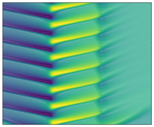
Hostname: page-component-586b7cd67f-r5fsc Total loading time: 0 Render date: 2024-11-22T07:23:40.113Z Has data issue: false hasContentIssue false

Comparative analysis of machine learning methods for active flow control

Published online by Cambridge University Press:  10 March 2023

Fabio Pino*
Affiliation:
EA Department, von Kármán Institute for Fluid Dynamics, 1640 Sint Genesius Rode, Belgium Transfers, Interfaces and Processes (TIPs), Université libre de Bruxelles, 1050 Brussels, Belgium
Lorenzo Schena
Affiliation:
EA Department, von Kármán Institute for Fluid Dynamics, 1640 Sint Genesius Rode, Belgium Department of Mechanical Engineering, Vrije Universiteit Brussels, 1050 Brussels, Belgium
Jean Rabault
Affiliation:
Norwegian Meteorological Institute, 0313 Oslo, Norway
Miguel A. Mendez
Affiliation:
EA Department, von Kármán Institute for Fluid Dynamics, 1640 Sint Genesius Rode, Belgium
*
Email address for correspondence: fabio.pino@vki.ac.be

Abstract

Machine learning frameworks such as genetic programming and reinforcement learning (RL) are gaining popularity in flow control. This work presents a comparative analysis of the two, benchmarking some of their most representative algorithms against global optimization techniques such as Bayesian optimization and Lipschitz global optimization. First, we review the general framework of the model-free control problem, bringing together all methods as black-box optimization problems. Then, we test the control algorithms on three test cases. These are (1) the stabilization of a nonlinear dynamical system featuring frequency cross-talk, (2) the wave cancellation from a Burgers’ flow and (3) the drag reduction in a cylinder wake flow. We present a comprehensive comparison to illustrate their differences in exploration versus exploitation and their balance between ‘model capacity’ in the control law definition versus ‘required complexity’. Indeed, we discovered that previous RL control attempts of controlling the cylinder wake were performing linear control and that the wide observation space was limiting their performances. We believe that such a comparison paves the way towards the hybridization of the various methods, and we offer some perspective on their future development in the literature of flow control problems.

Type
JFM Papers
Copyright
© The Author(s), 2023. Published by Cambridge University Press

1. Introduction

The multidisciplinary nature of active flow control has attracted interests from many research areas for a long time, (Gad-el Hak Reference Gad-el Hak2000; Bewley Reference Bewley2001; Gunzburger Reference Gunzburger2002; Wang & Feng Reference Wang and Feng2018) and its scientific and technological relevance have ever-growing proportions (Bewley Reference Bewley2001; Brunton & Noack Reference Brunton and Noack2015; Noack, Cornejo Maceda & Lusseyran Reference Noack, Cornejo Maceda and Lusseyran2023). Indeed, the ability to interact and manipulate a fluid system to improve its engineering benefits is essential in countless problems and applications, including laminar to turbulent transition (Schlichting & Kestin Reference Schlichting and Kestin1961; Lin Reference Lin2002), drag reduction (Gad-el Hak Reference Gad-el Hak2000; Wang & Feng Reference Wang and Feng2018), stability of combustion systems (Lang, Poinsot & Candel Reference Lang, Poinsot and Candel1987), flight mechanics (Longuski, Guzmán & Prussing Reference Longuski, Guzmán and Prussing2014), wind energy (Munters & Meyers Reference Munters and Meyers2018; Apata & Oyedokun Reference Apata and Oyedokun2020) and aeroacoustic noise control (Collis, Ghayour & Heinkenschloss Reference Collis, Ghayour and Heinkenschloss2002; Kim, Bodony & Freund Reference Kim, Bodony and Freund2014), to name just a few.

The continuous development of computational and experimental tools, together with the advent of data-driven methods from the ongoing machine learning revolution, is reshaping tools and methods in the field (Noack Reference Noack2019; Noack et al. Reference Noack, Cornejo Maceda and Lusseyran2023). Nevertheless, the quest for reconciling terminology and methods from the machine learning and the control theory community has a long history (see Sutton, Barton & Williams Reference Sutton, Barton and Williams1992; Bersini & Gorrini Reference Bersini and Gorrini1996) and it is still ongoing, as described in the recent review by Recht (Reference Recht2019) and Nian, Liu & Huang (Reference Nian, Liu and Huang2020). This article aims at reviewing some recent machine learning algorithms for flow control, presenting a unified framework that highlights differences and similarities amidst various techniques. We hope that such a generalization opens the path to hybrid approaches.

In its most abstract formulation, the (flow) control problem is essentially a functional optimization problem constrained by the (fluid) systems’ dynamics (Stengel Reference Stengel1994; Kirk Reference Kirk2004). As further discussed in § 2, the goal is to find a control function that minimizes (or maximizes) a cost (or reward) functional that measures the controller performances (e.g. drag or noise reduction). Following Wiener's metaphors (Wiener Reference Wiener1948), active control methods can be classified as white, grey or black depending on how much knowledge about the system is used to solve the optimization: the whiter the approach, the more the control relies on the analytical description of the system to be controlled.

Machine-learning-based approaches are ‘black-box’ or ‘model-free’ methods. These approaches rely only on input–output data, and knowledge of the system is gathered by interacting with it. Bypassing the need for a model (and underlying simplifications), these methods are promising tools for solving problems that are not amenable to analytical treatment or cannot be accurately reproduced in a numerical environment. Machine learning (Mitchell Reference Mitchell1997; Vladimir Cherkassky Reference Vladimir Cherkassky2008; Abu-Mostafa, Magdon-Ismail & Lin Reference Abu-Mostafa, Magdon-Ismail and Lin2012; Brunton, Noack & Koumoutsakos Reference Brunton, Noack and Koumoutsakos2020) is a subset of artificial intelligence that combines optimization and statistics to ‘learn’ (i.e. calibrate) models from data (i.e. experience). These models can be general enough to describe any (nonlinear) function without requiring prior knowledge and can be encoded in various forms: examples are parametric models such as radial basis functions (RBFs, see Fasshauer Reference Fasshauer2007) expansions or artificial neural networks (ANNs, see Goodfellow, Bengio & Courville Reference Goodfellow, Bengio and Courville2016), or tree structures of analytic expressions such as in genetic programming (GP, developed by Koza Reference Koza1994). The process by which these models are ‘fitted’ to (or ‘learned’ from) data is an optimization in one of its many forms (Sun et al. Reference Sun, Cao, Zhu and Zhao2019): continuous or discrete, global or local, stochastic or deterministic. Within the flow control literature, at the time of writing, the two most prominent model-free control techniques from the machine learning literature are GP and reinforcement learning (RL) (Sutton & Barto Reference Sutton and Barto2018). Both are reviewed in this article.

Genetic programming is an evolutionary computational technique developed as a new paradigm for automatic programming and machine learning (Banzhaf et al. Reference Banzhaf, Nordin, Keller and Francone1997; Vanneschi & Poli Reference Vanneschi and Poli2012). Genetic programming optimizes both the structure and parameters of a model, which is usually constructed as recursive trees of predefined functions connected through mathematical operations. The use of GP for flow control has been pioneered and popularized by Noack and coworkers (Duriez, Brunton & Noack Reference Duriez, Brunton and Noack2017; Noack Reference Noack2019). Successful examples on experimental problems include the drag reduction past bluff bodies (Li et al. Reference Li, Noack, Cordier, Borée and Harambat2017), shear flow separation control (Gautier et al. Reference Gautier, Aider, Duriez, Noack, Segond and Abel2015; Benard et al. Reference Benard, Pons-Prats, Periaux, Bugeda, Braud, Bonnet and Moreau2016; Debien et al. Reference Debien, von Krbek, Mazellier, Duriez, Cordier, Noack, Abel and Kourta2016) and many more, as reviewed by Noack (Reference Noack2019). More recent extensions of this ‘machine learning control’ (MLC) approach, combining genetic algorithms with the downhill simplex method, have been proposed by Li et al. (Reference Li, Cui, Jia, Li, Yang, Morzyński and Noack2022) and Cornejo Maceda et al. (Reference Cornejo Maceda, Li, Lusseyran, Morzyński and Noack2021).

Reinforcement learning is one of the three machine learning paradigms and encompasses learning algorithms collecting data ‘online’, in a trial and error process. In deep reinforcement learning (DRL), ANNs are used to parametrize the control law or to build a surrogate of the $Q$ function, defining the value of an action at a given state. The use of an ANN to parametrize control laws has a long history (see Lee et al. Reference Lee, Kim, Babcock and Goodman1997), but their application to flow control, leveraging on RL algorithms, is in its infancy (see also Li & Zhang Reference Li and Zhang2021 for a recent review). The landscape of RL is vast and grows at a remarkable pace, fostered by the recent success in strategy board games (Silver et al. Reference Silver2016Reference Silver2018), video games (Szita Reference Szita2012), robotics (Kober & Peters Reference Kober and Peters2014), language processing (Luketina et al. Reference Luketina, Nardelli, Farquhar, Foerster, Andreas, Grefenstette, Whiteson and Rocktäschel2019) and more. In the literature of flow control, RL has been pioneered by Komoutsakos and coworkers (Gazzola, Hejazialhosseini & Koumoutsakos Reference Gazzola, Hejazialhosseini and Koumoutsakos2014; Verma, Novati & Koumoutsakos Reference Verma, Novati and Koumoutsakos2018); see also Garnier et al. Reference Garnier, Viquerat, Rabault, Larcher, Kuhnle and Hachem2021; Rabault & Kuhnle Reference Rabault and Kuhnle2022 for more literature. The first applications of RL in fluid mechanics were focused on the study of the collective behaviour of swimmers (Novati et al. Reference Novati, Verma, Alexeev, Rossinelli, van Rees and Koumoutsakos2017; Verma et al. Reference Verma, Novati and Koumoutsakos2018; Wang & Feng Reference Wang and Feng2018; Novati & Koumoutsakos Reference Novati and Koumoutsakos2019; Novati, Mahadevan & Koumoutsakos Reference Novati, Mahadevan and Koumoutsakos2019), while the first applications for flow control were presented by Pivot, Cordier & Mathelin (Reference Pivot, Cordier and Mathelin2017), Guéniat, Mathelin & Hussaini (Reference Guéniat, Mathelin and Hussaini2016) and by Rabault et al. (Reference Rabault, Kuchta, Jensen, Réglade and Cerardi2019Reference Rabault, Ren, Zhang, Tang and Xu2020) and Rabault & Kuhnle (Reference Rabault and Kuhnle2019). A similar flow control problem has been solved numerically and experimentally via RL by Fan et al. (Reference Fan, Yang, Wang, Triantafyllou and Karniadakis2020). Bucci et al. (Reference Bucci, Semeraro, Allauzen, Wisniewski, Cordier and Mathelin2019) showcased the use of RL to control chaotic systems such as the one-dimensional (1-D) Kuramoto–Sivashinsky equation; Beintema et al. (Reference Beintema, Corbetta, Biferale and Toschi2020) used it to control heat transport in a two-dimensional (2-D) Rayleigh–Bénard system while Belus et al. (Reference Belus, Rabault, Viquerat, Che, Hachem and Reglade2019) used RL to control the interface of unsteady liquid films. Ongoing efforts in the use of DRL for flow control are focused with increasing the complexity of the analysed test cases, either by increasing the Reynolds number in academic test cases (see Ren, Rabault & Tang Reference Ren, Rabault and Tang2021) or by considering realistic configurations (Vinuesa et al. Reference Vinuesa, Lehmkuhl, Lozano-Durán and Rabault2022).

In this article we consider the deep deterministic policy gradient (DDPG, Lillicrap et al. Reference Lillicrap, Hunt, Pritzel, Heess, Erez, Tassa, Silver and Wierstra2015) as a representative deterministic RL algorithm. This is introduced in § 3.3, and the results obtained for one of the investigated test cases are compared with those obtained by Tang et al. (Reference Tang, Rabault, Kuhnle, Wang and Wang2020) using a stochastic RL approach, namely the proximal policy optimization (PPO) Schulman et al. (Reference Schulman, Wolski, Dhariwal, Radford and Klimov2017).

This work puts GP and RL in a global control framework and benchmarks their performances against simpler black-box optimization methods. Within this category, we include model-free control methods in which the control action is predefined and prescribed by a few parameters (e.g. a simple linear controller), and the model learning is driven by global black-box optimization. This approach, using genetic algorithms, has a long history (Fleming & Fonseca Reference Fleming and Fonseca1993). However, here we focus on more sample efficient alternatives such as the Bayesian optimization (BO) and the Lipschitz global optimization (LIPO) technique. Both are described in § 3.1.

The BO is arguably the most popular ‘surrogate-based’, derivative-free, global optimization tool, popularized by Jones, Schonlau & Welch (Reference Jones, Schonlau and Welch1998) and their efficient global optimization algorithm. In its most classic form (Forrester, Sóbester & Keane Reference Forrester, Sóbester and Keane2008; Archetti & Candelieri Reference Archetti and Candelieri2019), the BO uses a Gaussian process (GPr) (Rasmussen & Williams Reference Rasmussen and Williams2005) for regression of the cost function under evaluation and an acquisition function to decide where to sample next. This method has been used by Mahfoze et al. (Reference Mahfoze, Moody, Wynn, Whalley and Laizet2019) for reducing the skin-friction drag in a turbulent boundary layer and by Blanchard et al. (Reference Blanchard, Cornejo Maceda, Fan, Li, Zhou, Noack and Sapsis2022) for reducing the drag in the fluidic pinball and for enhancing mixing in a turbulent jet.

The LIPO algorithm is a more recent global optimization strategy proposed by Malherbe & Vayatis (Reference Malherbe and Vayatis2017). This is a sequential procedure to optimize a function under the only assumption that it has a finite Lipschitz constant. Since this method has virtually no hyperparameters involved, variants of the LIPO are becoming increasingly popular in hyperparameter calibration of machine learning algorithms (Ahmed, Vaswani & Schmidt Reference Ahmed, Vaswani and Schmidt2020), but to the authors’ knowledge it has never been tested on flow control applications.

All the aforementioned algorithms are analysed on three test cases of different dimensions and complexity. The first test case is the zero-dimensional (0-D) model proposed by Duriez et al. (Reference Duriez, Brunton and Noack2017) as the simplest dynamical system reproducing the frequency cross-talk encountered in many turbulent flows. The second test case is the control of nonlinear travelling waves described by the 1-D Burgers’ equation. This test case is representative of the challenges involved in the control of advection–diffusion problems. Moreover, recent works on Koopman analysis by Page & Kerswell (Reference Page and Kerswell2018) and Balabane, Mendez & Najem (Reference Balabane, Mendez and Najem2021) have provided a complete analytical linear decomposition of the Burgers’ flow and might render this test case more accessible to ‘white-box’ control methods. Finally, the last selected test case is arguably the most well-known benchmark in flow control: the drag attenuation in the flow past a cylinder. This problem has been tackled by nearly the full spectra of control methods in the literature, including reduced-order models and linear control (Park, Ladd & Hendricks Reference Park, Ladd and Hendricks1994; Bergmann, Cordier & Brancher Reference Bergmann, Cordier and Brancher2005; Seidel et al. Reference Seidel, Siegel, Fagley, Cohen and McLaughlin2008), resolvent-based feedback control (Jin, Illingworth & Sandberg Reference Jin, Illingworth and Sandberg2020), RL via stochastic (Rabault et al. Reference Rabault, Kuchta, Jensen, Réglade and Cerardi2019) and deterministic algorithms (Fan et al. Reference Fan, Yang, Wang, Triantafyllou and Karniadakis2020), RL assisted by stability analysis (Li & Zhang Reference Li and Zhang2021) and recently also GP (Castellanos et al. Reference Castellanos, Cornejo Maceda, de la Fuente, Noack, Ianiro and Discetti2022).

We here benchmark both methods on the same test cases against classic black-box optimization. Emphasis is given to the different precautions these algorithms require, the number of necessary interactions with the environment, the different approaches to balance exploration and exploitation, and the differences (or similarities) in the derived control laws. The remainder of the article is structured as follows. Section 2 recalls the conceptual transition from optimal control theory to MLC. Section 3 briefly recalls the machine learning algorithm analysed in this work, while § 4 describes the introduced test cases. Results are collected in § 5 while conclusions and outlooks are given in § 6.

2. From optimal control to machine learning

An optimal control problem consists in finding a control action $\boldsymbol {a}(t)\in \mathcal {A}$, within a feasible set $\mathcal {A}\subseteq {{R}^{n_a}}$, which optimizes a functional measuring our ability to keep a plant in control theory and an environment in RL close to the desired states or conditions. The functional is usually a cost to minimize in control theory and a payoff to maximize in RL. We follow the second and denote the reward function as $R(\boldsymbol {a})$. The optimization is constrained by the plant/environment's dynamic,

(2.1)\begin{equation} \left. \begin{aligned} \max_{\boldsymbol{a}(t)\in\mathcal{A}} & \quad R(\boldsymbol{a})=\phi(\boldsymbol{s}(T)) + \int_{0}^{T} \mathcal{L}(\boldsymbol{s}(\tau),\boldsymbol{a}(\tau),\tau)\, {\rm d}\tau,\\ \text{s.t.} & \quad \begin{cases} \dot{\boldsymbol{s}}(t) = \boldsymbol{f}(\boldsymbol{s}(t),\boldsymbol{a}(t),t), \quad t\in(0,T],\\ \boldsymbol{s}(0)= \boldsymbol{s}_0, \end{cases} \end{aligned} \right\} \end{equation}

where $\boldsymbol {f}:\mathbb {R}^{n_s}\times \mathbb {R}^{n_a}\rightarrow \mathbb {R}^{n_s}$ is the vector field in the phase space of the dynamical system and $\boldsymbol {s}\in \mathbb {R}^{n_s}$ is the system's state vector. The action is taken by a controller in optimal control and an agent in RL.

The functional $R(\boldsymbol {a})$ comprises a running cost (or Lagrangian) $\mathcal {L}:\mathbb {R}^{n_{s}}\times \mathbb {R}^{n_{a}}\rightarrow \mathbb {R}$, which accounts for the system's states evolution, and a terminal cost (or Mayer term) $\phi :\mathbb {R}^{n_s}\rightarrow \mathbb {R}$, which depends on the final state condition. Optimal control problems with this cost functional form are known as the Bolza problem (Evans Reference Evans1983; Stengel Reference Stengel1994; Kirk Reference Kirk2004).

In closed-loop control, the agent/controller selects the action/actuation from a feedback control law or policy ${\rm \pi} : \mathbb {R}^{n_s}\rightarrow \mathbb {R}^{n_a}$ of the kind $\boldsymbol {a}(t)={\rm \pi} (\boldsymbol {s}(t)) \in \mathbb {R}^{n_a}\,$ whereas in open-loop control the action/actuation is independent from the system states, i.e. $\boldsymbol {a}(t)={\rm \pi} (t) \in \mathbb {R}^{n_a}$. One could opt for a combination of the two and consider a control law/policy ${\rm \pi} : \mathbb {R}^{n_s+1}\rightarrow \mathbb {R}^{n_a}$ of the kind $\boldsymbol {a}(t)={\rm \pi} (\boldsymbol {s}(t),t) \in \mathbb {R}^{n_a}$.

All model-free methods seek to convert the variational problem in (2.1) into an optimization problem using function approximators such as tables or parametric models. Some authors treated the machines learning control as a regression problem (Duriez et al. Reference Duriez, Brunton and Noack2017) and others as a dynamic programming problem (Bucci et al. Reference Bucci, Semeraro, Allauzen, Wisniewski, Cordier and Mathelin2019). We here consider the more general framework of black-box optimization, which can be tackled with a direct or indirect approach (see figure 1).

Figure 1. General setting for a machine-learning-based control problem: the learning algorithm (optimizer) improves the agent/control performances while this interacts with the environment/plant. Here $k$ spans the number of interactions within an episode and $n$ spans the number of episodes during the training. A function approximator is used for the actuation policy in (a) and the state-value function in (b). In both cases, the control problem is an optimization problem for the parameters $\boldsymbol {w}$.

In the black-box optimization setting, the function to optimize is unknown and the optimization relies on the sampling of the cost function. Likewise, the equations governing the environment/plant are unknown in model-free control techniques and the controller design solely relies on trial and error. We define the discrete version of (2.1) by considering a uniform time discretization $t_k=k\Delta t$ in the interval $t\in [0,T]$, leading to $N=T/\Delta t+1$ points indexed as $k=0,\ldots N-1$. Introducing the notation $\boldsymbol {s}_k=\boldsymbol {s}(t_k)$, we collect a sequence of states $\boldsymbol {S}:=\{\boldsymbol {s}_1,\boldsymbol {s}_2\ldots \boldsymbol {s}_N\}$ while taking a sequence of actions $\boldsymbol {A}^{{\rm \pi} }:=\{\boldsymbol {a}_1,\boldsymbol {a}_2\ldots \boldsymbol {a}_N\}$. Collecting also the reward $\mathcal {L}(\boldsymbol {s}_k,\boldsymbol {a}_k,k)$, each state-action pair allows for defining the sampled reward as

(2.2)\begin{equation} R(\boldsymbol{A}^{\rm \pi})=\phi(\boldsymbol{s}_N)+\sum^{N-1}_{k=0}\mathcal{L}(\boldsymbol{s}_k,\boldsymbol{a}^{\rm \pi}_k,k), \end{equation}

where $N$ is the number of interactions with the systems and defines the length of an episode, within which performances are evaluated. In the RL literature, this is known as cumulative reward and the Lagrangian takes the form $\mathcal {L}(\boldsymbol {s}_k,\boldsymbol {a}^{{\rm \pi} }_k,k)=\gamma ^{k} r(\boldsymbol {s}_k,\boldsymbol {a}^{{\rm \pi} }_k)=\gamma ^{k} r^{{\rm \pi} }_k$, where $\gamma \in [0,1]$ is a discount factor to prioritize immediate over future rewards.

The direct approach (figure 1a) consists in learning an approximation of the optimal policy from the data collected. In the RL literature these methods are referred to as ‘on policy’ if the samples are collected following the control policy and ‘off policy’ if these are collected following a behavioural policy that might significantly differ from the control policy.

Focusing on deterministic policies, the function approximation can take the form of a parametric function $\boldsymbol {a}^{\rm \pi} ={\rm \pi} (\boldsymbol {s};\boldsymbol {w})$, where $\boldsymbol {w}\in \mathbb {R}^{n_w}$ is the set of (unknown) weights that must be learned. On the other hand, in a stochastic policy the parametric function outputs the parameters of the distribution (e.g. mean and standard deviation in a Gaussian) from which the actions will be sampled. In either case, the cumulative reward is now a function of the weights controlling the policy and the learning is the iterative process that leads to larger $R(\boldsymbol {w}_n)$ episode after episode (cf. figure 1a). The update of the weights can be carried out at each interaction $k$ or at each episode $n$. Moreover, one might simultaneously train multiple versions of the same parametrization (i.e. advance multiple candidates at the same time) and seek to improve the policy by learning from the experience of all candidates. In multi-agent RL the various agents (candidates) could cooperate or compete (Buşoniu, Babuška & Schutter Reference Buşoniu, Babuška and Schutter2010; Lowe et al. Reference Lowe, Wu, Tamar, Harb, Abbeel and Mordatch2017).

In the classic GP approach to model-free control (Duriez et al. Reference Duriez, Brunton and Noack2017), the function approximation is built via expression trees and $\boldsymbol {w}$ is a collection of strings that define the operations in the tree. The GP trains a population of agents, selecting the best candidates following an evolutionary approach. Concerning the BO and LIPO implemented in this work and described in the following section, it is instructive to interpret these as single-agent and ‘on-policy’ RL approaches, with policy embedded in a parametric function and training governed by a surrogate-based optimizer that updates the parameters at the end of each episode.

In contrast to direct methods, indirect methods (figure 1b) do not use function approximators for the policy but seek to learn an estimation of the state-value function $Q$, also known as the $Q$ function in RL. For a deterministic agent/controller and deterministic environment/plant, this is defined as

(2.3)\begin{equation} \boldsymbol{Q}^{\rm \pi}(\boldsymbol{s}_t,{\boldsymbol{a}}_t)= \phi_r(\boldsymbol{s}_N)+r(\boldsymbol{s}_t,{\boldsymbol{a}}_t) +\sum^N_{k=t+1}\mathcal{L}_r(\boldsymbol{s}_k,\boldsymbol{a}^{\rm \pi}_k,k) =r(\boldsymbol{s}_t,{\boldsymbol{a}}_t)+\gamma \boldsymbol{V}^{\rm \pi}(\boldsymbol{s}_{t+1}), \end{equation}

where

(2.4)\begin{equation} \boldsymbol{V}^{\rm \pi}(\boldsymbol{s}_t)= \phi(\boldsymbol{s}_N)+\sum^N_{k=t}\mathcal{L}_r(\boldsymbol{s}_k,\boldsymbol{a}^{\rm \pi}_k,k)= \phi(\boldsymbol{s}_N)+\sum^N_{k=t}\gamma^{k-t} r^{\rm \pi}_k =r_k+\gamma \boldsymbol{V}^{\rm \pi}(\boldsymbol{s}_{t+1}) \end{equation}

is the value function according to policy ${\rm \pi}$, i.e. the cumulative reward one can get starting from state $\boldsymbol {s}_t$ and then following the policy ${\rm \pi}$. The $Q$ function gives the value of an action at a given state; if a good approximation of this function is known, the best action is simply the greedy $\boldsymbol {a}_k=\operatorname {arg\,max}_{a_k} Q(\boldsymbol {s}_t,\boldsymbol {a}_t)$. Then, if $Q(\boldsymbol {s}_k,\boldsymbol {a}_k;\boldsymbol {w}_n)$ denotes the parametric function approximating $Q(\boldsymbol {s}_k,\boldsymbol {a}_k)$, learning is the iterative process by which the approximation improves, getting closer to the definition in (2.3). The black-box optimization perspective is thus the minimization of the error in the $Q$ prediction; this could be done with a huge variety of tools from optimization.

Methods based on the $Q$ function are ‘off policy’ and descend from dynamic programming (Sutton & Barto Reference Sutton and Barto2018). The most classic approach is deep $Q$ learning (DQN, Mnih et al. Reference Mnih, Kavukcuoglu, Silver, Graves, Antonoglou, Wierstra and Riedmiller2013). ‘Off-policy’ methods are rather uncommon in the literature of flow control and are now appearing with the diffusion of RL approaches. While most authors use ANNs as function approximators for the $Q$ function, alternatives have been explored in other fields. For example, Kubalik et al. (Reference Kubalik, Derner, Zegklitz and Babuska2021) uses a variant of GP while Kuss & Rasmussen (Reference Kuss and Rasmussen2003), Goumiri, Priest & Schneider (Reference Goumiri, Priest and Schneider2020) and Fan, Chen & Wang (Reference Fan, Chen and Wang2018) use Gaussian processes as in classic BO. We also remark that the assumption of a deterministic system is uncommon in the literature of RL, where the environment is usually treated as a Markov decision process (MDP). We briefly reconsider the stochastic approach in the description of the DDPG in § 3.3. Like many modern RL algorithms, the DDPG implemented in this work combines both ‘on-policy’ and ‘off-policy’ approaches.

3. Implemented algorithms

3.1. Optimization via BO and LIPO

We assume that the policy is a predefined parametric function $\boldsymbol {a}={\rm \pi} (\boldsymbol {s}_t;\boldsymbol {w}^{{\rm \pi} })\in \mathbb {R}^{n_a}$ with a small number of parameters (say $n_w \sim {O}(10)$). The dimensionality of the problem enables efficient optimizers such as BO and LIPO; other methods are illustrated by Duriez et al. (Reference Duriez, Brunton and Noack2017).

3.1.1. Bayesian optimization

The classic BO uses a GPr as surrogate model of the function that must be optimized. In the ‘on-policy’ approach implemented in this work, this is the cumulative reward function $R(\boldsymbol {w})$; from (2.3) and (2.4), this is $R(\boldsymbol {w})=V^{{\rm \pi} }(\boldsymbol {s}_0)=Q(\boldsymbol {s_0},\boldsymbol {a}^{{\rm \pi} }_0)$.

Let $\boldsymbol {W}^*:=\{\boldsymbol {w}_1,\boldsymbol {w}_2\ldots \boldsymbol {w}_{n_*}\}$ be a set of $n_*$ tested weights and $\boldsymbol {R}^*:=\{R_1,R_2\ldots {R}_{n_*}\}$ the associated cumulative rewards. The GPr offers a probabilistic model that computes the probability of a certain reward given the observations $(\boldsymbol {W}^*,\boldsymbol {R}^*)$, i.e. $p(R(\boldsymbol {w})|\boldsymbol {W}^*,\boldsymbol {R}^{*})$. In a GPr this is

(3.1)\begin{equation} p(R(\boldsymbol{w})|\boldsymbol{R}^*,\boldsymbol{W}^*)= \mathcal{N}(\boldsymbol{\mu},\boldsymbol{\varSigma}), \end{equation}

where $\mathcal {N}$ denotes a multivariate Gaussian distribution with mean $\boldsymbol {\mu }$ and covariance matrix $\boldsymbol {\varSigma }$. In a Bayesian framework, (3.1) is interpreted as a posterior distribution, conditioned to the observations ($\boldsymbol {W}^*,\boldsymbol {R}^*$). A GPr is a distribution over functions whose smoothness is defined by the covariance function, computed using a kernel function. Given a set of data $(\boldsymbol {W}^*,\boldsymbol {R}^*)$, this allows for building a continuous function to estimate both the reward of a possible candidate and the uncertainties associated with it.

We are interested in evaluating (3.1) on a set of $n_E$ new samples $\boldsymbol {W}:=\{\boldsymbol {w}_1,\boldsymbol {w}_2\ldots \boldsymbol {w}_{n_E}\}$ and we denote as $\boldsymbol {R}:=\{R_1,R_2\ldots R_{n_E}\}$ the possible outcomes (treated as random variables). Assuming that the possible candidate solutions belong to the same GPr (usually assumed to have zero mean (Rasmussen & Williams Reference Rasmussen and Williams2005)) as the observed data $(\boldsymbol {W}^*,\boldsymbol {R}^*)$, we have

(3.2)\begin{equation} \begin{pmatrix}\boldsymbol{R}^* \\ \boldsymbol{R}\end{pmatrix} \sim \mathcal{N} \left(\boldsymbol{0}, \begin{pmatrix}\boldsymbol{K}_{**} & \boldsymbol{K}_* \\ \boldsymbol{K}_*^T & \boldsymbol{K}\end{pmatrix} \right), \end{equation}

where $\boldsymbol {K}_{**}=\kappa (\boldsymbol {W}^*,\boldsymbol {W}^*) \in \mathbb {R}^{n_*\times n_*}$, $\boldsymbol {K}_{*}=\kappa (\boldsymbol {W},\boldsymbol {W}^*)\in \mathbb {R}^{n_E\times n_*}$, $\boldsymbol {K}=\kappa (\boldsymbol {W},\boldsymbol {W})\in \mathbb {R}^{n_E\times n_E}$ and $\kappa$ a kernel function.

The prediction in (3.1) can be built using standard rules for conditioning multivariate Gaussian, and the functions $\boldsymbol {\mu }$ and $\boldsymbol {\varSigma }$ in (3.1) become a vector $\boldsymbol {\mu _*}$ and a matrix $\boldsymbol {\varSigma _*}$,

(3.3)$$\begin{gather} \boldsymbol{\mu_*} = \boldsymbol{K}_*^T \boldsymbol{K}_R^{{-}1} \boldsymbol{R}^*\quad\in \mathbb{R}^{n_E}, \end{gather}$$
(3.4)$$\begin{gather}\boldsymbol{\varSigma_*} = \boldsymbol{K} - \boldsymbol{K}_*^T \boldsymbol{K}_R^{{-}1} \boldsymbol{K}_*\quad\in \mathbb{R}^{n_E\times n_E}, \end{gather}$$

where $\boldsymbol {K}_R=\boldsymbol {K}_{**}+\sigma _{R}^2\boldsymbol {I}$, with $\sigma _{R}^2$ the expected variance in the sampled data and $\boldsymbol {I}$ the identity matrix of appropriate size. The main advantage of BO is that the function approximation is sequential, and new predictions improve the approximation of the reward function (i.e. the surrogate model) episode after episode. This makes the GPr-based BO one of the most popular black-box optimization methods for expensive cost functions.

The BO combines the GPr model with a function suggesting where to sample next. Many variants exist (Frazier Reference Frazier2018), each providing their exploration/exploitation balance. The exploration seeks to sample in regions of large uncertainty, while exploitation seeks to sample at the best location according to the current function approximation. The most classic function, used in this study, is the expected improvement, defined as (Rasmussen & Williams Reference Rasmussen and Williams2005)

(3.5)\begin{equation} \operatorname{EI}(\boldsymbol{w}) = \begin{cases} (\varDelta - \xi)\varPhi(Z) + \sigma(\boldsymbol{w})\phi(Z) & \text{if}\ \sigma(\boldsymbol{w}) > 0,\\ 0 & \text{if}\ \sigma(\boldsymbol{w}) = 0, \end{cases} \end{equation}

with $\varDelta =\mu (\boldsymbol {w}) - R(\boldsymbol {w}^+)$ and $\boldsymbol {w}^+=\operatorname {arg\,max}_{\boldsymbol {w}} \tilde {R}(\boldsymbol {w})$ the best sample so far, where $\varPhi (Z)$ is the cumulative distribution function, $\phi (Z)$ is the probability density function of a standard Gaussian and

(3.6)\begin{equation} Z = \begin{cases} \dfrac{\varDelta- \xi}{\sigma(\boldsymbol{w})} & \text{if}\ \sigma(\boldsymbol{w}) > 0 ,\\ 0 & \text{if}\ \sigma(\boldsymbol{w}) = 0. \end{cases} \end{equation}

Equation (3.5) balances the desire to sample in regions where $\mu (\boldsymbol {w})$ is larger than $R(\boldsymbol {w}^+)$ (hence, large and positive $\varDelta$) versus sampling in regions where $\sigma (\boldsymbol {w})$ is large. The parameter $\xi$ sets a threshold over the minimal expected improvement that justifies the exploration.

Finally, the method requires the definition of the kernel function and its hyperparameters, as well as an estimate of $\sigma _y$. In this work the GPr-based BO was implemented using the Python API scikit-optimize (Head et al. Reference Head, Kumar, Nahrstaedt, Louppe and Shcherbatyi2020). The selected kernel function was a Mater kernel with $\nu =5/2$ (see Chapter 4 from Rasmussen & Williams Reference Rasmussen and Williams2005), which reads

(3.7)\begin{equation} \kappa (\boldsymbol{x},\boldsymbol{x}')=\kappa (r)=1+\frac{\sqrt{5} r}{l}+\frac{5 r^2}{3 l^2}\exp-\frac{\sqrt{5} r}{l}, \end{equation}

where $r=\|\boldsymbol {x}-\boldsymbol {x}'\|_2$ and $l$ is the length scale of the process. We report a detailed description of the pseudocode we used in Appendix A.1.

3.1.2. Lipschitz global optimization

Like BO, LIPO relies on a surrogate model to select the next sampling points (Malherbe & Vayatis Reference Malherbe and Vayatis2017). However, LIPO's surrogate function is the much simpler upper bound approximation $U(\boldsymbol {w})$ of the cost function $R(\boldsymbol {w})$ (Ahmed et al. Reference Ahmed, Vaswani and Schmidt2020). In the dlib implementation by King (Reference King2009), used in this work, this is given by

(3.8)\begin{equation} U(\boldsymbol{w})= \min_{i=1\ldots t}\left(R(\boldsymbol{w}_{i}) + \sqrt{\sigma_i + (\boldsymbol{w}-\boldsymbol{w}_i)^TK(\boldsymbol{w}-\boldsymbol{w}_i)} \right), \end{equation}

where $\boldsymbol {w}_i$ are the sampled parameters, $\sigma _i$ are coefficients that account for discontinuities and stochasticity in the objective function, and $K$ is a diagonal matrix that contains the Lipschitz constants $k_i$ for the different dimensions of the input vector. We recall that a function $R(\boldsymbol {w}):\mathcal {W}\subseteq \mathbb {R}^{n_w}\rightarrow \mathbb {R}$ is a Lipschitz function if there exists a constant $C$ such that

(3.9)\begin{equation} \lVert R(\boldsymbol{w}_1) - R(\boldsymbol{w}_2)\rVert \leq C\lVert\boldsymbol{w}_1 - \boldsymbol{w}_2\rVert, \quad \forall\ \boldsymbol{w}_1,\boldsymbol{w}_2\in\mathcal{W}, \end{equation}

where $\lVert {\cdot }\rVert$ is the Euclidean norm on $\mathbb {R}^{n_w}$. The Lipshitz constant $k$ of $R(\boldsymbol {w})$ is the smallest $C$ that satisfies the above condition (Davidson & Donsig Reference Davidson and Donsig2009). In other terms, this is an estimate of the largest possible slope of the function $R(\boldsymbol {w})$. The values of $K$ and $\boldsymbol {\sigma }_i$ are found by solving the optimization problem

(3.10)\begin{equation} \left. \begin{aligned} \min_{K,\sigma} & \quad \lVert K\rVert_F^{2} + 10^6\sum_{i=1}^{t}\,\sigma_i^2, \\ \text{s.t.} & \quad U(\boldsymbol{w}_i)\geq R(\boldsymbol{w}_i),\quad \forall i\in[1\cdots t], \\ & \quad \sigma_i \geq 0,\quad \forall i\in[1\cdots t], \\ & \quad K_{i,j} \geq 0,\quad \forall i,j\in[1\cdots d], \\ & \quad \text{K} = \{k_1,k_2,\ldots,k_{n_w}\}, \end{aligned} \right\} \end{equation}

where $10^6$ is a penalty factor and $\lVert\ {\cdot }\ \rVert _F$ is the Frobenius norm.

To compensate for the poor convergence of LIPO in the area around local optima, the algorithm alternates between a global and a local search. If the iteration number is even, it selects the new weights by means of the maximum upper bounding position (MaxLIPO),

(3.11)\begin{equation} \boldsymbol{w}_{k+1} = \mathop {{\rm arg}\ {\rm max}}\limits_{\boldsymbol{w}}(U(\boldsymbol{w})), \end{equation}

otherwise, it relies on a trust region (TR) method (Powell Reference Powell2006) based on a quadratic approximation of $R(\boldsymbol {w})$ around the best weights obtained so far $\boldsymbol {w}^*$, i.e.

(3.12) \begin{equation} \left. \begin{gathered} \boldsymbol{w}_{k+1} =\arg\max_{\boldsymbol{w}} \overbrace{(\boldsymbol{w}^* + g(\boldsymbol{w}^*)^{T}\boldsymbol{w} + \tfrac{1}{2}\boldsymbol{w}^T\boldsymbol{H} (\boldsymbol{w}^*)\boldsymbol{w})}^{m(\boldsymbol{w};\boldsymbol{w}^*)}, \\ \text{s.t.} \|\boldsymbol{w}_{k+1}\|< d(\boldsymbol{w}^*), \end{gathered} \right\} \end{equation}

where $g(\boldsymbol {w}^*)$ is the approximation of the gradient at $\boldsymbol {w}^*$ ($g(\boldsymbol {w}^*)\approx \boldsymbol {\nabla } R(\boldsymbol {w}^*))$, $\boldsymbol {H}(\boldsymbol {w}^*)$ is the approximation of the Hessian matrix $(\boldsymbol {H}(\boldsymbol {w}^*))_{ij} \approx {\partial ^2 R(\boldsymbol {w}^*)}/{\partial \boldsymbol {w}_i\partial \boldsymbol {w}_j}$ and $d(\boldsymbol {w}^*)$ is the radius of the trust region. If the TR-method converges to a local optimum with an accuracy smaller than $\epsilon$,

(3.13)\begin{equation} |R(\boldsymbol{w}_{k})-R(\boldsymbol{w}^*)|<\varepsilon, \quad \forall \boldsymbol{w}_{k}, \end{equation}

the optimization goes on with the global search method until it finds a better optimum. A detailed description of the pseudocode we used can be found in Appendix A.2.

3.2. Genetic programming

In the GP approach to optimal control, the policy $\boldsymbol {a}={\rm \pi} (\boldsymbol {s};\boldsymbol {w})$ is encoded in the form of a syntax tree. The parameters are lists of numbers and functions that can include arithmetic operations, mathematical functions, Boolean operations, conditional operations or iterative operations. An example of a syntax tree representation of a function is shown in figure 2. A tree (or program in GP terminology) is composed of a root that branches out into nodes (containing functions or operations) throughout various levels. The number of levels defines the depth of the tree, and the last nodes are called terminals or leaves. These contain the input variables or constants. Any combination of branches below the root is called a subtree and can generate a tree if the node becomes a root.

Figure 2. Syntax tree representation of the function $2 x\sin (x)+\sin (x)+3$. This tree has a root ‘+’ and a depth of two. The nodes are denoted with orange circles while the last entries are leafs.

Syntax trees allow encoding complex functions by growing into large structures. The trees can adapt during the training: the user provides a primitive set, i.e. the pool of allowed functions, the maximum depth of the tree and set the parameters of the training algorithm. Then, the GP operates on a population of possible candidate solutions (individuals) and evolves it over various steps (generations) using genetic operations in the search for the optimal tree. Classic operations include elitism, replication, cross-over and mutations, as in genetic algorithm optimization (Haupt & Ellen Haupt Reference Haupt and Ellen Haupt2004). The implementation of GP in this work was carried out in the distributed evolutionary algorithms in Python (DEAP) (Fortin et al. Reference Fortin, De Rainville, Gardner, Parizeau and Gagné2012) framework. This is an open-source Python library allowing for the implementation of various evolutionary strategies.

We used a primitive set of four elementary operations ($+,-,/,\times$) and four functions ($\exp,\log,\sin,\cos$). In the second test case, as described in § 5.2, we also include an ephemeral random constant. The initial population of individuals varied between $n_I=10$ and $n_I=80$ candidates depending on the test case and the maximum depth tree was set to $17$. In all test cases the population was initialized using the ‘half-half’ approach, whereby half the population is initialized with the full method and the rest with the growth method. In the full method trees are generated with a predefined depth and then filled randomly with nodes and leafs. In the growth method trees are randomly filled from the roots: because nodes filled with variables or constant are terminals, this approach generates trees of variable depth.

Among the optimizers available in DEAP, in this work we used the $(\mu +\lambda )$ algorithm for the first two test cases and eaSimple (Banzhaf et al. Reference Banzhaf, Nordin, Keller and Francone1997; Vanneschi & Poli Reference Vanneschi and Poli2012; Kober & Peters Reference Kober and Peters2014; Bäck, Fogel & Michalewicz Reference Bäck, Fogel and Michalewicz2018) for the third one. These differ in how the population is updated at each iteration. In the $(\mu +\lambda )$ both the offsprings and parents participate to the tournament while in eaSimple no distinction is made between parents and offsprings and the population is entirely replaced at each iteration.

Details about the algorithmic implementation of this approach can be found in Appendix A.3.

3.3. Reinforcement learning via DDPG

The DDPG by Lillicrap et al. (Reference Lillicrap, Hunt, Pritzel, Heess, Erez, Tassa, Silver and Wierstra2015) is an off-policy actor–critic algorithm using an ANN to learn the policy (direct approach, figure 1a) and an ANN to learn the $Q$ function (indirect approach, figure 1b). In what follows, we call the $\varPi$ network the first (i.e. the actor) and the $Q$ network the second (i.e. the critic).

The DDPG combines the DPG by Silver et al. (Reference Silver, Lever, Heess, Degris, Wierstra and Riedmiller2014) and the DQN by Mnih et al. (Reference Mnih, Kavukcuoglu, Silver, Graves, Antonoglou, Wierstra and Riedmiller2013Reference Mnih2015). The algorithm has evolved into more complex versions such as the twin delayed DDPG (Fujimoto, van Hoof & Meger Reference Fujimoto, van Hoof and Meger2018), but in this work we focus on the basic implementation.

The policy encoded in the $\varPi$ network is deterministic and acts according to the set of weights and biases $\boldsymbol {w}^{{\rm \pi} }$, i.e. $\boldsymbol {a}={\rm \pi} (\boldsymbol {s}_t,\boldsymbol {w}^{{\rm \pi} })$. The environment is assumed to be stochastic and modelled as a MDP. Therefore, (2.3) must be modified to introduce an expectation operator,

(3.14)\begin{equation} Q^{\rm \pi}(\boldsymbol{s}_t,\boldsymbol{a}_t)=\mathbb{E}_{\boldsymbol{s}_{t},\boldsymbol{s}_{t+1}\sim E}\left[r(\boldsymbol{s}_t,\boldsymbol{a}_t)+\gamma Q^{\rm \pi}(\boldsymbol{s}_{t+1},\boldsymbol{a}^{\rm \pi}_{t+1})\right], \end{equation}

where the policy is intertwined in the action state relation, i.e. $Q^{{\rm \pi} }(\boldsymbol {s}_{t+1},\boldsymbol {a}_{t+1})=Q^{{\rm \pi} }(\boldsymbol {s}_{t+1},\boldsymbol {a}^{{\rm \pi} }(\boldsymbol {s}_{t+1}))$ and having used the shorthand notation $\boldsymbol {a}^{{\rm \pi} }_{t+1}={\rm \pi} (\boldsymbol {s}_{t+1},\boldsymbol {w}^{{\rm \pi} })$. Because the expectation operator in (3.14) solely depends on the environment ($E$ in the expectation operator), it is possible to decouple the problem of learning the policy ${\rm \pi}$ from the problem of learning the function $Q^{{\rm \pi} }(\boldsymbol {s}_t,\boldsymbol {a}_t)$. Concretely, let $Q(\boldsymbol {s}_t,\boldsymbol {a}_t;\boldsymbol {w}^{Q})$ denote the prediction of the $Q$ function by the $Q$ network, defined with weights and biases $\boldsymbol {w}^{Q}$ and let $\mathcal {T}$ denote a set of $N$ transitions $(\boldsymbol {s}_t,\boldsymbol {a}_t,\boldsymbol {s}_{t+1},r_{t+1})$ collected through (any) policy. The performances of the $Q$ network can be measured as

(3.15) \begin{equation} J^Q(\boldsymbol{w}^{Q})=\mathbb{E}_{\boldsymbol{s}_t,\boldsymbol{a}_t, \boldsymbol{r}_t\sim \mathcal{T}}[(Q(\boldsymbol{s}_t,\boldsymbol{a}_t; \boldsymbol{w}^{Q})-y_t)^2], \end{equation}

where the term in the squared brackets, called temporal difference (TD), is the difference between the old $Q$ value and the new one $y_t$, known as the TD target,

(3.16)\begin{equation} y_t=r(\boldsymbol{s}_t,\boldsymbol{a}_t)+\gamma Q (\boldsymbol{s}_{t+1},\boldsymbol{a}_{t+1};\boldsymbol{w}^{Q}). \end{equation}

Equation (3.15) measures how closely the prediction of the $Q$ network satisfies the discrete Bellman equation (2.3). The training of the $Q$ network can be carried out using standard stochastic gradient descent methods using the back-propagation algorithm (Kelley Reference Kelley1960) to evaluate $\partial _{\boldsymbol {w}^{Q}} J^Q$.

The training of the $Q$ network gives the off-policy flavour to the DDPG because it can be carried out with an exploratory policy that largely differs from the final policy. Nevertheless, because the training of the $Q$ network is notoriously unstable, Mnih et al. (Reference Mnih, Kavukcuoglu, Silver, Graves, Antonoglou, Wierstra and Riedmiller2013Reference Mnih2015) introduced the use of a replay buffer to leverage accumulated experience (previous transitions) and a target network to under-relax the update of the weights during the training. Both the computation of the cost function in (3.15) and its gradient are performed over a random batch of transitions $\mathcal {T}$ in the replay buffer $\mathcal {R}$.

The DDPG combines the $Q$ network prediction with a policy gradient approach to train the $\varPi$ network. This is inherited from the DPG by Silver et al. (Reference Silver, Lever, Heess, Degris, Wierstra and Riedmiller2014), who have shown that, given

(3.17)\begin{equation} J^{\rm \pi}(\boldsymbol{w}^{\rm \pi})=\mathbb{E}_{\boldsymbol{s}_t\sim E,\boldsymbol{a}_t\sim {\rm \pi}}\left[(r(\boldsymbol{s}_t,\boldsymbol{a}_t))\right] \end{equation}

is the expected return from the initial condition, the gradient with respect to the weights in the $\varPi$ network is

(3.18)\begin{equation} \partial_{\boldsymbol{w}^{\rm \pi}}J^{\rm \pi}=\mathbb{E}_{\boldsymbol{s}_t\sim E,\boldsymbol{a}_t\sim {\rm \pi}}[\partial_{\boldsymbol{a}} Q(\boldsymbol{s}_t,\boldsymbol{a}_t;\boldsymbol{w}^Q)\,\partial_{\boldsymbol{w}^{\rm \pi}} \boldsymbol{a}(\boldsymbol{s}_t;\boldsymbol{w}^{\rm \pi})]. \end{equation}

Both $\partial _{\boldsymbol {a}} Q(\boldsymbol {s}_t,\boldsymbol {a}_t; \boldsymbol {w}^Q)$ and $\partial _{\boldsymbol {w}^{{\rm \pi} }} \boldsymbol {a}(\boldsymbol {s}_t;\boldsymbol {w}^{{\rm \pi} })$ can be evaluated via back propagation on the $Q$ network and the $\varPi$ network, respectively. The main extension of DDPG over DPG is the use of DQN for the estimation of the $Q$ function.

In this work we implement the DDPG using Keras API in Python with three minor modifications to the original algorithm. The first is a clear separation between the exploration and exploitation phases. In particular, we introduce a number of exploratory episodes $n_{Ex}< n_{Ep}$ and the action is computed as

(3.19)\begin{equation} \boldsymbol{a}(\boldsymbol{s}_t)=\boldsymbol{a}(\boldsymbol{s}_t;\boldsymbol{w}^{\rm \pi})+\eta(\mbox{ep})\mathcal{E}(t;\theta,\sigma^2), \end{equation}

where $\mathcal {E}(t;\theta,\sigma )$ is an exploratory random process characterized by a mean $\theta$ and variance $\sigma ^2$. This could be the time-correlated (Uhlenbeck & Ornstein Reference Uhlenbeck and Ornstein1930) noise or white noise, depending on the test case at hand (see § 4). The transition from exploration to exploitation is governed by the parameter $\eta$, which is taken as $\eta (\mbox {ep})=1$ if $\mbox {ep}< n_{Ex}$ where $d^{{ep}-n_{Ex}}$ if $\mbox {ep}>n_{Ex}$. This decaying term for $\mbox {ep}>n_{Ep}$ progressively reduces the exploration and the coefficient $d$ controls how rapidly this is done.

The second modification is in the selection of the transitions from the replay buffer $\mathcal {R}$ that are used to compute the gradient $\partial _{\boldsymbol {w}^{Q}} J^Q$. While the original implementation selects these randomly, we implement a simple version of the prioritized experience replay from Schaul et al. (Reference Schaul, Quan, Antonoglou and Silver2015). The idea is to prioritize, while sampling from the replay buffer, those transitions that led to the largest improvement in the network performances. These can be measured in terms of the TD error

(3.20)\begin{equation} \delta = r_t + \gamma Q(\boldsymbol{s}_{t+1}, \boldsymbol{a}^{\rm \pi}_{t+1};\boldsymbol{w}^{Q})- Q(\boldsymbol{s}_t, a_t;\boldsymbol{w}^{Q}). \end{equation}

This quantity measures how much a transition was unexpected. The rewards stored in the replay buffer ($r_{t}^{RB}$) and used in the TD computation are first scaled using a dynamic vector $r_{log}=[r^{RB}_1,r^{RB}_2,\ldots,r^{RB}_t]$ as

(3.21)\begin{equation} r_{t}^{RB} = \frac{r_t - \bar{r}_{log}}{{\rm std}(r_{log})+1\times 10^{{-}10}}, \end{equation}

where $\bar {r}_{log}$ is the mean value and $\textrm {std}(r_{log})$ is the standard deviation. The normalization makes the gradient steeper far from the mean of the sampled rewards, without changing its sign, and is found to speed-up the learning (see also van Hasselt et al. Reference van Hasselt, Guez, Hessel, Mnih and Silver2016).

As discussed by Schaul et al. (Reference Schaul, Quan, Antonoglou and Silver2015), it can be shown that prioritizing unexpected transitions leads to the steepest gradients $\partial _{\boldsymbol {w}^{Q}} J^Q$ and, thus, helps overcome local minima. The sampling is performed following a triangular distribution that assigns the highest probability $p(n)$ to the transition with the largest TD error $\delta$.

The third modification, extensively discussed in previous works on RL for flow control (Rabault & Kuhnle Reference Rabault and Kuhnle2019; Rabault et al. Reference Rabault, Ren, Zhang, Tang and Xu2020; Tang et al. Reference Tang, Rabault, Kuhnle, Wang and Wang2020), is the implementation of a sort of moving average of the actions. In other words, an action is performed for $K$ consecutive interactions with the environment, which in our work occur at every simulation's time step.

We illustrate the neural network architecture employed in this work in figure 3. The scheme in the figure shows how the $\varPi$ network and the $Q$ network are interconnected: intermediate layers map the current state and the action (output by the $\varPi$ network) to the core of the $Q$ network. For plotting purposes, the number of neurons in the figure is much smaller than the one actually used and indicated in the figure. The $\varPi$ network has two hidden layers with $128$ neurons each, while the input and output depends on the test cases considered (see § 4). Similarly, the $Q$ network has two hidden layers with $128$ neurons each and intermediate layers as shown in the figure. During the exploration phase, the presence of the stochastic term in the action selection decouples the two networks.

Figure 3. The ANN architecture of the DDPG implementation analysed in this work. The illustrated architecture is the one used for the test case in § 4.3. During the exploration phase, the two networks are essentially decoupled by the presence of the stochastic term $\mathcal {E}$ that leads to exploration of the action space.

We detail the main steps of the implemented DDPG algorithm in Appendix A.4. It is important to note that, by construction, the weights in this algorithm are updated at each interaction with the system. Hence, $k=n$ and $N=1$ in the terminology of § 2. The notion of an episode remains relevant to control the transition between various phases of the learning process and to provide comparable metrics between the various algorithms.

4. Test cases

4.1. A 0-D frequency cross-talk problem

The first selected test case is a system of nonlinear ordinary differential equations (ODEs) reproducing one of the main features of turbulent flows: the frequency cross-talk. This control problem was proposed and extensively analysed by Duriez et al. (Reference Duriez, Brunton and Noack2017). It essentially consists in stabilizing two coupled oscillators, described by a system of four ODEs, which describe the time evolution of four leading proper orthogonal decomposition modes of the flow past a cylinder. The model is known as the generalized mean field model (Dirk et al. Reference Dirk, Günther, Noack, King and Tadmor2009) and was used to describe the stabilizing effect of low frequency forcing on the wave flow past a bluff body (Pastoor et al. Reference Pastoor, Henning, Noack, King and Tadmor2008; Aleksic et al. Reference Aleksic, Luchtenburg, King, Noack and Pfeifer2010). The set of ODEs in the states $\boldsymbol {s}(t)=[s_1(t),s_2(t),s_3(t),s_4(t)]^\textrm {T}$, where ($s_1,s_2$) and ($s_3,s_4$) are the first and second oscillator, reads

(4.1)\begin{equation} \dot{\boldsymbol{s}} = \boldsymbol{F}(\boldsymbol{s})\boldsymbol{s} + \boldsymbol{A}\boldsymbol{a}, \end{equation}

where $\boldsymbol {a}$ is the forcing vector with a single scalar component interacting with the second oscillator (i.e. $\boldsymbol {a}=[0,0,0,a]^\textrm {T}$) and the matrix $\boldsymbol {F}(\boldsymbol {s})$ and $\boldsymbol {A}$ are given by

(4.2a,b) \begin{align} \boldsymbol{F}(\boldsymbol{s}) = \begin{bmatrix} \sigma(\boldsymbol{s}) & -1 & 0 & 0\\ 1 & \sigma(\boldsymbol{s}) & 0 & 0 & \\ 0 & 0 & -0.1 & -10 \\ 0 & 0 & 10 & -0.1\!\!\!\!\!\!\!\!\end{bmatrix},\quad \boldsymbol{A} = \left[\!\!\begin{array}{llll@{}l@{}} 0 & 0 & 0 & 0\\ 0 & 0 & 0 & 0 & \\ 0 & 0 & 0 & 0 \\ 0 & 0 & 0 & 1\end{array}\right]. \end{align}

The term $\sigma (\boldsymbol {s})$ models the coupling between the two oscillators:

(4.3)\begin{equation} \sigma(\boldsymbol{s}) = 0.1 - E_1 - E_2, \end{equation}

where $E_1$ and $E_2$ are the energy of the first and second oscillator given by

(4.4a,b)\begin{equation} E_1 = s_1^2+s_2^2 \quad E_2 = s_3^2 + s_4^2. \end{equation}

This nonlinear link is the essence of the frequency cross-talk and challenges linear control methods based on linearization of the dynamical system. To excite the second oscillator, the actuation must introduce energy to the second oscillator, as one can reveal from the associated energy equation. This is obtained by multiplying the last two equations of the system by $s_3$ and $s_4$, respectively, and summing them up to obtain

(4.5)\begin{equation} \tfrac{1}{2}\dot{E_2} ={-}0.2E_2 + s_4 u, \end{equation}

where $u\,s_4$ is the production term associated to the actuation.

The initial conditions are set to $\boldsymbol {s}(0)=[0.01,0,0,0]^\textrm {T}$. Without actuation, the system reaches a ‘slow’ limit cycle involving the first oscillator $(s_1,s_2)$, while the second vanishes ($(s_3,s_4)\rightarrow 0$). The evolution of the oscillator $(s_1,s_2)$ with no actuation is shown in figure 4(a); figure 4(b) shows the time evolution of $\sigma$, which vanishes as the system naturally reaches the limit cycle. Regardless of the state of the first oscillator, the second oscillator is essentially a linear second-order system with eigenvalues $\lambda _{1,2}=-0.1\pm 10\mathrm {i}$; hence, a natural frequency $\omega =10\,\textrm {rad}\,\textrm {s}^{-1}$.

Figure 4. Evolution of the oscillator $(s_1,s_2)$ (a) of the variable $\sigma$ (4.3) (b) in the 0-D test case in the absence of actuation ($a=0$). As $\sigma \approx 0$, the system naturally evolves towards a ‘slow’ limit cycle.

The governing equations (4.1) were solved using scipy's package odeint with a time step of $\Delta \,t={\rm \pi} /50$. This time step is smaller than the one by Duriez et al. (Reference Duriez, Brunton and Noack2017) ($\Delta t={\rm \pi} /10$), as we observed this had an impact on the training performances (aliasing in LIPO and BO optimization).

The actuators’ goal is to bring to rest the first oscillator while exiting the second, leveraging on the nonlinear connection between the two and using the least possible actuation. In this respect, the optimal control law, similarly to Duriez et al. (Reference Duriez, Brunton and Noack2017), is the one that minimizes the cost function

(4.6)\begin{equation} \left.\begin{gathered} J = J_a + \gamma J_b = \overline{s_1^2 + s_2^2} + \alpha \overline{a^2}, \\ \text{where} \quad \overline{f(t)} = \frac{1}{40{\rm \pi}}\int_{20{\rm \pi}}^{60{\rm \pi}} f(t')\, {\rm d}t', \end{gathered} \right\} \end{equation}

where $\alpha$, set to $\alpha =10^{-2}$, is a coefficient set to penalize large actuations. Like the original problem in Duriez et al. (Reference Duriez, Brunton and Noack2017), the actions are clipped to the range $a_k\in [-1,1]$.

The time interval of an episode is set to $t\in [20{\rm \pi},60{\rm \pi} ]$; thus, much shorter than that used by Duriez et al. (Reference Duriez, Brunton and Noack2017). This duration was considered sufficient, as it allows the system to reach the limit cycle and to observe approximately $20$ periods of the slow oscillator. To reproduce the same cost function in a RL framework, we rewrite (4.6) as a cumulative reward, replacing the integral mean with the arithmetic average and setting

(4.7)\begin{equation} J = \frac{1}{n_t}\sum_{k=0}^{n_t-1} s^2_{1k}+s^2_{2k}+\alpha a^2_k={-} \sum_ {k=0}^{n_t-1}r_t={-}R, \end{equation}

with $r_t$ the environment's reward at each time step. For the BO and LIPO optimizers, the control law is defined as a quadratic form of the four system's states,

(4.8)\begin{equation} {\rm \pi}(\boldsymbol{s};\boldsymbol{w}) := \boldsymbol{g}_w^T\boldsymbol{s} + \boldsymbol{s}^T\boldsymbol{H}_w\boldsymbol{s}, \end{equation}

with $\boldsymbol {g}_w\in \mathbb {R}^4$ and $\boldsymbol {H}_w\in \mathbb {R}^{4x4}$. The weight vector associated to this policy is thus $\boldsymbol {w}\in \mathbb {R}^{20}$ and it collects all the entries in $\boldsymbol {g}_w$ and $\boldsymbol {H}_w$. For later reference, the labelling of the weights is as follows:

(4.9a,b)\begin{equation} \boldsymbol{g}_{w}= \begin{bmatrix}w_1\\w_2\\w_3\\w_4 \end{bmatrix} \quad \text{and}\quad \boldsymbol{H}_{w}= \begin{bmatrix}w_5 & w_9 & w_{13} & w_{17}\\w_6 & w_{10} & w_{14} & w_{18}\\w_7 & w_{11} & w_{15} & w_{19}\\w_8 & w_{12} & w_{16} & w_{20} \end{bmatrix}. \end{equation}

Both LIPO and BO seek for the optimal weights in the range $[-3,3]$. The BO was set up with a Matern kernel (see (3.7)) with a smoothness parameter $\nu =1.5$, a length scale of $l=0.01$, an acquisition function based on the expected improvement and an exploitation–exploration (see (3.5)) trade-off parameter $\xi =0.1$. Regarding the learning, 100 episodes were taken for BO, LIPO and DDPG. For the GP, the upper limit is set to 1200, considering 20 generations with $\mu =30$ individuals, $\lambda =60$ offsprings and a ($\mu +\lambda$) approach.

The DDPG experiences are collected with an exploration strategy structured into three parts. The first part (until episode 30) is mostly explorative. Here the noise is clipped in the range $[-0.8,0.8]$ with $\eta =1$ (see (3.19)). The second phase (between episodes 30 and 55) is an off-policy exploration phase with a noise signal clipped in the range $[-0.25,0.25]$, with $\eta =0.25$. The third phase (from episode 55 onwards) is completely exploitative (with no noise). As an explorative signal, we used a white noise with a standard deviation of 0.5.

4.2. Control of the viscous Burgers's equation

We consider the Burger's equation because it offers a simple 1-D problem combining nonlinear advection and diffusion. The problem set is

(4.10)\begin{equation} \left. \begin{aligned} \partial_tu + u\partial_xu & = \nu\partial_{xx}u + f(x,t) + c(x,t),\\ u(x,0) & = u_0,\\ \partial_xu(0,t) & = \partial_xu(L,t)=0, \end{aligned} \right\} \end{equation}

where $(x,t)\in (0,L)\times (0,T]$ with $L=20$ and $T=15$ is the episode length, $\nu =0.9$ is the kinematic viscosity and $u_0$ is the initial condition, defined as the developed velocity field at $t=2.4$ starting from $u(x,0)=0$. The term $f(x,t)$ represents the disturbance and the term $c(x,t)$ is the control actuation, which are both Gaussian functions in space, modulated by a time-varying amplitude,

(4.11)$$\begin{gather} f(x,t)=A_f\sin{(2{\rm \pi} f_p t)}\ {\cdot}\ \mathcal{N}(x-x_f,\sigma), \end{gather}$$
(4.12)$$\begin{gather}c(x,t)=a(t)A_c\ {\cdot}\ \mathcal{N}(x- x_c,\sigma), \end{gather}$$

taking $A_f= 100$ and $f_p=0.5$ for the disturbance's amplitude and frequencies and $A_c=300$ being the amplitude of the control and $a(t)\in [-1,1]$ the action provided by the controller. The disturbance and the controller action are centred at $x_f=6.6$ and $x_c=13.2$, respectively, and have $\sigma =0.2$. The uncontrolled system produces a set of nonlinear waves propagating in both directions at approximately constant velocities. The objective of the controller is to neutralize the waves downstream of the control location, i.e. for $x>x_c$, using three observations at $x=8,9,10$. Because the system's characteristic is such that perturbations propagate in both directions, the impact of the controller propagates backwards towards the sensors and risks being retrofitted in the loop.

To analyse how the various agents deal with the retrofitting problem, we consider two scenarios: a ‘fully closed-loop’ approach and a ‘hybrid’ approach, in which agents are allowed to produce a constant action. The constant term allows for avoiding (or at least limiting) the retrofitting problem. For the BO and LIPO controllers, we consider linear laws; hence, the first approach is

(4.13)\begin{equation} a_A(t;\boldsymbol{w})=w_0 \,u(8,t)+w_1\, u(9,t)+w_2\, u(10,t), \end{equation}

while the second is

(4.14)\begin{equation} a_B(t;\boldsymbol{w})=w_0 \,u(8,t)+w_1\, u(9,t)+w_2\, u(10,t)+w_3. \end{equation}

For the GP, we add the possibility of a constant action using an ephemeral constant, which is a function with no argument that returns a random value. Similarly, we refer to ‘A’ and ‘B’ as agents that cannot produce a constant and those that do. For the DDPG, the ANN used to parametrize the policy naturally allows for a constant term; hence, the associated agent is ‘hybrid’ by default, and there is no distinction between A and B.

One can get more insights into the dynamics of the system and the role of the controller from the energy equation associated with (4.11). This equation is obtained by multiplying (4.10) by $u$,

(4.15)\begin{equation} \partial_t \mathcal{E} + u \partial_x \mathcal{E} = {\nu}[\partial_{xx}\mathcal{E}-\left(\partial_x u\right)^2] +2 u\,f(x,t) + 2 u\,c(x,u), \end{equation}

where $\mathcal {E}=u^2$ is the transported energy and $u\,f(x,t)$ and $u\,c(x,u)$ are the production/destruction terms associated to the forcing action and the control action. Because $f$ and $c$ do not act in the same location, the controller cannot act directly on the source, but must rely either on the advection (mechanism I) or the diffusion (mechanism II). The first mechanism consists of sending waves towards the disturbing source so that they are annihilated before reaching the control area. Producing this backward propagation in a fully closed-loop approach is particularly challenging. This is why we added the possibility of an open-loop term. The second mechanism generates large wavenumbers, that is, waves characterized by large slopes so that the viscous term (and precisely the squared term in the brackets on the right-hand side of (4.15)) provides more considerable attenuation. This second mechanism cannot be used by a linear controller, whose actions cannot change the frequency from the sensors’ observation.

The controller's performance is measured by the reward function

(4.16)\begin{equation} r(t) ={-}(\ell_2(u_t)_{\varOmega_r} + \alpha{\cdot} a(t)^2), \end{equation}

where $\ell _2(\ {\cdot }\ )_{\varOmega _r}$ is the Euclidean norm of the displacement $u_t$ at time step $t$ over a portion of the domain $\varOmega _r = \{x\in \mathbb {R}|15.4\leq x\leq 16.4\}$ called the reward area, $\alpha$ is a penalty coefficient and $a_t$ is the value of the control action selected by the controller. The cumulative reward is computed with a discount factor $\gamma =1$ while the penalty in the actions was set to $\alpha =100$. This penalty gives comparable importance to the two terms in (4.16) for the level of wave attenuation achieved by all agents. Figure 5 shows the evolution of the uncontrolled system in a contour plot in the space–time domain, recalling the location of perturbation, action, observation and reward area.

Figure 5. Contour plot of the spatio-temporal evolution of normalized $\hat {u}=u/\max (u)$ in (4.10) for the uncontrolled problem, i.e. $c(x,t)=0$ in the normalized space–time domain ($\hat {x}=x/L$, $\hat {t}=t/T$). The perturbation is centred at $\hat {x}=0.33$ (red continuous line) while the control law is centred at $\hat {x}=0.66$ (red dotted line). The dashed black lines visualize the location of the observation points, while the region within the white dash-dotted line is used to evaluate the controller performance.

Equation (4.10) was solved using Crank–Nicolson's method. The Neumann boundary conditions are enforced using ghost cells, and the system is solved at each time step via the banded matrix solver solve_banded from the python library scipy. The mesh consists of $n_x=1000$ points and the time stepping is $\Delta t=0.01$, thus leading to $n_t=1500$ steps per episode.

Both LIPO and BO optimizers operate within the bounds $[-0.1, 0.1]$ for the weights to avoid saturation in the control action. The overall set-up of these agents is the same as that used in the 0-D test case. For the GP, the selected evolutionary strategy is $(\mu +\lambda )$, with the initial population of 10 individuals $\mu = 10$ and an offspring $\lambda = 20$ trained for 20 generations. The DDPG agent set-up relies on the same reward normalization and buffer prioritization presented for the previous test case. However, the trade-off between exploration and exploitation was handled differently: the random noise term in (3.19) is set to zero every $N=3$ episodes to prioritize exploitation. This noise term was taken as an Ornstein–Uhlenbeck, time-correlated noise with $\theta = 0.15$ and $\textrm {d}t = 1\times 10^{-3}$ and its contribution was clipped in the range $[-0.3, 0.3]$. Regarding the learning, the agent was trained for 30 episodes.

4.3. Control of the von Kármán street behind a 2-D cylinder

The third test case consists in controlling the 2-D viscous and incompressible flow past a cylinder in a channel. The flow past a cylinder is a classic benchmark for bluff body wakes (Zhang et al. Reference Zhang, Fey, Noack, König and Eckelmann1995; Noack et al. Reference Noack, Afanasiev, Morzyński, Tadmor and Thiele2003), exhibiting a supercritical Hopf bifurcation leading to the well-known von Kármán vortex street. The cylinder wake configuration within a narrow channel has been extensively used for computational fluid dynamics benchmark purposes (Schäfer et al. Reference Schäfer, Turek, Durst, Krause and Rannacher1996) and as a test case for flow control techniques (Rabault et al. Reference Rabault, Kuchta, Jensen, Réglade and Cerardi2019; Tang et al. Reference Tang, Rabault, Kuhnle, Wang and Wang2020; Li & Zhang Reference Li and Zhang2021).

We consider the same control problem as in Tang et al. (Reference Tang, Rabault, Kuhnle, Wang and Wang2020), sketched in figure 6. The computational domain is a rectangle of width $L$ and height $H$, with a cylinder of diameter $D=0.1$ m located slightly off the symmetric plane of the channel (cf. figure 6). This asymmetry triggers the development of vortex shedding.

Figure 6. Geometry and observations probes for the 2-D von Kármán street control test case. The 256 observations used by Tang et al. (Reference Tang, Rabault, Kuhnle, Wang and Wang2020) are shown with black markers. These are organized in three concentric circles (diameters $1+0.002/D$, $1+0.02D$ and $1+0.05D$) around the cylinder and three grids (horizontal spacing $c_1 = 0.025/D$, $c_2 = 0.05/D$ and $c_3 = 0.1/D$). All the grids have the same vertical distance between adjacent points ($c_4 = 0.05/D$). The five observations used in this work (red markers) have coordinates $s_1(0,-1.5)$, $s_2(0,1.5)$, $s_3(1,-1)$, $s_4(1,1)$ and $s_5(1,0)$. Each probe samples the pressure field.

The channel confinement potentially leads to different dynamics compared with the unbounded case. Depending on the blockage ratio ($b=D/H$), low-frequency modes might be damped, promoting the development of high frequencies. This leads to lower critical Reynolds and Strouhal numbers (Kumar & Mittal Reference Kumar and Mittal2006; Singha & Sinhamahapatra Reference Singha and Sinhamahapatra2010), the flattening of the recirculation region and different wake lengths (Williamson Reference Williamson1996; Rehimi et al. Reference Rehimi, Aloui, Nasrallah, Doubliez and Legrand2008). However, Griffith et al. (Reference Griffith, Leontini, Thompson and Hourigan2011) and Camarri & Giannetti (Reference Camarri and Giannetti2010) showed, through numerical simulations and Floquet stability analysis, that for $b=0.2$ ($b\approx 0.24$ in our case), the shedding properties are similar to those of the unconfined case. Moreover, it is worth stressing that the flow is expected to be fully three dimensional for the set of parameters considered here Kanaris, Grigoriadis & Kassinos (Reference Kanaris, Grigoriadis and Kassinos2011); Mathupriya et al. (Reference Mathupriya, Chan, Hasini and Ooi2018). Therefore, the 2-D test case considered in this work is a rather academic benchmark, yet characterized by rich and complex dynamics (Sahin & Owens Reference Sahin and Owens2004) reproducible at a moderate computational cost.

The reference system is located at the centre of the cylinder. At the inlet ($x=-2D$), as in Schäfer et al. (Reference Schäfer, Turek, Durst, Krause and Rannacher1996), a parabolic velocity profile is imposed,

(4.17)\begin{equation} u_{inlet} = \frac{-4U_m}{H^2}(y^2 - 0.1Dy - 4.2D^2), \end{equation}

where $U_m=1.5\,\textrm {m}\,\textrm {s}^{-1}$. This leads to a Reynolds number of $Re=\bar {U} D/\nu =400$ using the mean inlet velocity $\bar {U}=2/3 U_m$ as a reference and taking a kinematic viscosity of $\nu =2.5\times 10^{-4}\,\textrm {m}^2\,\textrm {s}^{-1}$. It is worth noting that this is much higher than $Re=100$ considered by Jin et al. (Reference Jin, Illingworth and Sandberg2020), who defines the Reynolds number based on the maximum velocity.

The computational domain is discretized with an unstructured mesh refined around the cylinder, and the incompressible Navier–Stokes equations are solved using the incremental pressure correction scheme method in the FEniCS platform (Alnæs et al. Reference Alnæs, Blechta, Hake, Johansson, Kehlet, Logg, Richardson, Ring, Rognes and Wells2015). The mesh consists of 25 865 elements and the simulation time step is set to $\Delta t=1e-4[s]$ to respect the Courant–Friedrichs–Lewy condition. The reader is referred to Tang et al. (Reference Tang, Rabault, Kuhnle, Wang and Wang2020) for more details on the numerical set-up and the mesh convergence analysis.

In the control problem every episode is initialized from a snapshot that has reached a developed shedding condition. This was computed by running the simulation without control for $T = 0.91$ s $= 3T^*$, where $T^*= 0.303$ s is the vortex shedding period. We computed $T^*$ by analysing the period between consecutive pressure peaks observed by probe $s_5$ in an uncontrolled simulation. The result is the same as that found by Tang et al. (Reference Tang, Rabault, Kuhnle, Wang and Wang2020), who performed a discrete Fourier transform of the drag coefficient.

The instantaneous drag and lift on the cylinder are calculated via the surface integrals:

(4.18a,b)\begin{equation} F_D = \int(\sigma{\cdot} n)\ {\cdot}\ e_x\, {\rm d}S, \quad F_L = \int\,(\sigma{\cdot} n)\ {\cdot}\ e_y\, {\rm d}S, \end{equation}

where $S$ is the cylinder surface, $\sigma$ is the Cauchy stress tensor, $n$ is the unit vector normal to the cylinder surface, $e_x$ and $e_y$ are the unit vectors of the $x$ and $y$ axes, respectively. The drag and lift coefficient are calculated as $C_D = {2F_D}/({\rho \bar {U}^2D})$ and $C_L = {2F_L}/({\rho \bar {U}^2D})$, respectively.

The control action consists in injecting/removing fluid from four synthetic jets positioned on the cylinder boundary as shown in figure 7. The jets are symmetric with respect to the horizontal and vertical axes. These are located at $\theta =75^{\circ }, 105^{\circ }, 255^{\circ }, 285^{\circ }$ and have the same width $\Delta \theta = 15^{\circ }$. The velocity profile in each of the jets is taken as

(4.19)\begin{equation} u_{jet}(\theta) = \frac{\rm \pi}{\Delta \theta D}Q_i^*\cos{\left(\frac{\rm \pi}{\Delta \theta}(\theta - \theta_i)\right)}, \end{equation}

where $\theta _i$ is the radial position of the $i$th jet and $Q^*_i$ is the imposed flow rate. Equation (4.19) respects the non-slip boundary conditions at the walls. To ensure a zero-net mass injection at every time step, the flow rates are mean shifted as $Q_i^* = Q_i - \bar {Q}$ with $\bar {Q}=\tfrac {1}{4}\sum _{i}^{4}\,Q_i$ the mean value of the four flow rates.

Figure 7. Location of the four control jets for the 2-D von Kármán street control test case. These are located at $\theta =75^{\circ }, 105^{\circ }, 255^{\circ }, 285^{\circ }$ and have width $\Delta \theta = 15^{\circ }$. The velocity profile is defined as in (4.19), with flow rate defined by the controller and shifted to have zero-net mass flow.

The flow rates in the four nozzles constitute the action vector, i.e. $\boldsymbol {a}=[Q_1,Q_2,Q_3,Q_4]^\textrm {T}$ in the formalism of § 2. To avoid abrupt changes in the boundary conditions, the control action is kept constant for a period of $T_c=100\Delta t= 1\times 10^{-2}\,\textrm {s}$. This is thus equivalent to having a moving average filtering of the controller actions with an impulse response of length $N=10$. The frequency modulation of such a filter is

(4.20)\begin{equation} H(\omega)=\frac{1}{10}\left|\frac{\sin(5\omega)}{\sin(\omega/2)}\right|, \end{equation}

with $\omega =2{\rm \pi} f/f_s$. The first zero of the filter is located at $\omega =2{\rm \pi} /5$, thus $f=f_s/5=2000\,\textrm {Hz}$, while the attenuation at the shedding frequency is negligible. Therefore, this filtering allows the controller to act freely within the range of frequencies of interest to the control problem, while preventing abrupt changes that might compromise the stability of the numerical solver. Each episode has a duration of $T=0.91\,\textrm {s}$, corresponding to $2.73$ shedding periods in uncontrolled conditions. This allows for having 91 interactions per episode (i.e. 33 interactions per vortex shedding period).

The actions are linked to the pressure measurements (observations of the flow) in various locations. In the original environment by Tang et al. (Reference Tang, Rabault, Kuhnle, Wang and Wang2020), 256 probes were used, similarly to Rabault et al. (Reference Rabault, Kuchta, Jensen, Réglade and Cerardi2019). The locations of these probes are shown in figure 6 using black markers. In this work we reduce the set of probes to $n_s=5$. A similar configuration was analysed by Rabault et al. (Reference Rabault, Kuchta, Jensen, Réglade and Cerardi2019) although using different locations. In particular, we kept the probes $s_1$ and $s_2$ at the same $x$ coordinate, but we moved them further away from the cylinder wall to reduce the impact of the injection on the sensing area. Moreover, we slightly moved the sensors $s_3, s_4, s_5$ downstream to regions where the vortex shedding was stronger. The chosen configuration has no guarantee of optimality and was heuristically defined by analysing the flow field in the uncontrolled configuration. Optimal sensor placement for this configuration is discussed by Paris, Beneddine & Dandois (Reference Paris, Beneddine and Dandois2021).

The locations used in this work are recalled in figure 6. The state vector, in the formalism of § 2, is thus the set of pressure at the probe locations, i.e. $\boldsymbol {s}=[p_1,p_2,p_3,p_4,p_5]^\textrm {T}$. For the optimal control strategy identified via the BO and LIPO algorithms in §§ 3.1.1 and 3.1.2, a linear control law is assumed, hence $\boldsymbol {a}=\boldsymbol {W}\boldsymbol {s}$, with the 20 weight coefficients labelled as

(4.21)\begin{equation} \begin{bmatrix}Q_1 \\Q_2\\Q_3\\Q_4 \end{bmatrix} = \begin{bmatrix}w_1 & w_2 & w_3 & w_4 & w_5 \\w_6 & w_7 & w_8 & w_9 & w_{10} \\w_{11} & w_{12} & w_{13} & w_{14} & w_{15} \\w_{16} & w_{17} & w_{18} & w_{19} & w_{20} \end{bmatrix} \begin{bmatrix}p_1 \\p_2\\p_3\\p_4\\p_5 \end{bmatrix} . \end{equation}

It is worth noting the zero-net mass condition enforced by removing the average flow rate from each action could be easily imposed by constraining all columns of $\boldsymbol {W}$ to add up to zero. For example, setting the symmetry $w_1=-w_{11}$, $w_6=-w_{16}$, etc.(leading to $Q_1=-Q_3$ and $Q_2=-Q_4$) allows for halving the dimensionality of the problem and, thus, considerably simplifying the optimization. Nevertheless, one has infinite ways of embedding the zero-net mass condition and we do not impose any, letting the control problem act in $\mathbb {R}^{20}$.

Finally, the instantaneous reward $r_t$ is defined as

(4.22)\begin{equation} r_t = \langle F_{D}^{base}\rangle_{T_c} -\langle F_D\rangle_{T_c} - \alpha|\langle F_L\rangle_{T_c}|, \end{equation}

where $\langle \bullet \rangle _{T_c}$ is the moving average over $T_c=10\Delta t$, $\alpha$ is the usual penalization parameter set to $0.2$ and $F_{D}^{base}$ is the averaged drag due to the steady and symmetric flow. This penalization term prevents the control strategies from relying on the high lift flow configurations Rabault et al. (Reference Rabault, Kuchta, Jensen, Réglade and Cerardi2019) and simply blocking the incoming flow. The cumulative reward was given with $\gamma =1$. According to Bergmann et al. (Reference Bergmann, Cordier and Brancher2005), the active flow control cannot reduce the drag due to the steady flow, but only the one due to the vortex shedding. Hence, in the best case scenario, the cumulative reward is the sum of the averaged steady state drag contributions:

(4.23)\begin{equation} R^* = \sum_{t=1}^T r_t = \sum_{t=1}^T \langle F_{D}^{base}\rangle_{T_c} = 14.5. \end{equation}

The search space for the optimal weights in LIPO and BO was bounded to $[-1, 1]$. Moreover, the action resulting from the linear combination of such weights with the states collected in the $i$th interaction was multiplied by a factor $2\times 10^{-3}$, to avoid numerical instabilities. The BO settings are the same as in the previous test cases, except for the smoothness parameter that was reduced to $\nu = 1.5$. On the GP side, the evolutionary strategy applied was the eaSimple's (Bäck et al. Reference Bäck, Fogel and Michalewicz2018) implementation in DEAP – with hard-coded elitism to preserve the best individuals. To allow the GP to provide multi-outputs, four populations of individuals were trained simultaneously (one for each control jet). Each population evolves independently (with no genetic operations allowed between them), although the driving reward function (4.23) values their collective performance. This is an example of multi-agent RL. Alternative configurations, to be investigated in future works, are the definition of a multiple-output trees or cross-population genetic operations.

Finally, the DDPG agent was trained using the same exploration policy of the Burgers’ test case, alternating 20 exploratory episodes with $\eta =1$ and 45 exploitative episodes with $\eta =0$ (cf. (4.22)). During the exploratory phase, an episode with $\eta =0$ is taken every $N=4$ episodes and the policy weights are saved. We used the Ornstein–Uhlenbeck time correlated noise with $\theta = 0.1$ and $\textrm {d}t = 1\times 10^{-2}$ in (3.19), clipped in the range $[-0.5, 0.5]$.

5. Results and discussions

We present here the outcomes of the different control algorithms in terms of learning curves and control actions for the three investigated test cases. Given the heuristic nature of these control strategies, we ran several training sessions for each, using different seeding values for the random number generator. We define the learning curve as the upper bound of the cumulative reward $R(\boldsymbol {w})$ in (2.2) obtained at each episode within the various training sessions. Moreover, we define the learning variance as the variance of the global reward between the various training sessions at each episode. We considered ten training sessions for all environments and for all control strategies. In the episode counting shown in the learning curves and the learning variance, it is worth recalling that the BO initially performs 10 explorative iterations. For the DDPG, since the policy is continuously updated at each time step, the global reward is not representative of the performances of a specific policy but is used here to provide an indication of the learning behaviour.

For the GP, each iteration involves $n_p$ episodes, with $n_p$ the number of individuals in the population (in a jet actuation). The optimal weights found by the optimizers and the best trees found by the GP are reported in the appendix.

Finally, for all test cases, we perform a robustness analysis for the derived policies. This analysis consists in testing all agents in a set of 100 episodes with random initial conditions and comparing the distribution of performances with those obtained during the training (where the initial condition was always the same). It is worth noting that different initial conditions could be considered during the training, as done by Castellanos et al. (Reference Castellanos, Cornejo Maceda, de la Fuente, Noack, Ianiro and Discetti2022), to derive the most robust control law for each method. However, in this work we were interested in the best possible control law (at the cost of risking overfitting) for each agent and their ability to generalize in settings that differ from the training conditions.

5.1. The 0-D frequency cross-talk problem

We here report on the results for the four algorithms for the 0-D problem in § 4.1. All implemented methods found strategies capable of solving the control problem, bringing to rest the first oscillator ($s_1,s_2$) while exiting the second ($s_3,s_4$). Table 1 collects the final best cumulative reward for each control method together with the confidence interval, defined as $1.96$ times the standard deviation within the various training sessions.

Table 1. Mean optimal cost function (bold) and confidence interval (over 10 training sessions with different random number generator seeds) obtained at the end of the training for the 0-D frequency cross-talk control problem.

The control law found by the GP yields the highest reward and the highest variance. Figure 8(a,b) shows the learning curve and learning variance for the various methods.

Figure 8. Comparison of the learning curves (a) and their variances (b) for different machine learning methods for the 0-D test case (§ 4.1). (a) Learning curve. (b) Learning curve variance.

The learning curve for the GP is initially flat because the best reward from the best individuals of each generation is taken after all individuals have been tested. Considering that the starting population consists of 30 individuals, this shows that approximately three generations are needed before significant improvements are evident. In its simple implementation considered here, the distinctive feature of the GP is the lack of a programmatic explorative phase: exploration proceeds only through the genetic operations, and their repartition does not change over the episodes. This leads to a relatively constant (and significant) reward variance over the episodes. Possible variants to the implemented algorithms could be the reduction of the explorative operations (e.g. mutation) after various iterations (see, for example, Mendez et al. Reference Mendez, Pasculli, Mendez and Sciarra2021). Nevertheless, the extensive exploration of the function space, aided by the large room for manoeuvre provided by the tree formalism, is arguably the main reason for the success of the method, which indeed finds the control law with the best cumulative reward (at the expense of a much larger number of episodes).

In the case of the DDPG, the steep improvement in the learning curve in the first 30 episodes might be surprising, recalling that in this phase the algorithm is still in its heavy exploratory phase (see § 3.3). This trend is explained by the interplay of two factors: (1) we are showing the upper bound of the cumulative reward; and (2) the random search is effective in the early training phase since improvements over a (bad) initial choice are easily achieved by the stochastic search, but smarter updates are needed as the performances improve. This result highlights the importance of the stochastic contribution in (3.19), and its adaptation during the training to balance exploration and exploitation.

The learning behaviour of BO and LIPO is similar. Both have high variance in the early stages, as the surrogate model of the reward function is inaccurate. But both manage to obtain non-negligible improvements over the initial choice while acting randomly. The reader should note that the variance of the LIPO at the first episode is 0 for all trainings because the initial points are always taken in the middle of the parameter space, as reported in algorithm 2 (in Appendix A). Hence, the data at $\mbox {ep}=0$ is not shown for the LIPO. For both methods, the learning curve steepens once the surrogate models become more accurate, but reach a plateau that has surprisingly low variance after the tenth episode. This behaviour could be explained by the difficulty of both the LIPO and GPr models in representing the reward function.

Comparing the different control strategies identified by the four methods, the main difference resides in the settling times and energy consumption. Figure 9 shows the evolution of $s_1$ and $s_2$ from the initial conditions to the controlled configuration for each method.

Figure 9. Evolution of the states $s_1$ and $s_2$, associated with the unstable oscillator, obtained using the optimal control action provided by the different machine learning methods.

As shown in (4.6), the cost function accounts mainly for the stabilization of the first oscillator and the penalization of too strong actions. In this respect, the better overall performance of the GP is also visible in the transitory phase of the first oscillator, shown in figure 9, and in the evolution of the control action. These are shown in table 2 for all the investigated algorithms. For each algorithm, the figure on the left-hand side shows the action policy and the energy $E_1$ (continuous red line with triangles) and $E_2$ (dashed red line) (see (4.4a,b)) of the two oscillators in the time span $t=62-82$, i.e. during the early stages of the control. The figure on the right-hand side shows a zoom in the time span $t=194\unicode{x2013} 200$, once the system has reached a steady (controlled) state. The control actions by LIPO and BO are qualitatively similar and results in small oscillations in the energy of the oscillator. Both sustain the second oscillator with periodic actions that saturate. The periodicity is in this case enforced by the simple quadratic law that these algorithms are called to optimize. The differences in the two strategies can be well visualized by the different choice of weights (cf. (4.9a,b)), which are shown in figure 10 (see table 7 in Appendix B for the mean value and half-standard deviation of the various coefficients). While the LIPO systematically gives considerable importance to the weight $w_{10}$, which governs the quadratic response to the state $s_2$, the BO favours a more uniform choice of weights, resulting in a limited saturation of the action and less variance. The action saturation clearly highlights the limits of the proposed quadratic control law. Both LIPO and BO give large importance to the weight $w_4$ because this is useful in the initial transitory to quickly energize the second oscillator. However, this term becomes a burden once the first oscillator is stabilized and forces the controller to overreact.

Figure 10. Weights of the control action for the 0-D control problem in (4.9). The coloured bars represent a standard deviation around the mean value found by LIPO and BO.

Table 2. Evolution of the best control function $a$ (continuous blue line with squares), the energy of the first oscillator (continuous red line with triangles) and the energy of the second one (dashed red line), for the different control methods. The figures on the left-hand side report the early stage of the simulation, until the onset of a limit cycle condition, and those on the right-hand side the final time steps.

To have a better insight into this behaviour, we analyse the linear stability of the second oscillator. We linearize $\boldsymbol {s}_1$ around its mean value $\boldsymbol {s}_1^0 = \overline {\boldsymbol {s}_1}$ averaged over $t\in [70,60{\rm \pi} ]$. We then obtain the linearized equation in terms of the small perturbation, i.e. $\dot {\boldsymbol {s}}_2^{'}= \boldsymbol {K} \boldsymbol {s}'_2$, with $\boldsymbol {s}_2=[s_3',s_4']$.

Figure 11 shows the effect of the linear (blue diamonds), nonlinear (green triangles) and combined terms (black squares) over the eigenvalue of $\boldsymbol {K}$ of the best solution found by LIPO, BO and DDPG. It stands out that an interplay between the linear (destabilizing) and nonlinear (stabilizing) terms results in the oscillatory behaviour of $s_3$ and $s_4$ around their mean value $\boldsymbol {s}_0$ (averaged over $t\in [70,60{\rm \pi} ]$) for the optimizers, whereas DDPG is capable of keeping the system stable using only its linearized part.

Figure 11. Eigenvalues of the linearized second oscillator around its mean values in the developed case, controlled with linear combination (blue diamonds), with the nonlinear combination (green triangles) and with both linear and nonlinear terms (black squares) (4.8) for LIPO and BO. The coefficient of the control function are those of the best solution found by (a) LIPO, (b) BO and (c) DDPG.

Another interesting aspect is that simplifying the control law (4.9a,b) to the essential terms

(5.1)\begin{equation} a = s_1w_1 + s_4w_2 + s_1 s_4 w_3 \end{equation}

allows the LIPO to identify a control law with comparable performances in less than five iterations.

It is worth noting that the cost function in (4.7) places no emphasis on the states of the oscillator $s_3,s_4$. Although the performances of LIPO and BO are similar according to this metric, the orbits in figure 12 show that the BO keeps the second oscillator at unnecessarily larger amplitudes. This also shows that the problem is not sensitive to the amount of energy in the second oscillator once this has passed a certain value. Another interesting aspect is the role of nonlinearities in the actions of the DDPG agent. Thanks to its nonlinear policy, the DDPG immediately excites the second oscillator with strong actions around $10\,\textrm {rad}\,\textrm {s}^{-1}$, i.e. close to the oscillator's resonance frequency, even if, in the beginning, the first oscillator is moving at approximately $1\,\textrm {rad}\,\textrm {s}^{-1}$. On the other hand, the LIPO agent requires more time to achieve the same stabilization and mostly relies on its linear terms (linked to $s_1$ and $s_2$) because the quadratic ones are of no use in achieving the necessary change of frequency from sensor observation to actions.

Figure 12. Orbit of the second oscillator ($s_3,s_4$) in the 0-D control problem governed by (4.1) (right-hand side column of table 2) in the last part of the episode (from 194 s to 200 s). The coloured curves correspond to the four control methods.

The GP and the DDPG use their larger model capacity to propose laws that are far more complex and more effective. The GP selects an impulsive control (also reported by Duriez et al. Reference Duriez, Brunton and Noack2017) while the DDPG proposes a periodic forcing. The impulsive strategy of the GP performs better than the DDPG (according to the metrics in (4.6)) because it exchanges more energy with the second oscillator with a smaller control effort. This is evident considering the total energy passes to the system through the actuation term in (4.5) ($\sum _{i=0}^N\,|us_4|$). The DDPG agent has exchanged 187 energy units, whereas the GP agent exchanged 329. In terms of control cost, defined as $\sum _{i=1}^N\,|u|$, the GP has a larger efficiency with 348 units against more than 420 for the DDPG. Moreover, this can also be shown by plotting the orbits of the second oscillator under the action of the four controllers, as done in figure 12. Indeed, an impulsive control is hardly described by a continuous function and this is evident from the complexity of the policy found by the GP, which reads

(5.2)$$\begin{gather} a =\left(\log{(s_2+s_4)} + e^{e^{(s_4)}}\right) \nonumber\\ + \frac{\sin\left(\log(s_2)\right)}{ \sin\left(\sin\left(\tanh\left( \log{\left({-}e^{(s_2^2 - s_3^2)}-s_3\right)}\ {\cdot}\ \left(\tanh(\sin{(s_1)-s_2}) - s_2s_4\right)\right)\right)\right)}. \end{gather}$$

The best GP control strategy consists of two main terms. The first depends on $s_2$ and $s_4$ and the second takes all the states at the denominator and only $s_2$ at the numerator. This allows us to moderate the control efforts once the first oscillator is stabilized.

Finally, the results from the robustness study are collected in figure 13. This figure shows the distribution of the global rewards obtained for each agent while randomly changing the initial conditions 100 times. These instances were obtained by taking as an initial condition for the evaluation a random state in the range $t\in [60,66]$. The cross-markers indicate the results obtained by the best agent for each method, trained while keeping the same initial condition. These violin plots can be used to provide a qualitative overview of the agents robustness and generalization. We consider an agent ‘robust’ if its performances are independent of the initial conditions; thus, if the distribution in figure 13 is narrow. We consider an agent ‘general’ if its performance on the training conditions is compatible with the unseen conditions; thus, if the cross in figure 13 falls within the distribution of cumulative rewards. In this sense, the DDPG agent excels in both robustness and generalization, while the GP agent, which achieves the best performances on some initial conditions, is less robust. On the other hand, the linear agents generalize well but have a worse control performance with a robustness comparable to the GP agent.

Figure 13. Robustness analysis of the optimal control methods with randomized initial conditions for the 0-D test case. The violin plots represent the distribution of cumulative rewards obtained, whereas the black crosses show the best result of each controller at the end of the training phase.

5.2. Viscous Burgers’ equation test case

We here present the results of the viscous Burgers’ test case (cf. § 4.2) focusing first on the cases for which neither the linear controllers BO and LIPO nor the GP can produce a constant action (laws A in § 4.2). As for the previous test case, table 3 collects the final best cumulative reward for each control method together with the confidence interval, while figure 14(a,b) shows the learning curve and learning variance over ten training sessions. The DDPG achieved the best performance, with low variance, whereas the GP performed worse in both maximum reward and variance. The LIPO and BO give comparable results. For the LIPO, the learning variance grows initially, as the algorithm randomly selects the second and third episodes’ weights.

Table 3. Same as table 1 but for the control of nonlinear waves in the viscous Burger's equation.

Figure 14. Comparison of the learning curves (a) and their variances (b) for different machine learning methods for the 1-D Burgers equation test case (§ 4.2). (a) Learning curve. (b) Learning curve variance.

For this test case, the GPr-based surrogate model of the reward function used by the BO proves to be particularly successful in approximating the expected cumulative reward. This yields steep improvements of the controller from the first iterations (recalling that the BO runs ten exploratory iterations to build its first surrogate model, which are not included in the learning curve). On the other hand, the GP does not profit from the relatively simple functional at hand and exhibits the usual stair-like learning curve since $20$ iterations were run with an initial population of $10$ individuals.

The control laws found by BO and LIPO have similar weights (with differences of the order ${O}(10^{-2})$) (see table 8 in Appendix B for the mean value and half-standard deviation of the various coefficients), although the BO has much lower variance among the training sessions. Figure 15 shows the best control law derived by the four controllers, together with the forcing term. These figures should be analysed together with figure 16, which shows the spatio-temporal evolution of the variable $u(x,t)$ under the action of the best control law derived by the four algorithms.

Figure 15. Comparison of the control actions derived by the four machine learning methods. The action for each control method are shown in blue (left-hand side axis) while the curves in dashed red show the evolution of the introduced perturbation divided by $A_f$ (cf. (4.11)).

Figure 16. Contour plot of the spatio-temporal evolution of $u$ governed by (4.10) using the best control action of the different methods. The perturbation is centred at $x = 6.6$ (red continuous line) while the control law is centred at $x = 13.2$ (red dotted line). The dashed black lines visualize the location of the observation points, while the region within the white dash-dotted line is used to evaluate the controller performance.

The linear control laws of BO and LIPO are characterized by two main periods: one that seeks to cancel the incoming wave and the second that seeks to compensate for the control action's upward propagation. This upward propagation is revealed in the spatio-temporal plots in figure 16 for the BO and LIPO while it is moderate in the problem controlled via GP and absent in the case of the DDPG control. The advective retrofitting (mechanism I in § 4.3) challenges the LIPO and the BO agents because actions are fed back into the observations after a certain time and these agents, acting linearly, are unable to leverage the system diffusion by triggering higher frequencies (mechanism II in § 4.3). By contrast, the GP, hinging on its larger model capacity, does introduce strong gradients to leverage diffusion.

An open-loop strategy such as a constant term in the policy appears useful in this problem, and the average action produced by the DDPG, as shown in figure 15, demonstrates that this agent is indeed taking advantage of it. This is why we also analysed the problem in mixed conditions, giving all agents the possibility to provide a constant term. The BO, LIPO and GP results in this variant are analysed together with the robustness study, in which 100 randomly selected initial conditions are considered. The results are collected in figure 17, where A refers to agents that do not have the constant term and B to agents that do have it.

Figure 17. Robustness analysis of the optimal control methods with randomized initial conditions for the Burgers equation test case. The violin plots represent the distribution of cumulative rewards obtained, whereas the black crosses show the best result of each controller at the end of the training phase.

Overall, the possibility of acting with a constant contribution is well appreciated by all agents, although none reach the performances of the DDPG. This shows that the success in the DDPG is not solely due to this term but also to the ability of the DDPG to generate high frequencies. This is better highlighted in figure 18, which shows a zoom on the action and the observations for the DDPG and the BO. While both agents opt for an action whose mean is different from zero, the frequency content of the action is clearly different and, once again, the available nonlinearities play an important role.

Figure 18. Comparison of the action and observation evolution along an episode for DDPG (a,c) and LIPO (b,d) in the second test case (§ 4.2).

5.3. von Kármán street control test case

We begin the analysis of this test case with an investigation on the performances of the RL agent trained by Tang et al. (Reference Tang, Rabault, Kuhnle, Wang and Wang2020) using the PPO on the same control problem. As recalled in § 4.3, these authors used $236$ probes, located as shown in figure 6, and a policy $\boldsymbol {a}=f(\boldsymbol {s};\boldsymbol {w})$ represented by an ANN with three layers with $256$ neurons each. Such a complex parametric function gives a large model capacity, and it is thus natural to analyse whether the trained agent leverage this potential model complexity. To this end, we perform a linear regression of the policy identified by the ANN. Given $\boldsymbol {a}\in \mathbb {R}^{4}$ the action vector and $\boldsymbol {s}\in \mathbb {R}^{236}$ the state vector collecting information from all probes, we seek the best linear law of the form $\boldsymbol {a}=\boldsymbol {W}\boldsymbol {s}$, with $\boldsymbol {W}\in \boldsymbol {R}^{4\times 236}$ the matrix of weights of the linear policy. Let $\boldsymbol {w}_j$ denote the $j$th raw of $\boldsymbol {W}$; hence, the set of weights that linearly map the state $\boldsymbol {s}$ to the action $\boldsymbol {a}_j$, i.e. the flow rate in the one of the fourth injections. One thus has $\boldsymbol {a}_j=\boldsymbol {w}^T_j\boldsymbol {s}$.

To perform the regression, we produce a dataset of $n_*=400$ samples of the control law, by interrogating the ANN agent trained by Tang et al. (Reference Tang, Rabault, Kuhnle, Wang and Wang2020). Denoting as $\boldsymbol {s}_i^*$ the evolution of the state $i$ and as $\boldsymbol {a}^*_j$ the vector of actions proposed by the agent at the $400$ samples, the linear fit of the control action is the solution of a linear least square problem, which using Ridge regression yields

(5.3)\begin{equation} \boldsymbol{a}^*_j=\boldsymbol{S} \boldsymbol{w}_j \rightarrow \boldsymbol{w}_j=(\boldsymbol{S}^T\boldsymbol{S}+\alpha \boldsymbol{I})^{{-}1}\boldsymbol{S}^T \boldsymbol{a}^*_j, \end{equation}

where $\boldsymbol {S}=[\boldsymbol {s}^*_1,\boldsymbol {s}^*_2,\ldots \boldsymbol {s}^*_{236}]\in \mathbb {R}^{400\times 236}$ is the matrix collecting the $400$ samples for the $236$ observations along its columns, $\boldsymbol {I}$ is the identity matrix of appropriate size and $\alpha$ is a regularization term. In this regression the parameter $\alpha$ is taken running a $K=5$ fold validation and looking for the minima of the out-of-sample error.

The result of this exercise is illuminating for two reasons. The first is that the residuals in the solution of (5.3) have a norm of $\|\boldsymbol {a}^*_j-\boldsymbol {S} \boldsymbol {w}_j\|=1\times 10^{-5}$. This means that despite the large model capacity available to the ANN, the RL by Tang et al. (Reference Tang, Rabault, Kuhnle, Wang and Wang2020) is de facto producing a linear policy.

The second reason is that analysing the weights $w_{i,j}\in \boldsymbol {W}$ in the linearized policy $\boldsymbol {a}_j=\boldsymbol {W}\boldsymbol {s}$, allows for quickly identifying which of the sensors is more important in the action selection process. The result, in the form of a coloured scatter plot, is shown in figure 19. The markers are placed at the sensor location and coloured by the sum $\sum _i w^2_{i,j}$ for each of the $j$th sensors. This result shows that only a tiny fraction of the sensors play a role in the action selection. In particular, the two most important ones are placed on the rear part of the cylinder and have much larger weights than all the others.

Figure 19. Scatter plot of the sensor locations, coloured by the norm of the weights $\boldsymbol {w}_{1j},\boldsymbol {w}_{2j},\boldsymbol {w}_{3j},\boldsymbol {w}_{4j}$ that link the observation at state $j$ with the action vector $\boldsymbol {a}=[a_1,a_2,a_3,a_4]$ in the linear regression of the policy by Tang et al. (Reference Tang, Rabault, Kuhnle, Wang and Wang2020).

In light of this result with the benchmark RL agent, it becomes particularly interesting to perform the same analysis of the control action proposed by DDPG and GP, since BO and the LIPO use a linear law by construction. Figure 20(a,b) shows the learning curves and learning variance as a function of the episodes, while table 4 collects the results for the four methods in terms of the best reward and confidence interval as done for the previous test cases.

Figure 20. Comparison of the learning curves (a) and their variances (b) for different machine learning methods for the von Kármán street control problem (§ 4.3).

Table 4. Same as table 1 but for the von Kármán street control problem.

The BO and the LIPO reached an average reward of $6.43$ (with the best performances of the BO hitting $7.07$) (see table 9 in Appendix B for the mean value and half-standard deviation of the various coefficients) in 80 episodes while the PPO agent trained by Tang et al. (Reference Tang, Rabault, Kuhnle, Wang and Wang2020) required $800$ to reach a reward of $6.21$. While Tang et al. (Reference Tang, Rabault, Kuhnle, Wang and Wang2020)'s agent aimed at achieving a robust policy across a wide range of Reynolds numbers, it appears that, for this specific problem, the use of an ANN-based policy with more than 65 000 parameters and 236 probes drastically penalize the sample efficiency of the learning if compared with a linear policy with five sensors and 20 parameters.

Genetic programming had the best mean control performance, with 33 % reduction of the average drag coefficient compared with the uncontrolled case and remarkably small variance. Lipschitz global optimization had the lowest standard deviation due to its mainly deterministic research strategy, which selects only two random coefficients at the second and third optimization steps.

On the other hand, the large exploration by the GP requires more than 300 episodes to outperform the other methods. The LIPO and BO had similar trends, with an almost constant rate of improvement. This suggests that the surrogate models used in the regression are particularly effective in approximating the expected cumulative reward.

The DDPG follows a similar trend, but slightly worse performances and larger variance. The large model capacity of the ANN, combined with the initial exploratory phase, tend to set the DDPG on a bad initial condition. The exploratory phase is only partially responsible for the large variance, as one can see from the learning curve variance for $\mbox {ep}>20$ (see (3.3)), when the exploitation begins, although a step is visible, the variance remains high.

Despite the low variance in the reward, the BO and LIPO finds largely different weights for the linear control functions, as shown in figure 21. This implies that fairly different strategies lead to comparable rewards and, hence, the problem admits multiple optima. In general, the identified linear law seeks to compensate the momentum deficit due to the vortex shedding by injecting momentum with the jets on the opposite side. For example, in the case of BO, the injection $q_4$ is strongly linked to the states $s_1$, $s_2$, $s_5$, laying on the lower half-plane. In the case of LIPO, both ejections $q_1$ and $q_4$ are consistently linked to the observation in $s_5$, on the back of the cylinder, with the negligible uncertainty and highest possible weight.

Figure 21. Weights of control action for the von Kármán street control problem, given by a linear combination of the system's states for the four flow rates. The coloured bars represent a standard deviation around the mean value found by LIPO and BO with ten random number generator seeds.

Figure 22 shows the time evolution of the four actions (flow rates) and the evolution of the instantaneous drag coefficient (red lines). Probably due to the short duration of the episode, none of the controllers identifies a symmetric control law. The LIPO and BO, despite the different weights’ distribution, find an almost identical linear combination. They both produce a small flow rate for the second jet and larger flow rates for the first, both in the initial transitory and in the final stages. As the shedding is reduced and the drag coefficient drops, all flow rates tend to a constant injection for both BO and LIPO, while the GP keep continuous pulsations in both $q_4$ and $q_3$ (with opposite signs).

Figure 22. Evolution of the jets’ flow rates (left) and the drag around the cylinder (right) for the best control action found by the different machine learning methods.

All the control methods lead to satisfactory performances, with a mitigation of the von Kármán street and a reduction of the drag coefficient, also visible by the increased size of the recirculation bubble in the wake. The evolution of the drag and lift coefficients are shown in figure 23 for the uncontrolled and the controlled test cases. The mean flow and standard deviation for the baseline and for the best strategy identified by the four techniques is shown in table 5, which also reports the average drag and lift coefficients along with their standard deviation across various episodes.

Figure 23. Comparison between the controlled and uncontrolled $C_D$ and $C_L$ evolutions using the best policies found by the different methods.

Table 5. Mean flow (left-hand side) and standard deviation (right-hand side) using the best control action found by the different methods. The mean lift ($\bar {C}_L$) and drag ($\bar {C}_D$) are averaged over the last two uncontrolled vortex shedding periods.

To analyse the degree of nonlinearity in the control laws derived by the GP and the DDPG, we perform a linear regression with respect to the evolution of the states as performed for the PPO agent by Tang et al. (Reference Tang, Rabault, Kuhnle, Wang and Wang2020) at the opening of this section. The results are shown in table 6, which compares the action taken by the DDPG (first row) and the GP (second row), in the abscissa, with the linearized actions, in the ordinate, for the four injections. None of the four injections produced by the DDPG agent can be linearized and the open-loop behaviour (constant action regardless of the states) is visible. Interestingly, the action taken by the GP on the fourth jet is almost linear.

Table 6. Comparison of the optimal actions of the DDPG and GP ($x$ axis) with their linearized version ($y$ axis) for the four jets, the red line is the bisector of the first and third quadrant.

Finally, we close this section with the results of the robustness analysis tested on 100 randomly chosen initial conditions over one vortex shedding period. As for the previous test cases, these are collected in reward distribution for each agent in figure 24. The mean results align with the learning performances (black crosses), but significantly differ in terms of variability.

Figure 24. Robustness analysis of the optimal control methods with randomized initial conditions for the von Kármán street control problem. The violin plots represent the distribution of cumulative rewards obtained, whereas the black crosses show the best result of each controller at the end of the training phase.

Although the GP achieves the best control performances for some initial conditions, the large distribution is a sign of overfitting, and multiple initial conditions should be included at the training stage to derive more robust controllers as done by Castellanos et al. (Reference Castellanos, Cornejo Maceda, de la Fuente, Noack, Ianiro and Discetti2022). While this lack of robustness might be due to the specific implementation of the multiple-output control, these results show that agents with higher model capacity in the policy are more prone to overfitting and require a broader range of scenarios during the training. As for the comparison between DDPG, BO and LIPO, who have run for the same number of episodes, it appears that the linear controller outperforms the DDPG agent both in performance and robustness. This opens the question of the effectiveness of complex policy approximators on relatively simple test cases and on whether this test case, despite its popularity, is well suited to showcase sophisticated MLC methods.

6. Conclusions and outlooks

We presented a general mathematical framework linking machine-learning-based control techniques and optimal control. The first category comprises methods based on ‘black-box optimization’ such as BO and LIPO, methods based on tree expression programming such as GP, and methods from RL such as DDPG.

We introduced the mathematical background for each method, in addition we illustrated their algorithmic implementation, in Appendix A. Following the definition by Mitchell (Reference Mitchell1997), the investigated approaches are machine learning algorithms because they are designed to automatically improve at a task (controlling a system) according to a performance measure (a reward function) with experience (i.e. data, collected via trial and errors from the environment). In its most classic formulation, the ‘data-driven’ approach to a control problem is black-box optimization. The function to optimize measures the controller performance over a set of iterations that we call episodes. Therefore, training a controller algorithm requires (1) a function approximation to express the ‘policy’ or ‘actuation law’ linking the current state of the system to the action to take, and (2) an optimizer that improves the function approximation episode after episode.

In BO and LIPO the function approximator for the policy is defined a priori. In this work we consider linear or quadratic controllers, but any function approximator could have been used instead (e.g. RBF or ANN). These optimizers build a surrogate model of the performance measure and adapt this model episode by episode. In GP the function approximator is an expression tree, and the optimization is carried out using classic evolutionary algorithms. In DRL, particularly in the DDPG algorithm implemented in this work, the function approximation is an ANN, and the optimizer is a stochastic (batch) gradient-based optimization. In this optimization the gradient of the cumulative reward is computed using a surrogate model of the $Q$ function, i.e. the function mapping the value of each state-action pair, using a second ANN.

In the machine learning terminology, we say that the function approximators available to the GP and the DDPG have a larger ‘model capacity’ than those we used for the BO and the LIPO (linear or quadratics). This allows these algorithms to identify nonlinear control laws that are difficult to cast in the form of prescribed parametric functions. On the other hand, the larger capacity requires many learning parameters (branches and leaves in the tree expressions of the GP and weights in the ANN of the DDPG), leading to optimization challenges and possible local minima. Although it is well known that large model capacity is a key enabler in complex problems, this study shows that it might be harmful in problems where a simple control law suffices. This statement does not claim to be a general rule but rather a warning in the approach to complex flow control problems. Indeed, the larger model capacity proved particularly useful in the first two test cases but not in the third, for which a linear law proved more effective, more robust and considerably easier to identify. In this respect, our work stresses the importance of better defining the notion of complexity of a flow control problem and the need to continue establishing reference benchmark cases of increasing complexity.

We compared the ‘learning’ performances of these four algorithms on three control problems of growing complexity and dimensionality: (1) the stabilization of a nonlinear 0-D oscillator, (2) the cancellation of nonlinear waves in the burgers’ equation in 1-D, and (3) the drag reduction in the flow past a cylinder in laminar conditions. The successful control of these systems highlighted the strengths and weaknesses of each method, although all algorithms identify valuable control laws in the three systems.

The GP achieves the best performances on both the stabilization of the 0-D system and the control of the cylinder wake, while the DDPG gives the best performances on the control of nonlinear waves in the Burgers’ equation. However, the GP has the poorest sample efficiency in all the investigated problems, thus requiring a larger number of interactions with the system, and has the highest learning variance, meaning that repeating the training leads to vastly different results. This behaviour is inherent to the population-based and evolutionary optimization algorithm, which has the main merit of escaping local minima in problems characterized by complex functionals. These features paid off in the 0-D problem, for which the GP derives an effective impulsive policy, but are ineffective in the control of nonlinear waves in the Burgers’ equation, characterized by a much simpler reward functional.

On the other side of the scale, in terms of sample efficiency, are the black-box optimizers such as LIPO and BO. Their performance is strictly dependent on the effectiveness of the predetermined policy parametrization to optimize. In the case of the 0-D control problem, the quadratic policy is, in its simplicity, less effective than the complex policy derived by GP and DDPG. For the problem of drag reduction in the cylinder flow, the linear policy was rather satisfactory. To the point that it was shown that the PPO policy by Tang et al. (Reference Tang, Rabault, Kuhnle, Wang and Wang2020) has, in fact, derived a linear policy. The DDPG implementation was trained using five sensors (instead of 236) and reached a performance comparable to the PPO by Tang et al. (Reference Tang, Rabault, Kuhnle, Wang and Wang2020) in 80 episodes (instead of 800). Nevertheless, although the policy derived by our DDPG is nonlinear, its performances is worse than the linear laws derived by BO and LIPO. Yet, the policy by the DDPG is based on an ANN parametrized by $68\,361$ parameters ($4$ fully connected layers with $5$ neurons in the first, $256$ in the second and third and $4$ in the output) while the linear laws used by BO and LIPO only depend on $20$ parameters.

We believe that this work has shed some light (or opened some paths) on two main aspects of the machine-learning-based control problem: (1) the contrast between the generality of the function approximator for the policy and the number of episodes required to obtain good control actions; and (2) the need for tailoring the model complexity to control the task at hand and the possibility of having a modular approach in the construction of the optimal control law. The resolution of both aspects resides in the hybridization of the investigated methods.

Concerning the choice of the function approximator (policy parametrization or the ’hypothesis set’ in the machine learning terminology), both ANN and expression trees offer large modelling capacities, with the latter often outperforming the former in the authors’ experience. Intermediate solutions such as RBFs or Gaussian processes can provide a valid compromise between model capacity and dimensionality of their parameter space. They should be explored more in the field of flow control.

Finally, concerning the dilemma ‘model complexity versus task complexity’, a possible solution could be increasing the complexity modularly. For example, one could limit the function space in the GP by first taking linear functions and then enlarging it modularly, adding more primitives. Alternatively, in a hybrid formalism, one could first train a linear or polynomial controller (e.g. via LIPO or BO) and then use it to pre-train models of larger complexity (e.g. ANNs or expression trees) in a supervised fashion, or to assist their training with the environment (for instance, by inflating the replay buffer of the DDPG with transitions learned by the BO/LIPO models).

This is the essence of ‘behavioural cloning’, in which a first agent (called ‘demonstrator’) trains a second one (called ‘imitator’) offline so that the second does not start from scratch. This is unexplored territory in flow control and, of course, opens the question of how much the supervised training phase should last and whether the pupil could ever surpass the master.

Funding

F.P. is supported by an F.R.S.-FNRS FRIA grant, and his PhD research project is funded by Arcelor-Mittal.

Declaration of interests

The authors report no conflict of interest.

Appendix A. Algorithms’ pseudocodes

A.1. The BO pseudocode

Algorithm 1 reports the main steps of the BO through GPr. Lines (1–9) define the GPr predictor function, which takes in input the sampled points $\boldsymbol {W}^*$, the associated cumulative rewards $\boldsymbol {R}^*$, the testing points $\boldsymbol {W}$ and the Kernel function $\kappa$ in (3.7). This outputs the mean value of the prediction $\boldsymbol {\mu _{*}}$ and its variance ${\varSigma _{*}}$. The algorithm starts with the initialization of the simulated weights $\boldsymbol {W}^*$ and rewards $\boldsymbol {R}^*$ buffers (lines 10 and 11). Prior to starting the optimization, 10 random weights $\boldsymbol {W}^0$ are tested (lines 12 and 13). Within the optimization loop, at each iteration, 1000 random points are passed to the GPr predictor, which is also fed with the weight and rewards buffers (lines 16 and 17) to predict the associated expected reward and variance for each weight combination. This information is then passed to an acquisition function (line 17) that outputs a set of values $\boldsymbol {A}$ associated to the weights $\boldsymbol {W}^+$. The acquisition function is then optimized to identify the next set of weights (line 19). Finally, the best weights are tested in the environment (line 20) and the buffers updated (lines 21 and 22).

Algorithm 1 Bayesian Optimization using GPr, adapted from Rasmussen & Williams (Reference Rasmussen and Williams2005) and Pedregosa et al. (Reference Pedregosa2011)

Algorithm 2 MaxLIPO + TR (Adapted from King Reference Kim, Bodony and Freund2009)

A.2. The LIPO pseudocode

Algorithm 2 reports the key steps of the MaxLIPO+TR method. First, a globalsearch function is defined (line 1). This performs a random global search of the parametric space if the random number selected from $S=\{x\in \mathbb {R}|\;0\leq x\leq 1\}$ is smaller than $p$ (line 3), otherwise it proceeds with MaxLIPO. In our case $p=0.02$; hence, the random search is almost negligible. The upper and lower bounds ($\boldsymbol {U},\boldsymbol {L}$) of the search space are defined in line 10. A buffer object, initialized as empty in line 11, logs the weights $\boldsymbol {w}_i$ and their relative reward $R(\boldsymbol {w}_i)$ along the optimization. Within the learning loop (line 17), the second and third weights are selected randomly (line 19). Then, if the iteration number $k$ is even, the algorithm selects the next weights via globalsearch (line 23), otherwise it relies on the local optimization method (line 31). If the local optimizer reaches an optimum within an accuracy of $\epsilon$ (line 33), the algorithm continues exclusively with globalsearch. At the end of each iteration, both the local and global models are updated with the new weights $\boldsymbol {w}_{k+1}$ (lines 38 and 39).

A.3. The GP pseudocode

Algorithm 3 shows the relevant steps of the learning process. First, an initial population of random individuals (i.e. candidate control policies) is generated and evaluated (lines 1 and 2) individually. An episode is run for each different tree structure. The population, with their respective rewards (according to (2.2)), is used to generate a set of $\lambda$ offspring individuals. The potential parents are selected via tournament, where new individuals are generated cross-over (line 9), mutation (line 12) and replication (line 15): each new member of the population has a probability $p_c$, $p_m$ and $p_r$ to arise from any of these three operations, hence $p_c+p_m+p_r=1$.

Algorithm 3 GP (μ, ƛ)-ES (Adapted from Beyer & Schwefel Reference Beyer and Schwefel2002)

The implemented cross-over strategy is the one-point cross-over: two randomly chosen parents are first broken around one randomly selected cross-over point, generating two trees and two subtrees. Then, the offspring is created by replacing the subtree rooted in the first parent with the subtree rooted at the cross-over point of the second parent. Of the two offsprings, only one is considered in the offspring and the other is discarded. The mutation strategy is a one-point mutation, in which a random node (sampled with a uniform distribution) is replaced with any other possible node from the primitive set. The replication strategy consists in the direct cloning of one randomly selected parent to the next generation.

The tournament was implemented using the $(\mu +\lambda )$ approach, in which both parents and offsprings are involved; this is in contrast with the $(\mu,\lambda )$, in which only the offsprings are involved in the process. The new population is created by selecting the best individuals, based on the obtained reward, among the old population $\boldsymbol {B}^{(i-1)}$ and the offspring $\tilde {\boldsymbol {B}}$ (line 19).

A.4. The DDPG pseudocode

We recall the main steps of the DDPG algorithm in algorithm 4. After random initialization of the weights in both network and the initialization of the replay buffer (lines 1–3), the loop over episodes and time steps proceeds as follows. The agent begins from an initial state (line 5), which is simply the final state of the system from the previous episode or the last state from the uncontrolled dynamics. In other words, none of the investigated environments has a terminal state and no re-initialization is performed.

Within each episode, at each time step, the DDPG takes actions (lines 7–12) following (3.19) (line 8) or repeating the previous action (line 10). After storing the transition in the replay buffer (line 13), these are ranked based on the associated TD error $\delta$ (line 14). This is used to sample a batch of $N$ transitions following a triangular distribution favouring the transitions with the highest $\delta$. The transitions are used to compute the cost functions $J^Q (\boldsymbol {w}^{Q})$ and $J^{\rm \pi} (\boldsymbol {w}^{{\rm \pi} })$ and their gradients $\partial _{\boldsymbol {w}^{Q}} J (\boldsymbol {w}^{{\rm \pi} })$ and $\partial _{\boldsymbol {w}^{{\rm \pi} }} J (\boldsymbol {w}^{{\rm \pi} })$ and, thus, update the weights following a gradient ascent (lines 17 and 19). This operation is performed on the ‘current networks’ (defined by the weights $\boldsymbol {w}^{{\rm \pi} }$ and $\boldsymbol {w}^{Q}$). However, the computation of the critic losses $J^{Q}$ is performed with the prediction $\boldsymbol {y}_t$ from the target networks (defined by the weights $\boldsymbol {w}^{{\rm \pi} '}$ and $\boldsymbol {w}^{Q '}$). The targets are under-relaxed updates of the network weights computed at the end of each episode (lines 21–22).

The reader should note that, differently from the other optimization-based approaches, the update of the policy is performed at each time step and not at the end of the episode.

In our implementation we used the Adam optimizer for training the ANN's with a learning rate of $10^{-3}$ and $2 \times 10^{-3}$ for the actor and the critic, respectively. The discount factor was set to $\gamma = 0.99$ and the soft-target update parameter was $\tau = 5 \times 10^{-3}$. For what concerns the neural networks’ architecture, the hidden layers used the rectified nonlinear activation function, while the actor output was bounded relying on a hyperbolic tangent (tanh). The actor's network was $n_s\times 256\times 256\times n_a$, where $n_s$ is the number of states and $n_a$ is the number of actions expected by the environment. Finally, the critic's network concatenates two networks. The first, from the action taken by the agent composed as $n_a\times 64$. The states are elaborated in two layers of size $n_s\times 32\times 64$. These are concatenated and expanded by means of two layers with $256\times 256\times 1$ neurons, where the output is the value estimated.

Appendix B. Weights identified by the BO and LIPO

Tables 7, 8 and 9 collect the weights for the linear and nonlinear policies identified by LIPO and BO for the three investigated control problems. The reported value represents the mean of ten optimizations with different random conditions and the uncertainty is taken as the standard deviation.

Table 7. Mean value and half-standard deviation of the 0-D feedback control law coefficients.

Table 8. Mean value and half-standard deviation of the Burgers’ feedback control law coefficients.

Table 9. Mean value and half-standard deviation of the von Kármán vortex street feedback control law coefficients.

References

REFERENCES

Abu-Mostafa, Y.S., Magdon-Ismail, M. & Lin, H.-T. 2012 Learning from Data. AMLBook.Google Scholar
Ahmed, M.O., Vaswani, S. & Schmidt, M. 2020 Combining Bayesian optimization and Lipschitz optimization. Mach. Learn. 109 (1), 79102.Google Scholar
Aleksic, K., Luchtenburg, M., King, R., Noack, B. & Pfeifer, J. 2010 Robust nonlinear control versus linear model predictive control of a bluff body wake. In 5th Flow Control Conference, p. 4833. American Institute of Aeronautics and Astronautics.Google Scholar
Alnæs, M., Blechta, J., Hake, J., Johansson, A., Kehlet, B., Logg, A., Richardson, C., Ring, J., Rognes, M.E. & Wells, G.N. 2015 The FEniCS project version 1.5. Arch. Numer. Softw. 3 (100).Google Scholar
Apata, O. & Oyedokun, D.T.O. 2020 An overview of control techniques for wind turbine systems. Sci. African 10, e00566.Google Scholar
Archetti, F. & Candelieri, A. 2019 Bayesian Optimization and Data Science. Springer.CrossRefGoogle Scholar
Bäck, T., Fogel, D.B. & Michalewicz, Z. 2018 Evolutionary Computation 1: Basic Algorithms and Operators. CRC.Google Scholar
Balabane, M., Mendez, M.A. & Najem, S. 2021 Koopman operator for Burgers's equation. Phys. Rev. Fluids 6 (6), 064401.Google Scholar
Banzhaf, W., Nordin, P., Keller, R.E. & Francone, F.D. 1997 Genetic Programming: An Introduction. Morgan Kaufmann.Google Scholar
Beintema, G., Corbetta, A., Biferale, L. & Toschi, F. 2020 Controlling Rayleigh–Bénard convection via reinforcement learning. J. Turbul. 21 (9–10), 585605.Google Scholar
Belus, V., Rabault, J., Viquerat, J., Che, Z., Hachem, E. & Reglade, U. 2019 Exploiting locality and translational invariance to design effective deep reinforcement learning control of the 1-dimensional unstable falling liquid film. AIP Adv. 9 (12), 125014.CrossRefGoogle Scholar
Benard, N., Pons-Prats, J., Periaux, J., Bugeda, G., Braud, P., Bonnet, J.P. & Moreau, E. 2016 Turbulent separated shear flow control by surface plasma actuator: experimental optimization by genetic algorithm approach. Exp. Fluids 57 (2), 117.CrossRefGoogle Scholar
Bergmann, M., Cordier, L. & Brancher, J.-P. 2005 Optimal rotary control of the cylinder wake using proper orthogonal decomposition reduced-order model. Phys. Fluids 17 (9), 097101.Google Scholar
Bersini, H. & Gorrini, V. 1996 Three connectionist implementations of dynamic programming for optimal control: a preliminary comparative analysis. In Proceedings of International Workshop on Neural Networks for Identification, Control, Robotics and Signal/Image Processing, pp. 428–437.Google Scholar
Bewley, T.R. 2001 Flow control: new challenges for a new renaissance. Prog. Aerosp. Sci. 37 (1), 2158.CrossRefGoogle Scholar
Beyer, H.-G. & Schwefel, H.-P. 2002 Evolution strategies – a comprehensive introduction. Nat. Comput. 1, 352.Google Scholar
Blanchard, A.B., Cornejo Maceda, G.Y., Fan, D., Li, Y., Zhou, Y., Noack, B.R. & Sapsis, T.P. 2022 Bayesian optimization for active flow control. Acta Mech. Sin. 37, 113.Google Scholar
Brunton, S.L. & Noack, B.R. 2015 Closed-loop turbulence control: progress and challenges. Appl. Mech. Rev. 67 (5).Google Scholar
Brunton, S.L., Noack, B.R. & Koumoutsakos, P. 2020 Machine learning for fluid mechanics. Annu. Rev. Fluid Mech. 52, 477508.CrossRefGoogle Scholar
Bucci, M.A., Semeraro, O., Allauzen, A., Wisniewski, G., Cordier, L. & Mathelin, L. 2019 Control of chaotic systems by deep reinforcement learning. Proc. R. Soc. A 475 (2231), 20190351.CrossRefGoogle ScholarPubMed
Buşoniu, L., Babuška, R. & Schutter, B.D. 2010 Multi-agent reinforcement learning: An overview. In Innovations in Multi-Agent Systems and Applications – 1 (ed. D. Srinivasan & L.C. Jain), pp. 183–221. Springer.Google Scholar
Camarri, S. & Giannetti, F. 2010 Effect of confinement on three-dimensional stability in the wake of a circular cylinder. J. Fluid Mech. 642, 477487.CrossRefGoogle Scholar
Castellanos, R., Cornejo Maceda, G.Y., de la Fuente, I., Noack, B.R., Ianiro, A. & Discetti, S. 2022 Machine-learning flow control with few sensor feedback and measurement noise. Phys. Fluids 34 (4), 047118.Google Scholar
Collis, S.S., Ghayour, K. & Heinkenschloss, M. 2002 Optimal control of aeroacoustic noise generated by cylinder vortex interaction. Intl J. Aeroacoust. 1 (2), 97114.CrossRefGoogle Scholar
Cornejo Maceda, G.Y., Li, Y., Lusseyran, F., Morzyński, M. & Noack, B.R. 2021 Stabilization of the fluidic pinball with gradient-enriched machine learning control. J. Fluid Mech. 917, A42.CrossRefGoogle Scholar
Davidson, K.R. & Donsig, A.P. 2009 Real Analysis and Applications: Theory in Practice, p. 70. Springer Science & Business Media.Google Scholar
Debien, A., von Krbek, K.A.F.F., Mazellier, N., Duriez, T., Cordier, L., Noack, B.R., Abel, M.W. & Kourta, A. 2016 Closed-loop separation control over a sharp edge ramp using genetic programming. Exp. Fluids 57 (3), 119.Google Scholar
Dirk, M.L., Günther, B., Noack, B.R., King, R. & Tadmor, G. 2009 A generalized mean-field model of the natural and high-frequency actuated flow around a high-lift configuration. J. Fluid Mech. 623, 283316.Google Scholar
Duriez, T., Brunton, S.L. & Noack, B.R. 2017 Machine Learning Control-Taming Nonlinear Dynamics and Turbulence, vol. 116. Springer.Google Scholar
Evans, L.C. 1983 An introduction to mathematical optimal control theory, lecture notes. Available at: https://math.berkeley.edu/~evans/control.course.pdf.Google Scholar
Fan, Y., Chen, L & Wang, Y. 2018 Efficient model-free reinforcement learning using Gaussian process. arXiv:1812.04359.Google Scholar
Fan, D., Yang, L., Wang, Z., Triantafyllou, M.S. & Karniadakis, G.E. 2020 Reinforcement learning for bluff body active flow control in experiments and simulations. Proc. Natl Acad. Sci. 117 (42), 2609126098.CrossRefGoogle ScholarPubMed
Fasshauer, G.E. 2007 Meshfree Approximation Methods with MATLAB, vol. 6. World Scientific.CrossRefGoogle Scholar
Fleming, P.J. & Fonseca, C.M. 1993 Genetic algorithms in control systems engineering. IFAC Proc. Vols 26 (2), 605612.Google Scholar
Forrester, A.I.J., Sóbester, A. & Keane, A.J. 2008 Engineering Design via Surrogate Modelling. Wiley.Google Scholar
Fortin, F.-A., De Rainville, F.-M., Gardner, M.-A., Parizeau, M. & Gagné, C. 2012 DEAP: evolutionary algorithms made easy. J. Mach. Learn. Res. 13, 21712175.Google Scholar
Frazier, P.I. 2018 A Tutorial on Bayesian Optimization. arXiv:1807.02811.Google Scholar
Fujimoto, S., van Hoof, H. & Meger, D. 2018 Addressing Function Approximation Error in Actor-Critic Methods. arXiv:1802.09477.Google Scholar
Gad-el Hak, M. 2000 Flow Control: Passive, Active, and Reactive Flow Management, pp. 19. Cambridge University Press.CrossRefGoogle Scholar
Garnier, P., Viquerat, J., Rabault, J., Larcher, A., Kuhnle, A. & Hachem, E. 2021 A review on deep reinforcement learning for fluid mechanics. Comput. Fluids 225, 104973.CrossRefGoogle Scholar
Gautier, N., Aider, J.-L., Duriez, T., Noack, B.R., Segond, M. & Abel, M. 2015 Closed-loop separation control using machine learning. J. Fluid Mech. 770, 442457.Google Scholar
Gazzola, M., Hejazialhosseini, B. & Koumoutsakos, P. 2014 Reinforcement learning and wavelet adapted vortex methods for simulations of self-propelled swimmers. SIAM J. Sci. Comput. 36 (3), B622B639.CrossRefGoogle Scholar
Goodfellow, I., Bengio, Y. & Courville, A. 2016 Deep Learning. MIT Press.Google Scholar
Goumiri, I.R., Priest, B.W. & Schneider, M.D. 2020 Reinforcement Learning via Gaussian Processes with Neural Network Dual Kernels. arXiv:2004.05198.CrossRefGoogle Scholar
Griffith, M.D., Leontini, J., Thompson, M.C. & Hourigan, K. 2011 Vortex shedding and three-dimensional behaviour of flow past a cylinder confined in a channel. J. Fluids Struct. 27 (5–6), 855860.CrossRefGoogle Scholar
Gunzburger, M.D. 2002 Perspectives in Flow Control and Optimization. Society for Industrial and Applied Mathematics.CrossRefGoogle Scholar
Guéniat, F., Mathelin, L. & Hussaini, M.Y. 2016 A statistical learning strategy for closed-loop control of fluid flows. Theor. Comput. Fluid Dyn. 30 (6), 497510.CrossRefGoogle Scholar
van Hasselt, H.P., Guez, A., Hessel, M., Mnih, V. & Silver, D. 2016 Learning values across many orders of magnitude. Adv. Neural Inform. Proc. Syst. 29, 119.Google Scholar
Haupt, R.L. & Ellen Haupt, S. 2004 Practical Genetic Algorithms. Wiley Online Library.Google Scholar
Head, T., Kumar, M., Nahrstaedt, H., Louppe, G. & Shcherbatyi, I. 2020 scikit-optimize/ scikit-optimize. Available at: https://scholar.google.com/citations?view_op=view_citation&hl=hu&user=tQXS7LIAAAAJ&citation_for_view=tQXS7LIAAAAJ:ufrVoPGSRksC.Google Scholar
Jin, B., Illingworth, S.J. & Sandberg, R.D. 2020 Feedback control of vortex shedding using a resolvent-based modelling approach. J. Fluid Mech. 897, A26.CrossRefGoogle Scholar
Jones, D.R., Schonlau, M. & Welch, W.J. 1998 Efficient global optimization of expensive black-box functions. J. Global Optim. 13 (4), 455492.CrossRefGoogle Scholar
Kanaris, N., Grigoriadis, D. & Kassinos, S. 2011 Three dimensional flow around a circular cylinder confined in a plane channel. Phys. Fluids 23 (6), 064106.Google Scholar
Kelley, H.J. 1960 Gradient theory of optimal flight paths. ARS J. 30 (10), 947954.CrossRefGoogle Scholar
Kim, J., Bodony, D.J. & Freund, J.B. 2014 Adjoint-based control of loud events in a turbulent jet. J. Fluid Mech. 741, 2859.Google Scholar
King, D.E. 2009 Dlib-ml: a machine learning toolkit. J. Mach. Learn. Res. 10, 17551758.Google Scholar
Kirk, D.E. 2004 Optimal Control Theory: An Introduction. Courier Corporation.Google Scholar
Kober, J. & Peters, J. 2014 Reinforcement learning in robotics: a survey. In Springer Tracts in Advanced Robotics, pp. 9–67. Springer International Publishing.CrossRefGoogle Scholar
Koza, J.R. 1994 Genetic programming as a means for programming computers by natural selection. Stat. Comput. 4 (2), 87112.CrossRefGoogle Scholar
Kubalik, J., Derner, E., Zegklitz, J. & Babuska, R. 2021 Symbolic regression methods for reinforcement learning. IEEE Access 9, 139697139711.Google Scholar
Kumar, B. & Mittal, S. 2006 Effect of blockage on critical parameters for flow past a circular cylinder. Intl J. Numer. Meth. Fluids 50 (8), 9871001.Google Scholar
Kuss, M. & Rasmussen, C. 2003 Gaussian processes in reinforcement learning. In Advances in Neural Information Processing Systems (ed. S. Thrun, L. Saul & B. Schölkopf), vol. 16. MIT Press.Google Scholar
Lang, W., Poinsot, T. & Candel, S. 1987 Active control of combustion instability. Combust. Flame 70 (3), 281289.CrossRefGoogle Scholar
Lee, C., Kim, J., Babcock, D. & Goodman, R. 1997 Application of neural networks to turbulence control for drag reduction. Phys. Fluids 9 (6), 17401747.Google Scholar
Li, Y., Cui, W., Jia, Q., Li, Q., Yang, Z., Morzyński, M. & Noack, B.R. 2022 Explorative gradient method for active drag reduction of the fluidic pinball and slanted Ahmed body. J. Fluid Mech. 932, A7.CrossRefGoogle Scholar
Li, R., Noack, B.R., Cordier, L., Borée, J. & Harambat, F. 2017 Drag reduction of a car model by linear genetic programming control. Exp. Fluids 58 (8), 120.Google Scholar
Li, J. & Zhang, M. 2021 Reinforcement-learning-based control of confined cylinder wakes with stability analyses. J. Fluid Mech. 932, A44.CrossRefGoogle Scholar
Lillicrap, T.P., Hunt, J.J., Pritzel, A., Heess, N., Erez, T., Tassa, Y., Silver, D. & Wierstra, D. 2015 Continuous control with deep reinforcement learning. arXiv:1509.02971.Google Scholar
Lin, J.C. 2002 Review of research on low-profile vortex generators to control boundary-layer separation. Prog. Aerosp. Sci. 38 (4–5), 389420.CrossRefGoogle Scholar
Longuski, J.M., Guzmán, J.J. & Prussing, J.E. 2014 Optimal Control with Aerospace Applications. Springer.CrossRefGoogle Scholar
Lowe, R., Wu, Y., Tamar, A., Harb, J., Abbeel, P. & Mordatch, I. 2017 Multi-Agent Actor-Critic for Mixed Cooperative-Competitive Environments. arXiv:1706.02275.Google Scholar
Luketina, J., Nardelli, N., Farquhar, G., Foerster, J., Andreas, J., Grefenstette, E., Whiteson, S. & Rocktäschel, T. 2019 A Survey of Reinforcement Learning Informed by Natural Language. arXiv:1906.03926.Google Scholar
Mahfoze, O.A., Moody, A., Wynn, A., Whalley, R.D. & Laizet, S. 2019 Reducing the skin-friction drag of a turbulent boundary-layer flow with low-amplitude wall-normal blowing within a Bayesian optimization framework. Phys. Rev. Fluids 4 (9), 094601.Google Scholar
Malherbe, C. & Vayatis, N. 2017 Global optimization of lipschitz functions. In International Conference on Machine Learning, pp. 2314–2323. PMLR.Google Scholar
Mathupriya, P., Chan, L., Hasini, H. & Ooi, A. 2018 Numerical investigations of flow over a confined circular cylinder. In 21st Australasian Fluid Mechanics Conference, AFMC 2018. Australasian Fluid Mechanics Society.Google Scholar
Mendez, F.J., Pasculli, A., Mendez, M.A. & Sciarra, N. 2021 Calibration of a hypoplastic model using genetic algorithms. Acta Geotech. 16 (7), 20312047.CrossRefGoogle Scholar
Mitchell, T. 1997 Machine Learning, vol. 1. McGraw-Hill.Google Scholar
Mnih, V., et al. 2015 Human-level control through deep reinforcement learning. Nature 518 (7540), 529533.Google ScholarPubMed
Mnih, V., Kavukcuoglu, K., Silver, D., Graves, A., Antonoglou, I., Wierstra, D. & Riedmiller, M. 2013 Playing Atari with Deep Reinforcement Learning. arXiv:1312.5602.Google Scholar
Munters, W. & Meyers, J. 2018 Dynamic strategies for yaw and induction control of wind farms based on large-eddy simulation and optimization. Energies 11 (1), 177.Google Scholar
Nian, R., Liu, J. & Huang, B. 2020 A review on reinforcement learning: introduction and applications in industrial process control. Comput. Chem. Engng 139, 106886.CrossRefGoogle Scholar
Noack, B.R. 2019 Closed-loop turbulence control-from human to machine learning (and retour). In Proceedings of the 4th Symposium on Fluid Structure-Sound Interactions and Control (FSSIC) (ed. Y. Zhou, M. Kimura, G. Peng, A.D. Lucey, & L. Huang), pp. 23–32. Springer.Google Scholar
Noack, B.R., Afanasiev, K., Morzyński, M., Tadmor, G. & Thiele, F. 2003 A hierarchy of low-dimensional models for the transient and post-transient cylinder wake. J. Fluid Mech. 497, 335363.CrossRefGoogle Scholar
Noack, B.R., Cornejo Maceda, G.Y. & Lusseyran, F. 2023 Machine Learning for Turbulence Control. Cambridge University Press.Google Scholar
Novati, G. & Koumoutsakos, P. 2019 Remember and forget for experience replay. In Proceedings of the 36th International Conference on Machine Learning. PMLR.Google Scholar
Novati, G., Mahadevan, L. & Koumoutsakos, P. 2019 Controlled gliding and perching through deep-reinforcement-learning. Phys. Rev. Fluids 4 (9), 093902.CrossRefGoogle Scholar
Novati, G., Verma, S., Alexeev, D., Rossinelli, D., van Rees, W.M. & Koumoutsakos, P. 2017 Synchronisation through learning for two self-propelled swimmers. Bioinspir. Biomim. 12 (3), 036001.Google ScholarPubMed
Page, J. & Kerswell, R.R. 2018 Koopman analysis of Burgers equation. Phys. Rev. Fluids 3 (7), 071901.Google Scholar
Paris, R., Beneddine, S. & Dandois, J. 2021 Robust flow control and optimal sensor placement using deep reinforcement learning. J. Fluid Mech. 913, A25.Google Scholar
Park, D.S., Ladd, D.M. & Hendricks, E.W. 1994 Feedback control of von Kármán vortex shedding behind a circular cylinder at low Reynolds numbers. Phys. Fluids 6 (7), 23902405.Google Scholar
Pastoor, M., Henning, L., Noack, B.R., King, R. & Tadmor, G. 2008 Feedback shear layer control for bluff body drag reduction. J. Fluid Mech. 608, 161196.CrossRefGoogle Scholar
Pedregosa, F., et al. 2011 Scikit-learn: machine learning in Python. J. Mach. Learn. Res. 12, 28252830.Google Scholar
Pivot, C., Cordier, L. & Mathelin, L. 2017 A continuous reinforcement learning strategy for closed-loop control in fluid dynamics. In 35th AIAA Applied Aerodynamics Conference. American Institute of Aeronautics and Astronautics.Google Scholar
Powell, M.J.D. 2006 The newuoa software for unconstrained optimization without derivatives. In Large-Scale Nonlinear Optimization, pp. 255–297. Springer.Google Scholar
Rabault, J., Kuchta, M., Jensen, A., Réglade, U. & Cerardi, N. 2019 Artificial neural networks trained through deep reinforcement learning discover control strategies for active flow control. J. Fluid Mech. 865, 281302.Google Scholar
Rabault, J. & Kuhnle, A. 2019 Accelerating deep reinforcement learning strategies of flow control through a multi-environment approach. Phys. Fluids 31 (9), 094105.Google Scholar
Rabault, J. & Kuhnle, A. 2022 Deep Reinforcement Learning applied to Active Flow Control. Cambridge University Press.Google Scholar
Rabault, J., Ren, F., Zhang, W., Tang, H. & Xu, H. 2020 Deep reinforcement learning in fluid mechanics: a promising method for both active flow control and shape optimization. J. Hydrodyn. 32 (2), 234246.CrossRefGoogle Scholar
Rasmussen, C.E. & Williams, C.K.I. 2005 Gaussian Processes for Machine Learning. MIT Press.Google Scholar
Recht, B. 2019 A tour of reinforcement learning: the view from continuous control. Annu. Rev. Control Rob. Auton. Syst. 2 (1), 253279.CrossRefGoogle Scholar
Rehimi, F., Aloui, F., Nasrallah, S.B., Doubliez, L. & Legrand, J. 2008 Experimental investigation of a confined flow downstream of a circular cylinder centred between two parallel walls. J. Fluids Struct. 24 (6), 855882.Google Scholar
Ren, F., Rabault, J. & Tang, H. 2021 Applying deep reinforcement learning to active flow control in weakly turbulent conditions. Phys. Fluids 33 (3), 037121.CrossRefGoogle Scholar
Sahin, M. & Owens, R.G. 2004 A numerical investigation of wall effects up to high blockage ratios on two-dimensional flow past a confined circular cylinder. Phys. Fluids 16 (5), 13051320.Google Scholar
Schäfer, M., Turek, S., Durst, F., Krause, E. & Rannacher, R. 1996 Benchmark computations of laminar flow around a cylinder. In Flow Simulation with High-Performance Computers II, pp. 547–566. Springer.CrossRefGoogle Scholar
Schaul, T., Quan, J., Antonoglou, I. & Silver, D. 2015 Prioritized Experience Replay. arXiv:1511.05952.Google Scholar
Schlichting, H. & Kestin, J. 1961 Boundary Layer Theory, vol. 121. Springer.Google Scholar
Schulman, J., Wolski, F., Dhariwal, P., Radford, A. & Klimov, O. 2017 Proximal Policy Optimization Algorithms. arXiv:1707.06347.Google Scholar
Seidel, J., Siegel, S., Fagley, C., Cohen, K. & McLaughlin, T. 2008 Feedback control of a circular cylinder wake. Proc. Inst. Mech. Engrs G 223 (4), 379392.Google Scholar
Silver, D., et al. 2016 Mastering the game of go with deep neural networks and tree search. Nature 529 (7587), 484489.Google ScholarPubMed
Silver, D., et al. 2018 A general reinforcement learning algorithm that masters chess, shogi, and Go through self-play. Science 362 (6419), 11401144.CrossRefGoogle ScholarPubMed
Silver, D., Lever, G., Heess, N., Degris, T., Wierstra, D. & Riedmiller, M. 2014 Deterministic policy gradient algorithms. In Proceedings of the 31st International Conference on International Conference on Machine Learning – Volume 32, pp. 387–395. PMLR.Google Scholar
Singha, S. & Sinhamahapatra, K.P. 2010 Flow past a circular cylinder between parallel walls at low Reynolds numbers. Ocean Engng 37 (8–9), 757769.CrossRefGoogle Scholar
Stengel, R.F. 1994 Optimal Control and Estimation. Courier Corporation.Google Scholar
Sun, S., Cao, Z., Zhu, H. & Zhao, J. 2019 A Survey of Optimization Methods from a Machine Learning Perspective. arXiv:1906.06821.Google Scholar
Sutton, R.S. & Barto, A.G. 2018 Reinforcement Learning: An Introduction. MIT Press.Google Scholar
Sutton, R.S., Barton, A.G. & Williams, R.J. 1992 Reinforcement learning is direct adaptive optimal control. IEEE Control Syst. Mag. 12 (2), 1922.Google Scholar
Szita, I. 2012 Reinforcement learning in games. In Adaptation, Learning, and Optimization (ed. M. Wiering & M. van Otterlo), pp. 539–577. Springer.Google Scholar
Tang, H., Rabault, J., Kuhnle, A., Wang, Y. & Wang, T. 2020 Robust active flow control over a range of Reynolds numbers using an artificial neural network trained through deep reinforcement learning. Phys. Fluids 32 (5), 053605.CrossRefGoogle Scholar
Uhlenbeck, G.E. & Ornstein, L.S. 1930 On the theory of the Brownian motion. Phys. Rev. 36 (5), 823841.Google Scholar
Vanneschi, L. & Poli, R. 2012 Genetic Programming – Introduction, Applications, Theory and Open Issues, pp. 709739. Springer.Google Scholar
Verma, S., Novati, G. & Koumoutsakos, P. 2018 Efficient collective swimming by harnessing vortices through deep reinforcement learning. Proc. Natl Acad. Sci. 115 (23), 58495854.Google ScholarPubMed
Vinuesa, R., Lehmkuhl, O., Lozano-Durán, A. & Rabault, J. 2022 Flow control in wings and discovery of novel approaches via deep reinforcement learning. Fluids 7 (2).CrossRefGoogle Scholar
Vladimir Cherkassky, F.M.M. 2008 Learning from Data. Wiley.Google Scholar
Wang, J. & Feng, L. 2018 Flow Control Techniques and Applications. Cambridge University Press.Google Scholar
Wiener, N. 1948 Cybernetics: Or Control and Communication in the Animal and the Machine. MIT Press.Google Scholar
Williamson, C.H.K. 1996 Vortex dynamics in the cylinder wake. Annu. Rev. Fluid Mech. 28 (1), 477539.CrossRefGoogle Scholar
Zhang, H.-Q., Fey, U., Noack, B.R., König, M. & Eckelmann, H. 1995 On the transition of the cylinder wake. Phys. Fluids 7 (4), 779794.CrossRefGoogle Scholar
Figure 0

Figure 1. General setting for a machine-learning-based control problem: the learning algorithm (optimizer) improves the agent/control performances while this interacts with the environment/plant. Here $k$ spans the number of interactions within an episode and $n$ spans the number of episodes during the training. A function approximator is used for the actuation policy in (a) and the state-value function in (b). In both cases, the control problem is an optimization problem for the parameters $\boldsymbol {w}$.

Figure 1

Figure 2. Syntax tree representation of the function $2 x\sin (x)+\sin (x)+3$. This tree has a root ‘+’ and a depth of two. The nodes are denoted with orange circles while the last entries are leafs.

Figure 2

Figure 3. The ANN architecture of the DDPG implementation analysed in this work. The illustrated architecture is the one used for the test case in § 4.3. During the exploration phase, the two networks are essentially decoupled by the presence of the stochastic term $\mathcal {E}$ that leads to exploration of the action space.

Figure 3

Figure 4. Evolution of the oscillator $(s_1,s_2)$ (a) of the variable $\sigma$ (4.3) (b) in the 0-D test case in the absence of actuation ($a=0$). As $\sigma \approx 0$, the system naturally evolves towards a ‘slow’ limit cycle.

Figure 4

Figure 5. Contour plot of the spatio-temporal evolution of normalized $\hat {u}=u/\max (u)$ in (4.10) for the uncontrolled problem, i.e. $c(x,t)=0$ in the normalized space–time domain ($\hat {x}=x/L$, $\hat {t}=t/T$). The perturbation is centred at $\hat {x}=0.33$ (red continuous line) while the control law is centred at $\hat {x}=0.66$ (red dotted line). The dashed black lines visualize the location of the observation points, while the region within the white dash-dotted line is used to evaluate the controller performance.

Figure 5

Figure 6. Geometry and observations probes for the 2-D von Kármán street control test case. The 256 observations used by Tang et al. (2020) are shown with black markers. These are organized in three concentric circles (diameters $1+0.002/D$, $1+0.02D$ and $1+0.05D$) around the cylinder and three grids (horizontal spacing $c_1 = 0.025/D$, $c_2 = 0.05/D$ and $c_3 = 0.1/D$). All the grids have the same vertical distance between adjacent points ($c_4 = 0.05/D$). The five observations used in this work (red markers) have coordinates $s_1(0,-1.5)$, $s_2(0,1.5)$, $s_3(1,-1)$, $s_4(1,1)$ and $s_5(1,0)$. Each probe samples the pressure field.

Figure 6

Figure 7. Location of the four control jets for the 2-D von Kármán street control test case. These are located at $\theta =75^{\circ }, 105^{\circ }, 255^{\circ }, 285^{\circ }$ and have width $\Delta \theta = 15^{\circ }$. The velocity profile is defined as in (4.19), with flow rate defined by the controller and shifted to have zero-net mass flow.

Figure 7

Table 1. Mean optimal cost function (bold) and confidence interval (over 10 training sessions with different random number generator seeds) obtained at the end of the training for the 0-D frequency cross-talk control problem.

Figure 8

Figure 8. Comparison of the learning curves (a) and their variances (b) for different machine learning methods for the 0-D test case (§ 4.1). (a) Learning curve. (b) Learning curve variance.

Figure 9

Figure 9. Evolution of the states $s_1$ and $s_2$, associated with the unstable oscillator, obtained using the optimal control action provided by the different machine learning methods.

Figure 10

Figure 10. Weights of the control action for the 0-D control problem in (4.9). The coloured bars represent a standard deviation around the mean value found by LIPO and BO.

Figure 11

Table 2. Evolution of the best control function $a$ (continuous blue line with squares), the energy of the first oscillator (continuous red line with triangles) and the energy of the second one (dashed red line), for the different control methods. The figures on the left-hand side report the early stage of the simulation, until the onset of a limit cycle condition, and those on the right-hand side the final time steps.

Figure 12

Figure 11. Eigenvalues of the linearized second oscillator around its mean values in the developed case, controlled with linear combination (blue diamonds), with the nonlinear combination (green triangles) and with both linear and nonlinear terms (black squares) (4.8) for LIPO and BO. The coefficient of the control function are those of the best solution found by (a) LIPO, (b) BO and (c) DDPG.

Figure 13

Figure 12. Orbit of the second oscillator ($s_3,s_4$) in the 0-D control problem governed by (4.1) (right-hand side column of table 2) in the last part of the episode (from 194 s to 200 s). The coloured curves correspond to the four control methods.

Figure 14

Figure 13. Robustness analysis of the optimal control methods with randomized initial conditions for the 0-D test case. The violin plots represent the distribution of cumulative rewards obtained, whereas the black crosses show the best result of each controller at the end of the training phase.

Figure 15

Table 3. Same as table 1 but for the control of nonlinear waves in the viscous Burger's equation.

Figure 16

Figure 14. Comparison of the learning curves (a) and their variances (b) for different machine learning methods for the 1-D Burgers equation test case (§ 4.2). (a) Learning curve. (b) Learning curve variance.

Figure 17

Figure 15. Comparison of the control actions derived by the four machine learning methods. The action for each control method are shown in blue (left-hand side axis) while the curves in dashed red show the evolution of the introduced perturbation divided by $A_f$ (cf. (4.11)).

Figure 18

Figure 16. Contour plot of the spatio-temporal evolution of $u$ governed by (4.10) using the best control action of the different methods. The perturbation is centred at $x = 6.6$ (red continuous line) while the control law is centred at $x = 13.2$ (red dotted line). The dashed black lines visualize the location of the observation points, while the region within the white dash-dotted line is used to evaluate the controller performance.

Figure 19

Figure 17. Robustness analysis of the optimal control methods with randomized initial conditions for the Burgers equation test case. The violin plots represent the distribution of cumulative rewards obtained, whereas the black crosses show the best result of each controller at the end of the training phase.

Figure 20

Figure 18. Comparison of the action and observation evolution along an episode for DDPG (a,c) and LIPO (b,d) in the second test case (§ 4.2).

Figure 21

Figure 19. Scatter plot of the sensor locations, coloured by the norm of the weights $\boldsymbol {w}_{1j},\boldsymbol {w}_{2j},\boldsymbol {w}_{3j},\boldsymbol {w}_{4j}$ that link the observation at state $j$ with the action vector $\boldsymbol {a}=[a_1,a_2,a_3,a_4]$ in the linear regression of the policy by Tang et al. (2020).

Figure 22

Figure 20. Comparison of the learning curves (a) and their variances (b) for different machine learning methods for the von Kármán street control problem (§ 4.3).

Figure 23

Table 4. Same as table 1 but for the von Kármán street control problem.

Figure 24

Figure 21. Weights of control action for the von Kármán street control problem, given by a linear combination of the system's states for the four flow rates. The coloured bars represent a standard deviation around the mean value found by LIPO and BO with ten random number generator seeds.

Figure 25

Figure 22. Evolution of the jets’ flow rates (left) and the drag around the cylinder (right) for the best control action found by the different machine learning methods.

Figure 26

Figure 23. Comparison between the controlled and uncontrolled $C_D$ and $C_L$ evolutions using the best policies found by the different methods.

Figure 27

Table 5. Mean flow (left-hand side) and standard deviation (right-hand side) using the best control action found by the different methods. The mean lift ($\bar {C}_L$) and drag ($\bar {C}_D$) are averaged over the last two uncontrolled vortex shedding periods.

Figure 28

Table 6. Comparison of the optimal actions of the DDPG and GP ($x$ axis) with their linearized version ($y$ axis) for the four jets, the red line is the bisector of the first and third quadrant.

Figure 29

Figure 24. Robustness analysis of the optimal control methods with randomized initial conditions for the von Kármán street control problem. The violin plots represent the distribution of cumulative rewards obtained, whereas the black crosses show the best result of each controller at the end of the training phase.

Figure 30

Algorithm 1 Bayesian Optimization using GPr, adapted from Rasmussen & Williams (2005) and Pedregosa et al. (2011)

Figure 31

Algorithm 2 MaxLIPO + TR (Adapted from King 2009)

Figure 32

Algorithm 3 GP (μ, ƛ)-ES (Adapted from Beyer & Schwefel 2002)

Figure 33

Algorithm 4 DDPG (Adapted from Lillicrap et al.2015)

Figure 34

Table 7. Mean value and half-standard deviation of the 0-D feedback control law coefficients.

Figure 35

Table 8. Mean value and half-standard deviation of the Burgers’ feedback control law coefficients.

Figure 36

Table 9. Mean value and half-standard deviation of the von Kármán vortex street feedback control law coefficients.