


1. Introduction
The evolution of the wake behind a circular cylinder, which stands as the archetypal configuration of flows around bluff bodies, has been widely studied since the 1960s (Gerrard Reference Gerrard1966; Williamson Reference Williamson1988, Reference Williamson1996c; Barkley & Henderson Reference Barkley and Henderson1996, amongst others). The flow regime is driven by the bulk Reynolds number based on the cylinder diameter. At very low Reynolds numbers in the Stokes regime,  ${{Re}} < 5$, the flow is attached to the cylinder, until a first topological change occurs at ${{Re}}=5$ with the appearance of two steady counter-rotating vortices behind the cylinder (Aref, Brøns & Stremler Reference Aref, Brøns and Stremler2007), giving rise to the recirculation region. The two counter-rotating vortices become unsteady as the primary global instability appears (first Hopf bifurcation) at ${{Re}}\approx 47$ (Chomaz, Huerre & Redekopp Reference Chomaz, Huerre and Redekopp1988; Huerre & Monkewitz Reference Huerre and Monkewitz1990) and the flow enters into a two-dimensional (2-D) self-sustained periodic vortex-shedding regime known as the von Kármán vortex street. Within the periodic regime, the amplitude of the oscillation increases when increasing the Reynolds number. Then, a second bifurcation occurs, which triggers the three-dimensionalisation of the flow, due to the deformation of the von Kármán vortex street in the near wake (Williamson Reference Williamson1996a; Leweke & Williamson Reference Leweke and Williamson1998; Thompson, Leweke & Williamson Reference Thompson, Leweke and Williamson2001). The three-dimensional (3-D) transition involves two consecutive steps, defined by the emergence of the so-called mode A and mode B secondary 3-D instabilities, whose time periodicity is the same as that of the base state (Williamson Reference Williamson1988, Reference Williamson1996c; Gabbai & Benaroya Reference Gabbai and Benaroya2005). These modes are illustrated in figure 9 and can be characterised by their symmetry properties (Blackburn, Marques & Lopez Reference Blackburn, Marques and Lopez2005), characteristic spanwise wavelengths and their structure with respect to the base flow. Mode A appears first at ${{Re}}\approx 180\unicode{x2013}190$ and is associated with an elliptic instability of the primary vortex cores (Leweke & Williamson Reference Leweke and Williamson1998; Thompson et al. Reference Thompson, Leweke and Williamson2001; Leontini, Lo Jacono & Thompson Reference Leontini, Lo Jacono and Thompson2015), which deform along the spanwise direction with a characteristic wavelength $\lambda _z\sim 4D$ pulling back upstream the base flow spanwise vorticity which is progressively realigned along the streamwise direction to form periodic counter-rotating streamwise vortices. These vortices loop over the upstream newly shed spanwise vortex, inducing its spanwise deformation and resulting in a self-sustained destabilisation process (Williamson Reference Williamson1996b). Mode B arises at ${{Re}}\approx 230\unicode{x2013}260$ and is instead associated with a hyperbolic instability. It develops in the stretched braid region, which connects two-consecutive counter-rotating von Kármán vortices, and is related to the formation of finer scale structures of characteristic wavelength $\lambda _z\sim 1D$. In the last years, many innovative applications such as stratospheric flight, Martian exploration by drones and vac-trains have gained considerable interest. The wake flows concerned by these applications are typical of low density and/or pressure environments and are characterised by compressibility effects which are no longer negligible at low Reynolds numbers, in contrast to flows in a standard pressure environment encountered in the Earth's atmosphere. Since these applications are very recent, compressible flows at low Reynolds numbers are, to date, poorly explored. Previous studies on compressibility effects on the flow around a circular cylinder have focused on Reynolds numbers of order ${{Re}} \sim 10^4\unicode{x2013}10^6$ in subsonic and transonic regimes (Lindsey Reference Lindsey1938; Gowen & Perkins Reference Gowen and Perkins1953; Murthy & Rose Reference Murthy and Rose1977; Rodriguez Reference Rodriguez1984; Xu, Chen & Lu Reference Xu, Chen and Lu2009; Xia et al. Reference Xia, Xiao, Shi and Chen2016) and in the supersonic regime (Gowen & Perkins Reference Gowen and Perkins1953; McCarthy & Kubota Reference McCarthy and Kubota1964; Kitchens & Bush Reference Kitchens and Bush1972), while recent experimental (Nagata et al. Reference Nagata, Noguchi, Kusama, Nonomura, Komuro, Ando and Asai2020) and numerical (Canuto & Taira Reference Canuto and Taira2015) studies have analysed the effect of compressibility in the subsonic regime at even lower Reynolds numbers, ${{Re}} \sim 10^3$ and ${{Re}} \sim 10$, respectively. In figure 1, the investigated conditions for the flow around a circular cylinder are reported. Nevertheless, there still is a lack of fundamental knowledge on how compressibility affects the emergence of the first instabilities, so far mainly explored with the incompressible flow assumption. Recent works (Meliga, Sipp & Chomaz Reference Meliga, Sipp and Chomaz2010; Canuto & Taira Reference Canuto and Taira2015; Sansica et al. Reference Sansica, Robinet, Alizard and Goncalves2018; Rolandi et al. Reference Rolandi, Jardin, Fontane, Gressier and Joly2021) have investigated the influence of the Mach number on the first instabilities developing on the wake of various bluff bodies, revealing contrasted effects of compressibility. A stabilising effect of compressibility has been observed for the first Hopf bifurcation of the flow past a circular cylinder up to ${{M}}_{\infty }=0.5$ (Canuto & Taira Reference Canuto and Taira2015) and for that past an axisymmetric blunt-based bluff body (Meliga et al. Reference Meliga, Sipp and Chomaz2010), delaying the onset of unsteady phenomena. Conversely, a non-monotonic effect of compressibility has been observed for the onset of unsteadiness in the wake of a sphere: a destabilising effect in the weakly compressible regime ( ${{M}}_{\infty }\leq 0.3$) and a stabilising effect at higher Mach numbers (Sansica et al. Reference Sansica, Robinet, Alizard and Goncalves2018), up to the supersonic regime. Different effects of compressibility have also been observed on the first Hopf bifurcation of the 2-D NACA0012 airfoil wake (Rolandi et al. Reference Rolandi, Jardin, Fontane, Gressier and Joly2021). In this case, compressibility has been found to have either a stabilising or destabilising effect on the primary instability depending on the angle of attack and the Reynolds number. Up to angles of attack $\alpha =20^\circ$ and ${{M}}_{\infty }=0.5$, the increase of compressibility induces an earlier onset of unsteady phenomena (destabilising effect) while decreasing the growth rate of the most amplified mode (stabilising effect) well above the critical threshold.

Figure 1. Investigated conditions for the flow around a circular cylinder in the ( ${{M}}_{\infty },{{Re}}$)-plane corresponding to both experimental (Lindsey Reference Lindsey1938; Gowen & Perkins Reference Gowen and Perkins1953; Murthy & Rose Reference Murthy and Rose1977; Rodriguez Reference Rodriguez1984; Nagata et al. Reference Nagata, Noguchi, Kusama, Nonomura, Komuro, Ando and Asai2020) and numerical (Xu et al. Reference Xu, Chen and Lu2009; Canuto & Taira Reference Canuto and Taira2015; Xia et al. Reference Xia, Xiao, Shi and Chen2016) works. Figure adapted from Nagata et al. (Reference Nagata, Noguchi, Kusama, Nonomura, Komuro, Ando and Asai2020).
Works on the effect of compressibility on the first bifurcations on different bluff bodies have focused on instabilities developing on a stationary base flow, while compressibility effects on secondary instabilities developing on time-periodic wakes are so far unexplored. In this context, the objective of this work is to analyse how compressibility affects the three-dimensionalisation process of the circular cylinder periodic wake, which occurs in conditions not so far investigated (see figure 1). This is done by investigating the stability of the limit cycle solution (periodic wake) with the emergence of mode A and mode B secondary instabilities and their dependence on the Mach number. The paper is structured as follows. The governing equations and numerical approaches used for the stability analysis are reported in § 2. In § 3, the effects of compressibility on both the base flow and the emergence of mode A and mode B are presented for Reynolds numbers in the range of  $[200;350]$ and Mach numbers up to ${{M}}_{\infty }=0.5$. Finally, conclusions and perspectives are given in § 4.
2. Numerical approach
2.1. Governing equations
The motion of compressible Newtonian fluids is described by the Navier–Stokes (NS) equations, obtained by applying the laws of conservation of mass, momentum and energy. We consider the 3-D compressible NS equations in conservative form for an ideal gas:
 \begin{align} \left.\begin{gathered} \frac{\partial \rho}{\partial t}+ \boldsymbol{\nabla} \boldsymbol{\cdot} (\rho \boldsymbol{u}) =0 \\ \frac{\partial \rho \boldsymbol{u}}{\partial t}+ \boldsymbol{\nabla} \boldsymbol{\cdot} (\rho \boldsymbol{u}\otimes \boldsymbol{u}) =-\boldsymbol{\nabla} p+\boldsymbol{\nabla} \boldsymbol{\cdot} \left[\mu(\boldsymbol{\nabla}\boldsymbol{u}+\boldsymbol{\nabla}\boldsymbol{u}^T)-\frac{2}{3}\mu\boldsymbol{\nabla}\boldsymbol{\cdot} \boldsymbol{u}\,\delta_{ij}\right]\\ \frac{\partial \rho E}{\partial t}+\boldsymbol{\nabla} \boldsymbol{\cdot} (\rho \boldsymbol{u}E+p\boldsymbol{u})=\boldsymbol{\nabla} \boldsymbol{\cdot} (K\boldsymbol{\nabla} T)+\boldsymbol{\nabla} \boldsymbol{\cdot} \left(\boldsymbol{u}\left[\mu(\boldsymbol{\nabla}\boldsymbol{u}+\boldsymbol{\nabla}\boldsymbol{u}^T)- \frac{2}{3}\mu\boldsymbol{\nabla}\boldsymbol{\cdot}\boldsymbol{u}\,\delta_{ij}\right]\right) \end{gathered}\right\} \end{align}
where  $\rho$ is the fluid density, $\boldsymbol {u}$ the velocity vector, $p$ the pressure, $T$ the temperature and $E$ the total energy. The viscosity $\mu$ and the thermal conductivity $K$ are constant. We introduce four non-dimensional numbers:
 \begin{equation} {{Re}}=\displaystyle{\frac{\rho_\infty U_\infty L}{\mu}}, \quad \displaystyle{{{M}}_{\infty}=\frac{U_\infty}{\sqrt{\gamma \dfrac{p_\infty}{\rho_\infty}}}}, \quad \displaystyle{{{St}} = \frac{f\kern0.03em L}{U_\infty}}, \quad \displaystyle{{{Pr}} = \frac{\mu c_p}{K}}, \end{equation}
which are the Reynolds, Mach, Strouhal and Prandtl numbers, respectively. Here, the Prandtl number is taken as constant ( ${{Pr}}=0.7$). Quantities with subscript $_\infty$ indicate free stream quantities, $L$ is the characteristic length scale, $c_p$ is the specific heat at constant pressure, $\gamma$ is the heat capacity ratio and $f$ is the shedding frequency. The corresponding convective time scale is $T_c=L/ U_\infty$. Considering $\boldsymbol {q}=(\rho, \rho \boldsymbol {u}, \rho E)^\textrm {T}$ the state vector and $\mathcal {N}$ the nonlinear NS dynamical operator, we express system (2.1) in the following compact form:
 \begin{equation} \frac{\partial \boldsymbol{q}}{\partial t}=\mathcal{N}(\boldsymbol{q}). \end{equation}
The 2-D periodic base flow is computed by integrating system (2.1) over a 2-D domain using the numerical solver IC3, a high-order compact solver for the compressible NS equations developed at ISAE-Supaero (Bermejo-Moreno et al. Reference Bermejo-Moreno, Campo, Larsson, Bodart, Helmer and Eaton2014; Grébert et al. Reference Grébert, Bodart, Jamme and Joly2018; Saez-Mischlich Reference Saez-Mischlich2021). IC3 is a parallel finite volume based numerical solver with explicit Runge–Kutta (RK) scheme for time integration. The third-order RK and the fourth-order centred (Bermejo-Moreno et al. Reference Bermejo-Moreno, Campo, Larsson, Bodart, Helmer and Eaton2014) schemes have been used for temporal and spatial discretisation, respectively.
2.2. Stability analysis
Linearising the NS system (2.3) around a base state  $\boldsymbol {q}_b$ which satisfies (2.3), hence considering $\boldsymbol {q}=\boldsymbol {q}_b+\epsilon \boldsymbol {q}^\prime$, with $\epsilon \ll 1$ and $\boldsymbol {q}^\prime$ the disturbance, the dynamics of the perturbation is given by
 \begin{equation} \frac{\partial \boldsymbol{q}^\prime}{\partial t}= \mathcal{L}\boldsymbol{q}^\prime, \end{equation}
where  $\mathcal {L}={\partial \mathcal {N}(\boldsymbol {q})}/{\partial \boldsymbol {q}}\vert _{\boldsymbol {q}_b}$ is the Jacobian of the NS operator computed at the base state. When the base state is a stationary solution of the NS system (i.e. a fixed point solution), the Jacobian operator is constant and the solution of (2.4) is of the form
 \begin{equation} \boldsymbol{q}^\prime(t)={\rm e}^{\mathcal{L}t}\boldsymbol{q}(0), \end{equation}
which expresses the modal evolution of the perturbation. In particular, in a global modal approach, the perturbation has the following form:  $\boldsymbol {q}^\prime (x,y,z,t)=\hat {\boldsymbol {q}}(x,y,z)\textrm {e}^{\omega t}$, where $\omega =\omega _r+\textrm {i}\omega _i$ and $\hat {\boldsymbol {q}}$ are the solutions of the eigenvalue problem (EVP)
 \begin{equation} \mathcal{L}\hat{\boldsymbol{q}}=\omega\hat{\boldsymbol{q}} \end{equation}
corresponding respectively to the eigenvalues and eigenvectors of the Jacobian matrix.
When the base flow is time-dependent, a non-modal approach (Schmid Reference Schmid2007) is better suited because it does not impose an exponential temporal dependence for the perturbation and enables the consideration of possible transient growths in the short-time dynamics. Nevertheless, in the particular case of time-periodic base flows (i.e. limit cycle solutions), Floquet theory (Kuchment Reference Kuchment1993) still allows an analysis of the problem with a modal approach. In this case, system (2.4) becomes
 \begin{equation} \frac{\partial \boldsymbol{q}^\prime}{\partial t}= \mathcal{L}(t)\boldsymbol{q}^\prime, \end{equation}
where the Jacobian matrix is a periodic linear operator,  $\mathcal {L}(t)=\mathcal {L}(t+T)$, with $T$ indicating the base flow oscillation period. Floquet analysis relates the study of the limit cycle to that of a fixed point through the so-called Poincaré map. The Poincaré map is a collection of points, obtained by storing a single point of the perturbation trajectory at each cycle of motion (i.e. at each period $T$). Looking at the evolution of the points of the Poincaré map, it is then possible to deduce whether the periodic system is stable or not. Introducing the Floquet transition matrix $\phi (0,T)$, which relates the states of the system at time $t=0$ and $t=T$, one gets
 \begin{equation} \boldsymbol{q}^\prime(T)=\phi(0,T)\,\boldsymbol{q}^\prime(0). \end{equation}
The stability of the limit cycle depends on the eigenvalues of the transition matrix, referred to as the characteristic Floquet multipliers  $\mu$: the limit cycle is said to be unstable if $|\mu |>1$, while it is stable if $|\mu |<1$. Due to its periodicity, $\mathcal {L}(t)$ results in a constant coefficient matrix on the Poincaré section, as in the case of a stationary base flow. Hence, the comparison of expression (2.8) with the generic solution of the time-independent coefficient system (2.5) yields $\phi (0,T)=\textrm {e}^{\mathcal {L}T}$ (Bauchau & Nikishkov Reference Bauchau and Nikishkov2001; Hochstadt Reference Hochstadt2014). The eigenvalues of the Floquet transition matrix can therefore be interpreted as the eigenvalues of $\mathcal {M}=\textrm {e}^{\mathcal {L}T}$, also called, in its generic form, an exponential propagator matrix.
2.3. Eigenvalue problem
We are interested in solving the following eigenvalue problem:
 \begin{equation} \mathcal{M}\hat{\boldsymbol{q}}=\mu\hat{\boldsymbol{q}}, \end{equation}
and hence in computing the eigenvalues  $\mu$ and corresponding eigenvectors $\hat {\boldsymbol {q}}$ of the exponential propagator $\mathcal {M}=\textrm {e}^{\mathcal {L}T}$, where $T$ indicates the oscillation period of the base flow. However, the dimension of matrix $\mathcal {M}$ is $(5 n)\times (5 n)$, where $n$ is the number of grid points/cells resulting from the spatial discretisation and the factor $5$ refers to the state vector variables. Therefore, assembling and computing the whole spectrum of such a large-scale matrix can be prohibitively expensive, making the direct resolution of this problem not affordable (Loiseau et al. Reference Loiseau, Bucci, Cherubini and Robinet2019). For this reason, we adopt the Krylov–Schur method (Stewart Reference Stewart2002; Hernández et al. Reference Hernández, Román, Tomás and Vidal2007) for computing the most relevant eigenpairs, coupled with a matrix-free approach (Gómez Carrasco Reference Gómez Carrasco2013; Loiseau et al. Reference Loiseau, Bucci, Cherubini and Robinet2019), to avoid the matrix assembly. The Krylov–Schur method is based on the Arnoldi method (Arnoldi Reference Arnoldi1951) which provides an approximation of the most relevant eigenpairs of a matrix, projecting the problem on a reduced space called the Krylov subspace. The Krylov subspace of dimension $m$ is generated by iterative matrix-vector products, starting from an initial (white-noise) disturbance $\boldsymbol {q}^\prime$:
 \begin{equation} \mathcal{K}_m(\mathcal{M},\boldsymbol{q}^\prime)=\mathrm{span}\left\lbrace\boldsymbol{q}^\prime,\mathcal{M}\boldsymbol{q}^\prime,\mathcal{M}^2\boldsymbol{q}^\prime,\ldots,\mathcal{M}^{m-1}\boldsymbol{q}^\prime\right\rbrace. \end{equation}
The reduced-order problem reads
 \begin{equation} \mathcal{M}\mathcal{V}_m \approx \mathcal{V}_m\mathcal{H}, \end{equation}
where  $\mathcal {V}_m$ is an orthonormal basis of the Krylov subspace and $\mathcal {H}$ is an upper Hessenberg matrix, whose eigenpairs $(\lambda _j,\boldsymbol {x}_j)$ approximate the most relevant eigenpairs of matrix $\mathcal {M}$. An eigenpair has converged if
 \begin{equation} \left\lVert\mathcal{M} \mathcal{V}_m\boldsymbol{x}_{j}-\lambda_{j}\mathcal{V}_m \boldsymbol{x}_{j}\right\rVert\leq tol, \end{equation}
where  $tol$ is the desired convergence tolerance. If the number of converged eigenpairs is too low, either the dimension $m$ of the Krylov subspace must be increased (Arnoldi method) or the directions associated with the highest convergence error or with the most stable modes must be removed before re-completing the Krylov subspace up to dimension $m$ by adding new directions (Krylov–Schur method). The latter is performed through a Schur decomposition followed by an orthogonal transformation. The eigenpairs of the propagator matrix are then computed as ( $\mu _j,\hat {\boldsymbol {q}}_j)=(\lambda _j,\mathcal {V}_m\boldsymbol {x}_j$).
The generation of the Krylov subspace is performed through a matrix-free approach, because the explicit computation of the matrix  $\mathcal {M}$ is not needed for the calculation of the matrix-vector products. They are instead approximated with a second-order finite difference of the nonlinear NS system (2.1). As originally proposed by Chiba (Reference Chiba1998, Reference Chiba2001) and applied by Tezuka & Suzuki (Reference Tezuka and Suzuki2006) and Rolandi et al. (Reference Rolandi, Jardin, Fontane, Gressier and Joly2021) (these works were rather focused on the detection of the primary Hopf bifurcation developing on a stationary base flow leading to the limit cycle solution; in these cases, the method must be used considering an integration time much smaller than the oscillation period, to avoid aliasing effects (Rolandi Reference Rolandi2021)), the application of the exponential propagator on a given vector can be approximated as
 \begin{equation} \mathcal{M}\boldsymbol{q}^\prime = \frac{\boldsymbol{q}_T^+-\boldsymbol{q}_T^-}{2\epsilon}, \end{equation}
where  $\boldsymbol {q}_T^+$ and $\boldsymbol {q}_T^-$ are obtained by integrating the NS equations (2.1) from the initial conditions $(\boldsymbol {q}_b+\epsilon \boldsymbol {q}^\prime )$ and $(\boldsymbol {q}_b-\epsilon \boldsymbol {q}^\prime )$ up to a time $T$, corresponding to the base flow oscillation period. The same numerical parameters used for the base state computation, like the Courant–Friedrichs–Lewy coefficient, and numerical schemes (third-order RK and fourth-order centred schemes) have been used for the computation of $\boldsymbol {q}_T^+$ and $\boldsymbol {q}_T^-$. The stability solver just described above is implemented in the numerical simulation code IC3 (Rolandi Reference Rolandi2021). This approach is extremely convenient since it only needs the time-integration of the nonlinear operator, and hence it can be used with any CFD solver. It avoids the implementation of the discretised linear equations system and, in particular, the implementation of boundary conditions for the perturbation that might require particular efforts, especially for compressible flows.
2.4. Computational set-up
The computational domain is displayed in figure 2. The streamwise length  $L_x$ is $90D$ with $15D$ upstream and $75D$ downstream from the centre of the cylinder, while the cross-wise extent of the domain is $L_y=40D$. Despite the homogeneous spanwise direction of the base flow, the exponential form of the perturbation along the spanwise direction is not specified a priori because the stability solver in IC3 has a tri-global formulation. To perform 3-D stability analysis, the 3-D mesh and base flow fields have been generated by extruding the 2-D grid and the associated DNS solution along the spanwise direction, considering different extrusion lengths $L_z\in [2D;6D]$. In other words, the unstable periodic 3-D base flow is the stable 2-D periodic solution extruded along the spanwise direction. The need for testing different spanwise extrusions is necessary to investigate the range of unstable wavelengths because, for a given $L_z$, the tri-global analysis only provides information on modes with wavelength $\lambda _z=L_z/n$ with $n\in \mathbb {N}^*$. The boundary conditions used for the nonlinear calculations consist of a no-slip adiabatic condition on the cylinder surface, uniform constant velocity, pressure and temperature at both the inlet and the top and bottom boundaries, a uniform constant pressure at the outlet and periodic conditions on the lateral sides. The mesh convergence for the computation of both the 2-D periodic base flow and the 3-D instabilities is reported in Appendix A along with a comparison with results from Leontini et al. (Reference Leontini, Lo Jacono and Thompson2015) for a thorough validation of the present approach. The choice of the base flow instant within the limit cycle has been seen to not significantly affect the results (see Appendix B) on the Floquet multipliers. For this reason, the base flow instant has not been fixed. Simulations have been conducted using a Krylov subspace dimension $m=40$ and the value of the finite difference parameter has been fixed to $\epsilon =10^{-9}$ to ensure linearity.

Figure 2. Computational domain.
3. Results
3.1. Reynolds and Mach number effects on the base flow
The evolution with respect to the Mach number of the mean drag coefficient and Strouhal number of the 2-D base flow is reported in figure 3 for Reynolds numbers in the range  ${{Re}}\in [200;350]$. The drag coefficient increases with the Reynolds number and, as previously observed by Canuto & Taira (Reference Canuto and Taira2015) for Reynolds numbers up to ${{Re}}=100$ and experimentally by Nagata et al. (Reference Nagata, Noguchi, Kusama, Nonomura, Komuro, Ando and Asai2020) for Reynolds number ${{Re}}\in [10^3;5\times 10^3]$, it also increases due to compressibility effects. In their work, Canuto & Taira (Reference Canuto and Taira2015) observed that, for a Reynolds number equal to 20, the Prandtl–Glauert theoretical prediction
 \begin{equation} C_D\left({{M}}_{\infty}\right)=\frac{C_{D,{inc}}}{\sqrt{1-{{M}}_{\infty}^2}}, \end{equation}
where the incompressible drag coefficient is evaluated here by  $C_{D,{{M}}_{\infty }=0.05}$, overestimates the drag coefficient when increasing the Mach number, but this overestimation decreases when the Reynolds number is increased up to ${{Re}}=100$, for which the Prandtl–Glauert transformation gives a correct approximation of the drag increase. Figure 3 confirms the ability of the Prandtl–Glauert to provide a good estimation of the drag coefficient for the range of Reynolds numbers considered up to a given Mach number, which decreases with increasing Reynolds number from ${{M}}_{\infty }=0.4$ at ${{Re}}=200$ to ${{M}}_{\infty }=0.3$ at ${{Re}}=350$, before diverging with an underestimation increasing with ${{Re}}$.

Figure 3. (a) Mean drag coefficient and (b) Strouhal number of the 2-D base flow. Dashed lines superposed to the drag coefficient curves are the theoretical predictions given by the Prandtl–Glauert transformation for  ${{Re}}=200$ and $350$.
The Strouhal number exhibits a monotonic decrease with the increase of the Mach number, for  ${{Re}}=200$. This trend is similar to that reported by Canuto & Taira (Reference Canuto and Taira2015) for lower Reynolds numbers with the relative difference decreasing for increasing Reynolds number: $({{St}}_{{{M}}_{\infty }=0.05}-{{St}}_{{{M}}_{\infty }=0. 5})/{{St}}_{{{M}}_{\infty }=0.05}\approx 8\,\%$, $3.5\,\%$, $1.3\,\%$ and $1\,\%$ at ${{Re}}=50, 100$, $200$ and $250$, respectively. For Reynolds numbers higher than ${{Re}}=250$, the Strouhal number decreases for low-Mach-number values, before increasing with compressibility. A similar change in the evolution of ${{St}}$ with respect to compressibility has been numerically observed for the two-dimensional NACA0012 airfoil wake at ${{Re}}=1000$ by increasing the angle of attack from $16^\circ$ to $20^\circ$ (Rolandi Reference Rolandi2021) and experimentally for the 3-D cylinder wake, increasing the Reynolds number from ${{Re}}=1000$ to $5000$ (Nagata et al. Reference Nagata, Noguchi, Kusama, Nonomura, Komuro, Ando and Asai2020). In the latter, the authors relate this change in trend to the oblique instability, which is meaningful in their case, where three-dimensionality is taken into account, but not in the present work since we are considering the 2-D base flow.
The structures of the 2-D time-averaged base flows are reported in figure 4. This figure shows the streamlines and the zero longitudinal velocity contour of the time-averaged flow, revealing substantial modifications of the flow structure within the range of Reynolds and Mach numbers considered. These changes mainly depend on the three stages of the vortex shedding, shown in figure 5: the development of an opposite sign vorticity region at the cylinder base, the vorticity pulled upstream by the forming vortex and the vorticity rolled up/entrained by the opposite sign main vortex (Gerrard Reference Gerrard1966). Three different mean flow structures are hence identified in figure 4.
(i) The first structure (type 1), which is identified by the black frames in figure 4 and corresponds to cases with ${{Re}}=200$ and ${{M}}_{\infty } \in [0.05;0.3]$, exhibits a unique recirculation region downstream of the cylinder with two time-averaged counter-rotating symmetrical vortices. Instantaneous vorticity flow fields in figure 5(a) show that vorticity with opposite sign to the one of the forming vortex is stagnating at the base of the cylinder ($t=T/8$). This vorticity is due to the interaction between the forming vortex and the cylinder wall, as pointed by the arrow at $t=T/8$, and it is fed by the clockwise vortex that forms at $t=3T/8$. At this instant, it can also be observed that the formation of the clockwise vortex promotes the generation of opposite sign vorticity at the wall, as indicated by the arrow.
(ii) The second structure (type 2), which is identified by the orange frames in figure 4 and corresponds to cases from
${{Re}}=200$ and ${{M}}_{\infty }=0.4$ to ${{Re}}=300$ and ${{M}}_{\infty }= 0.4$ and ${{Re}}=350$ and ${{M}}_{\infty } \in [0.05;0.3]$, exhibits a mean second recirculation region downstream of the cylinder, with two additional counter-rotating vortices in the time-averaged flow. The induced vorticity and the feeding by the forming vortex (figure 5b at $t=3T/8$) are stronger and more compact compared with the first case (maximum circulation within the forming vortex equal to 5.02 and 4.19, respectively), which promotes flow separation at the base of the cylinder.(iii) The third structure (type 3) is identified by the blue frames in figure 4 and corresponds to cases at
${{Re}}=300$ and ${{M}}_{\infty }=0.5$ and ${{Re}}=350$ and ${{M}}_{\infty } \in [0.4;0.5]$. In these cases, the induced vorticity and the feeding by the forming vortex (figure 5c at $t=T/8$) are stronger compared with the previous cases (circulation within the forming vortex equals to 5.13). Hence, the entrainment induced by the vortices (figure 5c at $t=T/4$) produces positive-signed velocity in a wider area, which progressively extends the second recirculation zone until its reconnection with the first one leading eventually to three distinct time-averaged recirculation regions.


Figure 4. Structure of the time-averaged base flow. Streamlines are shown in grey colour and the red line corresponds to zero time-averaged longitudinal velocity  $\bar {u}_x=0$. Characteristic lengths of the recirculation region are indicated for ${{Re}}=250$ and ${{M}}_{\infty }=0.5$. Black, orange and blue frames indicate different structure types.

Figure 5. Evolution of both the instantaneous positive (red) and negative (blue) vorticity saturated at 10 % of the maximum and the isocontour of longitudinal velocity  $u_x=0$ (black line) during the first half-period of vortex shedding considering $t=0$ the instant of minimum $C_L$. The corresponding time-averaged vorticity is given at the extreme right for comparison. (a) Structure of type 1 for ${{Re}}=200$ and ${{M}}_{\infty }=0.1$, (b) structure of type 2 for ${{Re}}=300$ and ${{M}}_{\infty }=0.3$, (c) structure of type 3 for ${{Re}}=350$ and ${{M}}_{\infty }=0.5$.
These three types of structure for the time-averaged base flow share a common feature with the existence of two counter-rotating vortices at the rear of the cylinder. Three main characteristic lengths can be introduced to characterise this recirculation region: the streamwise distance of the hyperbolic stagnation point from the rear of the cylinder ( $L_2$) or from the centre of the cylinder ( $L$) and the cross-stream separation distance between the centres of the two main counter-rotating vortices ( $d$), as indicated in figure 4 for ${{Re}}=250$ and ${{M}}_{\infty }=0.5$. We will observe that these characteristic lengths correlate with the characteristic wavelengths of the 3-D instabilities.
3.2. Reynolds and Mach number effect on mode A and mode B
In figure 6, compressibility effects on the Floquet multiplier  $\mu$ as a function of the spanwise wavelength is shown for the different Reynolds and Mach numbers. Similar to the incompressible case, for which the critical Reynolds number is ${{Re}}_c\approx 180$, mode A is the only unstable mode at Reynolds ${{Re}}=200$ and $250$ when the Mach number is increased up to ${{M}}_{\infty }=0.5$. At these Reynolds numbers, compressibility has a stabilising effect on mode A, delaying the 3-D transition so that at ${{Re}}=200$ and ${{M}}_{\infty }=0.4$, the flow has not transitioned yet. At this Reynolds number, the spanwise wavelength relative to the maximum Floquet multiplier does not change with the Mach number and remains the same as its value in the incompressible regime, i.e. $\lambda _z\approx 3.8D$. In contrast, at ${{Re}}=250$, the most amplified wavelength is slightly shifted towards a smaller value for ${{M}}_{\infty }=0.5$, i.e. $\lambda _z\approx 3.2D$. At ${{Re}}=300$, compressibility does not change the level of amplification for mode A but rather induces a progressive shift of the unstable range towards smaller wavelengths, with the most amplified wavelength decreasing from $\lambda _z\approx 3.5D$ at ${{M}}_{\infty }=0.05$ to $\lambda _z\approx 2.9D$ at ${{M}}_{\infty }=0.5$. Finally, at ${{Re}}=350$, compressibility has a destabilising effect on mode A with a substantial increase of the maximum Floquet multiplier together with a similar shift of the unstable range of wavelengths. Regarding mode B, it is unstable at low Mach numbers for Reynolds numbers above ${{Re}}=300$, indicating that the incompressible critical threshold lies in between ${{Re}}=250$ and ${{Re}}=300$, a result in agreement with the stability analysis of Barkley & Henderson (Reference Barkley and Henderson1996) who determined a critical Reynolds number of ${{Re}}_c = 259$. In experiments, mode B has been observed at lower Reynolds numbers, i.e. ${{Re}}_c\approx 230$ (Williamson Reference Williamson1996b), because it benefits from the prior development of mode A which is not taken into account in linear stability analysis. Compressibility has a stabilising effect on this mode as the amplification rates are significantly reduced when the Mach number is increased. However, at ${{Re}}=300$, the most amplified wavelength is not sensitive to the change in Mach number, with a constant value of $\lambda _{z}\approx 0.8D$ as in the incompressible regime. The effect of compressibility on mode B remains quite similar at ${{Re}}=350$, except that mode B is now unstable up to ${{M}}_{\infty }=0.4$ and that the most unstable wavelength is slightly decreased from $\lambda _z\approx 0.8D$ at ${{M}}_{\infty }=0.05$ to $\lambda _z\approx 0.6D$ at ${{M}}_{\infty }=0.4$.

Figure 6. Floquet multiplier  $\mu$ of the secondary instabilities as a function of the spanwise wavelength $\lambda _z$ at Reynolds number (a) ${{Re}}=200$, (b) ${{Re}}=250$, (c) ${{Re}}=300$ and (d) ${{Re}}=350$ for different Mach numbers. Dashed lines represent the interpolation curves for a given Mach number.
In figure 7, we summarise the effects on the most unstable mode among all the unstable wavelengths, showing isocontours of the maximum Floquet multiplier in the  $({{Re}}, {{M}}_{\infty })$-plane. These values are obtained by interpolating the results shown in figure 6. Neutral stability curves for both mode A and mode B are also reported, highlighting the delay in the transition due to compressibility: mode A becomes unstable at ${{Re}}_{cA}\approx 184$ for the incompressible case and ${{Re}}_{cA}\approx 215$ for ${{M}}_{\infty }=0.5$, while the critical Reynolds number for mode B increases from ${{Re}}_{cB}\approx 262$ in the incompressible case to ${{Re}}_{cB}\approx 350$ for ${{M}}_{\infty }=0.4$. The curve $\mu _B=\mu _A$ delimits the two regions of predominance of mode B and mode A, emphasising the differentiated effect of compressibility on these modes.

Figure 7. Isocontours of the maximum Floquet multiplier in the ( ${{Re}},{{M}}_{\infty }$)-plane with neutral stability curves and the demarcation between regions where mode A and mode B are dominant.
In figure 8, we observe that when mode A wavelengths are normalised by the time-averaged flow characteristic lengths introduced in § 3.1 rather than by the cylinder diameter  $D$, the Floquet multipliers exhibit a maximum at an almost constant wavelength of $\lambda _z\approx 2.7L-3.1L$ (figure 8a) and $\lambda _z\approx 6.8d-7.2d$ (figure 8c), while a constant low wavelength cut-off is observed at $\lambda _z\approx 3.8L_2$ when normalised by $L_2$ (figure 8b).

Figure 8. Values of Floquet multipliers shown in figure 6, for all the Reynolds and Mach numbers considered, as a function of the wavelength normalised by the characteristic lengths of the time-averaged flow: (a)  $L$; (b) $L_2$; (c) $d$ and (d) $D$. Increasing transparency for each colour corresponds to increasing Mach number. Time-averaged flow characteristic lengths are indicated in figure 4.
The 3-D structure of mode A and mode B is shown in figure 9. The iso-surfaces of streamwise vorticity at  ${{Re}}=350$ are reported for two different Mach numbers. With this representation, no particular change in the modes structures can be observed with respect to compressibility. However, considering the overall distribution on a transverse plane, different conclusions can be made. In figures 10 and 11, the streamwise and cross-stream vorticity distribution at ${{Re}}=350$ are shown for mode A at wavelength $\lambda _z=2.5D,3D$ and $4D$ and for mode B at $\lambda _z=0.66D$ at different Mach numbers ${{M}}_{\infty }=0.1,0.3$ and $0.5$. The slices are taken in the plane of maximum streamwise and cross-stream vorticity along the spanwise direction, respectively. V1, V2 and V3 denote the first, second and third vortex of the base flow, while B1 and B2 the first and second braid, as indicated in figure 10 at ${{M}}_{\infty }=0.1$ and $\lambda _z=0.66D$. For mode B, the maximum streamwise vorticity (dashed black line) is located in between V1 and V2, while the maximum cross-stream vorticity is located in B1. The positions of this maximum and the spatial distribution of both streamwise and cross-stream vorticity are not affected by compressibility. In contrast, different observations can be made on mode A. In figure 10, we see that for each Mach number, as the wavelength decreases, the streamwise vorticity in V2 concentrates more towards the zone of maximum intensity, which slightly varies with the wavelength, as indicated by the dashed black line. A dipole is present within V3 at the largest wavelength while a unique vorticity lobe is observed at $\lambda _z=2.5$. In V1, instead, no noticeable change is observed at Mach number ${{M}}_{\infty }=0.5$, while for the lower Mach numbers, the lobe decreases in intensity and concentrates more in the upper part of the vortex when $\lambda _z$ is decreased. For ${{M}}_{\infty }=0.1$, we observe higher intensities in B2, compared with ${{M}}_{\infty }=0.3$ and $0.5$ for each wavelength and this vorticity is of the same sign as the one present in V3, or in the upper part of V3 when there is a dipole. However, at ${{M}}_{\infty }=0.5$ and $\lambda _z=4D$, B2 also presents a region of opposite sign vorticity close to V3. In figure 11, the streamwise position of the cross-stream maximum intensity for mode A in the incompressible case ( ${{M}}_{\infty }=0.1$) strongly varies with the wavelength. At the largest wavelength, the maximum vorticity is localised in V3 ( $\lambda _z=4D$) and, in this case, V3 presents a dipole of opposite sign cross-stream vorticity, which is also the case for ${{M}}_{\infty }=0.3$ and $0.5$. For lower wavelengths, instead, the maximum cross-stream intensity at ${{M}}_{\infty }=0.1$ first moves between V1 and V2 ( $\lambda _z=3D$) before lying in B1 ( $\lambda _z=2.5D$), in the same zone of the maximum intensity of mode B, confirming the increase of intensities in the braids associated with shorter wavelengths. The vorticity distributions in V1, V2 and V3 also change with the wavelength. In particular, the cross-stream vorticity intensity decreases in V1, V2 and in the periphery region in between the two vortices when the wavelength is decreased. In V3 at $\lambda _z=2.5D$, the dipole has a different structure with respect to $\lambda _z=4D$. Likewise for the streamwise vorticity component, compressibility induces a decrease of the vorticity concentration in B2 and an increase of the vorticity concentration in the region between V1 and V2. Moreover, at ${{M}}_{\infty }=0.3$ and $\lambda _z=2.5$ and $\lambda _z=3D$, the position of maximum intensity has moved in between V1 and V2, as in the case of ${{M}}_{\infty }=0.1$ and $\lambda _z=3D$, while at ${{M}}_{\infty }=0.5$, the maximum intensity is still in V3 for the three wavelengths, as is observed for the largest wavelength in the incompressible case ${{M}}_{\infty }=0.1$.

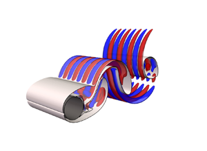
Figure 9. Normalised streamwise vorticity isocontour  ${\omega _x}/{||\boldsymbol {\omega }||_\infty }$ for mode B at $\lambda _z=0.66D$ and mode A at $\lambda _z=4D$ and ${{Re}}=350$. Red and blue iso-surfaces correspond respectively to positive and negative values of $\pm 0.1$. The translucent iso-surfaces represent the base flow vorticity at level $\pm 0.01$.

Figure 10. Streamwise vorticity distribution in an  $(x,y)$ plane of mode A and B at ${{Re}}=350$ for different Mach numbers. The fields are normalised by the maximum absolute value $\omega _{x,max}=\max (|\omega _x|)$ and the spanwise location of these planes corresponds to $\omega _{x,max}$. The black dashed line indicates the streamwise position of $\omega _{x,max}$. Black solid lines indicate the base flow vorticity contours at levels $\pm 0.1$.

Figure 11. Cross-stream vorticity distribution at  ${{Re}}=350$. Same convention as in figure 10 but considering $\omega _y$.
Overall, when moving from large to short wavelengths, the structure of the mode moves from Kármán vortices to braids in the base flow. That is, the instability transitions from an elliptic-type instability to a hyperbolic-type instability, which has also been observed for plane mixing layers (Arratia, Caulfield & Chomaz Reference Arratia, Caulfield and Chomaz2013) and round jets (Nastro, Fontane & Joly Reference Nastro, Fontane and Joly2020). Our observations show that this transition is delayed as the Mach number increases.
3.3. Energy budget analysis
To further investigate the influence of the Mach number on secondary instabilities of the cylinder wake, we conduct an energy budget analysis. The linearised equation for the perturbation velocity reads
 \begin{align} \frac{\partial\boldsymbol{u}}{\partial t} + \boldsymbol{U}\boldsymbol{\cdot}\boldsymbol{\nabla}{\boldsymbol{u}}+\boldsymbol{u}\boldsymbol{\cdot}\boldsymbol{\nabla}{\boldsymbol{U}} &= \frac{1}{R}\left(-\boldsymbol{\nabla} p+ \mu\left(\boldsymbol{\nabla}^2\boldsymbol{u}+\frac{1}{3}\boldsymbol{\nabla}\boldsymbol{\cdot}\boldsymbol{u}\right)\right)\nonumber\\ &\quad-\frac{\rho}{R^2}\left(-\boldsymbol{\nabla} P +\mu\left(\boldsymbol{\nabla}^2\boldsymbol{U}+\frac{1}{3}\boldsymbol{\nabla}\boldsymbol{\cdot}\boldsymbol{U}\right)\right), \end{align}
where  $(\boldsymbol {U},P,R)$ and $(\boldsymbol {u},p,\rho )$ indicate the base flow and perturbation primitive variables, respectively. Multiplying (3.2) by the perturbation velocity $\boldsymbol {u}$ and integrating it over the whole computational domain $V$ leads to the temporal evolution of the kinetic energy of the perturbation $\mathcal {E}=\int _V\frac {1}{2}|\boldsymbol {u}(\boldsymbol {x})|^2 \,\textrm {d}\boldsymbol {x}$:
 \begin{align} \frac{{\rm d}\mathcal{E}}{{\rm d}t}&= \overbrace{ -\int_V\boldsymbol{u}\boldsymbol{\cdot}(\boldsymbol{U}\boldsymbol{\cdot}\boldsymbol{\nabla}{\boldsymbol{u}})\,{\rm d} \boldsymbol{x}}^{\mathcal{P}_1}\overbrace{-\int_V\boldsymbol{u}\boldsymbol{\cdot}(\boldsymbol{u} \boldsymbol{\cdot}\boldsymbol{\nabla}{\boldsymbol{U}})\,{\rm d}\boldsymbol{x}}^{\mathcal{P}_2}+ \overbrace{\int_V\boldsymbol{u}\boldsymbol{\cdot}\left(\frac{\rho}{R^2}\boldsymbol{\nabla} P-\frac{1}{R}\boldsymbol{\nabla} p\right){\rm d}\boldsymbol{x}}^{\mathcal{P}_3}\nonumber\\ &\quad +\underbrace{\int_V\boldsymbol{u}\boldsymbol{\cdot}\mu\left[\frac{1}{R}\left(\boldsymbol{\nabla}^2\boldsymbol{u}+ \frac{1}{3}\boldsymbol{\nabla}\boldsymbol{\cdot}\boldsymbol{u}\right) -\frac{\rho}{R^2}\left(\boldsymbol{\nabla}^2\boldsymbol{U}+\frac{1}{3}\boldsymbol{\nabla}\boldsymbol{\cdot}\boldsymbol{U}\right) \right]{\rm d}\boldsymbol{x} }_{\mathcal{P}_4}, \end{align}
where four different terms can be identified in the right-hand side:
(i)
$\mathcal {P}_1$ comes from the advection of the perturbation by the base flow and can be reformulated as
(3.4)which corresponds to the energy production/destruction due to the base flow contraction/expansion;(ii)
$\mathcal {P}_2$ comes from the advection of the base flow by the perturbation and can be expanded in the following form:
(3.5)where$\mathcal {P}_{{st}}$ and ${\mathcal {P}_{{sh}}}$ are the energy production/destruction due to the base flow strain field and base flow shear, respectively;(iii)
$\mathcal {P}_3$ is the energy production/destruction due to the pressure gradients;(iv)
$\mathcal {P}_4$ is the viscous dissipation.


Figure 12 shows the contribution to perturbation growth rate  $\sigma _\mathcal {E}=({1}/{2\mathcal {E}})({\textrm {d}\mathcal {E}}/{\textrm {d}t})$ of the different terms of (3.3) with respect to the Mach number for mode A at Reynolds numbers ${{Re}}=250$ and ${{Re}}=350$, and for mode B at Reynolds number ${{Re}}=350$. The values of the growth rate given by the stability analysis ( $\sigma =\log (\mu )/T$) are also reported for comparison. Discrepancies between the two values of $\sigma$ and $\sigma _\mathcal {E}$ are attributed to the computation of the gradients in the reconstruction of the perturbation fields, particularly visible for the modes at small wavelengths and high Reynolds number: mode B at $\lambda _z=0.66D$ in figure 12(c) and mode A at $\lambda _z=2.5D$ in figure 12(d). Nevertheless, these differences do not change the overall trend of the different contributions.

Figure 12. Evolution with respect to the Mach number of the growth rate of the mode as well as the contribution of each term of the kinetic energy budget, according to (3.3), for (a) mode A at  $\lambda _z=3D$ and ${{Re}}=250$, (b) mode A at $\lambda _z=4D$ and ${{Re}}=250$, (c) mode B at $\lambda _z=0.66D$ and ${{Re}}=350$, (d) mode A at $\lambda _z=2.5D$ and ${{Re}}=350$, (e) mode A at $\lambda _z=3D$ and ${{Re}}=350$ and (f) mode A at $\lambda _z=4D$ and ${{Re}}=350$.
In all cases, the growth rate results from a balance between the production term  $\mathcal {P}_2$ associated with the base flow deformation and the dissipation $\mathcal {P}_4$. While the latter only slightly varies with compressibility, $\mathcal {P}_2$ is very sensitive to the increase of the Mach number and drives the growth rate variation with respect to ${{M}}_{\infty }$. This is particularly visible for mode B (decreasing) and mode A (increasing) at wavelength $\lambda _z=2.5D$ and Reynolds number ${{Re}}=350$ in figures 12(c) and 12(d). Values of $\mathcal {P}_{{sh}}$ and $\mathcal {P}_{{st}}$, which both contribute to the production term $\mathcal {P}_2$, are also reported. At ${{Re}}=250$, their values do not change significantly with respect to the Mach number, but an overall decrease of $\mathcal {P}_{{sh}}$ in favour of $\mathcal {P}_{{st}}$ is observed when the wavelength increases from $\lambda _z=3D$, in figure 12(a), to $\lambda _z=4D$, in figure 12(b). However, at ${{Re}}=350$, compressibility changes the contribution of $\mathcal {P}_{{sh}}$ and $\mathcal {P}_{{st}}$ to the growth rate of the mode as the Mach number is increased.
Figure 13 presents the contributions of  $\mathcal {P}_{st}$ and $\mathcal {P}_{sh}$ normalised by $\mathcal {P}_2$ at ${{Re}}=350$ for three representative Mach numbers. Values of ${{M}}_{\infty }=0.2$ and $0.3$ have been omitted because they are very close to those of ${{M}}_{\infty }=0.1$, which could be due to interpolation errors and therefore do not bring useful information. For each Mach number, $\mathcal {P}_{{st}}$ increases while $\mathcal {P}_{{sh}}$ decreases when moving from the smallest to the largest unstable wavelength of mode A. At the largest unstable wavelength, the energy production is entirely due to the base flow strain conversion $\mathcal {P}_{{st}}$, with $\mathcal {P}_{{sh}}$ turning negative. We can also observe that mode A instability is mainly due to the $\mathcal {P}_{st}$ contribution while that of mode B to the $\mathcal {P}_{sh}$. Moreover, compressibility increases the strain contribution and decreases the shear one at all wavelengths.

Figure 13. (a) Strain and (b) shear conversion at  ${{Re}}=350$ as a function of the wavelength for ${{M}}_{\infty }=0.1$, ${{M}}_{\infty }=0.4$ and ${{M}}_{\infty }=0.5$. The solid lines are the interpolation of the strain and shear conversion of mode A. The dashed lines delimit the range of unstable wavelengths of mode A and mode B.
4. Conclusions
Three-dimensional secondary instabilities developing in the 2-D periodic wake of the circular cylinder have been analysed at various Reynolds and Mach numbers up to  ${{Re}}=350$ and ${{M}}_{\infty }=0.5$. The 2-D time-periodic base state is found to exhibit time-averaged properties that substantially vary within the range of Reynolds and Mach numbers considered. Specifically, three different types of time-averaged flow structure of the recirculation region are identified when varying both Reynolds and Mach numbers.
Mode A and mode B secondary instabilities are obtained through a Floquet analysis, which had proven to provide consistent results also in cases where the base flow is not purely periodic in the very far wake. The increase of Mach number has a stabilising effect on both modes close to the critical thresholds, delaying the 3-D transition without modifying the spanwise wavelengths at which the flow becomes unstable. Conversely, above the critical thresholds, compressibility still has a stabilising effect on mode B but progressively becomes destabilising for mode A as the Reynolds number is further increased. The range of unstable wavelengths does not change with  ${{M}}_{\infty }$ for mode B, while it shifts towards lower values for mode A as ${{M}}_{\infty }$ is increased. Interestingly, the normalisation of the spanwise wavelengths of the modes with the characteristic length scales of the time-averaged recirculation region of the base flow highlights a correlation between properties of the unstable modes and those of the time-averaged flow field.
The vorticity distributions of mode A and mode B are also analysed with respect to the influence of compressibility. The structure of mode B remains unchanged with the increase of Mach number, while the modifications of the mode A structure induced by compressibility depends on the wavelength: the structure remains unchanged at large wavelengths but is substantially modified at small wavelengths. These changes include both a vorticity concentration in the braids and a vorticity depletion in the Kármán vortices.
Through the analysis of the perturbation energy budget, it is observed that the growth rates of both modes A and B results from the competition between the production through base flow deformation  $\mathcal {P}_2$ and the dissipation $\mathcal {P}_4$. Dissipation only varies slightly with compressibility and $\mathcal {P}_2$ is the one that drives the growth rate variations with respect to the Mach number. The production term $\mathcal {P}_2$ can be further decomposed into a base flow strain conversion term $\mathcal {P}_{{st}}$ and a base flow shear conversion term $\mathcal {P}_{{sh}}$. The mode A kinetic energy production is mainly due to the base flow strain conversion term and this term is increased by compressibility. In contrast, the mode B kinetic energy production is mainly due to base flow shear conversion term and this term is decreased by the compressibility. These observations may be useful to elucidate on why mode A is destabilised by compressibility while mode B is stabilised.
Beyond the present work, it would be interesting to extend this analysis to the quasi-periodic (QP) 3-D mode that emerges in the cylinder periodic wake at higher Reynolds numbers, i.e.  ${{Re}}\geq 380$ (Blackburn et al. Reference Blackburn, Marques and Lopez2005). The investigation of compressibility effects beyond ${{M}}_{\infty }=0.5$ in the transonic and supersonic regime, as done by Sansica et al. (Reference Sansica, Robinet, Alizard and Goncalves2018) for the flow past a sphere, could be also considered.
Funding
This work was in part supported by the French Ministry of Defence through financial support of the Agence Innovation Défense (grant 2021 65 0070) and performed using HPC resources from GENCI-IDRIS and GENCI-CINES on Jean Zay, Occigen (grant A0082A07178) and CALMIP on Olympe (grants 2021-p1425 and 2022-p1425).
Declaration of interests
The authors report no conflict of interest.
Appendix A. Mesh convergence study
Figure 14 shows the mesh convergence study for the 2-D base flow monitored through the evolution of both the time-averaged drag coefficient  $C_D$ and the Strouhal number ${{St}}$ with respect to the grid characteristic size ( $1/N_{{cells}}$) of five different meshes, from M1 the coarsest to M5 the most refined. M3 has been chosen for the 2-D resolution showing less then $0.5\,\%$ of error with respect to the Richardson extrapolated value (red dot) on the drag coefficient and a $0.1\,\%$ error on the Strouhal number. Values of the Floquet exponent $\mu$ with respect to the discretisation in the $(x,y)$ plane and $\varDelta _z=D/8$ are shown in figure 15. Results obtained with mesh M3 differ by less than $1\,\%$ for mode A and $3\,\%$ for mode B. In table 1, results for modes A and B at other wavelengths are also reported, including the influence of the spanwise discretisation. The relative error for mode A between mesh M3 with $\varDelta _z=D/8$ and M5 with $\varDelta _z=D/32$ is ${\approx }0.5\,\%$, while that for mode B between mesh M3 with $\varDelta _z=D/8$ and M5 with $\varDelta _z=D/32$ is ${\approx }1.5\,\%$. The higher relative error observed for mode B is due to its shorter wavelength to that of mode A. Results at ${{Re}}=300$ and ${{M}}_{\infty }=0.05$ using mesh M3 and $\varDelta _z=D/8$ are also reported in figure 16 for all the wavelengths and compared with results from (Leontini et al. Reference Leontini, Lo Jacono and Thompson2015), showing good agreement. Based on these results, mesh M3 with $\varDelta _z=D/8$ has been chosen.

Figure 14. Convergence on (a) drag coefficient  $C_D$ and (b) Strouhal number ${{St}}$ with respect to five different meshes at ${{Re}}=300$. M1 is the coarsest, M5 the most refined. Here, $\textrm {M}^*$ (red dots) represents the asymptotic value as given by Richardson extrapolation. Henderson (Reference Henderson1995) reported $C_D\approx 1.4$.

Figure 15. Convergence on the Floquet exponents for (a) mode A at a wavelength  $\lambda _z=4D$ and (b) mode B at a $\lambda _z=0.8D$ with respect to five different $(x,y)$-resolutions and $\varDelta _z=0.125D$ at ${{Re}}=300$ and ${{M}}_{\infty }=0.05$. Red dots correspond to the Richardson extrapolation.
Table 1. Floquet exponents for mode A at a wavelength  $\lambda _z=4D,3D$ and mode B at $\lambda _z=0.8D,0.75D$ with respect to different resolutions at ${{Re}}=300$ and ${{M}}_{\infty }=0.05$.


Figure 16. Results at  ${{Re}}=300$ and ${{M}}_{\infty }=0.05$ using mesh M3 with $\varDelta _z=D/8$ compared with the results taken from Leontini et al. (Reference Leontini, Lo Jacono and Thompson2015). Dashed grey line represents the interpolation curve of the present results.
Appendix B. Influence of the starting time within the limit cycle
The influence of the base flow initial instant within the period  $T$ on both modes A and B Floquet multipliers is reported in figure 17, together with the lift coefficient ( $C_L$) evolution along the period $T$ of the base flow. The Floquet multipliers exhibit a sinusoidal evolution with respect to the base flow starting point, with fluctuations of approximately $0.5\,\%$ around the mean value. The evolution is out of phase for mode A and in phase for mode B with respect to the $C_L$ evolution. These simulations have been performed on the coarsest mesh M1 with $\varDelta _z=D/8$.

Figure 17. Effect of the base flow starting point on mode A and mode B Floquet multipliers with respect to the lift coefficient evolution at  ${{Re}}=300$ and ${{M}}_{\infty }=0.05$.
Appendix C. Base flow aperiodicity
The main assumption underlying Floquet theory is the periodicity of the base state. This assumption allows to consider the periodic limit cycle as a fixed point on the Poincaré section and therefore to have a constant Jacobian matrix at each period  $T$. In wake flows, such as the case discussed in this work, the base state is indeed periodic in the near wake downstream of the cylinder as a consequence of vortex shedding, with period $T=1/f$. However, in the far wake, where vortex pairing can occur (figure 18a), the base state may no longer be $T$-periodic, as shown by the velocity field difference between the unsteady solution at times $t$ and $t+T$ in figure 18(b). Some recent works have discussed this limitation and provided some methodologies to ensure that the base state remains $T$-periodic in the whole numerical domain. This can be achieved either by reconstructing the base flow solution and limiting the downstream extent of the numerical domain for the stability calculation (Lo Jacono et al. Reference Lo Jacono, Leontini, Thompson and Sheridan2010), or by computing and using phase-averaged or stabilised base flows (Jiang Reference Jiang2021). These methods induce modifications of the unsteady base flow solution, not fully representative of the actual flow. With the method adopted in this work, the base flow is integrated in time with the perturbation as indicated by (2.13), preventing from using these approaches. Nevertheless, it is possible to assess the relevance of the stability analysis performed here even if the base flow is only approximately periodic in the far wake. To investigate the influence of the far-wake aperiodicity of the base flow, results of Floquet analysis at two Reynolds and Mach numbers using base flows computed at different periods are reported in figure 19. These spectra highlight that mode A and mode B ( $\mu _r>0$ and $\mu _i=0$) are not affected by the base flow aperiodicity in the far wake because their Floquet multipliers do not vary for the different base state and their spatial structures are located in the periodic near-wake region, as shown in figure 18(c) for the least stable mode at ${{Re}}=300$ and ${{M}}_{\infty }=0.05$. Conversely, the modes in the lower part of the spectrum ( $\mu _r<0$) show a dependence on the chosen period of the base flow and their spatial structures are located in the far wake, as shown in figure 18(d), where the base flow is no longer $T$-periodic. Hence, to analyse the far-wake instabilities, which have not been considered in this work, approaches like those cited above should be used.

Figure 18. (a) Normalised base flow velocity magnitude  $U/U_\infty$ at ${{Re}}=300$, ${{M}}_{\infty }=0.05$ and (b) velocity magnitude field difference between base flow at times $t$ and $t+T$. (c) Example of mode not affected by aperiodic zone and (d) example of wake mode developing in the aperiodic region.

Figure 19. Spectra obtained with different base states periods at (a)  ${{Re}}=300$, ${{M}}_{\infty }=0.05$ and (b) ${{Re}}=350$, ${{M}}_{\infty }=0.3$. Solid black line indicates the unitary circle.


