


1. Introduction
A variety of physical phenomena in nature involve the dynamics of particles immersed in fluid media. Geosciences, astrophysics, the chemical industry, mineral treatment and material sciences are some of the disciplines that encompass the study of the interactions of discrete systems with fluid flow. Segregation of granular matter, asteroid penetration into the atmosphere, sediment transport in natural systems, handling of mineral grains in the mining industry, are some engineering applications where this is particularly relevant. This type of system is usually studied from a hydrodynamic perspective using the forces acting on the surface of the body. This involves analysing the drag coefficient  $C_D=2\,|\boldsymbol {F}_D|/(\rho _f\,|\boldsymbol {u}_\infty |^{2}\,A_p)$ as a dimensionless quantity capable of describing the resistance force exerted by the body within a fluid medium, where $\boldsymbol {F}_D$ is the drag force exerted on the body, $\rho _f$ is the density of the fluid, $\boldsymbol {u}_\infty$ is the terminal or free-stream velocity of the fluid, and $A_p$ is the projected area of the body on a plane normal to the direction of the fluid flow.
The importance of the drag coefficient lies in the optimisation and understanding of the fluid dynamics or the rheological behaviour of solid bodies within a fluid medium. Its engineering applications extend to aerodynamic design of vehicles (Bayındırlı & Çelik Reference Bayındırlı and Çelik2018), net design in aquaculture and oceanography (Tsukrov et al. Reference Tsukrov, Drach, Decew, Swift and Celikkol2011), optimisation of pneumatic transport in the food industry (Defraeye, Verboven & Nicolai Reference Defraeye, Verboven and Nicolai2013), and hydrodynamic behaviour of plant layers (Etminan, Lowe & Ghisalberti Reference Etminan, Lowe and Ghisalberti2017), among others. Oggiano et al. (Reference Oggiano, Saetran, Løset and Winther2004) performed an interesting application of drag in the aerodynamic behaviour of athletes, determining the influence of surface roughness on resistance at high Reynolds numbers, and how these results extrapolate to drag on rough cylinders.
Nevertheless, the dynamics of the external flow has been analysed from fundamental geometries from both analytical and experimental perspectives. Pioneering studies have determined the influence of drag on spherical bodies (Achenbach Reference Achenbach1972; Haider Reference Haider1989; Constantinescu & Squires Reference Constantinescu and Squires2004; Sun et al. Reference Sun, Saito, Takayama and Tanno2005) as a basis for extending it to more complex geometries, as ellipsoids (Ouchene et al. Reference Ouchene, Khalij, Tanière and Arcen2015; Sanjeevi & Padding Reference Sanjeevi and Padding2017; Sanjeevi, Kuipers & Padding Reference Sanjeevi, Kuipers and Padding2018), spherical clusters (Tran-Cong, Gay & Michaelides Reference Tran-Cong, Gay and Michaelides2004), cylinders (Lam & Lin Reference Lam and Lin2009; Cadot et al. Reference Cadot, Desai, Mittal, Saxena and Chandra2015), agglomerates (Chen, Chen & Fu Reference Chen, Chen and Fu2022) and granular media (Guillard, Forterre & Pouliquen Reference Guillard, Forterre and Pouliquen2014; Jing et al. Reference Jing, Ottino, Umbanhowar and Lueptow2022).
In general, the drag coefficient depends on the Reynolds number  $Re$, especially for $Re<10^4$; above this value, the drag coefficient remains practically constant due to the transition to turbulence. Additionally, for smooth bodies (such as spheres and cylinders) in highly turbulent flows, there is also a drag crisis, where the drag coefficient decreases drastically up to a critical value, beyond which it then increases gradually with increasing $Re$ until reaching a relatively constant value. This drag crisis is related to the turbulent transition of the boundary layer when $Re$ is relatively large. However, its existence and the behaviour during this transition have not been shown for irregularly shaped particles, despite initial evidence showing that.
This phenomenon has been of interest to understand the behaviour of the drag coefficient beyond smooth geometries. Beratlis, Balaras & Squires (Reference Beratlis, Balaras and Squires2019) carried out a set of direct numerical simulations (DNS) to determine the origin of drag patterns around dimpled spheres at post-critical  $Re$. They found that the dimples, although reducing the critical value of the Reynolds number relative to that of the smooth sphere, impose a local drag penalty, which contributes significantly to the overall drag force.
The effect of rotational dependence of smooth bodies on drag is described well by Sanjeevi & Padding (Reference Sanjeevi and Padding2017), who derived a periodic behaviour of the drag coefficient as the ellipsoidal particle is rotated under the circumstance where its longest axis, shortest axis and flow directions are always on the same plane, for  $Re$ up to 2000. However, many questions about the influence of surface irregularity and the complete randomness of rotation on the fluid dynamic behaviour of the particle remain to be resolved, especially again under turbulent regimes.
Regarding the analysis of drag in irregularly shaped particles, the difficulty lies in the morphological description of the particle. Different shape factors have been described to encompass the geometry of irregular particles and base their analysis on these factors. Dioguardi, Mele & Dellino (Reference Dioguardi, Mele and Dellino2017) presented a model capable of describing the drag coefficient of irregularly shaped particles from the sphericity and circularity of the geometries, in a wide range of  $Re$ (0.03–10 000). Sommerfeld & Qadir (Reference Sommerfeld and Qadir2018) used these shape factors and applied the lattice Boltzmann method with local grid refinement on non-spherical irregular geometries at $Re$ up to 200, finding patterns similar to spherical bodies in both drag and lift. Some applications of drag on irregularly shaped particles have been analysed by Sun et al. (Reference Sun, Zhao, Peng, Wang, Jiang and Yu2018) and Wang et al. (Reference Wang, Zhou, Wu and Yang2018).
The irregularity of the particle surface directly impacts the drag coefficient. Zhang et al. (Reference Zhang, He, Xie, Wei, Li, Wang and Wang2023) proposed various drag coefficient models for irregularly shaped particles for  $Re\leq 200$. They determined that $C_D$ increases as the particle surface becomes more irregular. They also showed that $C_D$ varies slowly at low Reynolds numbers for different fluid incidence angles, while it does so more rapidly at high $Re$. However, they did not study the behaviour for very large $Re$.
$Re$.
Gai & Wachs (Reference Gai and Wachs2023) explored the influence of the angularity of Platonic bodies on drag and lift coefficients. Their findings highlight that at low Reynolds numbers, the cross-sectional area of the particle has a high influence on the drag coefficient, while at high Reynolds numbers, the angular position of the particle with respect to the flow tends to have a greater influence.
Recently, Michaelides & Feng (Reference Michaelides and Feng2023) performed a complete review of the different models to estimate the drag coefficients for both symmetrical particles and irregularly shaped particles. In the review, they critically discuss the advantages and difficulties when using descriptors and shape factors in particle morphology, and its different applications and restrictions when evaluating these correlations in computational fluid dynamics (CFD) codes.
The objective of this study is to contribute to the characterisation of the fluid dynamic behaviour of irregularly shaped particles in a wide spectrum of flow regimes  $Re=1\unicode{x2013}10^7$, and unravel the rotational dependence effect on the drag coefficient. This paper is divided into the following sections. In § 2, we describe the CFD tools applied to resolve pressure and velocity fields, within the set-up geometry, both for model validation and for obtaining the drag forces for irregular geometries. The results of the drag and the rotational influence for the range of laminar and turbulent flow are presented in § 3, highlighting and discussing the different findings of the fluid dynamic behaviour of the drag for this type of geometry. The main conclusions of this research are summarised in § 4.
2. Methods
2.1. Numerical resolution and geometric considerations
The flow development is computed by solving numerically the Navier–Stokes equations for viscous, incompressible and isothermal flow:
 $$\begin{gather} \boldsymbol{\nabla} \boldsymbol{\cdot} \boldsymbol{u}=0, \end{gather}$$
 $$\begin{gather}\rho_f(\boldsymbol{u}\boldsymbol{\cdot} \boldsymbol{\nabla})\boldsymbol{u}=\boldsymbol{\nabla}\boldsymbol{\cdot}[{-}pI+\mu_f(\boldsymbol{\nabla} \boldsymbol{u}+(\boldsymbol{\nabla} \boldsymbol{u})^{\rm T})], \end{gather}$$
where  $\boldsymbol {u}$ is the velocity field inside the fluid domain, $\rho _f$ is the fluid density, $\mu _f$ is the fluid dynamic viscosity, and $p$ is the pressure field in the system.
The flow regime at high  $Re$ is evaluated using the Reynolds-averaged Navier–Stokes (RANS) turbulence model applied to the transport equations for shear stress ( $k$-
$k$- $\omega$) viscous model (Menter Reference Menter1994). Although its capacity to resolve turbulent elements in the boundary at high Reynolds numbers has been investigated, some authors hold the view very good accuracy may not obtained by RANS-based CFD, and often the numerical solution is partly to blame for the errors. This latter problem will be solved by fine grid or mesh refinement in the fluid region, and increased computing power, although the convergence may be difficult (Roy et al. Reference Roy, Payne, McWherter-Payne and Salari2006). Compared with other advanced CFD methods, i.e. DNS and large-eddy simulations, the RANS model is computationally less expensive, facilitating the possibility of systematic study on rotation-angle-dependent drag coefficients of irregularly shaped grains under various Reynolds number in this study. Further, according to Yang et al. (Reference Yang, Gupta, Kuo and Gopalakrishnan2014), RANS simulation is good enough for capturing overall flow trends; however, if one is interested in getting reasonably accurate estimates of velocity magnitudes, flow structures, turbulence magnitudes and their distributions, then one must resort to other advanced CFD simulations. In this study, our focus is on the overall drag force on the grain rather than on comparing the flow structures induced by rotation angles. Validations from both numerical (DNS for the irregularly shaped grain) and experimental (the spherical grain) investigations for our RANS results will be given in the following sections.
The numerical resolution is obtained from the pressure–velocity coupled scheme (based on pressure), which allows the simultaneous resolution of the equations of motion and continuity, ensuring greater robustness of the numerical solution. The spatial discretisation follows a second-order method, given the irregular flow conditions in the boundary layer, especially in the turbulent regime at extremely high  $Re$.
$Re$.
The irregular geometries of the grains were created from a practical method for generating irregularly shaped particles using a fractal dimension as a descriptor parameter of the grain morphology. It uses spherical harmonics that allow us to define and control the morphology of the particle from its fractal properties – its shape, roundness and texture – based on the model presented by Wei et al. (Reference Wei, Wang, Nie and Zhou2018). The generated irregularly shaped particles used in this paper are shown in figures 1(a,b).

Figure 1. Geometry of irregularly shaped particles used in the study of the drag coefficient. (a) Grain with fractal dimension  $D_f=2.287$, typically frequent for Leighton Buzzard sand. (b) Grain with fractal dimension $D_f=2.420$, frequent for highly decomposed granite.
The particles are characterised by their axial asymmetry caused by the presence of dimples and ridges distributed randomly over their entire surface. The fractal dimension  $D_f$ is 2.287 and 2.420 for the two grains, typically frequent for Leighton Buzzard sand (LBS) in Bedfordshire, and highly decomposed granite (HDG), respectively. Those values are based on the statistical relationship between the spherical harmonic descriptor and the spherical harmonic degree. The characteristic lengths in the longest, intermediate and shortest dimensions of a box containing the particle inside are 2.87 mm, 2.49 mm and 2.05 mm for LBS, and 5.12 mm, 3.02 mm and 2.96 mm for HDG grain. Table 1 summarises the main shape descriptors for both particles; the definitions are based on those presented by Angelidakis et al. (Reference Angelidakis, Nadimi and Utili2022) and Michaelides & Feng (Reference Michaelides and Feng2023).
Table 1. Particle shape descriptors of Leighton Buzzard sand and highly decomposed granite, based on the definitions presented in Angelidakis, Nadimi & Utili (Reference Angelidakis, Nadimi and Utili2022) and Michaelides & Feng (Reference Michaelides and Feng2023). The flatness is herein defined as the ratio between the lengths of the major and intermediate axes; the elongation is defined as the ratio between the lengths of the intermediate and minor axes; the compactness is defined as the ratio of the area of the particle to the square of its maximum perimeter; and the sphericity is defined as the ratio of the surface area of the sphere with equivalent volume to the actual surface area of the particle.

We define the Reynolds number based on the projected area-equivalent particle diameter  $d_p$ as $Re=\rho _f\,|\boldsymbol {u}_\infty |\,d_p/\mu _f$. The equivalent diameter of the irregularly shaped particle is obtained from the diameter of a circumference with the same equivalent projected area of the particle, $A_p$, on the plane perpendicular to the fluid flow, $d_p=\sqrt {4A_p/{\rm \pi} }$.
2.2. Numerical set-up and grid resolution influence
The configuration applied in the simulations emulates those developed in physical experimentation, with a solid body inside a wind tunnel through which the fluid flows and where the resulting forces on the surface of the body under study are analysed. Figure 2(a) shows the computational domain used in all the simulations. These dimensions were chosen to avoid any influence of the geometry walls.

Figure 2. (a) Computational domain used in the numerical study, whose dimensions make it possible to avoid the influence of the fluid–wall interaction on the fluid–particle interaction (not to scale). (b) Unstructured mesh applied in conjunction with inflation methods to optimise turbulence capture in the boundary layer. (c) Azimuthal rotation  $\alpha$ anticlockwise with respect to the $z$-axis ( $x$–
$x$– $y$ meridional plane). (d) Polar rotation $\beta$ anticlockwise with respect to the $y$-axis ( $x$–
$x$– $z$ meridional plane).
We adopt the boundary conditions considering the inlet flow at free-stream velocity by setting  $u_x=u_{inlet}$ and $u_y=u_z=0$, which are also for a no-slip condition in the walls. A pressure outlet past the irregularly shaped grain is given by setting $p=0$ and ${\rm d}{u_x}/{{\rm d}\kern0.7pt x}={\rm d}{u_y}/{{\rm d}\kern0.7pt x}={\rm d}{u_z}/{{\rm d}\kern0.7pt x}=0$, while $u_x=u_y=u_z=0$ is set in the fluid–solid interface.
To determine the resolution of the modelling grid, the calibration is performed by running 27 simulations, and using an isolated smooth sphere and comparing its drag coefficient as a function of Reynolds number with the experimental values obtained by Achenbach (Reference Achenbach1972). Critically, we concentrate on the size of the mesh around the particle in order to capture the boundary layer effects even at high Reynolds numbers. Figure 2(b) shows the meshing detail in the zone close to the boundary layer, where the thick black line represents the refinement required to capture the information at the boundary between the irregularly shaped grain and the fluid (smaller mesh elements).
The analysis of the rotational dependence of the drag coefficient is performed considering two types of particle rotation respect to the fluid flow: azimuthal rotation  $\alpha$ (anticlockwise with respect to the $z$-axis on the meridional $x$–
$x$– $y$ plane), and polar rotation $\beta$ (anticlockwise with respect to the $y$-axis on the $x$–
$x$– $z$ plane) as shown in figures 2(c,d). Formally, let $[x_0\quad y_0\quad z_0 ]^{\rm T}$ be the original coordinates of the points on the surface of the particle, and the updated coordinates of said points, $[x_u\quad y_u\quad z_u ]^{\rm T}$, once the particle is rotated, are given by
 \begin{equation} \begin{bmatrix} x_u\\ y_u\\ z_u \end{bmatrix}=\begin{bmatrix} \cos \beta & 0 & -\sin \beta\\ 0 & 1 & 0\\ \sin \beta & 0 & \cos \beta \end{bmatrix}\times \begin{bmatrix} \cos \alpha & \sin \alpha & 0\\ -\sin \alpha & \cos \alpha & 0\\ 0 & 0 & 1 \end{bmatrix}\times \begin{bmatrix} x_0\\ y_0\\ z_0 \end{bmatrix}. \end{equation}
 For the first analysis, the complete rotation of the azimuthal angle is considered (from 0 to 2 ${\rm \pi}$, varying the angle every ${\rm \pi} /6$, totalling 13 simulations for each $Re$) following the rotation matrix $\mathfrak{R}_1=(\alpha,0)$, while a statistical analysis based on the Weibull statistics is performed to consider the combined effect of azimuthal and polar rotations according to the ordered pair $\mathfrak{R}_2=(\alpha,\beta )$ with randomly distributed values.
Figure 3(a) shows the comparison of the numerical model and the experimental data applied to the smooth sphere, obtained by Achenbach (Reference Achenbach1972) and fitted by Turton & Levenspiel (Reference Turton and Levenspiel1986). The presence and good fitting of the drag crisis is reported at  $Re>3\times 10^5$. This result allows us to determine the resolution of the mesh, where as $Re$ increases, the size of the cells of the mesh needs to be smaller to capture the turbulent behaviour in the boundary layer and the wake zone. The mesh ratio $x/d_p$ is used, with $x$ being the characteristic length of each mesh element on the particle surface, and the red dashed line in figure 3(a) shows the maximum mesh size required to obtain reasonable results, whose percentage difference does not exceed 0.25 %. This translates, for the different simulations, into a range of element numbers from 700 000 (for low $Re$) to more than 3 000 000 mesh elements (for extremely high $Re$). Figure 3(b) shows the good correlation between the predicted and measured data for the drag coefficient when using this largest mesh size. The consistency between widely accepted and simulated drag coefficients for spherical grains demonstrated that the RANS model could achieve satisfactory results as long as the mesh refinement in the fluid region is carefully conducted.

Figure 3. (a) Drag coefficient  $C_D$ as a function of the Reynolds number $Re$ for an isolated smooth sphere. The solid black line represents the fitted experimental values for the smooth sphere (Turton & Levenspiel Reference Turton and Levenspiel1986). The circles represent each numerical simulation. The red dashed line corresponds to the mesh resolution, showing a dependence on $Re$. (b) Percentage difference between experimental data and numerical results (in triangles).
3. Results
3.1. Effect of the Reynolds number
Figure 4(a) shows the drag coefficient  $C_D$ as a function of $Re$ at different flow incidence angles (azimuthal rotation $\alpha$) for the LBS and HDG grains. Therein, two extra data points from DNS are also given. They agree well with those from the corresponding RANS simulations. Notably, considering the high number (426) of simulations across seven orders of Reynolds number, it is not possible to run all our simulations using DNS, so we just provide two validation cases for illustrative purposes. In general, the drag coefficient decreases up to values $Re\approx 10\,000$ (subcritical regime). Between these $Re$ values and the drag crisis, $C_D$ is independent of the flow regime. Within this zone, the drag coefficient is usually greater than that of the sphere (solid black line in figures 4a,b) for any incidence angle $\alpha$, despite having the same decreasing behaviour. This shows the influence of the irregularity of the particle surface, altering the flow conditions inducing irregularities in the streamline patterns. As for smooth spheres, the irregularly shaped particle also suffers a drag crisis with an abrupt decrease of the drag coefficient for values $Re\approx 100\,000$. In fact, as is observed for dimpled and rough spheres, the irregularly shaped grain causes a more sudden drop of the drag coefficient, compared to the smooth sphere. This means that the roughness of the surface displaces the boundary layer, causing the drag coefficient to reach its critical value at lower Reynolds numbers ( $Re_{cr,sphere}>Re_{cr,grain}$). Figure 4(b) presents the drag crisis for the LBS particle, compared to the smooth sphere. It can be observed that the minimum values of the drag coefficient are larger than those of the smooth sphere ( $C_D\approx 0.07$). After this crisis, $C_D$ increases again until it is practically independent of the Reynolds number, but dependent on the incidence angle (see the coloured symbols). In summary, a common pattern of the existence of the four flow mechanism zones in terms of $C_D$ arises: (1) subcritical, where $C_D$ decreases as $Re$ increases ( $Re<10^5$); (2) critical, where $C_D$ decreases sharply with growing $Re$ ( $10^5< Re<2 \times 10^5$); (3) supercritical, beyond the lowest value of $C_D$, where it increases slightly with increasing turbulence ( $2 \times 10^5< Re<10^6$); and finally (4) transcritical, where $C_D$ is practically constant at very high values $Re>10^6$.

Figure 4. (a) Drag coefficient  $C_D$ as a function of the Reynolds number $Re$ for the LBS and HDG grains. The black solid line represents the values for the smooth sphere. The markers represent the different simulations performed. The coloured symbols shows the range of values of the azimuthal rotation $\alpha$. (b) Drag coefficient $C_D$ as a function of the Reynolds number $Re$ in the drag crisis.
3.2. Effect of the incidence angle
Figure 5(a) represents the behaviour of the drag coefficient as a function of the azimuthal rotation  $\alpha$, for different Reynolds numbers. It clearly shows that as the angle of rotation changes, the drag coefficient increases up to a maximum value. This behaviour reverses as the angle continues to change, repeating itself, similarly to a periodic pattern. This phenomenon is directly associated with the variation of the surface area exposed to the fluid flow. In this case, the minimum projected area coincides with $\alpha =0$, where the lowest value of the drag coefficient is obtained, repeating the pattern every 180 $^{\circ }$. Thus as the particle is rotated (increase in $\alpha$), the drag coefficient increases until it reaches its maximum value when the projected area by the grain is maximum (figures 5a,b). This is also under the condition that the grain rotation is executed in the same way as was done with the previous studies of drag in ellipsoids, where such a periodic pattern is satisfied. However, this result does not necessarily indicate that two particles with the same projected area exposed to the flow experience the same drag. Due to the fractal nature of grains, the projected area value on the macro-scale does not necessarily present a ${\rm \pi}$ pattern. However, the local characteristics of the fluid flow around the particle present self-affine similarity at the macro-scale, explaining the ${\rm \pi}$-periodicity of the drag coefficient. As can be seen in figure 5(d), there is no direct correlation between the drag coefficient and the projected area by the particle. This interesting result is closely related to the fact that a ${\rm \pi}$-periodicity is correlated with the constraint where the flow direction is parallel to the maximum projected area. Sanjeevi & Padding (Reference Sanjeevi and Padding2017) interpreted the dynamics of this periodic phenomenon in spheroids as an interesting pressure pattern effect imposed by the drag pressure over viscous pressure, especially at high $Re$.
$Re$.

Figure 5. (a) Drag coefficient  $C_D$ as a function of the angle of incidence of the flow $\alpha$ at different $Re$ for the LBS and HDG grains. (b) Normalised projected area $A_P/ {\rm \pi}r_{d}^2$ as a function of the rotation angle of incidence $\alpha$ (with $\beta =0$) for both particles. (c) Normalised drag coefficient $C_D^*$ as a function of the angle of incidence of the flow $\alpha$ at different $Re$. The solid line represents the sine-squared function. (d) Drag coefficient $C_D$ as a function of the normalised projected area $A_P {\rm \pi}r_{d}^2$, at various Reynolds numbers $Re$. The inset shows these values for HDG grains.
To better elucidate the rotational dependence, a normalised drag coefficient, defined as  $C_D^*\equiv (C_{D,a}-C_{D,min}) /(C_{D,max}-C_{D,min})$ is derived to help us to understand the relationship between the variables. In this case, $C_{D,min}$ is equal to $C_{D,\alpha =0}$, but in general, it would be defined as the minimum value in the plot shown in figure 5(a), with another orientation chosen as the initial one. Here, $C_{D,max}$ represents the maximum value. Figure 5(c) presents $C_D^*$ as a function of the azimuthal incidence angle $\alpha$, confirming the cyclic nature, but also, critically almost removing the effect of $Re$.
$Re$.
In fact, we observe that this normalised drag coefficient is also represented by a sine-squared drag law (3.1) similarly to ellipsoids. This finding allows the understanding of the hydrodynamics of discrete irregularly shaped particles and facilitates the estimation of the drag coefficient of different geometries based on the orientation of the particle with respect to the fluid flow:
 \begin{equation} C_D=C_{D,min}+(C_{D,max}-C_{D,min})\sin^{2} \alpha. \end{equation}
 A statistical analysis has been developed considering thirty random combination values for both the azimuthal rotation angle  $\alpha$ and the polar angle $\beta$ for both grains. Figures 6(a–e) show the distributions of the values of the drag coefficient for four different Reynolds numbers ( $Re=1, 100, 1000, 10\,000$), in both the laminar and turbulent regimes. In the following, we prove that the phenomenon follows a Weibull distribution Weibull (Reference Weibull1951).

Figure 6. Weibull probability density distributions of the drag coefficient for different random angles of incidence ( $\alpha \neq \beta \neq 0$): (a) $Re=1$, (b) $Re=100$, (c) $Re=1000$, (d) $Re=10\,000$, for the LBS grain; (e) $Re=10\,000$ for the HDG grain. (f) Plot of $\ln [\ln (1/P_S)]$ versus $\ln (C_D/C_{D,0})$, where $P_S$ is the survival probability distribution.
Hypothesising a Weibullian behaviour of the drag coefficient, we can define its probability density function  $PDF(C_D)$ as
 \begin{equation} PDF(C_D)=\frac{m}{\lambda}\left ( \frac{C_D}{\lambda} \right )^{m-1}\exp \left [ -\left ( \frac{C_D}{\lambda} \right )^m \right ],\quad C_D>0, \end{equation}
where  $C_D$ is the value of the drag coefficient, and $m$ and $\lambda$ are the shape and scale parameters of a specific Weibull distribution, respectively. Thus the cumulative distribution function of the drag coefficient ${CDF}(C_D)$, and the survival probability function $P_s(C_D)$, can be read as
 $$\begin{gather} {CDF}(C_D)=1-\exp \left [ -\left ( \frac{C_D}{\lambda} \right )^m \right ],\quad C_D>0, \end{gather}$$
 $$\begin{gather}P_S(C_D)=1-{CDF}(C_D)=\exp \left [ -\left ( \frac{C_D}{\lambda} \right )^m \right ],\quad C_D>0, \end{gather}$$
where  $\lambda$ could be approximated by a characteristic drag coefficient $C_{D,0}$ with $P_S(C_{D,0})\approx 37\,\%$. Finally, (3.3b) can be described in logarithmic terms as
 \begin{equation} \ln [\ln (1/P_S)]=m\ln(C_D)-m \ln (C_{D,0}). \end{equation}
From (3.4), it is possible to find the parameters of the Weibull modulus  $m$ as shown in figure 6(f). The large $R^2$ ( $>0.975$) values show the fidelity of the Weibullian behaviour.
3.3. Boundary layer separation and turbulence
One of the characteristics of external flows is the existence of a thin layer between the solid body and the fluid. This boundary layer varies depending on the flow regime and the surface of the solid body. In the case of smooth spheres, it is well studied that boundary layer separation occurs at approximately 80 $^{\circ }$ (relative to flow direction) in the subcritical regime (prior to drag crisis), and 120 $^{\circ }$ in the supercritical regime (Achenbach Reference Achenbach1972). However, in irregularly shaped particles, more than one separation point is possible, and there is ambiguity in defining the separation line, so we restrict ourselves here to show its existence in the turbulent regime. In figure 7, we present the turbulence patterns in the critical regime, at $Re=100\,000$. The influence of the irregularity of the particle surface in the separation of the boundary layer can be observed, where defining its geometry precisely is complex, considering the flow patterns in it. Thus in figures 7(a,c,e), the pattern of the vorticity isosurfaces is shown, where its increase occurs mainly at the poles of the particle, giving rise to the separation of the boundary layer. Figures 7(b,d,f) represent the velocity field contours, highlighting the formation of turbulence and the chaotic pattern behind the particle. It is important to discuss that due to the irregularity of the particle surface, there may be an artificial separation of the boundary layer when the surface is not smooth, despite the fact that it is irregular on a larger scale. In figure 7(f), it can be seen that there is more than one boundary layer separation at small scale, characterised by zones of low to zero velocity, which reflects the difficulty of quantifying the effect of turbulence on the global dynamic behaviour of the particle.

Figure 7. Turbulence patterns of (a,b) the sphere, (c,d) the LBS particle, and (e,f) the HDG particle, for  $Re=100\,000$. Here, (a,c,e) represent the vortex isosurfaces around the sphere and the irregular particles, and (b,d,f) are the velocity fields on a meridional plane.
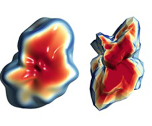
Figures 8(a,c) show the pressure patterns at  $Re=100\,000$. The high-pressure points are concentrated on the front face that is normal to the flow, impacting the grain directly on the entire perpendicular area exposed to the fluid. Figures 8(b,d) show the shear stresses for the same regime for both irregularly shaped grains. Here, the points that experience the most shear coincide with the points of least pressure. This phenomenon occurs due to the characteristics of the boundary layer, which allows the flow lines to be displaced by ‘dragging’ the fluid around the particle surface.

Figure 8. Pressure profiles on the front surface of the flow for (a) the LBS particle, and (c) the HDG particle. Shear profiles on the front surface of the flow for (b) the LBS particle, and (d) the HDG particle. The figures correspond to turbulent flow in the critical regime  $Re=100\,000$.
4. Conclusions
The drag coefficient  $C_D$ of irregularly shaped particles in a wide range of $Re$ and flow incidence angles was studied. At high $Re$, we show the existence of the drag crisis for this type of geometry, a well-described and understood phenomenon for bodies of simple geometry. However, for both geometries it is shown that $Re_c$ is lower than that for the sphere, accelerating this crisis. The angle of incidence shows a periodic behaviour of the drag coefficient with respect to the azimuthal angle of incidence of the flow, and fits to a sine-squared function. This also occurs even at very high Reynolds numbers (turbulence regime), thus extending the model described previously for spheroids, ellipsoids and smooth shapes within the laminar regime. The value of the drag coefficient can therefore be estimated for any angle of rotation (around the same axis) knowing only two values – in this case, a minimum value and a maximum value – using the suggested normalised definition of the drag coefficient $C_D^*$. The separation of the boundary layer in irregular bodies is characterised by flow patterns that are not well defined due to the irregularity of the particle surface, but which rely directly on the regularity of the surface in front of the flow, inducing the formation of vortices and eddies past flow depending on the degree of separation of the boundary layer.
Finally, the orientational dependence of the drag coefficient satisfies the Weibull behaviour, caused by both the randomness of the rotation and the position of the particle in the flow.
With this, we hope to inject interest in the study of the hydrodynamic behaviour of irregularly shaped particles, to extend its knowledge and encourage the analysis of highly turbulent flows around irregular bodies. This will also be useful to endless applications in geosciences and different disciplines of engineering.
Funding
This work is part of the support granted by the National Scientific Research Agency of Chile – Grant for Doctoral Studies no. 62210003 for Á.V., and by the Australian Research Council (ARC) – the Discovery Early Career Award (DECRA) no. DE240101106 for D.W. The corresponding author D.W. thanks Alexander von Humboldt Foundation for providing the Humboldt Fellowship hosted in RWTH Aachen. The authors thanks Professor C. Zhai in Xi'an Jiaotong University, China, for providing the ANSYS® Fluent® licence and computational resources via the Open Research Funding no. SV2021-KF-28. Associate Professor Y. Gan is thanked for the inspired and fruitful discussions of this study.
Declaration of interests
The authors report no conflict of interest.
Authorship and contributorship
Á.V.: Data curation, Investigation, Methodology, Visualization, Writing – original draft, and Writing – review & editing. D.W.: Conceptualization, Data curation, Formal analysis, Funding acquisition, Investigation, Methodology, Project administration, Resources, Software, Supervision, Validation, Visualization, and Writing – review & editing. R.F.: Writing – review & editing.


 Open access