


1. Introduction
According to the classical physical understanding of turbulence, turbulent kinetic energy (TKE) is transferred from the largest scales to successively smaller ones. The Kolmogorov length scale  $\eta$ is the characteristic length scale below which TKE is dominantly dissipated into heat by viscosity. It is defined as $\eta ={{( {{{\nu }^{3}}}/{\varepsilon })}^{{1}/{4}}}$, where $\nu$ is the mean kinematic viscosity and $\varepsilon$ is the mean dissipation rate per unit mass. The corresponding Kolmogorov time scale ${{\tau }_{\eta }}$ can be defined as ${{\tau }_{\eta }}={{({\nu }/{\varepsilon })}^{{1}/{2}}}$ (Pope Reference Pope2000).
As the characteristic scales of turbulence decrease, it becomes crucial to assess the influence of molecular effects on turbulent motions. For a turbulent gas flow characterized by turbulent Reynolds number  ${{Re}_{t}}$ and turbulent Mach number ${{M}_{t}}$, the ratios of the Kolmogorov scales to the molecular scales can be estimated as (Corrsin Reference Corrsin1959; Moser Reference Moser2006)
 \begin{equation} \frac{\eta }{{{\lambda }_{mic}}}={{C}_{1}}\frac{{{Re}_{t}}^{{1}/{4}}}{{{M}_{t}}},\quad \frac{{{\tau }_{\eta }}}{{{\tau }_{mic}}}={{C}_{2}}\frac{{{Re}_{t}}^{{1}/{2}}}{{{M}_{t}}^{2}}, \end{equation}
where  ${\lambda }_{mic}$ and ${{\tau }_{mic}}$ denote the molecular mean free path and the molecular mean collision time, respectively, and ${C}_{1}$ and ${C}_{2}$ are two constants of order 1. Equation (1.1a,b) indicates that, for low ${{M}_{t}}$ and high ${{Re}_{t}}$, the Kolmogorov scales are considerably larger than the molecular scales. As a result, it is widely believed that the microscopic molecular motions have negligible effects on the macroscopic turbulent motions, and that the Navier–Stokes (NS) equations can accurately describe the turbulent fluctuations at all scales (Moser Reference Moser2006).
However, several studies have suggested that spontaneous thermal fluctuations (Zhang & Fan Reference Zhang and Fan2009; Ma et al. Reference Ma, Yang, Bruno and Zhang2021) resulting from molecular motions could have considerable impacts on turbulence. In terms of the statistical properties of turbulence, Betchov (Reference Betchov1957, Reference Betchov1964) hypothesized that thermal fluctuations could significantly impact the turbulence statistics in the dissipation range. This hypothesis was recently confirmed by Bell et al. (Reference Bell, Nonaka, Garcia and Eyink2022), who numerically solved the incompressible Landau–Lifshitz Navier–Stokes (LLNS) equations of fluctuating hydrodynamics (Landau & Lifshitz Reference Landau and Lifshitz1959). These equations incorporate additional stochastic fluxes to model the effect of thermal fluctuations. The study revealed that, below length scales comparable to  $\eta$, the thermal fluctuations profoundly alter the exponentially decaying TKE spectrum (Buaria & Sreenivasan Reference Buaria and Sreenivasan2020) predicted by the deterministic NS equations. Additionally, by calculating the probability distribution functions for higher-order derivatives of the velocity, the study reported that the extreme intermittency in the far-dissipation range (Kraichnan Reference Kraichnan1967; Chen et al. Reference Chen, Doolen, Herring, Kraichnan, Orszag and She1993) predicted by the deterministic NS equations is replaced by Gaussian thermal equipartition (Bell et al. Reference Bell, Nonaka, Garcia and Eyink2022). To investigate the effects of thermal fluctuations on turbulence under higher Reynolds number conditions, Bandak et al. (Reference Bandak, Goldenfeld, Mailybaev and Eyink2022) numerically solved the stochastic shell model equations, which can be considered as surrogates of incompressible LLNS equations. They not only revealed the impact of thermal fluctuations on the turbulent energy spectrum in the dissipation range but also investigated the interactions between thermal fluctuations and turbulent intermittency.
Since thermal fluctuations are inherently caused by molecular motions, the molecular simulation methods, such as the molecular dynamics (Smith Reference Smith2015) and the direct simulation Monte Carlo (DSMC) (Bird Reference Bird1994), can provide a direct way to investigate the role of thermal fluctuations in turbulence. Unlike the simulation methods based on fluctuating hydrodynamics, molecular simulation methods do not assume local thermodynamic equilibrium (McMullen et al. Reference McMullen, Krygier, Torczynski and Gallis2022b). As a result, they are more suitable for simulating highly compressible turbulence with local non-equilibrium effects.
In recent years, the DSMC method has been extensively employed to simulate compressible turbulent gas flows (Gallis et al. Reference Gallis, Bitter, Koehler, Torczynski, Plimpton and Papadakis2017, Reference Gallis, Torczynski, Bitter, Koehler, Plimpton and Papadakis2018, Reference Gallis, Torczynski, Krygier, Bitter and Plimpton2021; McMullen et al. Reference McMullen, Krygier, Torczynski and Gallis2022a,Reference McMullen, Krygier, Torczynski and Gallisb; Ma et al. Reference Ma, Yang, Chen, Feng and Zhang2023; McMullen, Torczynski & Gallis Reference McMullen, Torczynski and Gallis2023), with several studies focusing on the effect of thermal fluctuations on turbulence statistics. McMullen et al. (Reference McMullen, Krygier, Torczynski and Gallis2022b, Reference McMullen, Torczynski and Gallis2023) employed the DSMC method to simulate the three-dimensional (3-D) Taylor–Green vortex flow, revealing significant influences of thermal fluctuations on both the turbulent energy spectra and velocity structure functions at dissipation length scales. Our recent work (Ma et al. Reference Ma, Yang, Chen, Feng and Zhang2023) employed DSMC to simulate the two-dimensional (2-D) decaying isotropic turbulence, indicating that thermal fluctuations impacted both energy spectra and thermodynamic spectra in the dissipation range. By applying the Helmholtz decomposition (Samtaney, Pullin & Kosović Reference Samtaney, Pullin and Kosović2001; Wang et al. Reference Wang, Shi, Wang, Xiao, He and Chen2012) to the 2-D velocity field, the effects of thermal fluctuations on the solenoidal and compressible velocity components were studied separately under different  ${{M}_{t}}$ conditions (Ma et al. Reference Ma, Yang, Chen, Feng and Zhang2023).
In this study, one of our objectives is to explore whether the conclusions we previously drew for 2-D cases can be extended to 3-D cases. It should be noted that simulating 3-D turbulence using DSMC requires a huge computational cost (Gallis et al. Reference Gallis, Bitter, Koehler, Torczynski, Plimpton and Papadakis2017, Reference Gallis, Torczynski, Krygier, Bitter and Plimpton2021) due to certain limitations of the method. Specifically, the cell sizes and time steps need to be smaller than  ${\lambda }_{mic}$ and ${{\tau }_{mic}}$, respectively (Alexander, Garcia & Alder Reference Alexander, Garcia and Alder1998; Hadjiconstantinou Reference Hadjiconstantinou2000). To address this challenge, several multiscale particle simulation methods have been proposed (Jenny, Torrilhon & Heinz Reference Jenny, Torrilhon and Heinz2010; Fei et al. Reference Fei, Zhang, Li and Liu2020b; Fei & Jenny Reference Fei and Jenny2021; Fei Reference Fei2023). One promising method is the unified stochastic particle (USP) method (Fei et al. Reference Fei, Zhang, Li and Liu2020b; Fei & Jenny Reference Fei and Jenny2021). In comparison with DSMC, USP can be implemented with much larger time steps and cell sizes by coupling the effects of molecular movements and collisions. Hence, exploring 3-D turbulence through the USP method becomes intriguing, given its inherent inclusion of thermal fluctuations as a particle method and its superior efficiency compared with DSMC.
In addition to influencing turbulent statistics, thermal fluctuations may also play an important role in the predictability of turbulence (Betchov Reference Betchov1961; Ruelle Reference Ruelle1979). Due to the chaotic nature of turbulent flows, even small disturbances in the flow field may lead to the gradual loss of predictability in large-scale turbulent structures over time (Qin & Liao Reference Qin and Liao2022). The predictability of incompressible turbulence has historically been studied based on the deterministic NS equations (Lorenz Reference Lorenz1969; Métais & Lesieur Reference Métais and Lesieur1986; Kida, Yamada & Ohkitani Reference Kida, Yamada and Ohkitani1990; Boffetta et al. Reference Boffetta, Celani, Crisanti and Vulpiani1997; Boffetta & Musacchio Reference Boffetta and Musacchio2017; Berera & Ho Reference Berera and Ho2018), focusing on the divergence of velocity field trajectories which initially differ due to artificial perturbations. Given that thermal fluctuations are inherent disturbances in fluids, there is considerable interest in numerically investigating their effects on the predictability of turbulence using particle methods.
In this work, we employ the USP method to simulate compressible decaying isotropic turbulence (CDIT), aiming to investigate the effects of thermal fluctuations on turbulent spectra and predictability. The rest of the paper is organized as follows. Section 2 introduces the basic theories of thermal fluctuations, followed by an overview of the USP method in § 3. In § 4, the applicability of the USP method is validated by comparing its results with those obtained using the DSMC method for 2-D decaying turbulence. Subsequently, in § 5, the USP method is employed to simulate 3-D decaying turbulence. By comparing the results obtained using the USP method with those predicted by the deterministic NS equations (Wang et al. Reference Wang, Wang, Xiao, Shi and Chen2010), the impact of thermal fluctuations on turbulent spectra is studied under different  ${{M}_{t}}$ conditions. Section 6 discusses the effect of thermal fluctuations on the predictability of turbulence. Section 7 discusses other essential aspects of CDIT as future research directions. Conclusions are drawn in § 8.
2. Spatial correlation of thermal fluctuations
In general, the fluctuation of a given macroscopic property  $A$ is defined as the difference between its instantaneous local value and its mean value, i.e. $\delta A(\boldsymbol {r},t)=A(\boldsymbol {r},t)-\langle A \rangle$ (Pope Reference Pope2000). In the following discussions, we assume that the macroscopic velocity $\boldsymbol {u}$ has zero mean, so $\delta \boldsymbol {u}=\boldsymbol {u}$.
According to the theory of statistical physics, for gases in global thermodynamic equilibrium, the mean square value of the  $x$-component velocity fluctuations measured in a volume $V$ is given as (Landau & Lifshitz Reference Landau and Lifshitz1980; Hadjiconstantinou et al. Reference Hadjiconstantinou, Garcia, Bazant and He2003)
 \begin{equation} \langle {{(u_{x}^{th})}^{2}} \rangle =\frac{{{k}_{B}}\langle T\rangle }{V\langle \rho\rangle}, \end{equation}
where the superscript ‘ $th$’ stands for thermal fluctuations, ${k}_{B}$ is the Boltzmann constant, $\langle T \rangle$ and $\langle \rho \rangle$ are the mean temperature and mass density, respectively. Note that, in the equilibrium state, the velocity components are independent and identically distributed, so (2.1) also applies to $u_{y}^{th}$ and $u_{z}^{th}$ (Landau & Lifshitz Reference Landau and Lifshitz1980). The total kinetic energy of thermal fluctuations per unit mass is then calculated as
 \begin{equation} {{K}^{th}}=\begin{cases} 2\text{D}: & \dfrac{1}{2}\langle {{(u_{x}^{th})}^{2}}+{{(u_{y}^{th})}^{2}}\rangle = \dfrac{{{k}_{B}}\langle T\rangle }{V\langle \rho\rangle } \\[12pt] 3\text{D}: & \dfrac{1}{2}\langle {{(u_{x}^{th})}^{2}}+{{(u_{y}^{th})}^{2}}+{{(u_{z}^{th})}^{2}}\rangle = \dfrac{3}{2}\dfrac{{{k}_{B}}\langle T\rangle }{V\langle \rho\rangle} \end{cases}. \end{equation}
For thermal fluctuations of temperature, number density and pressure, their mean square values are given as (Landau & Lifshitz Reference Landau and Lifshitz1980; Hadjiconstantinou et al. Reference Hadjiconstantinou, Garcia, Bazant and He2003)
 $$\begin{gather} {(T_{rms}^{th})}^{2}=\langle {{(\delta {{T}^{th}})}^{2}}\rangle = \frac{{{k}_{B}}{{\langle T\rangle }^{2}}}{{{c}_{v}}V\langle \rho\rangle}, \end{gather}$$
 $$\begin{gather}{( n_{rms}^{th})}^{2}=\langle {{(\delta {{n}^{th}})}^{2}}\rangle =\frac{{{\kappa}_{T}}{{k}_{B}}\langle T\rangle {{\langle n\rangle }^{2}}}{V}, \end{gather}$$
 $$\begin{gather}{(P_{rms}^{th})}^{2}=\langle {{(\delta {{P}^{th}})}^{2}}\rangle =\frac{\gamma {{k}_{B}}\langle T\rangle }{V{{\kappa }_{T}}}, \end{gather}$$
respectively, where  $\langle n \rangle$ is the mean number density, ${{\kappa }_{T}}={1}/{\langle P \rangle }$ is the isothermal compressibility, $\langle P \rangle$ is the mean pressure, $\gamma$ denotes the specific heat ratio and ${{c}_{v}}$ denotes the isochoric specific heat. In (2.3)–(2.5), the subscript ‘rms’ stands for the root mean square value of fluctuations.
For fluctuations satisfying spatial homogeneity, the two-point autocorrelation function  $\langle \delta A({{{\boldsymbol {r}}}_{1}})\delta A({{{\boldsymbol {r}}}_{2}}) \rangle$ of fluctuations only depends on the relative distance $\boldsymbol {l}={{\boldsymbol {r}}_{2}}-{{\boldsymbol {r}}_{1}}$ (Pope Reference Pope2000). Providing that $| {\boldsymbol {l}} |$ is much larger than the interatomic distances, the equilibrium thermal fluctuations at different positions are uncorrelated. The two-point autocorrelation functions of $u_{x}^{th}$, $\delta {{T}^{th}}$, $\delta {{n}^{th}}$ and $\delta {{P}^{th}}$ are given as (Lifshitz & Pitaevskii Reference Lifshitz and Pitaevskii1980)
 $$\begin{gather} \mathcal{R}_{{{u}_{x}}}^{th}(\boldsymbol{l})=\langle u_{x}^{th}({{{\boldsymbol{r}}}_{1}})u_{x}^{th}({{{\boldsymbol{r}}}_{2}}) \rangle =\frac{{{k}_{B}}\langle T\rangle }{\langle \rho \rangle }\delta (\boldsymbol{l}), \end{gather}$$
 $$\begin{gather}\mathcal{R}_{T}^{th}(\boldsymbol{l})=\langle \delta {{T}^{th}}({{{\boldsymbol{r}}}_{1}})\delta {{T}^{th}}({{{\boldsymbol{r}}}_{2}})\rangle =\frac{{{k}_{B}}{{\langle T \rangle }^{2}}}{{{c}_{v}}\langle \rho\rangle }\delta (\boldsymbol{l}), \end{gather}$$
 $$\begin{gather}\mathcal{R}_{n}^{th}(\boldsymbol{l})=\langle \delta {{n}^{th}}({{{\boldsymbol{r}}}_{1}})\delta {{n}^{th}}({{{\boldsymbol{r}}}_{2}}) \rangle ={{\kappa }_{T}}{{k}_{B}}\langle T \rangle {{\langle n \rangle }^{2}}\delta (\boldsymbol{l}), \end{gather}$$
 $$\begin{gather}\mathcal{R}_{P}^{th}(\boldsymbol{l})=\langle \delta {{P}^{th}}({{{\boldsymbol{r}}}_{1}})\delta {{P}^{th}}({{{\boldsymbol{r}}}_{2}}) \rangle =\frac{\gamma {{k}_{B}}\langle T \rangle }{{{\kappa }_{T}}}\delta (\boldsymbol{l}), \end{gather}$$
respectively, where  $\delta (\boldsymbol {l})$ denotes the Dirac delta function. In (2.6)–(2.9), we have taken the limit as the volume $V$ approaches zero.
The energy spectrum  $E(k)$ can be expressed as the Fourier transform of the two-point velocity autocorrelation function (Pope Reference Pope2000)
 \begin{equation} E(k)=E(|{\boldsymbol{k}}|)=\begin{cases} 2\text{D}: & \dfrac{1}{2}(\mathcal{F}\{ {{\mathcal{R}}_{{{u}_{x}}}} \}+ \mathcal{F} \{ {{\mathcal{R}}_{{{u}_{y}}}}\})\times 2{\rm \pi} k \\[12pt] 3\text{D}: & \dfrac{1}{2}(\mathcal{F}\{ {{\mathcal{R}}_{{{u}_{x}}}} \}+ \mathcal{F}\{ {{\mathcal{R}}_{{{u}_{y}}}} \}+\mathcal{F}\{ {{\mathcal{R}}_{{{u}_{z}}}} \} ) \times 4{\rm \pi} {{k}^{2}} \end{cases}, \end{equation}
where  $\mathcal {F}\{ A \}=\int _{-\infty }^{+\infty }{A(\boldsymbol {r}){{\exp }({-{\rm i}\boldsymbol {k}\boldsymbol {\cdot } \boldsymbol {r}})}}\,{\rm d}\boldsymbol {r}$ denotes the spatial Fourier transform of $A$ with respect to the wave vector $\boldsymbol {k}$. The terms $2{\rm \pi} k$ and $4{\rm \pi} {{k}^{2}}$ appear in (2.10) due to the integration of the spectrum over the wavenumber circle or sphere surface in 2-D or 3-D cases. By substituting (2.6) into (2.10), one can yield the energy spectrum of thermal fluctuations as
 \begin{equation} {{E}^{th}}(k)=\begin{cases} 2\text{D}: & \dfrac{{{k}_{B}}\langle T\rangle}{\langle \rho\rangle }\times 2{\rm \pi} k \\[12pt] 3\text{D}: & \dfrac{3}{2}\dfrac{{{k}_{B}}\langle T\rangle }{\langle \rho\rangle }\times 4{\rm \pi} {{k}^{2}} \end{cases}. \end{equation}
Therefore, it can be concluded that, for gases in equilibrium, the 2-D energy spectrum grows linearly with the wavenumber  $k$ (Ma et al. Reference Ma, Yang, Chen, Feng and Zhang2023), while the 3-D energy spectrum grows quadratically with $k$ (Bandak et al. Reference Bandak, Goldenfeld, Mailybaev and Eyink2022; Bell et al. Reference Bell, Nonaka, Garcia and Eyink2022; McMullen et al. Reference McMullen, Krygier, Torczynski and Gallis2022b).
Similarly, the spectra of fluctuating thermodynamic variables can be expressed as
 \begin{equation} {{E}_{g}}(k)=\begin{cases} 2\text{D}: & \mathcal{F}\{{{\mathcal{R}}_{g}}\}\times 2{\rm \pi} k \\ 3\text{D}: & \mathcal{F}\{{{\mathcal{R}}_{g}}\}\times 4{\rm \pi} {{k}^{2}} \end{cases}, \end{equation}
where  $g$ represents the temperature $T$, number density $n$ or pressure $P$. Substituting (2.7)–(2.9) into (2.12) leads to the same conclusion that the equilibrium spectra of thermodynamic variables grow linearly with $k$ for 2-D cases, while they grow quadratically with $k$ for 3-D cases.
For compressible fluids, the Helmholtz decomposition (Samtaney et al. Reference Samtaney, Pullin and Kosović2001; Wang et al. Reference Wang, Shi, Wang, Xiao, He and Chen2012) is always applied to the fluctuating velocity field as  $\boldsymbol {u}={{\boldsymbol {u}}_{s}}+{{\boldsymbol {u}}_{c}}$, where the solenoidal component ${{\boldsymbol {u}}_{s}}$ and the compressible component ${{\boldsymbol {u}}_{c}}$ satisfy conditions $\boldsymbol {\nabla } \boldsymbol {\cdot } {{\boldsymbol {u}}_{s}}=0$ and $\boldsymbol {\nabla } \times {{\boldsymbol {u}}_{c}}=0$, respectively. In wavenumber space, the Helmholtz decomposition can be applied as (Pope Reference Pope2000)
 $$\begin{gather} {{\boldsymbol{u}}_{ck}}={\boldsymbol{k}(\boldsymbol{k}\boldsymbol{\cdot} {{{\boldsymbol{u}}}_{k}})}/{{{k}^{2}}}, \end{gather}$$
 $$\begin{gather}{{\boldsymbol{u}}_{sk}}={{\boldsymbol{u}}_{k}}-{{\boldsymbol{u}}_{ck}}, \end{gather}$$
where  ${{\boldsymbol {u}}_{k}}$, ${{\boldsymbol {u}}_{ck}}$ and ${{\boldsymbol {u}}_{sk}}$ denote the spatial Fourier transforms of $\boldsymbol {u}$, ${{\boldsymbol {u}}_{c}}$ and ${{\boldsymbol {u}}_{s}}$, respectively. Equations (2.13)–(2.14) indicate that ${{\boldsymbol {u}}_{sk}}$ is perpendicular to $\boldsymbol {k}$, while ${{\boldsymbol {u}}_{ck}}$ is parallel to $\boldsymbol {k}$ (see figure 1).

Figure 1. Sketch (in wavenumber space) showing the decomposition of the fluctuating velocity field  ${{\boldsymbol {u}}_{k}}=( {{u}_{k,i}} )$ into the solenoidal component ${{\boldsymbol {u}}_{sk}}$ and the compressible component ${{\boldsymbol {u}}_{ck}}$, for 2-D (a) and 3-D (b) cases. In (b), ${{\boldsymbol {u}}_{sk}}$ lies in the plane $G$, which is perpendicular to $\boldsymbol {k}$.
To calculate the energy spectra of  $\boldsymbol {u}_{c}^{th}$ and $\boldsymbol {u}_{s}^{th}$, note that, in wavenumber space, each independent velocity component $u_{k,i}^{th}$ shares the same amount of energy, given as
 \begin{equation} {{|u_{k,i}^{th}|}^{2}}=\mathcal{F}\{\mathcal{R}_{{{u}_{i}}}^{th}\}= {{{k}_{B}}\langle T\rangle }/{\langle \rho\rangle}. \end{equation}
Therefore, it follows that  ${{| {{\boldsymbol {u}}}^{th}_{sk} |}^{2}}={{| \boldsymbol {u}^{th}_{ck} |}^{2}}$ for 2-D cases, while ${{| {{\boldsymbol {u}}}^{th}_{sk} |}^{2}}=2{{| \boldsymbol {u}^{th}_{ck} |}^{2}}$ for 3-D cases. The energy spectra of $\boldsymbol {u}_{c}^{th}$ and $\boldsymbol {u}_{s}^{th}$ can then be calculated from ${{E}^{th}}(k)$ as
 \begin{equation} \left\{\begin{aligned}
2\text{D}: &
E_{c}^{th}(k)=E_{s}^{th}(k)=\tfrac{1}{2}{{E}^{th}}(k) \\
3\text{D}: &
E_{c}^{th}(k)=\tfrac{1}{2}E_{s}^{th}(k)=\tfrac{1}{3}{{E}^{th}}(k)
\end{aligned}.\right. \end{equation}
\begin{equation} \left\{\begin{aligned}
2\text{D}: &
E_{c}^{th}(k)=E_{s}^{th}(k)=\tfrac{1}{2}{{E}^{th}}(k) \\
3\text{D}: &
E_{c}^{th}(k)=\tfrac{1}{2}E_{s}^{th}(k)=\tfrac{1}{3}{{E}^{th}}(k)
\end{aligned}.\right. \end{equation}
3. Simulation method
In this work, the USP method is employed to simulate the compressible decaying isotropic turbulence. Here, we provide a brief description of the theoretical background and the basic algorithm of USP, and we refer readers to the original papers (Fei et al. Reference Fei, Zhang, Li and Liu2020b; Fei & Jenny Reference Fei and Jenny2021; Fei et al. Reference Fei, Ma, Wu and Zhang2021) for details.
3.1. Governing equations
According to the gas-kinetic theory, the state of a gas can be described by the velocity distribution function (VDF)  $f(\boldsymbol {c};\boldsymbol {r},t)$, which is defined as the number density of molecules with velocity $\boldsymbol {c}$ at position $\boldsymbol {r}$ and time $t$. The evolution of VDF can be described by the Boltzmann equation (Bird Reference Bird1994)
 \begin{equation} \frac{\partial f}{\partial t}+\boldsymbol{c}\boldsymbol{\cdot} \boldsymbol{\nabla} f={Q}_{({Boltzmann})}, \end{equation}
where the term  $\boldsymbol {c}\boldsymbol {\cdot }\boldsymbol {\nabla } f$ describes the change of VDF due to the convection of molecules, and ${Q}_{({Boltzmann})}$ is an integral that describes the intermolecular collisions. Due to the challenges associated with directly solving the Boltzmann equation, most numerical works are based on its model equations like the Bhatnagar–Gross–Krook (BGK) model (Bhatnagar, Gross & Krook Reference Bhatnagar, Gross and Krook1954) or the Shakhov-BGK (S-BGK) model (Shakhov Reference Shakhov1968). These models simplify the Boltzmann collision integral with a linear relaxation term, i.e.
 \begin{equation} \frac{\partial f}{\partial t}+\boldsymbol{c}\boldsymbol{\cdot}\boldsymbol{\nabla} f=\frac{{{f}_{t}}-f}{{{\tau }_{r}}}, \end{equation}
where the right-hand side of (3.2) describes the relaxation of VDF towards a target distribution function  ${{f}_{t}}$ with the relaxation time ${{\tau }_{r}}$ comparable to the molecular mean collision time ${{\tau }_{mic}}$. In the BGK and S-BGK models, the target distribution functions are given by the local macroscopic quantities as (Yao et al. Reference Yao, Fei, Luan, Jun and Zhang2023)
 $$\begin{gather} {{f}_{t}}^{BGK}={{f}_{M}}=n{{\left(\frac{1}{2{\rm \pi} RT} \right)}^{{3}/{2}}}\exp \left( -\frac{{{C}^{2}}}{2RT}\right), \end{gather}$$
 $$\begin{gather}{{f}_{t}}^{S\text{-}BGK}={{f}_{M}}\left[1+(1-Pr)\frac{2{{C}_{i}}{{q}_{i}}}{5PRT} \left(\frac{{{C}^{2}}}{2RT}-\frac{5}{2}\right)\right], \end{gather}$$
where  $\boldsymbol {C}=\boldsymbol {c}-\boldsymbol {u}$ is the molecular thermal velocity, $R$ is the specific gas constant, $Pr$ is the Prandtl number and ${{q}_{i}}$ is the heat flux. Compared with the original BGK model with a fixed $Pr$ of 1, the S-BGK model can be applied to gas flows with arbitrary $Pr$ (Yao et al. Reference Yao, Fei, Luan, Jun and Zhang2023).
3.2. Unified stochastic particle method
So far, the DSMC method (Bird Reference Bird1994) is still the most commonly used molecular method for simulating rarefied gas flows, and it has recently been employed to investigate the effect of thermal fluctuations on turbulence (McMullen et al. Reference McMullen, Krygier, Torczynski and Gallis2022b, Reference McMullen, Torczynski and Gallis2023; Ma et al. Reference Ma, Yang, Chen, Feng and Zhang2023). A typical DSMC simulation tracks an appropriate number of ‘particles’ (simulated molecules) in the computational domain. Each particle statistically represents a fixed number  $F$ of identical real molecules, and $F$ is the so-called simulation ratio (Gallis et al. Reference Gallis, Bitter, Koehler, Torczynski, Plimpton and Papadakis2017; McMullen et al. Reference McMullen, Krygier, Torczynski and Gallis2022b). The domain is divided into computational cells where local macroscopic quantities are obtained by sampling particle information.
The key point of the DSMC method is that the effects of molecular movements and collisions are assumed to be uncoupled within a computational time step  $\Delta t$. Specifically, the simulated particles move ballistically first, then the particles within the same cell are randomly chosen as collision pairs to assign new velocities according to the phenomenological collision models (Bird Reference Bird1994). DSMC can be regarded as an operator splitting scheme to solve the Boltzmann equation (Wagner Reference Wagner1992; Feng et al. Reference Feng, Tian, Zhang, Fei and Wen2023), i.e.
 \begin{equation} \left\{\begin{gathered}
{{\left[ \frac{\partial f}{\partial t}
\right]}_{convection}}={-}\boldsymbol{c}
\boldsymbol{\cdot}\boldsymbol{\nabla} {f}, \\ {{\left[
\frac{\partial f}{\partial t} \right]}_{collision}}
={Q}_{({Boltzmann})}. \end{gathered}\right.
\end{equation}
\begin{equation} \left\{\begin{gathered}
{{\left[ \frac{\partial f}{\partial t}
\right]}_{convection}}={-}\boldsymbol{c}
\boldsymbol{\cdot}\boldsymbol{\nabla} {f}, \\ {{\left[
\frac{\partial f}{\partial t} \right]}_{collision}}
={Q}_{({Boltzmann})}. \end{gathered}\right.
\end{equation}The same procedure can also be applied to (3.2), resulting in the governing equations of the stochastic particle (SP) method based on the BGK model (Gallis & Torczynski Reference Gallis and Torczynski2000; Pfeiffer Reference Pfeiffer2018), given by
 \begin{equation} \left\{\begin{gathered}
{{\left[ \frac{\partial f}{\partial t}
\right]}_{convection}}={-}\boldsymbol{c}\boldsymbol{\cdot}
\boldsymbol{\nabla}{f}, \\ {{\left[ \frac{\partial
f}{\partial t}
\right]}_{collision}}=\frac{{{f}_{t}}-f}{{{\tau }_{r}}}.
\end{gathered}\right.
\end{equation}
\begin{equation} \left\{\begin{gathered}
{{\left[ \frac{\partial f}{\partial t}
\right]}_{convection}}={-}\boldsymbol{c}\boldsymbol{\cdot}
\boldsymbol{\nabla}{f}, \\ {{\left[ \frac{\partial
f}{\partial t}
\right]}_{collision}}=\frac{{{f}_{t}}-f}{{{\tau }_{r}}}.
\end{gathered}\right.
\end{equation}
In the SP method, the process of molecular movements is the same as that in the DSMC method, while the process of intermolecular collisions in DSMC is replaced by a ‘redistribution phase’ where a fraction  $(1-\exp ( -{\Delta t}/{{{\tau }_{r}}}))$ of particles in each cell are randomly selected to assign new velocities according to ${{f}_{t}}$. The velocities of the remaining fraction of particles are unchanged.
Theoretically, it has been proved that DSMC and SP will produce unphysical momentum and energy transport if the time step  $\Delta t$ and cell size $\Delta {{L}_{cell}}$ exceed ${{\tau }_{mic}}$ and ${{\lambda }_{mic}}$, respectively (Alexander et al. Reference Alexander, Garcia and Alder1998; Hadjiconstantinou Reference Hadjiconstantinou2000; Fei et al. Reference Fei, Zhang, Li and Liu2020b). To address this issue, the USP method supplements the effect of intermolecular collisions in the convection step. The corresponding governing equations based on the S-BGK model can be written as
 \begin{equation} \left\{\begin{gathered}
{{\left[\frac{\partial f}{\partial
t}\right]}_{convection}}={-}\boldsymbol{c}
\boldsymbol{\cdot}\boldsymbol{\nabla} {f}+{Q}^{*}, \\
{{\left[\frac{\partial f}{\partial
t}\right]}_{collision}}=\frac{{{f}_{t}}^{S-BGK}-f}{{{\tau
}_{r}}}-{Q}^{*}, \end{gathered}\right.
\end{equation}
\begin{equation} \left\{\begin{gathered}
{{\left[\frac{\partial f}{\partial
t}\right]}_{convection}}={-}\boldsymbol{c}
\boldsymbol{\cdot}\boldsymbol{\nabla} {f}+{Q}^{*}, \\
{{\left[\frac{\partial f}{\partial
t}\right]}_{collision}}=\frac{{{f}_{t}}^{S-BGK}-f}{{{\tau
}_{r}}}-{Q}^{*}, \end{gathered}\right.
\end{equation}
where  ${Q}^{*}$ is a modified collision term closed by the Grad's 13 moment distribution function (Fei et al. Reference Fei, Zhang, Li and Liu2020b). To make the USP method easier to be implemented, (3.7) can be further rewritten as (Fei & Jenny Reference Fei and Jenny2021)
 \begin{equation} \left\{\begin{gathered}
{{\left[\frac{\partial f}{\partial
t}\right]}_{convection}}={-}\boldsymbol{c}
\boldsymbol{\cdot}\boldsymbol{\nabla} {f}, \\
{{\left[\frac{\partial f}{\partial
t}\right]}_{collision}}=\frac{{{f}_{U}}-f}{{{\tau }_{r}}},
\end{gathered}\right.
\end{equation}
\begin{equation} \left\{\begin{gathered}
{{\left[\frac{\partial f}{\partial
t}\right]}_{convection}}={-}\boldsymbol{c}
\boldsymbol{\cdot}\boldsymbol{\nabla} {f}, \\
{{\left[\frac{\partial f}{\partial
t}\right]}_{collision}}=\frac{{{f}_{U}}-f}{{{\tau }_{r}}},
\end{gathered}\right.
\end{equation}
where  ${{f}_{U}}$ is a new target distribution function given as
 \begin{equation} {{f}_{U}}={{f}_{M}}\left[ 1+{{\varPsi }_{1}} \frac{{{\sigma }_{ij}}{{C}_{{<}i}}{{C}_{j>}}}{2PRT}+{{\varPsi }_{2}} \frac{2{{C}_{i}}{{q}_{i}}}{5PRT}\left(\frac{{{C}^{2}}}{2RT}-\frac{5}{2}\right)\right], \end{equation}
where  ${{\sigma }_{ij}}=\int {m{{C}_{< i}}{{C}_{j>}}f\,\textrm {d}\boldsymbol {c}}$ is the shear stress tensor, and ${{C}_{< i}}{{C}_{j>}}$ denotes the symmetric and trace-free part of the tensor ${{C}_{i}}{{C}_{j}}$. In (3.9), ${{\varPsi }_{1}}$ and ${{\varPsi }_{2}}$ are related to $\Delta t$ as ${{\varPsi }_{1}}=1-{\Delta t}/{2{{\tau }_{r}}\coth ( {\Delta t}/{2{{\tau }_{r}}})}$ and ${{\varPsi }_{2}}=1-{Pr \Delta t}/{2{{\tau }_{r}}\coth ( {\Delta t}/{2{{\tau }_{r}}})}$, respectively. Based on (3.8), it follows that the implementation of USP is quite similar to that of SP. Theoretically, it has been demonstrated that the USP method has second-order temporal accuracy when $\Delta t\gg {{\tau }_{mic}}$ (Fei & Jenny Reference Fei and Jenny2021). Furthermore, the second-order spatial accuracy can be achieved by a spatial interpolation procedure for macroscopic variables (Fei et al. Reference Fei, Ma, Wu and Zhang2021).
In this work, we simulate turbulent flows of the dilute argon gas with  $Pr ={2}/{3}$ and $\gamma ={5}/{3}$. The bulk viscosity ${{\mu }_{b}}$ is assumed to be zero, and the shear viscosity $\mu$ is assumed to depend on the temperature with a power-law exponent $\omega$, i.e.
 \begin{equation} \mu ={{\mu}_{ref}}{{\left( \frac{T}{{{T}_{ref}}} \right)}^{\omega }}, \end{equation}
where  ${{\mu }_{ref}}$ is the reference viscosity at the reference temperature ${{T}_{ref}}$. Specifically for argon gas, $\omega$, ${{\mu }_{ref}}$ and ${{T}_{ref}}$ are set to 0.81, $2.117\times {{10}^{-5}}\,\textrm {Pa}\,\textrm {s}$ and $273.15\,\textrm {K}$, respectively (Bird Reference Bird1994). The USP simulations are performed using the open-source code SPARTACUS (Feng et al. Reference Feng, Tian, Zhang, Fei and Wen2023), which has been recently developed by the authors within the framework of a widely used DSMC solver SPARTA (Plimpton et al. Reference Plimpton, Moore, Borner, Stagg, Koehler, Torczynski and Gallis2019). The performance of SPARTACUS has been evaluated over a series of test cases covering 1-D to 3-D flows with a wide range of Knudsen numbers and Mach numbers (Feng et al. Reference Feng, Tian, Zhang, Fei and Wen2023).
4. Two-dimensional turbulence
In a recent study (Ma et al. Reference Ma, Yang, Chen, Feng and Zhang2023), we employed the DSMC method to investigate the effect of thermal fluctuations on the spectra of 2-D decaying isotropic turbulence. In this section, we use the DSMC results as benchmarks to validate the applicability of the USP method. The simulations begin with argon gas flows at  ${{T}_{0}}=300\,\textrm {K}$ and ${{P}_{0}}=1\,\textrm {bar}$, with the number density calculated as ${{n}_{0}}={{{P}_{0}}}/{( {{k}_{B}}{{T}_{0}} )}$. Based on these initial conditions, the molecular mean collision time ${{\tau }_{mic0}}$ and the molecular mean free path ${{\lambda }_{mic0}}$ are estimated using the variable hard sphere model parameters specific to argon (Bird Reference Bird1994). The side lengths of the simulation domain are set to $({{L}_{x}},{{L}_{y}},{{L}_{z}} )=( 4000{{\lambda }_{mic0}},4000{{\lambda }_{mic0}},40{{\lambda }_{mic0}} )$, and the domain is divided into uniform computational cells along the $x$ and $y$ directions for 2-D simulations.
The initial turbulent velocity field is generated as follows. First, a divergence-free velocity field  $\boldsymbol {u}_{0}^{NS}$ with a prescribed energy spectrum is randomly generated using the transfer procedures provided by Ishiko et al. (Reference Ishiko, Ohnishi, Ueno and Sawada2009). The initial energy spectrum is specified as
 \begin{align} {{E}^{NS}}(k,t=0)=\frac{{{a}_{s}}}{2}\frac{U_{0}^{2}}{{{k}_{p}}}{{\left(\frac{k}{{{k}_{p}}}\right)}^{2s+1}} \exp\left[-\left(s+\frac{1}{2}\right){{\left(\frac{k}{{{k}_{p}}}\right)}^{2}}\right],\quad {{a}_{s}}=\frac{{{(2s+1)}^{s+1}}}{{{2}^{s}}s!}, \end{align}
where  ${{U}_{0}}={{\langle {{( \boldsymbol {u}_{0}^{NS} )}^{2}} \rangle }^{0.5}}$ is the root mean square value of $\boldsymbol {u}_{0}^{NS}$, $s$ is a shape parameter of the spectrum and ${{k}_{p}}$ is the wavenumber at which the spectrum has peak value. In this work, we take $s=3$ and ${{k}_{p}}=9{{k}_{min}}$, where ${{k}_{min}}={2{\rm \pi} }/{L}$ is the minimum wavenumber, and $L={{L}_{x}}={{L}_{y}}$. Based on (4.1), the initial enstrophy is calculated as ${{\varOmega }_{0}}=\int _{0}^{\infty }{{{k}^{2}}{{E}^{NS}}(k)\,\textrm {d} k}$. The enstrophy dissipation rate and the corresponding dissipation length scale are calculated as ${{\varepsilon }_{\varOmega 0}}=2{{\nu }_{0}}\int _{0}^{\infty }{{{k}^{4}}{{E}^{NS}}(k)\,\textrm {d} k}$ and ${{\eta }_{\varOmega 0}}={{({\nu }_{0}^{3}/{{{\varepsilon }_{\varOmega 0}}})}^{{1}/{6}}}$, respectively (Herring et al. Reference Herring, Orszag, Kraichnan and Fox1974), with ${\nu }_{0}$ representing the kinematic viscosity at ${T}_{0}$ and ${P}_{0}$. The integral length scale is defined as ${L}_{f0}={{U}_{0}}/{( \sqrt {2}{{\varepsilon }_{\varOmega 0}}^{{1}/{3}} )}$ (Herring et al. Reference Herring, Orszag, Kraichnan and Fox1974), and the large eddy turnover time is then calculated as ${{T}_{e0}}={\sqrt {2}{{L}_{f0}}}/{{{U}_{0}}}$.
The initial turbulent Mach number and the Taylor Reynolds number are given by (Terakado & Hattori Reference Terakado and Hattori2014)
 \begin{equation} {{M}_{t0}}=\frac{{{U}_{0}}}{\langle \sqrt{\gamma RT}\rangle },\quad R{{e}_{\lambda 0}}={{{\varOmega }_{0}}^{1.5}}/{{{\varepsilon }_{\varOmega 0}}}, \end{equation}
respectively. Note that the definition of the 2-D Taylor Reynolds number varies among different references. For instance, Pushkarev & Bos (Reference Pushkarev and Bos2014) adopted the definition commonly used for 3-D turbulence.
The macroscopic velocity  $\boldsymbol {u}_{0}^{NS}$ generated for each computational cell can be considered as the initial solution of deterministic NS equations without thermal fluctuations. The velocities ${{\boldsymbol {c}}_{0}}$ of USP particles in each cell are then generated based on the relation ${{\boldsymbol {c}}_{0}}=\boldsymbol {u}_{0}^{NS}+{{\boldsymbol {C}}_{0}}$, where the particle thermal velocities ${{\boldsymbol {C}}_{0}}$ are randomly sampled from the Maxwell distribution function at $({{T}_{0}},{{n}_{0}} )$. This procedure enables the initial velocity field in the USP simulation to be expressed as $\boldsymbol {u}_{0}^{USP}=\boldsymbol {u}_{0}^{NS}+\boldsymbol {u}_{0}^{th}$ (McMullen et al. Reference McMullen, Torczynski and Gallis2023), where $\boldsymbol {u}_{0}^{th}$ represents the thermal velocity fluctuation measured at each cell.
In this section, all simulation cases commence with the same turbulent velocity field with  ${{M}_{t0}}=1$ and $R{{e}_{\lambda 0}}=23.4$. The other simulated parameters are shown in table 1. The DSMC simulation is conducted using SPARTA with $\Delta t=0.2{{\tau }_{mic0}}$ and $\Delta {{L}_{cell}}=0.49{{\lambda }_{mic0}}$. In contrast, the USP simulations are conducted with larger $\Delta t$ and $\Delta {{L}_{cell}}$. The average number of simulated particles within each cell ( $\langle {{N}_{p}} \rangle$) increases with $\Delta {{L}_{cell}}$ to maintain the total number of particles unchanged, resulting in the same simulation ratio of $F=1549$. Based on $\Delta {{L}_{cell}}$, we further calculate the resolution parameter ${{k}_{max }}{{\eta }_{{{\varOmega }_{0}}}}$, where ${{k}_{max }}={{\rm \pi} }/{\Delta {{L}_{cell}}}={{\rm \pi} {{N}_{c}}}/{L}$ denotes the largest wavenumber corresponding to the half of ${{N}_{c}}$ (Wang, Gotoh & Watanabe Reference Wang, Gotoh and Watanabe2017). Each simulation case is run on 1024 CPU cores with the total computation time shown in table 1, corresponding to the same physical time of $t=25.4{T}_{e0}$. Compared with the DSMC method, the USP method shows a significant improvement in computation efficiency due to the increases in $\Delta t$ and $\Delta {{L}_{cell}}$.
Table 1. Simulated parameters for 2-D decaying isotropic turbulence. All the simulations are performed with the initial conditions of  ${{T}_{0}}=300\,\textrm {K}$, ${{P}_{0}}=1\,\textrm {bar}$, ${{M}_{t0}}=1$ and $R{{e}_{\lambda 0}}=23.4$.

In addition to the DSMC and USP simulations, we obtained results for 2-D deterministic compressible NS equations using the direct numerical simulation (DNS) method. The gas thermodynamic properties in DNS are identical to those in USP simulations. The initial values of  $\rho$, $T$ and $P$ are uniformly set within the DNS domain, and the initial velocity field is directly obtained from $\boldsymbol {u}_{0}^{NS}$ generated during the USP initialization procedures. The numerical scheme we employed is the high-order gas-kinetic scheme (HGKS) proposed by Pan et al. (Reference Pan, Xu, Li and Li2016). The gas-kinetic scheme (GKS) is an accurate NS solver (Xu Reference Xu2001), and HGKS has been applied for the numerical simulation of compressible turbulence (Cao, Pan & Xu Reference Cao, Pan and Xu2019). In the current DNS simulations, a grid resolution of $2048^2$ ( ${{k}_{max}}{{\eta }_{{{\varOmega }_{0}}}}=23.6$) is employed, and the time step is carefully chosen to maintain a fixed Courant–Friedrichs–Lewy number of 0.4.
To investigate whether the USP method can correctly reflect the effect of thermal fluctuations on turbulence, we calculate the energy spectra  $E(k)$ and the thermodynamic spectra ${{E}_{g}}(k)$, where $g$ represents temperature, number density or pressure. The results for different simulation cases are shown in figure 2, corresponding to the time points of $t=7.3{T}_{e0}$ and $t=21.8{T}_{e0}$. Note that the USP and DSMC spectra should be calculated based on the instantaneous flow field with thermal fluctuations fully preserved (McMullen et al. Reference McMullen, Krygier, Torczynski and Gallis2022b). As shown in figure 2, the USP spectra agree well with the DSMC and DNS spectra in the low wavenumber range, suggesting that the USP method can yield consistent large-scale turbulent statistics with the DSMC and DNS method. In the high wavenumber range, the DNS spectra exhibit a continuous decrease, whereas the DSMC and USP spectra exhibit a linear growth with $k$, indicating the effect of thermal fluctuations. In figure 2, both the spectra obtained from DSMC and USP simulations align well with the theoretical spectra of thermal fluctuations, as described by (2.11) and (2.12) at high wavenumbers. Note that the theoretical spectra should be multiplied by the simulation ratio $F$, as the magnitude of thermal fluctuations in simulations depends on the number of simulated particles (Hadjiconstantinou et al. Reference Hadjiconstantinou, Garcia, Bazant and He2003; McMullen et al. Reference McMullen, Krygier, Torczynski and Gallis2022b).

Figure 2. Energy spectra  $E(k)$ and thermodynamic spectra ( ${{E}_{T}}(k)$, ${{E}_{n}}(k)$, ${{E}_{P}}(k)$) of 2-D decaying turbulence at $t=7.3{T}_{e0}$ (a,c,e,g) and $t=21.8{T}_{e0}$ (b,d,f,h). The spectra of thermal fluctuations calculated from (2.11) and (2.12) are also displayed with $F$ = 1549.
We define  ${{k}_{c}}$ and ${{k}_{g}}$ as the cross-over wavenumbers (Bell et al. Reference Bell, Nonaka, Garcia and Eyink2022; McMullen et al. Reference McMullen, Krygier, Torczynski and Gallis2022b; Ma et al. Reference Ma, Yang, Chen, Feng and Zhang2023) for $E(k)$ and ${{E}_{g}}(k)$, respectively. The cross-over length scales are then defined as ${l}_{c}=2{\rm \pi} / {k}_{c}$ and ${l}_{g}=2{\rm \pi} / {k}_{g}$, below which thermal fluctuations dominate the turbulent spectra. As shown in figure 2, the USP simulations at different resolutions yield identical cross-over wavenumbers to those obtained by DSMC simulations. The normalized cross-over wavenumbers ( ${{k}_{c}}{{\eta }_{\varOmega }}$ and ${{k}_{g}}{{\eta }_{\varOmega }}$) lie between 3.6 and 5, corresponding to the normalized cross-over length scales ( ${{l}_{c}}/{{\eta }_{\varOmega }}$ and ${{l}_{g}}/{{\eta }_{\varOmega }}$) ranging from 1.26 to 1.75. This observation indicates that thermal fluctuations dominate the turbulent spectra at spatial scales slightly larger than ${\eta }_{\varOmega }$. Furthermore, when comparing the results at $t=7.3{T}_{e0}$ and $t=21.8{T}_{e0}$, it becomes evident that the normalized cross-over wavenumbers remain relatively constant over time. This arises from the simultaneous increase in both ${l}_{c}$ ( ${l}_{g}$) and ${{\eta }_{\varOmega }}$ as turbulence decays.
Using the Helmholtz decomposition (Samtaney et al. Reference Samtaney, Pullin and Kosović2001), we can further investigate the effect of thermal fluctuations on the solenoidal and compressible velocity fields. Figure 3 presents the energy spectra of the velocity field  $\boldsymbol {u}$ and its two components ${{\boldsymbol {u}}_{c}}$ and ${{\boldsymbol {u}}_{s}}$ at $t=7.3{T}_{e0}$. The USP results correspond to the simulation resolution of $1024^2$. As can be seen from figure 3(a), the USP spectra coincide with the DSMC spectra over the full wavenumber range. More importantly, the energy spectra of ${{\boldsymbol {u}}_{c}}$ and ${{\boldsymbol {u}}_{s}}$ overlap in the high wavenumber region, which corroborates the conclusion drawn in § 2 that $\boldsymbol {u}_{c}^{th}$ and $\boldsymbol {u}_{s}^{th}$ satisfy the equipartition of energy in the 2-D wavenumber space (see discussions before (2.16)). Compared with the USP spectra, the DNS spectra decrease continuously in the high wavenumber range (see figure 3b). To summarize, the USP method can accurately capture the effect of thermal fluctuations on turbulence even with significantly larger time steps and cell sizes compared with the DSMC method.

Figure 3. (a) Two-dimensional energy spectra for the velocity field and its two components obtained by DSMC and USP ( $1024^2$) at $t=7.3{T}_{e0}$. The theoretical spectrum of thermal fluctuations is also displayed with $F = 1549$. (b) Two-dimensional energy spectra for the velocity field and its two components obtained by DNS and USP ( $1024^2$) at $t=7.3{T}_{e0}$.
Finally, it is noteworthy that, for 2-D molecular gases, certain studies suggest a logarithmic dependence of viscosity  $\mu$ on the system size (Kadanoff, McNamara & Zanetti Reference Kadanoff, McNamara and Zanetti1989). This phenomenon is attributed to the long-time tail effect in the stress autocorrelation function of the fluid (Dorfman & Cohen Reference Dorfman and Cohen1970). For stochastic particle methods based on the Boltzmann equation or its model equations, the assumption of molecular chaos holds (Gallis et al. Reference Gallis, Bitter, Koehler, Torczynski, Plimpton and Papadakis2017; Fei et al. Reference Fei, Liu, Liu and Zhang2020a). Consequently, the stress autocorrelation functions computed by both DSMC and USP exhibit no long-time tail effect (Fei et al. Reference Fei, Liu, Liu and Zhang2020a), resulting in the viscosity being independent of the system size. To investigate the impact of the long-time tail effect on 2-D turbulence, further refinements to the DSMC or USP methods are necessary in future research.
5. Three-dimensional turbulence
In this section, we employ the USP method to simulate 3-D decaying isotropic turbulence. The simulations begin with argon gas flows at  ${{T}_{0}}=273.15\,\textrm {K}$ and ${{P}_{0}}=1\,\textrm {bar}$. The simulation domain is a cubic box with the side length of $L=2000{{\lambda }_{mic0}}$, and the periodic boundary conditions are applied in all three directions. Similar to the 2-D turbulence simulations, the initial macroscopic velocity field $\boldsymbol {u}_{0}^{USP}$ is randomly generated following the relation $\boldsymbol {u}_{0}^{USP}=\boldsymbol {u}_{0}^{NS}+\boldsymbol {u}_{0}^{th}$, where $\boldsymbol {u}_{0}^{NS}$ is a divergence-free velocity field which satisfies the deterministic NS equations, and $\boldsymbol {u}_{0}^{th}$ represents the thermal fluctuations.
In this work,  $\boldsymbol {u}_{0}^{NS}$ follows the special form of the energy spectrum as
 \begin{equation} {{E}^{NS}}(k,t=0)=A{{k}^{4}}\exp\left[{-}2{{\left( \frac{k}{{{k}_{p}}} \right)}^{2}}\right],\quad A=\frac{32}{3\sqrt{2{\rm \pi} }}\frac{{U}_{0}^{2}}{{k}_{p}^{5}}, \end{equation}
where  ${{k}_{p}}$ is the peak wavenumber, and ${{U}_{0}}$ is the root mean square value of $\boldsymbol {u}_{0}^{NS}$, i.e. ${{U}_{0}}={{\langle {{( \boldsymbol {u}_{0}^{NS} )}^{2}} \rangle }^{0.5}}$. In this work, we take ${{k}_{p}}=4{{k}_{min }}$, where ${{k}_{min}}={2{\rm \pi} }/{L}$ is the minimum wavenumber. Based on (5.1), the longitudinal integral length scale and the large eddy turnover time are given by (Chen et al. Reference Chen, Wen, Wang, Guo, Wang and Chen2020)
 \begin{equation}
{{L}_{f0}}=\frac{3{\rm \pi}
}{2{U}_{0}^{2}}\int_{0}^{\infty}
{\frac{{{E}^{NS}}(k)}{k}{\rm d} k},\quad
{{T}_{e0}}=\frac{\sqrt{3}{{L}_{f}}}{{{U}_{0}}},
\end{equation}
\begin{equation}
{{L}_{f0}}=\frac{3{\rm \pi}
}{2{U}_{0}^{2}}\int_{0}^{\infty}
{\frac{{{E}^{NS}}(k)}{k}{\rm d} k},\quad
{{T}_{e0}}=\frac{\sqrt{3}{{L}_{f}}}{{{U}_{0}}},
\end{equation}
respectively. The initial dissipation rate and the Kolmogorov length scale are calculated as
 \begin{equation} {{\varepsilon }_{0}}=2{{\nu }_{0}}\int_{0}^{\infty }{{{k}^{2}}{{E}^{NS}}(k)\,{\rm d} k},\quad {{\eta }_{0}}={{({\nu }_{0}^{3}/{{{\varepsilon }_{0}}})}^{{1}/{4}}}, \end{equation}
respectively. The initial turbulent Mach number  ${{M}_{t0}}$ is calculated using (4.2a), and the initial Taylor microscale ${{\lambda }_{0}}$ and the corresponding Reynolds number are given by
 \begin{equation} {{\lambda }_{0}}=\sqrt{\frac{5{{\nu }_{0}}{U}_{0}^{2}}{{{\varepsilon }_{0}}}},\quad R{{e}_{\lambda 0}}=\frac{{{U}_{0}}{{\lambda }_{0}}}{\sqrt{3}{{\nu }_{0}}}, \end{equation}
respectively. The initial turbulent Reynolds number is defined as  ${{Re}_{t0}}={{U}_{0}}^{4}/{(4 {\varepsilon }_{0} {\nu }_{{0}} )}$ (Pope Reference Pope2000).
Table 2 shows the parameters of USP simulations, where  ${{M}_{t0}}$ ranges from 0.6 to 0.9, and $R{{e}_{\lambda 0}}$ increases with ${{M}_{t0}}$. Based on the discussions in § 4, the USP simulations are performed with larger time steps and cell sizes compared with those typically used in DSMC simulations. The average number of simulated particles per cell is 100, resulting in a total of 13.42 billion particles, each of which represents 1838 real molecules.
Table 2. The USP simulation parameters for 3-D decaying isotropic turbulence. All the simulations are performed with the initial conditions of  ${{T}_{0}}=273.15\,\textrm {K}$ and ${{P}_{0}}=1\,\textrm {bar}$.

In addition to the USP simulations, we numerically solved the 3-D deterministic compressible NS equations using the DNS method. The effect of thermal fluctuations on turbulence can then be analysed by comparing the USP and DNS results. For the numerical scheme of DNS, considering that  ${{M}_{t0}}$ is high, we utilize a hybrid scheme proposed by Wang et al. (Reference Wang, Wang, Xiao, Shi and Chen2010), which combines an eighth-order compact central finite difference scheme (Lele Reference Lele1992) for smooth regions and a seventh-order weighted essentially non-oscillatory scheme (Balsara & Shu Reference Balsara and Shu2000) for shock regions. The time steps for all the DNS cases are smaller than 0.001 ${{T}_{e0}}$. The grid resolutions for DNS simulations match those of USP simulations in cases with ${{M}_{t0}}$ of 0.6 and 0.75 (see table 2), while a higher grid resolution of $1024^3$ ( ${{k}_{max }}{{\eta }_{0}}=12.8$) is employed for the case with ${{M}_{t0}}$ of 0.9.
In this section, our primary focus is on the small-scale spectral behaviours, which require numerical simulations with sufficiently high grid resolutions to achieve convergent results. Consequently, we carried out grid-independence tests for both USP and DNS simulations. Our findings reveal that a grid resolution of  $512^3$ is adequate for all the USP simulations. For DNS simulations, a grid resolution of $512^3$ is sufficient for cases with ${{M}_{t0}}$ of 0.6 and 0.75, while a higher grid resolution of $768^3$ ( ${{k}_{max }}{{\eta }_{0}}\geqslant 9.6$) is necessary for the case with ${{M}_{t0}}=0.9$.
5.1. Basic turbulent statistics
In previous studies employing the DSMC method (McMullen et al. Reference McMullen, Krygier, Torczynski and Gallis2022b, Reference McMullen, Torczynski and Gallis2023), researchers have demonstrated the statistical independence between thermal fluctuations and turbulent fluctuations predicted by the deterministic NS equations. Consequently, it is anticipated that the mean square fluctuations in USP simulations at a given time can be expressed as  $\langle {{( \delta {{a}^{USP}} )}^{2}} \rangle =\langle {{( \delta {{a}^{DNS}} )}^{2}} \rangle +\langle {{( \delta {{a}^{th}} )}^{2}} \rangle$, where $\delta {{a}^{DNS}}$ represents the turbulent fluctuations predicted by the DNS method.
To illustrate this relation, figure 4 presents the simulation results for the turbulent kinetic energy  $K$ and the mean square pressure fluctuations ${( {{P}_{rms}} )}^{2}$ in the case of $R{{e}_{\lambda 0}}= 103.3$ and ${{M}_{t0}}= 0.9$. Here, $K$ is normalized by the initial value of DNS, and ${( {{P}_{rms}} )}^{2}$ is normalized by the square of initial pressure. As observed in figure 4, the results obtained from USP simulations (solid lines) are notably larger than those obtained from DNS (dotted lines), indicating the presence of thermal fluctuations, and the corresponding results ( ${{K}^{th}}$ and ${( P_{rms}^{th} )}^{2}$) can be obtained at each time point using (2.2) and (2.5) with $F=1838$. By subtracting ${{K}^{th}}$ and ${( P_{rms}^{th} )}^{2}$ directly from the USP results, we obtain results (dash-dotted lines) that perfectly align with those obtained from DNS. Note that the effects of thermal fluctuations can also be reduced by averaging the USP flow field over time intervals that are long compared with the simulation time step $\Delta t$ but short compared with the Kolmogorov time scale ${{\tau }_{\eta }}$ (Gallis et al. Reference Gallis, Torczynski, Krygier, Bitter and Plimpton2021). The USP results obtained after this short-time average procedure are also shown in figure 4 (dashed lines), which are in good agreement with the DNS results.

Figure 4. Time evolution of (a) normalized turbulent kinetic energy, and (b) normalized mean square value of pressure fluctuations, for the case with  $R{{e}_{\lambda 0}}= 103.3$ and ${{M}_{t0}}= 0.9$.
Figure 5(a–c) shows the temporal evolutions of  ${K}/{K_0}$, ${{( {{{P}_{rms}}}/{{{P}_{0}}})}^{2}}$ and $M_t$ obtained from both USP and DNS simulations for cases with different ${{M}_{t0}}$. The USP results correspond to the short-time average flow field. In figure 5(a), since the time histories of ${K}/{K_0}$ for different ${{M}_{t0}}$ almost overlap, only the results for ${{M}_{t0}}=0.6$ and ${{M}_{t0}}=0.9$ are presented. As observed from figure 5(a–c), the USP results exhibit excellent agreement with the DNS results throughout the entire time range. For cases with higher ${{M}_{t0}}$, the fluctuations of thermodynamic variables are amplified to greater magnitudes due to the increase of compressibility. To further validate the accuracy of USP simulations, we compare the probability density functions (PDFs) of the local Mach number $M{{a}_{loc}}$ obtained from both the USP and DNS simulations. Here, $M{{a}_{loc}}$ is defined as (Samtaney et al. Reference Samtaney, Pullin and Kosović2001; Chen et al. Reference Chen, Wen, Wang, Guo, Wang and Chen2020)
 \begin{equation} M{{a}_{loc}}=\frac{{{(\boldsymbol{u}\boldsymbol{\cdot} \boldsymbol{u})}^{{1}/{2}}}}{\sqrt{\gamma RT}}. \end{equation}
Figure 5(d) shows the PDFs at  $t=1.4{{T}_{e0}}$, where the USP results exhibit good agreement with the DNS results across all three cases.

Figure 5. Panels (a–c) display the time evolutions of normalized turbulent kinetic energy, normalized mean square pressure fluctuations and turbulent Mach number, respectively. Panel (d) displays the PDFs of the local Mach number at  $t=1.4{{T}_{e0}}$. All the USP results are obtained based on the short-time average flow field without thermal fluctuations.
5.2. Effect of thermal fluctuations on spectra
In previous relevant numerical studies on 3-D turbulence (Bell et al. Reference Bell, Nonaka, Garcia and Eyink2022; McMullen et al. Reference McMullen, Krygier, Torczynski and Gallis2022b, Reference McMullen, Torczynski and Gallis2023), researchers mainly focused on the effect of thermal fluctuations on the spectra of the velocity field  $\boldsymbol {u}$. By employing the Helmholtz decomposition, we can further consider the effect of thermal fluctuations on spectra of the solenoidal and compressible velocity components (i.e. ${{\boldsymbol {u}}_{s}}$ and ${{\boldsymbol {u}}_{c}}$). Figure 6 presents the USP and DNS spectra of $\boldsymbol {u}$, ${{\boldsymbol {u}}_{c}}$ and ${{\boldsymbol {u}}_{s}}$ at $t=1.4{{T}_{e0}}$, for the case of ${{M}_{t0}}=0.9$. The spectra are plotted against the dimensionless wavenumber $k\eta$. Except for being slightly noisy, the USP spectra agree well with the DNS spectra at small wavenumbers. In the high wavenumber range, the DNS spectra exhibit a continuous decrease, whereas the USP spectra exhibit a quadratic growth with respect to $k$, which corresponds to the effect of thermal fluctuations (Bandak et al. Reference Bandak, Goldenfeld, Mailybaev and Eyink2022; Bell et al. Reference Bell, Nonaka, Garcia and Eyink2022; McMullen et al. Reference McMullen, Krygier, Torczynski and Gallis2022b). In figure 6, we further compare $E(k)$, ${{E}_{c}}(k)$ and ${{E}_{s}}(k)$ obtained by USP at large wavenumbers (see the inset), illustrating the relation of $E(k)=1.5{{E}_{s}}(k)=3{{E}_{c}}(k)$. The USP results support the conclusion drawn in § 2 that the energy of $\boldsymbol {u}_{s}^{th}$ is twice the energy of $\boldsymbol {u}_{c}^{th}$ in the wavenumber space (see discussions before (2.16)).

Figure 6. Energy spectra for the velocity field and its two components obtained from USP and DNS simulations at  $t=1.4{{T}_{e0}}$, for the case of $R{{e}_{\lambda 0}}= 103.3$ and ${{M}_{t0}}= 0.9$. The inset shows the relationship between $E(k)$, ${{E}_{c}}(k)$ and ${{E}_{s}}(k)$ obtained from USP simulations at large wavenumbers.
In figure 7, we present  $E(k)$, ${{E}_{s}}(k)$ and ${{E}_{c}}(k)$ obtained from USP and DNS simulations at $t=1.4{{T}_{e0}}$ under different ${{M}_{t0}}$ conditions, in order to study the effect of compressibility on the spectra. According to the discussions in § 4, the thermal fluctuation spectra obtained by USP simulations are overestimated due to the use of a simulation ratio $F>1$. By setting $F = 1$, we can obtain the spectra of thermal fluctuations corresponding to the real gases. The cross-over wavenumbers ( ${{k}_{c}}$, $k_{c}^{s}$ and $k_{c}^{c}$) for the real gas flows are further estimated as the intersections of $E(k)$, ${{E}_{s}}(k)$ and ${{E}_{c}}(k)$ obtained by DNS with the thermal fluctuation spectra (McMullen et al. Reference McMullen, Krygier, Torczynski and Gallis2022b).

Figure 7. Values of  $E(k)$ (a), ${{E}_{s}}(k)$ (b) and ${{E}_{c}}(k)$ (c) obtained from USP and DNS simulations at $t=1.4{{T}_{e0}}$, for cases with different ${{M}_{t0}}$. The thermal fluctuation spectra with $F$ = 1 are also shown for comparison. The insets are the enlarged views showing the intersection points between thermal fluctuation spectra and DNS spectra (i.e. the cross-over wavenumbers for the real gases).
As observed from figure 7(a),  ${{k}_{c}}\eta$ lies between 2.3 and 3.1 for $F = 1$, corresponding to ${\eta }/{{{l}_{c}}}$ in the range of 0.37 to 0.49 ( ${{l}_{c}}={2{\rm \pi} }/{{{k}_{c}}}$), indicating that thermal fluctuations dominate $E(k)$ at spatial scales slightly larger than the Kolmogorov length scale. The similar results were also reported by McMullen et al. (Reference McMullen, Krygier, Torczynski and Gallis2022b) and Bell et al. (Reference Bell, Nonaka, Garcia and Eyink2022) in their simulations of 3-D turbulence, where they found ${\eta }/{{{l}_{c}}}\approx 0.5$. More interestingly, with the increase of ${{M}_{t}}$, it is noteworthy that $k_{c}^{s}\eta$ remains relatively stable around 2.3 (see figure 7b), whereas $k_{c}^{c}\eta$ changes significantly from 2.1 to 3.4 (see figure 7c). This observation suggests that the influence of thermal fluctuations on ${{\boldsymbol {u}}_{c}}$ is more responsive to changes in compressibility compared with that on ${{\boldsymbol {u}}_{s}}$. Despite the USP simulations being performed with a large simulation ratio ( $F$ = 1838), the trends of the cross-over wavenumbers predicted by USP are completely consistent with those observed in real gases.
Since compressible turbulent flows own significant features of the fluctuations in thermodynamic variables, it is of interest to study their spectra under the presence of thermal fluctuations. Figure 8 shows the spectra of  $T$,
$T$,  $n$ and $P$ obtained by USP and DNS simulations at $t=1.4{{T}_{e0}}$ for different cases, where the USP spectra grow quadratically with $k$ in the high wavenumber range, indicating the effect of thermal fluctuations. Following the previous discussions, we calculate the thermal fluctuation spectra with $F = 1$ to obtain the cross-over wavenumbers ${{k}_{T}}$, ${{k}_{n}}$ and ${{k}_{P}}$ for the real gas flows. It is interesting to observe that, as ${{M}_{t}}$ increases, the ranges of variation for ${{k}_{T}}\eta$, ${{k}_{n}}\eta$ and ${{k}_{P}}\eta$ are (2.1, 3.3), (2.1, 3.4) and (2.1, 3.7), respectively, which are close to the aforementioned trend observed for $k_{c}^{c}\eta$. To further verify the coupling relationship between the spectra of thermodynamic variables and the spectrum of ${{\boldsymbol {u}}_{c}}$, in figure 9 we present the corresponding USP results for the cases with ${{M}_{t0}}=0.6$ and ${{M}_{t0}}=0.9$, following the normalization rules that the integral of the spectrum over the entire wavenumber range is equal to 1. It can be seen that the spectra of all the thermodynamic variables show good agreement with ${{E}_{c}}(k)$, indicating that the spatial correlations of thermodynamic fluctuations are dominated by the compressible mode of the velocity field. It is worth noting that this phenomenon was also reported in our previous work, where we simulated the 2-D decaying isotropic turbulence using the DSMC method (Ma et al. Reference Ma, Yang, Chen, Feng and Zhang2023).

Figure 8. Values of  ${{E}_{T}}(k)$ (a), ${{E}_{n}}(k)$ (b) and ${{E}_{P}}(k)$ (c) obtained from USP and DNS simulations at $t=1.4{{T}_{e0}}$, for cases with different ${{M}_{t0}}$. The thermal fluctuation spectra with $F = 1$ are also shown for comparison. The insets are the enlarged views showing the intersection points between thermal fluctuation spectra and DNS spectra (i.e. the cross-over wavenumbers for the real gases).

Figure 9. Normalized USP spectra of the compressible velocity component, solenoidal velocity component, number density, temperature and pressure at  $t=1.4{{T}_{e0}}$, for cases with ${{M}_{t0}}=0.6$ (a) and ${{M}_{t0}}=0.9$ (b).
6. Thermal fluctuations and the turbulence predictability
Our research above indicates that thermal fluctuations have a significant impact on the turbulent spectra at length scales comparable to the turbulent dissipation length scale. On the other hand, this suggests that the large-scale turbulence statistics are unaffected by thermal fluctuations. However, if we shift our focus to the turbulent flow field structures, the situation may be quite different. Considering the current experimental challenges in directly measuring thermal fluctuations in turbulent flows (Bandak et al. Reference Bandak, Goldenfeld, Mailybaev and Eyink2022), the initial state of thermal fluctuations remains unknown when we attempt to predict the subsequent evolution of turbulence. Due to the chaotic nature of turbulent flows, even tiny deviations in the initial thermal fluctuations may lead to the unpredictability of large-scale turbulence structures after a certain period of time (Betchov Reference Betchov1961; Ruelle Reference Ruelle1979; Bandak et al. Reference Bandak, Goldenfeld, Mailybaev and Eyink2022).
In this section, we employ the USP method to study the predictability of compressible decaying isotropic turbulence for both 2-D and 3-D cases. The initial temperature and pressure of the simulation cases are consistent with those in the previous sections, and the other simulated parameters are shown in table 3. Note that the initial Taylor Reynolds number has different definitions for 2-D and 3-D turbulent flows, as shown in (4.2b) and (5.4b), respectively. Therefore, in table 3 we provide the initial global Reynolds number  ${{Re}_{0}}$, which is given as
 \begin{equation} R{{e}_{0}}=\frac{{{U}_{0}}L}{2{\rm \pi} {{\nu }_{0}}}, \end{equation}
where  $L$ is the side length of the simulation domain. Based on $L$, one can also calculate the initial global Knudsen numbers as $K{{n}_{0}}={{{\lambda }_{mic0}}}/{L}$. Given the significantly higher computational cost of 3-D simulations compared with 2-D simulations, our current focus is limited to a single 3-D case with $K{{n}_{0}}=0.00025$. In contrast, for the 2-D case, we consider three distinct conditions with $K{{n}_{0}}$ ranging from 0.000083 to 0.00025.
Table 3. The USP simulation parameters for the study of turbulence predictability.

To investigate the effect of thermal fluctuations on the predictability of turbulence, note that the velocity field in a USP simulation is initialized as  $\boldsymbol {u}_{0}^{USP}=\boldsymbol {u}_{0}^{NS}+\boldsymbol {u}_{0}^{th}$. Therefore, for both 2-D and 3-D cases, we can create an ensemble of realizations starting with the same $\boldsymbol {u}_{0}^{NS}$, but with different $\boldsymbol {u}_{0}^{th}$ generated using independent random number streams. This approach ensures that each realization initially differs from others solely due to thermal fluctuations.
Figure 10 shows the temporal evolution of the vorticity fields for two realizations of 2-D decaying turbulence with  $R{{e}_{0}}=1590$. Since we focus on the predictability of large-scale structures in turbulent flows, the contours are plotted based on ‘coarse-grained’ cells with a lower resolution, i.e. the length of coarse-grained cells ${L}/{{{N}_{g}}}$ is much larger than the original cell length $\Delta {{L}_{cell}}$. As seen in figure 10(a,d), the vorticity fields of two realizations are identically the same at $t=0$, indicating that the thermal fluctuations have no effect on the initial large-scale turbulent structures. At $t=23{{T}_{e0}}$, the vorticity fields of two realizations show slight differences (see figure 10b,e), and finally the vorticity fields show significant divergence at $t=34.6{{T}_{e0}}$ (see figure 10c,f). For the 3-D case, a similar phenomenon is observed in figure 11, where we compare the velocity magnitudes ${{U}_{mag}}$ of two realizations. At $t=16.9{{T}_{e0}}$, which corresponds to the ending time of 3-D simulations, the velocity fields of the two realizations show observable differences (see figure 11c,f). Therefore, it can be concluded that the initial differences in thermal fluctuations will lead to the unpredictability of large-scale structures of turbulence after a certain period of time. Note that our observations in figures 10 and 11 align with findings reported by Gallis et al. (Reference Gallis, Torczynski, Krygier, Bitter and Plimpton2021), who employed the DSMC method to simulate the 3-D Taylor–Green (T-G) vortex flow. During the latter stages of the T-G flow decay, the velocity field predicted by DSMC shows great differences compared with the prediction of the deterministic DNS method, which can be attributed to thermal fluctuations.

Figure 10. Temporal evolution of the vorticity field for 2-D decaying turbulence with  $R{{e}_{0}}=1590$ and ${{M}_{t0}}=1$. Panels (a–c) and (d–f) correspond to two realizations. The contours are plotted based on coarse-grained cells with a lower resolution ( ${N}_{g}^{2}$).

Figure 11. Temporal evolution of the velocity field for 3-D decaying turbulence with  $R{{e}_{0}}=954$ and ${{M}_{t0}}=1.2$. Panels (a–c) and (d–f) correspond to two realizations. The contours are plotted based on coarse-grained cells with a lower resolution ( ${N}_{g}^{3}$).
To quantify the divergence between different flow realizations, we define the local error velocity field as (Boffetta et al. Reference Boffetta, Celani, Crisanti and Vulpiani1997; Boffetta & Musacchio Reference Boffetta and Musacchio2017)
 \begin{equation} {{\boldsymbol{u}}_{error}}(\boldsymbol{r},t)=\tfrac{1}{\sqrt{2}}({{\boldsymbol{u}}_{1}}(\boldsymbol{r},t)-{{\boldsymbol{u}}_{2}}(\boldsymbol{r},t)), \end{equation}
where  ${{\boldsymbol {u}}_{1}}$ and ${{\boldsymbol {u}}_{2}}$ represent the velocity fields of two independent realizations. In figure 12, we compare the energy spectra of original velocity fields and error velocity fields at different time points for both 2-D and 3-D cases. The 2-D results are averaged over five independent realizations, while the 3-D results are averaged over three independent realizations. Since $\boldsymbol {u}_{0}^{th}$ in each pair of realizations can be considered as two sets of independent Gaussian random variables (Landau & Lifshitz Reference Landau and Lifshitz1980), the initial error velocity field can be regarded as a new thermal fluctuation field with the same Gaussian statistics. As shown in figure 12, the error spectra ${{E}_{err}}$ at $t = 0$ grow linearly/quadratically with $k$ for 2-D/3-D cases, reflecting the basic features of thermal fluctuations. As time progresses, ${{E}_{err}}$ is still dominated by thermal fluctuations in the high wavenumber region, while gradually approaching $E$ in the low wavenumber region. This indicates that the initial errors of thermal fluctuations propagate to the larger scales. It is worth noting that, the ‘inverse cascade’ of the error velocity field has also been observed in the previous studies based on the deterministic NS equations (Métais & Lesieur Reference Métais and Lesieur1986; Boffetta et al. Reference Boffetta, Celani, Crisanti and Vulpiani1997; Boffetta & Musacchio Reference Boffetta and Musacchio2017; Berera & Ho Reference Berera and Ho2018), where the divergence of velocity field trajectories is achieved by initially introducing an artificial perturbation. Compared with these works, in our current research, the initial errors originate from thermal fluctuations, which are inherent properties of fluids. Furthermore, the influence of thermal fluctuations persists throughout the turbulent evolution process, rather than being limited to the initial moment.

Figure 12. Energy spectra of the original velocity field and the error velocity field at different time points, for 2-D case with  $R{{e}_{0}}=1590$ (a) and 3-D case with $R{{e}_{0}}=954$ (b).
In §§ 4 and 5, we study the impact of thermal fluctuations on turbulence spectra by evaluating the cross-over wavenumbers associated with thermal fluctuations. Similarly, we can determine the cross-over wavenumber  ${{k}_{c,err}}$ for the error velocity spectrum ${{E}_{err}}$, and the cross-over length scale can be further calculated as ${{l}_{c,err}}={2{\rm \pi} }/{{{k}_{c,err}}}$. In tables 4 and 5, we present the ratios of the dissipation scales ( ${{\eta }_{\varOmega }}$ for two dimensions, $\eta$ for three dimensions) to the molecular free path $\lambda$ and the cross-over length scale ${{l}_{c,err}}$. These ratios correspond to the USP results at various time points discussed in figure 12. Note that the results for ${{{\eta }_{\varOmega }}}/{{{l}_{c,err}}}$ ( ${\eta }/{{{l}_{c,err}}}$) are not shown for $t=0$, as ${{E}_{err}}$ is initially dominated by thermal fluctuations over the full wavenumber range. As depicted in tables 4 and 5, $\lambda$ is approximately one order of magnitude lower than ${{\eta }_{\varOmega }}$ ( $\eta$), and the ratios of ${{\eta }_{\varOmega }}$ ( $\eta$) to $\lambda$ increase over time. This phenomenon is a direct result of the substantial growth in dissipation length scales as turbulence decays. In contrast, ${{l}_{c,err}}$ remains comparable to ${{\eta }_{\varOmega }}$ ( $\eta$) throughout the turbulence decay process, aligning with the conclusions drawn in §§ 4 and 5.
Table 4. Ratios of different length scales for the 2-D case presented in figure 12(a). Here,  ${\eta }_{\varOmega }$, ${\lambda }$ and ${l}_{c,err}$ represent the enstrophy dissipation length scale, molecular mean free path and cross-over length scale for ${{E}_{err}}$, respectively.

Table 5. Ratios of different length scales for the 3-D case presented in figure 12(b). Here,  ${\eta }$, ${\lambda }$ and ${l}_{c,err}$ represent the Kolmogorov length scale, molecular mean free path and cross-over length scale for ${{E}_{err}}$, respectively.
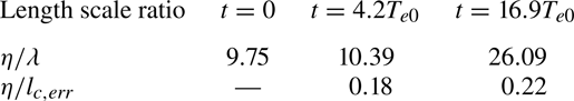
Based on the 2-D cases with varying  $K{{n}_{0}}$, we can further analyse the error growth behaviours across different Reynolds numbers. Based on the error velocity field ${{\boldsymbol {u}}_{error}}$, we define the error kinetic energy as
 \begin{equation} {{K}_{error}}=0.5\langle {{| {{{\boldsymbol{u}}}_{error}}|}^{2}}\rangle. \end{equation}
In figure 13(a), we present the temporal evolution of  ${K}_{error}$ and ${{K}^{th}}$ for 2-D cases with different ${{Re}_{0}}$, where ${{K}^{th}}$ denotes the kinetic energy of thermal fluctuations. It can be observed that ${K}_{error}$ initially equals ${{K}^{th}}$, as the initial error between different flow realizations results solely from thermal fluctuations. As time progresses, ${{K}^{th}}$ increases slowly due to rising temperatures, while ${K}_{error}$ exhibits a more rapid increase compared with ${{K}^{th}}$, reflecting the chaotic nature of turbulent flows. Moreover, as ${{Re}_{0}}$ increases, it becomes apparent that the error growth occurs earlier, leading to a higher ${K}_{error}$. It is noteworthy that a similar trend was observed by Kida et al. (Reference Kida, Yamada and Ohkitani1990), who employed the DNS method to investigate the error growth in 2-D decaying isotropic turbulence.

Figure 13. (a) Displays the temporal evolution of error kinetic energy  $K_{error}$ and thermal fluctuation energy ${{K}^{th}}$ for 2-D cases with different $Re_{0}$, and (b) displays the corresponding results of relative error energy $r={{{K}_{error}}}/{K}$. The $y$-axis of the figure is plotted on a logarithmic scale.
We further calculate the relative error energy  $r$ as the ratio of ${K}_{error}$ to the energy of the original velocity field $K$. The results of $r$ correspond to different $Re_{0}$ are shown in figure 13(b), revealing a similar trend to that of ${K}_{error}$. It is worth noting that, in prior investigations of turbulence predictability, researchers found that the growth of $r$ may conform to the formula $r(t)=r(0)\exp (2{{\lambda }_{Ly}}t)$, where ${{\lambda }_{Ly}}$ is the (effective) Lyapunov exponent (Boffetta et al. Reference Boffetta, Celani, Crisanti and Vulpiani1997). However, we do not observe a clear exponential growth pattern in $r$ from figure 13(b). This is primarily due to the fact that, in our simulations, the initial velocity error due to thermal fluctuations cannot be treated as an infinitesimal perturbation (Boffetta & Musacchio Reference Boffetta and Musacchio2017). Furthermore, considering the relatively low Reynolds number in our current simulations, the phenomenon of exponential growth may not be readily observable (Kida et al. Reference Kida, Yamada and Ohkitani1990).
In figure 14, we conduct a comparative analysis of the energy spectra of the original velocity field  $E$ and the error velocity field $E_{err}$ at $t=27{{T}_{e0}}$ for 2-D cases with different $R{{e}_{0}}$. It is evident that with an increase in $R{{e}_{0}}$, the velocity error propagates more rapidly to larger scales, leading to a closer alignment between $E$ and $E_{err}$ in the low wavenumber range. Moreover, as the increase of $R{{e}_{0}}$, both $E$ and $E_{err}$ show a more distinct inertial range, with their scaling laws approaching the ${{k}^{-3}}{{[\ln (k)]}^{-{1}/{3}}}$ limit, consistent with the Kraichnan-Batchelor-Leith (KBL) theory (Kraichnan Reference Kraichnan1971).

Figure 14. Energy spectra of the original velocity field and the error velocity field at  $t=27T_{e0}$, for the 2-D cases with different $Re_0$.
In addition to the turbulent velocity field, we further investigate the effect of thermal fluctuations on the predictability of the turbulent thermodynamic field, and this aspect has not been reported in the literature. We define the local error fields of the thermodynamic variables as
 \begin{equation} {{g}_{error}}(\boldsymbol{r},t)=\tfrac{1}{\sqrt{2}}({{g}_{1}}(\boldsymbol{r},t)-{{g}_{2}}(\boldsymbol{r},t)), \end{equation}
where  $g$ stands for $T$,
$T$,  $n$ and $P$. Figure 15 presents a comparison between the spectra of the original temperature fields and the error temperature fields for both 2-D and 3-D cases. Similar comparisons can also be made for number density and pressure. At the beginning of USP simulations, the fluctuations of thermodynamic variables are solely attributed to thermal fluctuations, resulting in a complete coincidence between ${{E}_{T}}$ and ${{E}_{T,err}}$. Then, the compressibility of turbulence causes a rapid amplification of ${{E}_{T}}$ to a high magnitude in the low wavenumber region, while ${{E}_{T,err}}$ requires a considerably longer time to approach ${{E}_{T}}$. In figures 16(a,d) and 17(a,d), we present the temperature fields of two realizations during the late stage of turbulence decay for 2-D and 3-D cases, respectively. Compared with the 3-D cases, the differences between the two realizations are more pronounced for the 2-D cases, which can be supported by figure 15(a) where ${{E}_{T,err}}$ almost coincides with ${{E}_{T}}$ at $t=34.6{T}_{e0}$. In figures 16 and 17, we further present the contours of density fields and pressure fields, showing similarities to those of temperature fields.

Figure 15. Spectra of the original temperature field and the error temperature field at different time points, for 2-D case with  $R{{e}_{0}}=1590$ (a) and 3-D case with $R{{e}_{0}}=954$ (b).

Figure 16. Temperature, number density and pressure fields for 2-D decaying turbulence with  $R{{e}_{0}}=1590$ and ${{M}_{t0}}=1$, at $t=34.6{{T}_{e0}}$. Panels (a–c) and (d–f) correspond to two realizations.

Figure 17. Temperature, number density and pressure fields for 3-D decaying turbulence with  $R{{e}_{0}}=954$ and ${{M}_{t0}}=1.2$, at $t=16.9{{T}_{e0}}$. Panels (a–c) and (d–f) correspond to two realizations.
In § 5, we have discussed the coupling relationship between turbulent thermodynamic variables and the compressible velocity component (see figure 9). To see whether this relationship holds for the turbulent error field, we compare the corresponding area-normalized spectra for both 2-D and 3-D cases in figure 18. It is evident that the error spectra of all the thermodynamic variables are in good agreement with the spectrum of the compressible component of the error velocity field. This suggests that in compressible decaying turbulence, the predictabilities of the thermodynamic variables are closely related to the predictability of the compressible velocity component.

Figure 18. (a) Normalized error spectra of compressible velocity component, solenoidal velocity component, temperature, number density and pressure for 2-D decaying turbulence ( $R{{e}_{0}}=954$) at $t=34.6{{T}_{e0}}$. (b) The error spectra corresponding to the 3-D decaying turbulence at $t = 16.9{{T}_{e0}}$.
7. Discussion
In § 5, we employed the USP method to simulate 3-D compressible decaying isotropic turbulence (CDIT) with an initial solenoidal velocity field, focusing on the influence of molecular thermal fluctuations. In recent years, other researchers have examined this case using alternative numerical approaches, with a specific emphasis on the pressure-dilatation behaviours (Cao et al. Reference Cao, Pan and Xu2019; Qi et al. Reference Qi, Chen, Wang, Guo and Chen2022). For instance, Qi et al. (Reference Qi, Chen, Wang, Guo and Chen2022) employed the discrete unified gas-kinetic scheme to simulate CDIT at low and moderate  $M_{t0}$. Based on the time evolution of solenoidal dissipation and pressure-dilatation terms in the TKE equation, they divided the turbulent decaying process into four stages. Furthermore, their findings indicate that the pressure-dilatation transfer occurs more rapidly than the process of vortex stretching and the formation of small-scale vortical structures.
Note that the above works focus on the volume-averaged statistics and do not describe the scale dependence of internal-kinetic energy exchange due to pressure dilatation. To address this issue, Praturi & Girimaji (Reference Praturi and Girimaji2019) numerically studied the effect of pressure dilatation on spectral evolution in CDIT using the GKS. They examined three initial velocity conditions, solenoidal, dilatational and mixed, and their findings indicate that the large-scale dilatational motions exhibit high levels of exchange between internal and kinetic energies due to the pressure-dilatation effect. Furthermore, they found that the high wavenumbers in the dilatational velocity field contain more energy than their solenoidal counterparts. This phenomenon is attributed to the absence of pressure action in enforcing a divergence-free condition, allowing for the formation of shocks. It is worth noting that this phenomenon is also observed in our study, where the compressible (dilatational) velocity spectra  $E_c(k)$ exhibit greater values compared with the solenoidal velocity spectra $E_s(k)$ in the high wavenumber range (see figures 3 and 6). As a consequence, this leads to the cross-over wavenumber of $E_c(k)$ being larger than that of $E_s(k)$ under high $M_{t0}$ conditions.
In the current USP simulations, the initial thermodynamic field exhibits exclusively thermal fluctuations, with no occurrence of large-scale thermodynamic fluctuations. On the other hand, many researchers have previously conducted numerical studies on CDIT with initial thermodynamic fluctuations (Ristorcelli & Blaisdell Reference Ristorcelli and Blaisdell1997; Jaberi, Livescu & Madnia Reference Jaberi, Livescu and Madnia2000; Lee, Yu & Girimaji Reference Lee, Yu and Girimaji2006). Among these works, Lee et al. (Reference Lee, Yu and Girimaji2006) employed the hybrid thermal lattice Boltzmann method to numerically examine CDIT under the influence of large-scale initial temperature fluctuations. They found that the overall effect of pressure dilatation is to transfer energy from thermal to kinetic modes at large scales. The transferred kinetic energy is manifested as the dilatational velocity field, with subsequent cascading of large-scale dilatational fluctuations towards smaller scales.
In this study, large-scale temperature fluctuations primarily result from the compressibility of turbulence. Our numerical findings indicate that the spatial correlation of temperature fluctuations is dominated by the compressible mode of the velocity field (see figure 9). On the other hand, for incompressible turbulent flows, previous researchers have studied temperature fluctuations arising from dissipation rate fluctuations (Bos, Chahine & Pushkarev Reference Bos, Chahine and Pushkarev2015; Pushkarev, Balarac & Bos Reference Pushkarev, Balarac and Bos2017). In this context, temperature is modelled as a passive scalar, and existing literature results demonstrate a strong dependence of the wavenumber scaling of the temperature spectrum on the scaling of the dissipation rate spectrum (Bos et al. Reference Bos, Chahine and Pushkarev2015). The USP method employed in our study can be directly applied to this scenario, allowing for further investigation into the impact of thermal fluctuations.
8. Concluding remarks
In this work, we employed the USP method to numerically investigate the effects of thermal fluctuations on CDIT. Compared with the traditional molecular methods such as DSMC, USP can be applied with much larger time steps and cell sizes as it couples the effects of molecular movements and collisions.
In both 2-D and 3-D simulations, it is found that the turbulent spectra of velocity and thermodynamic variables are greatly affected by thermal fluctuations in the high wavenumber range. The wavenumber scaling law of the thermal fluctuation spectra depends on the spatial dimension  $d$ as ${{k}^{(d-1)}}$. By applying the Helmholtz decomposition to the velocity field, we show that the thermal fluctuation spectra of solenoidal and compressible velocity components (i.e. ${{E}_{s}}(k)$ and ${{E}_{c}}(k)$) follow an energy ratio of 1 : 1 for 2-D cases, while this ratio changes to 2 : 1 for 3-D cases.
For 3-D decaying turbulence, a comparative study was conducted between the USP method and the DNS method based on the deterministic NS equations. The results show that thermal fluctuations dominate the turbulent spectra below length scales (i.e. the cross-over length scales) comparable to the Kolmogorov length scale  $\eta$, which shows good agreement with the previous studies (Bell et al. Reference Bell, Nonaka, Garcia and Eyink2022; McMullen et al. Reference McMullen, Krygier, Torczynski and Gallis2022b). Furthermore, it is observed that the cross-over wavenumbers of thermodynamic spectra increase with ${M}_{t}$ following a similar trend as the cross-over wavenumber of ${{E}_{c}}(k)$, indicating the coupling relationship between thermodynamic fluctuations and the compressible mode of the velocity field.
In addition to the turbulent spectra, our results demonstrate that thermal fluctuations also play an important role in the predictability of turbulence. Specifically, with initial differences attributed solely to thermal fluctuations, different flow realizations exhibit large-scale divergences in velocity and thermodynamic fields after a certain period of time. By calculating the error spectra between flow realizations, our study reveals the ‘inverse error cascades’ for velocity and thermodynamic variables. Moreover, our results suggest a strong correlation between the predictabilities of thermodynamic variables and the predictability of the compressible velocity component.
In this study, we focused on the effects of thermal fluctuations on homogeneous isotropic turbulence, but we expect thermal fluctuations to be important for other turbulent flow scenarios, such as laminar–turbulent transition (Luchini Reference Luchini2016) and turbulent mixing (Eyink & Jafari Reference Eyink and Jafari2022). In the latter case where molecular diffusion becomes significant, there is a need to extend the kinetic models that form the basis of USP for precise determination of gas diffusion coefficients (Todorova & Steijl Reference Todorova and Steijl2019). For the predictability of turbulence, further research is required to investigate the error growth behaviours across a wider range of Reynolds numbers, along with a detailed comparative analysis between 2-D and 3-D cases.
Acknowledgements
The authors thank Professor F. Fei, Dr C. Zhao and Professor J. Wang's group for helpful discussions about this work. The authors also thank Professor L. Pan for providing the GKS code for 2-D turbulence simulations.
Funding
This work was supported by the National Natural Science Foundation of China (grant nos. 92052104, 92371102 and 12272028). Part of the results were obtained on the Zhejiang Super Cloud Computing Center Zone M6, and others were obtained on the Beijing Super Cloud Computing Center Zone A.
Declaration of interests
The authors report no conflict of interest.


