


1. Introduction
An increase in the demand for micro air vehicles has resulted in greater interest in how wings operate within turbulent environments at moderately low Reynolds numbers. Applications of micro air vehicles include flight missions within large cities where the turbulence intensities are typically 10 %–20 % at length scales of up to 10 times the order of magnitude of the aircraft's chord (Roth Reference Roth2000). The first investigation into the effect of free-stream turbulence (FST) on airfoil characteristics was completed by Hoffmann (Reference Hoffmann1991). The benchmark study investigated how FST affects the lift, drag and surface flow on a NACA0015 airfoil. Hoffmann (Reference Hoffmann1991) observed that at the highest level of FST (9 %), the peak lift coefficient increased by 30 %, and the onset of stall was delayed by  $5^\circ$. As the FST varied, the maximum drag coefficient remained constant. Similar investigations conducted into the effect of FST are outlined in table 1, highlighting a lack of quantitative investigation into the flow field surrounding a wing subject to incoming FST where the length scale is decoupled from the turbulence intensity.
Table 1. Summary of previous investigations into the response of a rigid wing subject to FST. Note: F, forces and moments; FV, flow visualisation; SP, surface pressure; PIV, particle image velocimetry;  $\prime$, fluctuations. Here, $\Uparrow$ denotes an increase, $\Downarrow$ denotes a decrease and $\approx$ denotes no observed change.

Investigations such as those by Hoffmann (Reference Hoffmann1991), Yap et al. (Reference Yap, Abdullah, Husain, Ripin and Ahmad2001) and Cao, Ting & Carriveau (Reference Cao, Ting and Carriveau2011) use a load cell to measure the total force produced by a wing. These investigations observe an average increase in the peak lift coefficient of 34 %. In contrast, investigations such as those by Kay, Richards & Sharma (Reference Kay, Richards and Sharma2020) and Ravi et al. (Reference Ravi, Watkins, Watmuff, Massey, Peterson and Marino2012) use pressure measurements on the wing's surface to determine the lift. These investigations calculate an average increase in the peak lift coefficient of 7.5 %. This large disparity between the sectional and total increase in lift coefficient suggests that there is a three-dimensional suppression by the introduction of FST, which is not accounted for when measuring the wing sectionally.
Work by Cao et al. (Reference Cao, Ting and Carriveau2011), Ravi et al. (Reference Ravi, Watkins, Watmuff, Massey, Peterson and Marino2012) and Vita et al. (Reference Vita, Hemida, Andrianne and Baniotopoulos2020) set out to determine the effect of the integral length scale of incoming turbulence on a wing. Cao et al. (Reference Cao, Ting and Carriveau2011) investigated the time-averaged lift and drag of a  $S1223$ wind turbine blade. The results showed that increasing the integral length scale increased the time-averaged lift and drag. This increase was observed to be greater at lower turbulence intensities. Vita et al. (Reference Vita, Hemida, Andrianne and Baniotopoulos2020) investigated a $DU96w180$ wind turbine airfoil. Using pressure taps, the study investigated the time-averaged mean and standard deviation of the surface pressure of the wing. The study found that at normalised integral length scales less than 1, the effect of turbulence is weaker and the magnitude of the standard deviation is amplified for integral length scales equal to the chord. Ravi et al. (Reference Ravi, Watkins, Watmuff, Massey, Peterson and Marino2012) investigated how variations in integral length scale affect a thin airfoil. Similar to work by Cao et al. (Reference Cao, Ting and Carriveau2011), Ravi et al. (Reference Ravi, Watkins, Watmuff, Massey, Peterson and Marino2012) found that increasing the integral length scales causes an increase in the time-averaged peak lift coefficient. Using pressure taps, Ravi et al. (Reference Ravi, Watkins, Watmuff, Massey, Peterson and Marino2012) observed that at integral length scales greater than the chord, the magnitude of the standard deviations is larger than when the integral length scale is equal to the chord. The discrepancies in the findings of Ravi et al. (Reference Ravi, Watkins, Watmuff, Massey, Peterson and Marino2012) and Vita et al. (Reference Vita, Hemida, Andrianne and Baniotopoulos2020) may be a result of the differing airfoil geometries. Moreover, Kay et al. (Reference Kay, Richards and Sharma2020) suggest that airfoil geometry, namely camber, plays a significant role in the effect of FST on a wing.
From the above discussion, it is clear that the physics underlying the effects of varying the integral length scale of incoming FST on the performance of a wing remains unknown. Moreover, these effects have been discussed in previous work only in terms of the time-averaged mean and standard deviation of pressure and forces. Very little information is available on the spectral content of force and moment fluctuations experienced by wings in the presence of FST. Furthermore, there is a lack of quantitative investigation into the flow field surrounding a wing subject to FST. In this study, we aim to address these gaps in the literature by exploring the effects of the integral length scale of FST on the performance of a wing. We focus on high FST ( $\approx$15 %) and vary the integral length scale of the turbulence from 0.5 $c$ to 1 $c$. Particular attention is paid to understanding the changes in force and moment fluctuations of the response of a rigid wing and how the surrounding flow field induces those fluctuations.
2. Experimental methods
2.1. Turbulence generation
All experiments are conducted within the University of Southampton's ‘Göttingen’-type closed wind tunnel with a closed test section. Each test segment has an internal width of 1.2 m, an internal height of 1 m and a length of 2.4 m. The tunnel is equipped with a ‘cooling unit’ comprising two heat exchangers and a temperature controller such that the air temperature remains constant within the test section. In the clean configuration, the free stream has a turbulence intensity of less than 0.1 %.
To generate the required FST, a custom-built Makita-style active grid is developed. The grid features 11 horizontal shafts and 13 vertical shafts, with a total of 172 winglets with a grid spacing of  $M = 0.085$ m. Each shaft is able to spin to 2000 r.p.m. The grid is capable of achieving a winglet closed area ratio (WCAR) of range 0.7–1 by using different winglet geometries. The active grid operates in a double random mode, shown by Poorte & Biesheuvel (Reference Poorte and Biesheuvel2002), where the velocity and operational time of each shaft are chosen based on specified random intervals. The width and method of random choice of those intervals are known to have a large effect on the resulting turbulence spectra, as shown by Hearst & Lavoie (Reference Hearst and Lavoie2015). Preliminary investigations determined that the interval for the operational time is 0.05 to 5 s and the angular velocity $\omega$ has a range of $\pm$50 % with a top-hat distribution. This ensures that the generated turbulence spectra do not include a unique frequency in the production range, as seen in figure 1 by a constant spectral content in the lower frequencies. By changing the WCAR and angular velocity, the turbulence intensity is kept approximately constant whilst varying the integral length scale, as seen in table 2.

Figure 1. (a) Spectral content of turbulent cases from hot-wire anemometry (HWA). The angled dashed line represents Kolmogorov's  $-5/3$ law. (b) The streamwise autocorrelation coefficient from PIV where $\delta$ is the spatial lag. The horizontal solid line represents the correlation threshold.
Table 2. Turbulence generation parameters and turbulence characteristics of the four cases investigated using HWA and PIV.

A single-wire probe with a  $5\ \mathrm {\mu }{\rm m}$ tungsten wire is used to characterise the flow generated by the active grid. The probe is operated using a Dantec 54N80 Multichannel CTA with an overheat factor of 0.8. The system is optimised to ensure a flat frequency response at 10 kHz. Following a sampling and convergence study, an acquisition rate of 25 kHz for 180 s is used, where all signals are subject to a low-pass filter at 10 kHz. For data acquisition, a NI DAQ 6251 M series is used. The probes are calibrated before and after each measurement using a Pitot static probe placed close to the hot wire connected to a FCO510 micromanometer. The calibration curve used is a King's law curve. The micromanometer is connected to the NI DAQ, sampling at 5 kHz.
Four turbulent cases are evaluated within this investigation at  $Re=2\times 10^5$, such that the integral length scale can be independently changed. The turbulence generated is evaluated using the above-mentioned single-wire method at a point located in the centre of the tunnel at the airfoil's quarter chord. The generated turbulence is also evaluated by means of a spanwise planar PIV experiment. For both the PIV and the hot-wire method, the turbulence intensity is determined as $T_u = U_{rms}/U_{mean}$ where $U_{rms}$ is the root mean square of the velocity and $U_{mean}$ is the mean velocity. For the hot-wire method the integral length scale $L_x=U_\infty T_l$ is determined via integration of the zero-crossing point of the autocorrelation
 \begin{equation} T_l = \int_{0}^{\infty} \rho_x (\tau) \,{\rm d}t , \end{equation}
where  $\tau$ is the time lag and $\rho _x$ is the autocorrelation coefficient, defined as
 \begin{equation} \rho_x (\tau) = \frac{R_x(\tau)}{R_x(0)} , \end{equation}
where  $R_x$ is the autocorrelation function in time. Work by Mora & Obligado (Reference Mora and Obligado2020) finds that the autocorrelation function generated by active-grid flows may exhibit a non-decaying behaviour. However, in the current study the autocorrelation is found to decay to zero in a timely manner, so a zero-crossing approach is applicable. Figure 1 shows that for the PIV method the autocorrelation did not decay to zero. Consequently, the length scale was determined based on a threshold of the autocorrelation equal to 0.2, shown by the solid black line in figure 1. This threshold is arbitrary and leads to an increase in the length scale as lower threshold values are used. Despite this, our selection of this specific threshold value was guided by its ability to yield the most accurate agreement with the length scale obtained from hot-wire data. Furthermore, the analysis revealed three distinct length scales irrespective of the threshold chosen. The turbulence characterisation results are presented in table 2, indicating a maximum difference of 5 % and 20 % for the turbulence intensity and integral length scale, respectively, between the hot-wire and PIV methods. Such variations are anticipated in flows of this nature. Throughout the remaining sections of the paper the turbulent cases will be referenced by $({L_x/c})_{approx}$, which is approximated from the HWA. The generated turbulence has an anisotropy ratio of $u^{\prime }/{v^{\prime }}=1.3\pm 0.2$, expected from convective flows of this nature.
2.2. Forces and moments
The rectangular wing has a NACA0012 profile, 0.75 m span and 0.3 m chord with no flow-tripping devices applied to the wing's surface. The wing comprises three aluminium spars wrapped in carbon fibre to ensure rigidity. The wing is mounted to the ceiling of the tunnel test section, such that the quarter chord is 1.8 m (21M) downstream of the active grid. The distance to the grid is closer than the more commonly used 40M; however, from volumetric hot-wire and planar PIV analyses, the grid is observed to produce homogeneous turbulence in the horizontal direction ( $y$-axis) for all cases, with variations of less than $\pm$2.5 % for the mean flow and turbulence statistics. A stepper motor is connected to the root of the wing, allowing for a $360^\circ$ range of motion. A 6-axis ATI IP15 SI165 load cell is placed at the root of the stepper motor to determine the forces and moments exerted by the wing. The measurement uncertainty at a 95 % confidence level as a percentage of full-scale load is 1.25 %. Following a preliminary impulse experiment, the natural frequency of the system is 11.7 Hz. Figure 2 shows the stepper motor and load cell protruding outside the test section through transparent acrylic such that there are no additional aerodynamic effects from any part of the system. A flow splitter is mounted within the test section 1 mm from the wing tip to ensure suppression of the wing tip vortex. For all cases, the angle of attack is stepped from 0 to $20^\circ$ in increments of $1^\circ$. Following a sampling and convergence study, data are acquired at 1 kHz for 120 s at each angle. As a result of the three-dimensional nature of the wing and the location of the load cell, the forces observed are integrated across the wingspan and therefore the statistics interpreted by the load cell are filtered by the wing itself.

Figure 2. Schematic representation of the PIV set-up. The green areas represent laser sheets, the blue and orange dashed lines represent the field of view of each camera, the grey rectangle represents the flow splitter and the grey cylinder represents the 6-axis load cell.
2.3. Particle image velocimetry
Figure 2 shows the planar PIV set-up used to investigate the flow field surrounding the NACA0012 wing in the four aforementioned turbulence conditions at an angle of attack of  $16^\circ$ at $Re=2\times 10^5$. Preliminary investigations indicate a spanwise homogeneity of the incoming turbulent flow. With the use of tell tales it is observed that the production of three-dimensional flow features (stall cells) are not evident with the introduction of FST. Hence, with a statistically converged number of snapshots, planar PIV at any spanwise location (away from the boundaries) gives a two-dimensional statistical understanding of the flow field.
Two Nd:YAG Bernoulli lasers manufactured by Litron are used to illuminate both the suction and the pressure sides of the wing in the chordwise plane, a full chord from the wing tip. The lasers are positioned to ensure full coverage of the surrounding flow field. The lasers emit a double pulse of monochromatic light shaped by mirrors and a cylindrical lens to form a light sheet 2 mm thick. Mounted above the wing are two LaVision ImagerProLX cameras. The cameras are equipped with macro lenses of 50 mm focal length. The distance between the cameras and the illuminated region provides a field of view of  $475\ {\rm mm} \times 800\ {\rm mm}$ surrounding the airfoil, resulting in a resolution of 9.9 pixels per millimetre. The trade-off to ensure a large field of view capable of capturing the wing's wake comes at the expense of a more resolved boundary region. Work by Istvan & Yarusevych (Reference Istvan and Yarusevych2018) and Yarusevych & Kotsonis (Reference Yarusevych and Kotsonis2017) concluded that a bypass transition effectively eliminates the laminar separation bubble at high turbulence intensities. Therefore, it is beneficial to explore an extended field of view that has not been previously measured.
The cameras and lasers are controlled by the PIV system developed by LaVision, which is implemented in the software DaVis 8.4. The software manages the data acquisition, storage and timing of the triggers to the laser and cameras. A desktop computer with an inbuilt programmable timing unit manufactured by LaVision is used to ensure the relative timing of these signals. For each turbulence case 2500 image pairs are captured at 0.6 Hz, and for each clean case 1000 image pairs are captured at 0.6 Hz. A channel of the data acquisition system used to measure the force and moments from the load cell is connected to the laser trigger, such that the timings of the acquired images can be concurrently matched to the resulting forces and moments produced by the wing. The forces and moments are sampled at 10 kHz for the duration of the PIV case to ensure that each image trigger is captured.
An image pre-processing method described by Mendez et al. (Reference Mendez, Raiola, Masullo, Discetti, Ianiro, Theunissen and Buchlin2017) is implemented whereby proper orthogonal decomposition is used to determine the modes of a set of raw images. The first modes chosen with the given tolerances  $\epsilon _1=0.01$ and $\epsilon _2=0.01$ are subtracted from the raw images, which can be thought of as a background and noise subtraction. The images are processed with an in-house MATLAB script, resulting in a vector field that has a spatial resolution of one vector every 0.78 mm using a final interrogation window of $32\times 32$ pixels.
3. Results
3.1. Forces and moments
With a clean inflow, the NACA0012 wing stalls at an angle of attack of  $10^\circ$, as shown in figure 3 by a decrease in lift, increase in drag and reduction in pitching moment. Similar to previous literature, the introduction of FST causes the onset of stall to be delayed. The angle of maximum lift for the turbulent cases is observed to be between 16 and $17^{\circ }$ with a peak lift coefficient 40 % larger than that of the clean inflow case. The large increase in peak lift coefficient is consistent with previous investigations by Hoffmann (Reference Hoffmann1991), Yap et al. (Reference Yap, Abdullah, Husain, Ripin and Ahmad2001) and Cao et al. (Reference Cao, Ting and Carriveau2011), who observed increases of 30 %, 38 % and 33 %, respectively. Generally, the time-averaged forces and moments of the wing subject to FST are similar. An increase in the length scale is observed to cause a 5 % increase in the peak lift coefficient obtained by the rigid wing, echoing results found by Ravi et al. (Reference Ravi, Watkins, Watmuff, Massey, Peterson and Marino2012) and Cao et al. (Reference Cao, Ting and Carriveau2011). The time-averaged drag of the turbulent cases remains relatively similar. The time-averaged pitching moment of the turbulent case where $L_x/c\approx$ 0.5 shows a slightly shallower gradient as the wing begins to stall. This agrees with the results of Ravi et al. (Reference Ravi, Watkins, Watmuff, Massey, Peterson and Marino2012) in that a reduction in integral length scale is found to reduce the gradient of the time-averaged pitching moment for turbulence intensities of 7 % and 12 %. This shallower gradient suggests that the flow over the wing stays more attached, as the wing is acting less like a bluff body than in the other turbulent cases.

Figure 3. (a–c) Time-averaged mean and (d–f) standard deviation of the (a,d) lift, (b,e) drag and (c,f) pitching moment coefficient against the angle of attack. The dashed line in the time-averaged lift represents thin airfoil theory.
Figure 3 shows that the standard deviation of the clean flow measurements increases as stall occurs, and then decreases as the wing begins to act as a bluff body. With the introduction of FST, the standard deviations of the measurements increase as a result of the fluctuating inflow. The standard deviation of the lift coefficient for the case of  $L_x/c\approx 0.5$ is nearly 50 % larger than that of the other turbulent cases, and remains constant for all turbulent cases at angles of attack below $10^\circ$. Above this threshold, the standard deviations increase with angle of attack. Observing the standard deviation of the drag coefficient, the three turbulent cases are similar for angles of attack below $10^\circ$, with a slight reduction in the $L_x/c\approx 1.0$ case for angles less than $6^\circ$. However, for angles of attack greater than $10^\circ$, the case of $L_x/c\approx$ 0.5 shows a dramatic increase of 80 % compared with the cases of $L_x/c\approx 0.7$ and $L_x/c\approx$ 1.0. The standard deviations of the pitching moment are similar to those of the lift coefficient, with a 65 % increase in standard deviation of the $L_x/c\approx 0.5$ case compared with the other turbulent cases. Figure 3 displays an obvious increase in fluctuations across the lift, drag and pitching moment for a normalised integral length scale of $L_x/c\approx 0.5$. This phenomenon could be attributed to the fact that as the length scale reduces, the wing experiences a larger occurrence of events with the same energy, and hence there is an observed increase in measured fluctuations.
Spectral analysis is conducted to better understand the distribution of force and moment fluctuations resulting from different integral length scales. Figure 4 displays the normalised power spectral density of the lift and drag coefficients. There is an observed increase in power with the addition of FST by an order of magnitude, resulting from the higher energy within the flow. There is also the introduction of a broad range of spectral content over all angles of attack for the lift, with a greater magnitude observed at angles larger than  $15^\circ$. Similarly, for the drag, a broad range of spectral content is shown, but only for angles larger than $15^\circ$. Investigations by Li & Hearst (Reference Li and Hearst2021) and Kay et al. (Reference Kay, Richards and Sharma2020) comparably observe an order-of-magnitude increase with the introduction of FST. Moreover, the presence of a broad range of spectral content is observed over all angles of attack. For the $L_x/c\approx 0.5$ case there is an increase in the peak power of over 90 % in the lift and 250 % in the drag compared with the case where $L_x/c\approx 1.0$. In the clean inflow case, the location of maximum power is highlighted at a reduced frequency of $k_{clean} = fc/2U_\infty = 0.18$ by the horizontal dashed black line. This is the natural response of the system, and a spectral peak at this frequency is observed for all flow conditions. For each turbulent case, the system's natural reduced frequency is made equivalent to the Strouhal number of the incoming turbulence, $k_{turb}= fL_x/U_\infty$. Each calculated reduced frequency is marked with a black dotted line at 0.18, 0.13 and 0.09 for $L_x/c\approx 0.5$, 0.7 and 1.0, respectively. It is observed that for the $L_x/c\approx 0.7$ and $L_x/c\approx 1.0$ cases there is an increase in power below the marked line as a direct result of the fluctuations of the incoming flow. Those cases also demonstrate a marginal amplification of the fluctuations above those lines. For the $L_x/c\approx 0.5$ case, the reduced frequency based on the integral length scale coincides with the natural response of the separated flow, suggesting a superposition between the system and the turbulent flow, which presumably leads to more intense fluctuations.

Figure 4. Normalised power spectral density of the measured (a–d) lift and (e–h) drag for angle of attack against reduced frequency. For the clean inflow case the peak is marked. For the turbulent cases  $fL_x/U_\infty$ is marked with a dashed line.
3.2. Particle image velocimetry
The turbulent flow fields surrounding the wing are measured using planar PIV to understand the phenomena of the increased fluctuations and spectral amplitude. Figure 5 illustrates the streamwise component of the mean velocity field (filled contours) and turbulence intensity (contour lines) for each inflow case. The PIV was conducted at an angle of attack of  $\alpha = 16^{\circ }$, as this was not only the maximum lift angle of the turbulent cases but also the angle of attack at which the drag coefficient of the clean and turbulent cases coincide. The mean velocity field of the clean inflow case displays a fully separated flow with separation occurring at the leading edge. A recirculation region is present as indicated by the blue contours, which denote reversed flow. The introduction of FST appears to suppress the recirculation region, allowing the flow to remain more attached to the wing, hence the larger lift coefficient and delayed stall. Flow reversal is observed very close to the wing's surface for all FST cases, resulting from the adverse pressure gradient present. However, the small separation bubble does not extend into the wake of the wing. The mean velocity fields of the three turbulent cases are very similar, as expected from the similarity in time-averaged force and moment coefficients, with a slight discrepancy in the size of the wake. For the $L_x/c\approx 0.5$ case, the wake region is the smallest of the turbulent cases and the flow appears most attached, which is expected from the observations of the shallower gradient of the pitching moment. For the turbulent case of $L_x/c\approx 0.7$, the wake is longer and slightly wider than that of the $L_x/c\approx 0.5$ case, indicated by the $T_u=0.8$ contour reaching the edge of the PIV domain. For the $L_x/c\approx 1.0$ case, the wake region is again slightly larger than that of the $L_x/c\approx 0.7$ case, shown by the widening contours of turbulence intensity. Aside from the slightly larger wake regions, the turbulent mean fields are otherwise very similar.

Figure 5. Time-averaged streamwise velocity of a NACA0012 wing at  $\alpha =16^\circ$ with contour lines showing $T_u$.
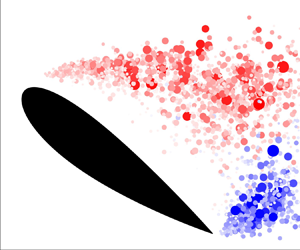
The similarity of the time-averaged flow fields explains the results of the time-averaged forces, but it does not explain the differences in the fluctuations of said forces. To better understand the causes of these fluctuations, vortex identification is used. Figure 6 represents the location, size and strength of vortices detected in the instantaneous flow fields. The vortex centre is identified using the  $\varGamma _{1}$ criterion and the vortex area is identified using the $\varGamma _{2}$ criterion outlined by Graftieaux, Michard & Grosjean (Reference Graftieaux, Michard and Grosjean2001). To avoid measurement-related over-sampling $N=11$ is used, where $N$ is a spatial filter, removing the small-scale fluctuations that could stem from PIV noise. For the clean inflow case, distinct leading- and trailing-edge vortices are observed. The two types of vortices nucleate from single locations and convect downstream towards the wake of the wing, leaving no apparent vortices within the separated boundary layer. With the introduction of FST, there are no longer two distinct nucleation locations for the generation of vortices. Clockwise vortices appear along the entire suction side of the wing, with a larger dispersion area as they convect downstream. The trailing-edge vortices are suppressed, with lower size, strength and quantity. For the $L_x/c\approx 0.5$ case the vortices are closer to the wing's surface than in the other turbulent cases. For the $L_x/c\approx 0.7$ and $L_x/c\approx 1.0$ cases, the generated vortices are convected and dispersed over a larger area. This dispersion of vortices accounts for the larger wake observed in the mean flow for the cases of $L_x/c\approx 0.7$ and $L_x/c\approx 1.0$.

Figure 6. Location, size and strength of the vortices in the flow field around a NACA0012 wing at  $\alpha =16^\circ$. The size of the circles represents vortex area and the colour represents normalised circulation.
Figure 6 displays only a qualitative overview of the instantaneous vortices captured; therefore, to appropriately compare the four cases, a quantitative analysis is carried out. Figure 7 shows the joint probability density function of the normalised vortex circulation and size for all four cases. The assumption that the vortices are circular is used to determine the vortex diameter, denoted by  $d$. For the clean flow case, the majority of vortices have a normalised diameter of $d/c=0.08$ and normalised circulation of $\varGamma /U_\infty c=0.006$ with a positive correlation. When introducing FST with $L_x/c\approx 0.5$, there appears to be little change in the probability density function. The peak magnitude of the probability density function differs by only 2 % from the clean inflow case. The similarities between the vortices generated by the clean and $L_x/c\approx 0.5$ cases could explain why the spectral peaks of the forces are the same. However, as there is more energy in the $L_x/c\approx 0.5$ case due to the turbulence, the magnitude of the spectral peak is larger. When introducing FST with $L_x/c\approx 0.7$, there is a slightly larger spread in the probability density function for larger, stronger vortices. The location of the peak of the density function is consistent with the other cases; however, there is a reduced peak magnitude of 15 % compared with the $L_x/c\approx 0.5$ case. The reduced peak magnitude and broader range of the density function explains why the force spectra of the $L_x/c\approx 0.7$ case display a broader range of power over different frequencies. For the case where $L_x/c\approx 1.0$, there is an even greater spread in the probability function for larger, stronger vortices, and the peak is over 25 % less than that of the $L_x/c\approx 0.5$ case. This is consistent with the lower power and broader range of frequencies observed in the force spectra.

Figure 7. Joint probability density function of vortex strength and size for (a) the clean inflow case and the turbulent cases of (b)  $L_x \approx 0.5$, (c) $L_x \approx 0.7$ and (d) $L_x \approx 1.0$.
4. Conclusion
This study has investigated the effect of variations in integral length scale of incoming FST on the response of a rigid NACA0012 wing. Forces, moments and the flow field were measured using a force sensor and planar PIV. The addition of FST was found to increase the time-averaged lift coefficient whilst delaying the onset of stall. It was observed that the flow remained attached with the introduction of FST compared with that of clean inflow and there was a complete suppression of the recirculation bubble. With a turbulent inflow there was an increase in the production of vortices along the suction side of the wing, whilst there was a decrease in the production of trailing-edge vortices.
It was found that variations in the integral length scale of incoming turbulence greatly affect the fluctuating response of a rigid wing. At integral length scales equivalent to half of the chord of the wing, there was an increase in the standard deviation of the forces and moments. It was observed at this length scale that the flow is attached with a smaller wake. Vortical structures appeared to stay closer to the wing's surface and have a more distinct characteristic strength and size. In contrast, at larger integral length scales there was a spread of the size and strength of vortices generated by the wing, resulting in a broader range of force spectra. Comparing this study with previous work confirms that airfoil geometry and turbulence-generation techniques are parameters that highly affect the response of a wing to variations in integral length scale.
Funding
We gratefully acknowledge funding from EPSRC (grant ref. EP/V05614X/1) and the School of Engineering at the University of Southampton for C.T.'s PhD studentship.
Declaration of interests
The authors declare no conflict of interest.
Data availability statement
All data supporting this study are openly available from the University of Southampton repository at https://doi.org/10.5258/SOTON/D2792.
Author contributions
C.T. designed the experiment, carried out measurements, analysed the data and wrote the first draft. H.B. contributed to some analysis, the editing of several drafts and carrying out the measurements. S.S. supervised the work and edited several drafts. B.G. was responsible for conceptualisation, funding acquisition, the editing of drafts and project management.


 Open access