


1. Introduction
The thermally driven flow inside a fluid layer heated from below and cooled from above, known as Rayleigh–Bénard convection, is a widely studied physical problem due to its similarities with a range of real-life applications and physical phenomena. Despite its apparent simplicity, this type of convection exhibits rich physics in terms of both large-scale characteristics (e.g. Nusselt number and large-scale circulation; see the review by Ahlers, Grossmann & Lohse Reference Ahlers, Grossmann and Lohse2009) and small-scale turbulence dynamics (e.g. spectra and structure functions; see Lohse & Xia Reference Lohse and Xia2010). Even in its simplest form, the complexity of the flow increases rapidly with the Rayleigh number, with progressively thinner boundary layers and smaller thermal plumes. Consequently, resolving these smaller structures in numerical simulations imposes overwhelming resolution requirements (Shishkina et al. Reference Shishkina, Stevens, Grossmann and Lohse2010). Moreover, when additional complexities are included in the configuration, such as solid particles suspended in the fluid phase (Demou et al. Reference Demou, Ardekani, Mirbod and Brandt2022) or two fluid layers (Liu et al. Reference Liu, Chong, Yang, Verzicco and Lohse2022), the numerical solution becomes even more challenging.
Focusing on thermal convection between two fluid layers, the need to study this specific problem stems from the fact that, regardless of the application, there is always some dissolved gas in every liquid. Therefore, it is almost inevitable that a gaseous phase will be formed in any realistic natural convection flow. This is also evident in experiments on natural convection in liquids, where a long degassing procedure should be followed to prevent the formation of the gaseous phase: (i) the liquid phase is heated close to boiling point, (ii) a pump sucks the released gas, and (iii) the treated liquid must be kept isolated to prevent any gases from dissolving back into the liquid. The proposed study aims to facilitate the transition from the ideal problem to a more realistic set-up by considering the gaseous phase in a two-layer configuration. From an application point of view, physical phenomena such as the convection in the Earth's mantle (Busse Reference Busse1981), or engineering applications such as the heat transfer inside magnetic confinement systems in fusion reactors (Wilczynski & Hughes Reference Wilczynski and Hughes2019), are more accurately modelled as a two-layer convection, where the two fluid layers are dynamically coupled.
Before introducing the two-layer Rayleigh–Bénard convection, it is vital to understand some key characteristics of the classical Rayleigh–Bénard convection in a single fluid. This problem is determined by three control parameters: the Rayleigh number ( $Ra$), the Prandtl number ( $Pr$), and the aspect ratio ( $\varGamma$) of the cavity within which the thermal convection takes place. The dependence of all physical features (including flow regime, flow structures and heat transfer) on only three control parameters is partly due to adopting the Oberbeck–Boussinesq approximation (Oberbeck Reference Oberbeck1879; Boussinesq Reference Boussinesq1903), which, in brief, assumes constant fluid properties except for the density in the gravitational term, which varies linearly with the temperature. Within this physical setting, the Grossmann–Lohse theory (Grossmann & Lohse Reference Grossmann and Lohse2000; Stevens et al. Reference Stevens, van der Poel, Grossmann and Lohse2013) provides scaling laws for the Reynolds number ( $Re$) and Nusselt number ( $Nu$) with respect to the control parameters, assuming different exponent values in different $Ra$–
$Ra$– $Pr$ regimes. This theory is based on the existence of a coherent large-scale convection roll, something that is not necessarily true in the two-layer configuration where each layer develops its own confined convection rolls, which can be qualitatively very different.
Moving on to the two-layer Rayleigh–Bénard configuration, new control parameters should be considered, even within the limits of applicability of the Oberbeck–Boussinesq approximation. First, each layer is composed of a different fluid with constant thermophysical properties. Hence the ratios of density, viscosity, conductivity, thermal expansion and heat capacity also become governing parameters. In addition, since the two layers are separated by a deformable interface featuring surface tension, the Weber number ( $We$) should also be considered. Furthermore, the Froude number ( $Fr$) is included to differentiate between the relative effects of gravity in the two fluids. This set of control parameters is translated into an enhanced flow complexity with many different regimes depending on the combination of these parameters (Liu et al. Reference Liu, Chong, Wang, Ng, Verzicco and Lohse2021).
While experimental studies of two-layer Rayleigh–Bénard convection have been conducted for a few decades now (Zeren & Reynolds Reference Zeren and Reynolds1972; Degen, Colovas & Andereck Reference Degen, Colovas and Andereck1998; Xie & Xia Reference Xie and Xia2013), direct numerical simulations (DNS) studies appeared in the literature only recently. In a series of publications, Yoshida and co-workers utilized DNS to study two-layer Rayleigh–Bénard convection in a two-dimensional spherical shell geometry (Yoshida & Hamano Reference Yoshida and Hamano2016; Yoshida et al. Reference Yoshida, Iwamori, Hamano and Suetsugu2017; Yoshida Reference Yoshida2019). By considering large viscosity differences between the two fluids, these authors focused on characterizing the large-scale flow structures in each fluid, and the dynamic coupling of these structures through the interface. Most recently, Liu et al. conducted DNS in two-dimensional (Liu et al. Reference Liu, Chong, Wang, Ng, Verzicco and Lohse2021) and three-dimensional (Liu et al. Reference Liu, Chong, Yang, Verzicco and Lohse2022) rectangular cavities. In their two-dimensional study, these authors considered a wide range of Weber numbers and density ratios, identifying two qualitatively different mechanisms of interface breakup based on these two parameters. In their three-dimensional study, they focused on the effects of the relative thickness of each layer and the thermal conductivity ratio, suggesting a model to predict the interface temperature and the global heat transfer within the explored parameter space. Finally, Scapin, Demou and Brandt (Reference Scapin, Demou and Brandt2023) moved even further and included evaporation along the two-fluid interface, extending the model proposed in (Liu et al. Reference Liu, Chong, Yang, Verzicco and Lohse2022) to account for non-Oberbeck–Boussinesq effects and evaporation.
Even though the aforementioned works contributed to the understanding of several aspects of two-layer Rayleigh–Bénard convection, important open questions still need to be addressed. First, the influence of the Rayleigh and Weber numbers on the movement of the interface remains elusive. While Liu et al. (Reference Liu, Chong, Wang, Ng, Verzicco and Lohse2021) thoroughly described the scenarios under which the interface breaks for different Weber numbers and density ratios, the interface oscillation modes well before breakup were not characterized. Additionally, further insight into the temperature distribution and variations of quantities, such as the thermal boundary layer thickness and the interface temperature, is necessary for a deeper understanding of the heat transfer near the interface. More specifically, the extent to which the top and bottom thermal boundary layers are affected by the asymmetrical two-layer structure considered here, is one of the issues addressed in the present study.
Building on the studies of Liu et al. (Reference Liu, Chong, Wang, Ng, Verzicco and Lohse2021, Reference Liu, Chong, Yang, Verzicco and Lohse2022), the present study aims to provide further insight into the physical characteristics of two-layer Rayleigh–Bénard convection in the turbulent regime. More specifically, a large section of the previously unexplored Rayleigh–Weber parameter space is investigated. The Nusselt and Reynolds numbers, along with the interface temperature, are compared against scaling laws based on the extended Grossmann–Lohse theory for thermal convection in two stratified fluid layers. Moreover, a closer inspection of the vertical distribution of mean and root mean square (r.m.s.) values of the temperature and velocity fields reveals the influence of the interface deformation. The dynamics of this deformation is further analysed through spectral analysis in space and time.
The remainder of this paper is structured as follows. Section 2 presents the mathematical and numerical framework used in this study, including a description of the set-up under investigation. This is followed by the presentation of the results in § 3. More specifically, the flow organization, global properties, two-phase statistics and spectral characteristics of the two-fluid surface waves are thoroughly analysed and discussed. The study concludes with a summary of the key findings in § 4.
2. Mathematical framework and numerical method
2.1. Governing equations
The presence of two immiscible fluids in the domain can be described using the so-called one-fluid formulation. Fluids (1) and (2) are assumed to occupy volumes  $\varOmega _1(t)$ and $\varOmega _2(t)$, respectively, which are ideally separated by a time-evolving interface of zero thickness, $S(t)=\varOmega _1(t)\cap \varOmega _2(t)$. The volume fraction field of fluid (1), $C(\boldsymbol {x},t)$, is consequently defined as
 \begin{equation} C(\boldsymbol{x},t) = \begin{cases} 1 & \text{if } \boldsymbol{x} \in \varOmega_1(t), \\ 0 & \text{if } \boldsymbol{x} \in \varOmega_2(t). \end{cases} \end{equation}
This indicator function is then used to define the value of any thermophysical property  $\hat {X}(\boldsymbol {x},t)$ inside the entire domain:
 \begin{equation} \hat{X}(\boldsymbol{x},t)= C(\boldsymbol{x},t)\,\hat{X}_1+(1-C(\boldsymbol{x},t))\,\hat{X}_2, \end{equation}
where  $\hat {X}_1$ and $\hat {X}_2$ are the constant values of the corresponding properties for each fluid. Throughout the paper, subscripts 1 and 2 are used to differentiate between quantities that refer to only one of the fluids. Quantities that bear no such subscript apply to both fluids, in the spirit of (2.2). Furthermore, in (2.2) and hereafter, dimensional quantities are denoted with a hat ( $\hat {\cdot }$) to differentiate from the dimensionless quantities.
Using this notation, the governing equations in dimensionless form can be written as
 \begin{gather} \frac{\partial C}{\partial t}+\boldsymbol{\nabla}\boldsymbol{\cdot} (C \boldsymbol{u})= 0, \end{gather}
 \begin{gather}\boldsymbol{\nabla}\boldsymbol{\cdot} \boldsymbol{u}= 0, \end{gather}
 \begin{align} \frac{\partial \boldsymbol{u}}{\partial t}+\boldsymbol{\nabla}\boldsymbol{\cdot} (\boldsymbol{u} \boldsymbol{u})&={-}\frac{1}{\rho}\,\boldsymbol{\nabla} P+\sqrt{\frac{{Pr}}{{Ra}}}\,\frac{1}{\rho}\,\boldsymbol{\nabla}\boldsymbol{\cdot} [ \mu (\boldsymbol{\nabla} \boldsymbol{u}+(\boldsymbol{\nabla} \boldsymbol{u})^{\rm T})] \nonumber\\ &\quad + \frac{1}{\rho\,{We}}\,\kappa_S\, \delta(\boldsymbol{x}-\boldsymbol{x}_S)\,\boldsymbol{n}_S \nonumber\\ &\quad -\boldsymbol{n}_z\left[\frac{1}{{Fr}^2}-\frac{\varTheta}{\rho}\,( C+\varLambda_{\rho}\varLambda_{\alpha}(1-C)) \right], \end{align}
 \begin{equation} \frac{\partial \varTheta}{\partial t}+\boldsymbol{\nabla}\boldsymbol{\cdot} (\varTheta \boldsymbol{u}) = \frac{1}{\rho c_p\, \sqrt{{Pr\,Ra}}}\,\boldsymbol{\nabla}\boldsymbol{\cdot} ( \zeta\, \boldsymbol{\nabla} \varTheta ). \end{equation}
 The dimensionless groups emerging are the Rayleigh number  ${Ra}=\hat {g}\hat {\alpha }_1\,\Delta \hat {\varTheta }\,\hat {L}^3_{ref}/(\hat {\nu }_1 \hat {\kappa }_1)$, the Prandtl number ${Pr}=\hat {\nu }_1/ \hat {\kappa }_1$, the Weber number ${We}=\hat {\rho }_1 \hat {U}^2_{ref} \hat {L}_{ref} /\hat {\sigma }$, and the Froude number ${Fr}=\hat {U}_{ref}/(\hat {g}\hat {L}_{ref})^{1/2}=(\hat {\alpha }_1\,\Delta \hat {\varTheta })^{1/2}$. Here, $\hat {g}$ is the acceleration of gravity, acting along the negative $z$-direction, $\hat {\alpha }$ is the thermal expansion coefficient, $\Delta \hat {\varTheta }$ is the temperature difference between the heated ( $\hat {\varTheta }_h$) and cooled ( $\hat {\varTheta }_c$) walls, and $\hat {L}_{ref}$ is the height of the cavity. Moreover, $\hat {\nu }$ denotes the kinematic viscosity, $\hat {\mu }$ the dynamic viscosity, $\hat {\rho }$ the density, $\hat {\kappa }$ the thermal diffusivity, $\hat {c}_p$ the specific heat, $\hat {\zeta }$ the thermal conduction coefficient, and $\hat {\sigma }$ the surface tension coefficient. All the thermophysical properties are non-dimensionalized using the corresponding values of fluid (1). The property ratios are denoted as $\varLambda _{X}=\hat {X}_2/\hat {X}_1$ for property $\hat {X}$, e.g. $\varLambda _{\rho }=\hat {\rho }_2/\hat {\rho }_1$ is the density ratio. The free-fall velocity was adopted as the velocity scale $\hat {U}_{ref}=(\hat {g}\hat {\alpha }_1\,\Delta \hat {\varTheta }\,\hat {L}_{ref})^{1/2}$. Temperature is non-dimensionalised as $\varTheta = (\hat {\varTheta }-\hat {\varTheta }_{ref})/\Delta \hat {\varTheta }$, where $\hat {\varTheta }_{ref}$ is the reference temperature inside the domain, defined as $\hat {\varTheta }_{ref}=(\hat {\varTheta }_h+\hat {\varTheta }_c)/2$. The pressure scale is taken as $\hat {P}_{ref}=\hat {\rho }_1\hat {U}^2_{ref}$. Vectors $\boldsymbol {n}_S$ and $\boldsymbol {n}_z$ are unit vectors that are directed normal to the fluid interface and along the $z$-direction, respectively. Completing this description, $\delta (\boldsymbol {x}-\boldsymbol {x}_S)$ is a delta function centred on the two-fluid interface, and $\kappa _S$ is the local curvature of the interface.
A note is added here regarding the formulation of the gravity term in (2.5). In dimensional form, the gravity term is  $-\hat {\rho }(\hat {\varTheta })\,\hat {g}\boldsymbol {n}_z$, with the density field being a function of the temperature alone. Considering the Oberbeck–Boussinesq approximation, this term becomes
 \begin{align} &-[\hat{\rho}_1(\hat{\varTheta})\,C + \hat{\rho}_2(\hat{\varTheta})\, (1-C)] \hat{g}\boldsymbol{n}_z \nonumber\\ &\quad ={-}[\hat{\rho}_1(1-\alpha_1(\hat{\varTheta}-\hat{\varTheta}_{ref}))\,C + \hat{\rho}_2(1-\alpha_2(\hat{\varTheta}-\hat{\varTheta}_{ref}))\, (1-C) ] \hat{g}\boldsymbol{n}_z. \end{align}
For brevity, the constant density values  $\hat {\rho }_1(\hat {\varTheta }_{ref})$ and $\hat {\rho }_2(\hat {\varTheta }_{ref})$ are simply denoted as $\hat {\rho }_1$ and $\hat {\rho }_2$. When this term is non-dimensionalized with the appropriate scales, the form shown in (2.5) is recovered. Finally, as required by the Oberbeck–Boussinesq approximation, the temperature dependence of the density in all other terms in the governing equations is neglected, i.e. $\hat {\rho }=\hat {\rho }_1 C + \hat {\rho }_2 (1-C)$.
2.2. Definitions of key output parameters
The key output parameters in the present study result from the analysis of the space- and time-averaged fields. To represent these quantities, the bracket notation  $\langle {\phi } \rangle _{a,b,\ldots }$ is adopted, expressing the averaging of a variable ${\phi }$ with respect to variables $a,b,\ldots$. More specifically, the mean and r.m.s. values of a variable ${\phi }$ are denoted as $\langle {\phi } \rangle _{t}$ and ${\phi }_{rms}$, where ${\phi }_{rms}=(\langle {\phi }^2 \rangle _{t} - \langle {\phi } \rangle ^{2}_{t})^{1/2}$.
Following this notation, the time-varying, area-averaged Nusselt numbers along the bottom ( ${Nu}_{bot}(t)$) and top ( ${Nu}_{top}(t)$) walls are defined as
 \begin{equation} {Nu}_{bot}(t)={-} \left(\zeta_1\,\frac{\partial \langle \varTheta \rangle_{x,y}}{\partial z}\right)_{z=0}, \quad {Nu}_{top}(t)={-} \left(\zeta_2\, \frac{\partial \langle \varTheta \rangle_{x,y}}{\partial z}\right)_{z=1}, \end{equation}
where it is assumed that the bottom and top walls of the domain are located at  $z=0$ and $z=1$, respectively. For simplicity, the time- and area-averaged Nusselt numbers are simply denoted as ${Nu}_{bot}=\langle {Nu}_{bot}(t) \rangle _{t}$ and ${Nu}_{top}=\langle {Nu}_{top}(t) \rangle _{t}$ for the bottom and top walls, respectively. Assuming statistical equilibrium and adequate statistical sample size, the two values of the Nusselt number converge to the same value, ${Nu}_{bot}={Nu}_{top}={Nu}$.
Another important output parameter is the Reynolds number, defined as  $Re=\hat {L}_{ref}\hat {U}_0/\hat {\nu }_{ref}$. In the present study, the maximum r.m.s. values of the vertical velocity $\hat {w}_{rms}$ in the denser fluid and in the lighter fluid were chosen as the characteristic velocity amplitude $\hat {U}_0$, similarly to the relevant single-fluid studies of Calzavarini et al. (Reference Calzavarini, Lohse, Toschi and Tripiccione2005) and van der Poel, Stevens & Lohse (Reference van der Poel, Stevens and Lohse2013). With this choice, the Reynolds numbers at the bottom and top of the cavity characterize the turbulence induced by the large-scale circulation structures that stir the denser and lighter fluids, respectively.
For classical Rayleigh–Bénard convection in a single fluid within the Oberbeck–Boussinesq approximation, the mean fields are symmetric around the centre of the cavity. In the presence of two fluids, this symmetry breaks due to the difference in density, which causes the stratification of the two fluids, i.e. a two-layer structure appears. Each layer develops its own large-scale circulation structures, which interact mechanically and thermally through the interface that separates the two layers. Consequently, thermal boundary layers are formed not only next to the solid walls, but also on either side of the two-fluid deformable interface. In the bulk of each fluid layer and away from the solid or fluid boundaries, the convection-induced mixing prevents large temperature gradients.
Assuming that the two fluids have equal volumes, with fluid (1) being the heavier fluid at the bottom layer, the temperature drop next to each solid or fluid surface is defined as
 \begin{gather} \varDelta_{1,s}= \langle \varTheta \rangle_{x,y,t} |_{z=0}-\langle \varTheta \rangle_{x,y,t} |_{z=0.25}, \quad \varDelta_{1,f}= \langle \varTheta \rangle_{x,y,t} |_{z=0.25}-\langle \varTheta \rangle_{x,y,t} |_{z=0.5}, \end{gather}
 \begin{gather}\varDelta_{2,f}= \langle \varTheta \rangle_{x,y,t} |_{z=0.5}-\langle \varTheta \rangle_{x,y,t} |_{z=0.75}\quad \varDelta_{2,s}= \langle \varTheta \rangle_{x,y,t} |_{z=0.75}-\langle \varTheta \rangle_{x,y,t} |_{z=1}, \end{gather}
where subscripts  $1,2$ identify the fluid, and subscripts $s,f$ refer to the respective solid or fluid surface. The traditional definition of the thermal boundary layer thickness is the distance from the surface where the line tangent to the temperature distribution on the surface meets the bulk temperature. Using the adopted notation, the thermal boundary layer thickness in the solid and fluid surfaces is calculated as
 \begin{gather} h^{\theta}_{1,s}=\frac{\varDelta_{1,s}}{-\left.\dfrac{\partial \langle \varTheta \rangle_{x,y,t}}{\partial z}\right|_{z=0}}\quad h^{\theta}_{1,f}=\frac{\varDelta_{1,f}}{-\left.\dfrac{\partial \langle \varTheta \rangle_{x,y,t}}{\partial z}\right|_{z=0.5}}, \end{gather}
 \begin{gather}h^{\theta}_{2,f}=\frac{\varDelta_{2,f}}{-\left.\dfrac{\partial \langle \varTheta \rangle_{x,y,t}}{\partial z}\right|_{z=0.5}}\quad h^{\theta}_{2,s}=\frac{\varDelta_{2,s}}{-\left.\dfrac{\partial \langle \varTheta \rangle_{x,y,t}}{\partial z}\right|_{z=1}}. \end{gather}
The thermal boundary layer thicknesses and the corresponding temperature drops next to each solid and fluid surface are represented schematically in figure 1.

Figure 1. A schematic representation of the key quantities that can be defined from the temperature field. The temperature drops next to each solid ( $z=0$ and $z=1$) and fluid ( $z=0.5$) surface are represented as $\varDelta _{1,s}=\mathrm {AB}$, $\varDelta _{1,f}=\mathrm {EF}$, $\varDelta _{2,f}=\mathrm {FG}$ and $\varDelta _{2,s}=\mathrm {JK}$. The respective thermal boundary layer thicknesses are represented as $h^{\theta }_{1,s}=\mathrm {BC}$, $h^{\theta }_{1,f}=\mathrm {DE}$, $h^{\theta }_{2,f}=\mathrm {GH}$ and $h^{\theta }_{2,s}=\mathrm {IJ}$.
2.3. Numerical method
The GPU-accelerated code FluTAS, openly available at https://github.com/Multiphysics-Flow-Solvers/FluTAS.git, is used for the solution of the governing equations (2.3)–(2.6) following the procedure detailed in Costa (Reference Costa2018) and Crialesi-Esposito et al. (Reference Crialesi-Esposito, Scapin, Demou, Rosti, Costa, Spiga and Brandt2023). In short, FluTAS couples a pressure-correction method to solve the momentum equation, and the algebraic volume-of-fluid method MTHINC (Ii et al. Reference Ii, Sugiyama, Takeuchi, Takagi, Matsumoto and Xiao2012) to capture the dynamics of the two-fluid interface. The governing equations are discretized in time with a second-order Adams–Bashforth method, and in space with standard second-order central schemes, except for the convective term of the energy equation discretized using the WENO5 scheme (Jiang & Shu Reference Jiang and Shu1996). A time-splitting procedure (Dodd & Ferrante Reference Dodd and Ferrante2014) is applied to the Poisson equation for the pressure, facilitating efficient solutions using the cuFFT library (Costa et al. Reference Costa, Phillips, Brandt and Fatica2021). A validation of the numerical method for relevant test cases can be found in Crialesi-Esposito et al. (Reference Crialesi-Esposito, Scapin, Demou, Rosti, Costa, Spiga and Brandt2023). The simulations were carried out on two different GPU clusters, consuming approximately 40 million core hours in total: (i) on MARCONI100, managed by CINECA and equipped with V100-16 GB cards, each case was run on 32 GPUs; and (ii) on Berzelius, managed by NSC and equipped with A100-40 GB cards, each case was run on 8 GPUs.
2.4. Case description
The three-dimensional geometry under consideration is shown in figure 2 and is equivalent to what is used in Liu et al. (Reference Liu, Chong, Yang, Verzicco and Lohse2022). Thermal convection is developed between two infinitely long horizontal solid surfaces, heated from below and cooled from above at a constant temperature. The  $x$- and $y$-directions are considered periodic, and the aspect ratio between the horizontal and vertical dimensions of the cavity is $\varGamma =2$. The dimensionless parameters adopted are shown in table 1. The density, viscosity and thermal conductivity ratios between the two fluids are set to 0.1, while the rest of the property ratios are set to 1. Consequently, the kinematic viscosity $\nu$ and thermal diffusivity $\kappa$ ratios between the two fluids are also set to 1. The mismatch in densities is the reason behind the arrangement of the fluids in a two-layer configuration. This choice of parameters differentiates the present study from Liu et al. (Reference Liu, Chong, Wang, Ng, Verzicco and Lohse2021), since the focus here is turned to the Rayleigh–Weber parameter space. A total of six cases were simulated, covering $10^6\leq {Ra}\leq 10^8$ and $10^2\leq {We}\leq 10^3$.

Figure 2. Schematic representation of the three-dimensional geometry used in the present study. The two fluid layers are enclosed by a bottom-heated surface (depicted in red) and a top-cooled surface (in blue), while periodic boundary conditions are assumed along the vertical boundaries of the domain.
Table 1. Dimensionless parameters adopted for the study of two-layer Rayleigh–Bénard convection.
Preliminary simulations revealed that a uniform grid  $N_x\times N_y \times N_z = 1024 \times 1024 \times 512$ is adequate to provide grid-independent results for the cases with $Ra=10^8$, and this was also adopted for all other cases. The solution was advanced in time using a dynamically adjusted time step, respecting the appropriate time step restrictions (Kang, Fedkiw & Liu Reference Kang, Fedkiw and Liu2000). All cases were initialized with stagnant and nearly isothermal conditions in the presence of random temperature fluctuations of 1 % intensity to trigger a convective flow. Each simulation underwent an initial transient period before developing a statistically stationary solution, at which point the statistical sampling commenced. Afterwards, sufficient time was allowed to reach large enough sample sizes so that the statistics for each case converged.
3. Results
3.1. Flow organization
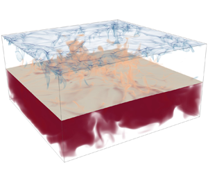
In this subsection, a qualitative description of the main features of the two-layer Rayleigh–Bénard convection is presented through a series of different flow visualizations. First, figure 3 presents snapshots of the temperature volumetric rendering, including the isosurface representing the location of the two-fluid interface. The activity of the thermal plumes is depicted clearly, especially at the top half of the cavity, where hotter plumes rise from the interface along with colder plumes descending from the top cooled wall. The plume activity typically feeds the large-scale circulation structures that sweep the boundary layers at their periphery. The bottom half of the cavity appears to be less active, with thicker thermal structures that occupy a significant portion of the available volume. As observed in single-phase thermal convection, the thermal structures become finer as the Rayleigh number increases, intensifying the thermal transport from the boundary layers to the large-scale circulation. On the contrary, based on the various snapshots in figure 3, the Weber number does not appear to have any obvious effect on the temperature field.

Figure 3. Snapshots of volume representations of the temperature field (semi-transparent coloured isosurfaces) and the interface (light brown surface at approximately mid-height) for the six different DNS cases. Red denotes a higher temperature compared to blue.
Focusing on the two-fluid interface as depicted in figure 3, its deformation is mostly visible for the  ${Ra}=10^6$ cases. For larger Rayleigh numbers, this deformation becomes less pronounced. More specifically, the r.m.s. values of the interface elevation $\eta _{rms}$ reduce by 69 % from ${Ra}=10^6$ to ${Ra}=10^8$ considering Weber number 100, and by 66 % considering Weber number 1000. The effects of the Weber number on the interface deformation are more clearly depicted in figure 4, where cases with larger Weber numbers exhibit a more noticeable deformation. As concerns the velocity fields, we note that the appearance of progressively smaller structures as the Rayleigh number increases well correlates with the ejected thermal plumes. This observation is more evident in the top half of the cavity, as the bottom half exhibits smaller temperature differences. The more qualitative observations discussed in this subsection will be verified in the quantitative statistical analysis presented in the following subsections.

Figure 4. Snapshots of  $x$–
$x$– $z$ planar representations of the temperature field, including streamlines (black lines with arrows) and the interface (white dashed line) for the six different DNS cases. Red denotes a higher temperature compared to blue.
3.2. Global properties
The analysis of global properties focuses on the interface temperature ( $\varTheta _\varGamma$) and the Nusselt and Reynolds numbers, which represent, in non-dimensional form, heat transfer and turbulence intensity, respectively. In this subsection, results extracted from the present DNS are compared against recently developed scaling laws with respect to the Rayleigh and Weber numbers. We note here that Liu et al. (Reference Liu, Chong, Yang, Verzicco and Lohse2022) have argued that the proposed scaling laws can hold for different Rayleigh numbers. Nonetheless, this hypothesis has not been assessed so far. The scaling laws for $\varTheta _\varGamma$, $Nu$ and $Re$ are based on the Grossmann–Lohse (GL) theory, which consists of two nonlinear equations, originating from the relations for the kinetic and thermal energy dissipation rates. For a multiphase problem, this set of equations is written for both layers separately (Liu et al. Reference Liu, Chong, Yang, Verzicco and Lohse2022):
 \begin{equation} ({Nu}_j-1)\,{Ra}_j\,{Pr}_j^{{-}2} = \dfrac{c_1\,Re_j^2}{g\left(\sqrt{\dfrac{Re_c}{Re_j}}\,\right)} + c_2\,Re_j^3, \end{equation}
 \begin{align} ({Nu}_j-1) &=
c_3\,Re_j^{1/2}\,Pr_j^{1/2}\sqrt{f\left[\dfrac{2c_0\,{Nu}_j}{\sqrt{Re_j}}\,g
\left(\sqrt{\dfrac{Re_c}{Re_j}}\,\right)\right]} \nonumber\\
&\quad
+c_4\,Pr_j\,Re_j\,f\left[\dfrac{2c_0\,{Nu}_j}{\sqrt{Re_j}}\,g\left(\sqrt{\dfrac{Re_c}{Re_j}}\,\right)\right],
\end{align}
\begin{align} ({Nu}_j-1) &=
c_3\,Re_j^{1/2}\,Pr_j^{1/2}\sqrt{f\left[\dfrac{2c_0\,{Nu}_j}{\sqrt{Re_j}}\,g
\left(\sqrt{\dfrac{Re_c}{Re_j}}\,\right)\right]} \nonumber\\
&\quad
+c_4\,Pr_j\,Re_j\,f\left[\dfrac{2c_0\,{Nu}_j}{\sqrt{Re_j}}\,g\left(\sqrt{\dfrac{Re_c}{Re_j}}\,\right)\right],
\end{align}
where indices  $j=1,2$ denote the corresponding parameters in the heavier and lighter fluids, respectively. The coefficients $c_{i}$, with $i=0,\ldots,4$, are the prefactors that are chosen as $c_{i}=0.922,8.05,1.38,0.487,0.0252$, as suggested in Stevens et al. (Reference Stevens, van der Poel, Grossmann and Lohse2013), together with $Re_c=(2c_0)^2$. The crossover functions $g$ and $f$ in (3.1) are given by $g(x)=(1+x^n)^{1/n}$ and $f(x)=x^n(1+x^n)^{1/n}$ with $n=4$ (Grossmann & Lohse Reference Grossmann and Lohse2000, Reference Grossmann and Lohse2001; Stevens et al. Reference Stevens, van der Poel, Grossmann and Lohse2013). The Prandtl number in (3.1) is computed as ${Pr}=\hat {\mu }_j\hat {c}_{p,j}/\hat {\zeta }_j$, while the Rayleigh numbers of each phase, ${Ra}_j$, read
 \begin{gather} {Ra}_1 = C_{tot}^3(1/2-\varTheta_\varGamma)\,{Ra}, \end{gather}
 \begin{gather}{Ra}_2=(1-C_{tot})^3(1/2+\varTheta_\varGamma)\,{Ra}\,\varLambda_\mu\varLambda_\zeta/ (\varLambda_\rho^2\varLambda_{c_p}\varLambda_\alpha), \end{gather}
where  $C_{tot}$ is the overall volume fraction of phase 1. Note that in Liu et al. (Reference Liu, Chong, Yang, Verzicco and Lohse2022), the properties ratios $\varLambda _\mu$, $\varLambda _\rho$, $\varLambda _{c_p}$ and $\varLambda _\alpha$ are omitted in (3.2) since they are considered equal to $1$, but are kept here for completeness. Therefore, the Nusselt numbers are defined as
 \begin{gather} {Nu}_1=\frac{\hat{Q}_1C_{tot}\hat{l}_z}{\hat{\zeta}_1(1/2-\varTheta_\varGamma)\,\Delta\hat{\varTheta}}, \end{gather}
 \begin{gather}{Nu}_2=\frac{\hat{Q}_2(1-C_{tot})\hat{l}_z}{\hat{\zeta}_2(1/2+\varTheta_\varGamma)\,\Delta\hat{\varTheta}}, \end{gather}
where the heat fluxes  $\hat {Q}_{1},\hat {Q}_{2}$ at the bottom and top walls are considered equal once a statistical equilibrium is reached, i.e. $\langle \hat {Q}_1\rangle _t=\langle \hat {Q}_2\rangle _t$. Equations (3.1) are applied to each layer separately, coupled to (3.2) and (3.3). The solution of this system of equations provides the values of $\varTheta _\varGamma$, ${Nu}_j$ and $Re_j$. Since the GL theory is implicit in ${Nu}_j$ and $Re_j$, an iterative procedure is required. Once ${Nu}_j$, $Re_j$ and $\varTheta _\varGamma$ are known, the global Nusselt number can be obtained readily from ${Nu}_j$ at one of the interface sides. Taking as reference the top wall and using the relation for $Nu_2$ in (3.3), the global $Nu$ reads
 \begin{equation} {Nu} = \dfrac{{\hat{Q}_2}\hat{l}_z}{\hat{\zeta}_2\,\Delta\hat{\varTheta}} = {Nu}_2\,\dfrac{1/2+\varTheta_\varGamma}{1-C_{tot}}. \end{equation}
 Similarly, we can define two global Reynolds numbers for the top ( $Re_{top}$) and bottom ( $Re_{bot}$) halves of the cavity. These quantities can be related to the turbulence in each phase, with $Re_{bot}=Re_1\,(\hat {\nu }_1/\hat {\nu }_{ref})/C_{tot}$ and $Re_{top}=Re_2c(\hat {\nu }_2/\hat {\nu }_{ref})/(1-C_{tot})$. Note that in the present set-up, $\hat {\nu }_{1}=\hat {\nu }_{2}=\hat {\nu }_{ref}$ and $C_{tot}=0.5$, therefore $Re_{bot}=2\,Re_{1}$ and $Re_{top}=2\,Re_{2}$.
The Nusselt and Reynolds numbers predictions are shown in figure 5, exhibiting excellent agreement against the corresponding scaling laws. This confirms the observation from Liu et al. (Reference Liu, Chong, Yang, Verzicco and Lohse2022) that the weak dependence on the Weber number is expected to hold as long as the interface does not break up and two separated layers can be clearly identified. Furthermore, the Reynolds number is approximately two times higher in the lighter fluid compared to the denser fluid, for all the Weber and Rayleigh numbers explored. This indicates significantly higher turbulence levels in the top half of the cavity.

Furthermore, as an alternative to (3.1), which requires an iterative solution, an approximation of  $\varTheta _\varGamma$ can be obtained explicitly. This approach has been proposed in Liu et al. (Reference Liu, Chong, Yang, Verzicco and Lohse2022) for multiphase thermal convection, and in Scapin et al. (Reference Scapin, Demou and Brandt2023) for evaporating Rayleigh–Bénard convection. The main idea is to employ a simplified scaling of the form ${Nu}_{j}=A_j\,{Ra}_j^{\gamma _j}\,{Pr}_j^{m_j}$ and to assume that the Rayleigh and Prandtl numbers of both phases are sufficiently similar to fall inside the same scaling regime of the GL theory, so that $A_1=A_2=A$, $\gamma _1=\gamma _2=\gamma$ and $m_1=m_2=m$. Then, by using (3.3) to express the ${Nu}_j$ and (3.2) to express the ${Ra}_j$, the following approximate relation for $\varTheta _\varGamma$ emerges:
 \begin{equation} \varTheta_\varGamma ={-}\frac{1}{2}+\left(1+\left(\frac{1-C_{tot}}{C_{tot}}\right)^{{(1-3\gamma)}/{(1+\gamma)}} \left(\frac{\varLambda_\rho^2\varLambda_{c_p}\varLambda_{\alpha}}{\varLambda_\mu}\right)^{{\gamma}/{(1+\gamma)}} \varLambda_\zeta^{{(1-\gamma)}/{(1+\gamma)}}\right)^{{-}1}. \end{equation}
Note that the Prandtl number dependence is typically omitted since the corresponding scaling exponent becomes  $0< m\ll 1$ for ${Pr}>0.5$ (Grossmann & Lohse Reference Grossmann and Lohse2000, Reference Grossmann and Lohse2001; Stevens et al. Reference Stevens, van der Poel, Grossmann and Lohse2013). In contrast to the implicit relations of the GL theory, (3.5) depends only on the various property ratios $\varLambda$ and the chosen scaling exponent $\gamma$. Figure 6 shows the interface temperature obtained from the DNS, compared against the predictions of the GL theory (3.1)–(3.3) and the predictions of the simplified scaling (3.5). The results of the simplified scaling assume the typical scaling exponent range $1/4\leq \gamma \leq 1/3$. As observed in figure 6, the DNS results from the low Weber number cases follow the GL theory closely. The higher Weber number cases deviate from the GL theory as the lower surface tension induces a stronger interface deformation, which influences the resulting scaling. Noteworthy is the fact that the simplified scaling provides a reliable estimation of $\varTheta _\varGamma$ for the different values of the Rayleigh number considered in the present study, with a maximum deviation of less than 2 % from the GL theory. Furthermore, despite its apparent simplicity, the simplified scaling directly highlights some important features of the equilibrium interface temperature $\varTheta _\varGamma$. First, we highlight that the weak dependence of $\varTheta _\varGamma$ on the Rayleigh number (absent in (3.5)) is confirmed by the DNS results, since the value of $\varTheta _\varGamma$ decreases by less than 3 % as $Ra$ increases from $10^6$ to $10^8$. Second, (3.5) enables us to quantify the role of each thermophysical property in modulating $\varTheta _\varGamma$, because each property ratio $\varLambda$ has its own scaling exponent. In particular, the density and thermal conductivity ratios have the largest exponents, representing the dominant sources of influence on the interface temperature $\varTheta _\varGamma$.

Figure 6. Average interface temperature  $\varTheta _\varGamma$ as a function of the Rayleigh number, for different Weber numbers. The GL theory predictions are calculated from (3.1)–(3.3), while the predictions of the simplified scaling are obtained from (3.5). The green region represents possible $\varTheta _\varGamma$ values for scalings $1/4<\gamma <1/3$, as per the simplified scaling.
We conclude this subsection by examining the thicknesses of the scaled thermal boundary layers at different locations in the cavity, which are shown in figure 7. The single-phase scaling of  ${Ra}^{-1/4}$ is used, as this scaling was proven to agree reasonably well with the interface temperature predictions in figure 6. Due to the presence of two fluid layers, the effective Rayleigh numbers ${Ra}_{1,2}$ defined in (3.2) are used to scale the thermal boundary layer thickness at the bottom and top halves of the cavity. The effective Rayleigh numbers consider the height and the temperature difference of the corresponding fluid layer, and for the parameters of the present study, can be simplified as ${Ra}_1 = {Ra}\,(0.5-\varTheta _\varGamma )/8$ at the bottom layer, and ${Ra}_2 = {Ra}\,(\varTheta _\varGamma +0.5)/8$ at the top layer. As shown in figure 7, this scaling is successful in collapsing the thicknesses of the thermal boundary layers that form on both the solid surfaces and the fluid interface. Note that this is true despite the variation of the Weber number, which, however, does not have a clear impact on the scaled thermal boundary layer thicknesses. As shown in figure 6, the Weber number has a minor influence on the interface temperature, which is not clearly noticeable when examining the thermal boundary layer thicknesses in figure 7. Indeed, the value of the interface temperature, $\varTheta _\varGamma$ appears in the definitions of both $h^{\theta }_{1,2}$ (2.10) and ${Ra}_{1,2}$ (3.2).

Figure 7. Scaled thermal boundary layer thickness at (a) the solid walls and (b) the interface. The scalings used are  ${Ra}_{1}^{-1/4}$ at the bottom and ${Ra}_{2}^{-1/4}$ at the top halves of the cavity, where ${Ra}_{1,2}$ are defined in (3.2).
3.3. Two-phase statistics
The vertical distributions of the average and r.m.s. phase indicator functions are shown in figures 8(a,b), respectively, with a focus on the region adjacent to the interface. As the Rayleigh number increases, the transition from one fluid to the other at  $z=0.5$ becomes sharper, as shown by the average distribution of the indicator function. This indicates the reduced interface deformation as the Rayleigh number increases. The same effect can be deduced from the r.m.s. values of the indicator function, where the fluctuations are shown to extend to a progressively smaller region as the Rayleigh number increases. This observation can be linked to the size of the thermal plumes that cause the interface deformation. In fact, with increasing Rayleigh number, the thermal plumes become progressively smaller (Zhou & Xia Reference Zhou and Xia2010), while the flow in the bulk becomes increasingly more homogeneous (Zhou, Sun & Xia Reference Zhou, Sun and Xia2008). Therefore, the stronger interface deformations at low Rayleigh numbers result from the larger thermal plumes in the cavity. Furthermore, increasing the Weber number leads to smoother profiles in the average distribution in figure 8(a), and larger fluctuating regions in figure 8(b). These trends are due to the decreased surface tension, leading to larger interface deformation. The interface deformation will be analysed further and characterized in § 3.4.

Figure 8. Vertical distributions of (a) average and (b) r.m.s. values of the indicator function for different values of the Rayleigh and Weber numbers.
The vertical profiles of the temperature field statistics are depicted in figure 9. The data in the figure suggest several considerations. First, the average temperature field in figure 9(a) reveals an increasingly sharper temperature profile as the Rayleigh number increases. Specifically, at the bottom and top walls of the cavity, the temperature gradients become larger (in absolute value) with increasing Rayleigh number, in accordance with the  ${Ra}^{-1/4}$ scaling of the thermal boundary layers in figure 7. The same characteristic is also observed in the temperature distribution next to the interface. In the bulk of the bottom half (approximately $z=0.2\unicode{x2013}0.4$) and the top half (approximately $z=0.6\unicode{x2013}0.8$), a nearly uniform temperature profile is observed, with a very weak dependence on the Rayleigh number. The temperature values in these regions are approximately 0.42 at the bottom half and $-0.05$ at the top half, approximately constant in all the cases. This significant asymmetry is mainly attributed to the different thermal conductivities on each side of the interface. Since the thermal conductivity of the denser fluid is an order of magnitude larger than that of the lighter fluid, the bulk temperature at the bottom half is much closer to the temperature at the bottom heated wall than that of the top half of the cavity. A final observation from figure 9(a) is that the average temperature distributions show negligible sensitivity to the Weber number.

Figure 9. Vertical distribution of (a) average and (b) r.m.s. values of the temperature field, for different values of the Rayleigh and Weber numbers. The line styles are the same as in figure 8.
The vertical distribution of the temperature r.m.s. fields is depicted in figure 9(b). The most distinct feature is the significantly smaller r.m.s. values at the bottom of the cavity compared to the top, hinting at a weaker turbulent state in the denser fluid, in line with the observations made from the instantaneous fields in § 3.1 and the Reynolds number predictions discussed in § 3.2. At the top of the cavity, two maxima are observed: a smaller one next to the top wall, and a larger one next to the two-phase interface, reinforced by the interface oscillation. For both peaks, the maximum values become smaller, and their location moves closer to the boundaries as the Rayleigh number increases. The same behaviour of the temperature r.m.s. field was observed in other single-phase studies, such as du Puits et al. (Reference du Puits, Resagk, Tilgner, Busse and Thess2007) for the turbulent convection in a cylindrical cell, and Demou & Grigoriadis (Reference Demou and Grigoriadis2019) in a cuboid cavity. Furthermore, increasing the Weber number leads to a noticeable increase in the temperature r.m.s. maximum values next to the interface. More specifically, the Weber number effects are stronger as the Rayleigh number increases. On the other hand, not surprisingly, the temperature r.m.s. values next to the top wall remain relatively unaffected with increasing Weber numbers.
Moving on to the statistics of the velocity field, we recall that since  $\langle u \rangle _{x,y,t} = \langle v \rangle _{x,y,t} = \langle w \rangle _{x,y,t} = 0$, the velocity r.m.s. reduces to $u_{rms}=\sqrt {\langle u^2 \rangle _{x,y,t}}$, $v_{rms}=\sqrt {\langle v^2 \rangle _{x,y,t}}$ and $w_{rms}=\sqrt {\langle w^2 \rangle _{x,y,t}}$, which corresponds to the square root of the single-phase kinetic energy per unit mass. Therefore, the velocity r.m.s. values are associated with the average kinetic energy per unit mass of the large-scale vortical structures in each fluid layer. Figures 10(a,b) show the vertical distributions of the vertical and horizontal components of the velocity r.m.s. field, respectively. As already mentioned, the turbulence at the bottom fluid layer is weaker compared to the top fluid layer, something that is clearly depicted in the r.m.s. profiles. Still, the rotation of the large-scale vortical structures is adequate in retaining relatively large velocity r.m.s. values in the denser fluid, in comparison to the temperature r.m.s. values in figure 9(b).

Figure 10. Vertical distribution of (a) the vertical and (b) the horizontal components of the velocity r.m.s. field, for different values of the Rayleigh and Weber numbers. The line styles are the same as in figure 8.
Focusing on the vertical velocity r.m.s. component, shown in figure 10(a), the different profiles exhibit a concave shape in each fluid layer, with a maximum at  $z=0.25$ and $z=0.75$, i.e. in the middle of the two layers. The curvature at the maxima decreases with increasing Rayleigh number, indicating a change in the circulation of the large-scale vortical structures. The actual maximum values behave non-monotonically, with larger maxima for the $Ra=10^7$ case. Moreover, the effects of the Weber number are more visible in the lighter fluid. They are much more pronounced for the lower Rayleigh number cases, as can be expected considering the stronger interface deformation in these cases. More specifically, the maximum vertical velocity r.m.s. component in the lighter fluid for $Ra=10^6$ increases noticeably with increasing Weber number, while there is no significant shift in the higher Rayleigh number cases. On the other hand, the horizontal velocity r.m.s. components, shown in figure 10(b), exhibit a similar shape to the temperature r.m.s. profiles in figure 9(b), with two maxima in each layer; one next to the solid wall, and one next to the two-fluid interface. The difference compared to the temperature profiles is that the maximum velocity r.m.s. values are approximately symmetric in each layer. As concerns variations of interface deformability, we observe trends similar to those observed for the vertical velocity r.m.s. distribution, with a more pronounced effect of the Weber number for smaller Rayleigh numbers.
3.4. Surface displacement
The dynamics of a mechanically perturbed interface is thoroughly discussed in the literature, usually referred to as wave-turbulence (Falcon & Mordant Reference Falcon and Mordant2022). By applying a statistically stationary large-scale perturbation (through either wind or mechanical excitation), the interface deforms into waves, whose elevation  $\eta (x,y,t)$ may vary significantly in time and space. Energy is redistributed towards small (dissipative) scales through nonlinear interactions, leading to a cascade process that is described thoroughly in the literature (Zakharov & Filonenko Reference Zakharov and Filonenko1967; Nazarenko Reference Nazarenko2011). Larger waves are generated through gravity forces, while smaller ones are governed by capillarity. The dispersion relation for the linear (small-amplitude) gravity-capillary waves reads (see Lamb Reference Lamb1993)
 \begin{equation} \hat{\omega}^2 = \left(\frac{\hat{\rho}_1-\hat{\rho}_2}{\hat{\rho}_1+\hat{\rho}_2}\,\hat{g} + \dfrac{\hat{\sigma}}{\hat{\rho}_1+\hat{\rho}_2}\,\hat{k}^2\right)\hat{k}, \end{equation}
where  $\hat {\omega }=2{\rm \pi} \hat {f}$ is the angular frequency (corresponding to time period $\hat {T}_f=1/\hat {f}$), and $\hat {k}=2{\rm \pi} /\hat {\lambda }$ is the wavenumber, corresponding to wavelength $\hat {\lambda }$. The first term on the right-hand side of (3.6) represents the contribution due to the gravity forces, while the second is the modulation due to capillary stresses. These two contributions are equal at the capillary wavenumber $\hat {k}_c=\sqrt {\hat {g}(\hat {\rho }_1-\hat {\rho }_2)/\hat {\sigma }}$, which, using (3.6), gives the capillary frequency $\hat {f}_c=\hat {g}^{3/4}(\hat {\rho }_1-\hat {\rho }_2)^{3/4}(\hat {\rho }_1+\hat {\rho }_2)^{-1/2}\hat {\sigma }^{-1/4}/(\sqrt {2}{\rm \pi} )$. The crossover scale is the capillary wavelength $\hat {\lambda }_c=2{\rm \pi} \sqrt {\hat {\sigma }/((\hat {\rho }_1-\hat {\rho }_2)\hat {g})}$: waves longer than this are driven by gravity, while smaller waves are driven by capillarity. For both the capillary ( $\hat {\lambda }>\hat {\lambda }_c$) and gravity ( $\hat {\lambda }<\hat {\lambda }_c$) regimes, theoretical predictions are available for spectra computed in both time, $\hat {S}_\omega =\langle |\tilde {\eta }(x,y,\omega )|^2 \rangle _{x,y}$ and space $\hat {S}_k=\langle |\tilde {\eta }(k_x,k_y,t)|^2 \rangle _{t}$, with $(\tilde {\cdot })$ being the Fourier transform. For gravity waves, Zakharov & Filonenko (Reference Zakharov and Filonenko1966) found that $\hat {S}_\omega \sim \hat {\omega }^{-4}$ and $\hat {S}_k\sim \hat {k}^{-5/2}$, while for capillary waves, the scaling laws $\hat {S}_\omega \sim \hat {\omega }^{-17/6}$ and $\hat {S}_k\sim \hat {k}^{-15/4}$ were obtained by Zakharov & Filonenko (Reference Zakharov and Filonenko1967).
The dispersion relation (3.6) is obtained by solving the linearized system composed of the Euler equations (in Fourier space) for an incompressible, irrotational and inviscid velocity field, and the equation for the interface elevation dynamics. However, the present system is quite different, with gravity effects not only producing waves at the interface (as in the aforementioned references) but also affecting the velocity field through buoyancy due to the dependency of density on the temperature. In fact, the full system of equations for the present configuration should comprise the Navier–Stokes equations, including not only viscosity but, more importantly, the effect of density variations that lead to the production of vorticity by the baroclinic torque, making (3.6) indicative only for the present study. Furthermore, the linearization employed to obtain (3.6) assumes that the nonlinearities of the problem provide only weak contributions. If nonlinearities become stronger, then the dispersion relation widens (Aubourg & Mordant Reference Aubourg and Mordant2016) and eventually deviates from the theoretical prediction in (3.6) (Herbert, Mordant & Falcon Reference Herbert, Mordant and Falcon2010).
Given this short overview, we move on to examine the results of the present simulations. Figure 11 shows the temporal spectrum  $\hat {S}_\omega$ of the wave elevation for each case, together with the scaling exponent predicted for gravity and capillary waves. When surface tension forces are higher, i.e. low $We$ (figures 11a–c), we observe that the capillary regimes ( $\hat {\omega }>\hat {\omega }_c$) can be observed over an extended range of frequencies, especially for the highest Rayleigh numbers under investigation here (see figures 11b,c). For the larger Weber number (figures 11d–f), we observe a region with a flatter spectrum around $\hat {\omega }\sim \hat {\omega }_c$, with a secondary peak and a scaling behaviour close to the capillary regime, $\hat {\omega }^{-17/6}$. The secondary peak becomes less pronounced with increasing Rayleigh number, while no capillary scaling can be observed at large wavenumbers. While it is difficult to explain the origin of the secondary peak, this is likely not connected to gravity waves. In fact, by increasing the Weber number, we do not find any consistent trend, with either the capillary or gravity power laws. This is indeed counter-intuitive, because increasing the Weber number should lead to the formation of larger waves, as the lower surface tension forces cannot withstand the local velocity fluctuations. Such waves should, in principle, behave as gravity waves, as $\hat {\omega } < \hat {\omega }_c$, but this is not observed in the spectra.

Figure 11. Temporal spectrum of the wave elevation  $\eta (x,y,t)$. In each plot, we show the spectrum $\hat {S}_\omega$ (black lines), the $-4$ power law for gravity waves (red dashed lines), and the $-17/6$ power law for capillary waves (blue dash-dotted lines), for (a–c) all cases at ${We}=100$, and (d–f) all cases at ${We}=1000$. The $x$-axes are normalized by the capillary frequency $\hat {\omega }_c=2{\rm \pi} \hat {f}_c$.
A similar behaviour is also observed consistently in the spatial spectrum, shown in figure 12. Again, at low  $We$ and high $Ra$ (figures 12b,c), the spatial spectra show a clean capillary wave range, which is observed only partially at low $Ra$ (figure 12a), and not observed at high $We$ ((figures 12d–f) except from the highest Rayleigh number. As shown in the temporal analysis, the spatial spectra also do not display a clean gravity waves range. In contrast, the secondary peak is clearly observed here for both Weber number values considered, although it is less visible at higher Rayleigh numbers. As evidenced, a pronounced secondary peak is associated with the disruption of the theoretical power-law behaviour of the gravity and capillary regimes.

Figure 12. Spatial spectrum of the wave elevation  $\hat {\eta }(x,y,t)$. In each plot, we show the spectrum $\hat {S}_k$ (black lines), the $-5/2$ power law for gravity waves (red dashed lines), and the $-15/4$ power law for capillary waves (blue dash-dotted lines), for (a–c) all cases at ${We}=100$, and (d–f) all cases at ${We}=1000$.
Next, we discuss the existence of the secondary peak. First, it is worth recalling that this is observed for frequencies (and wavenumbers) larger than the capillary scale. Similar deviations from the theoretical power laws are not unusual in wave turbulence (e.g. see Berhanu & Falcon Reference Berhanu and Falcon2013; Zonta, Soldati & Onorato Reference Zonta, Soldati and Onorato2015; Aubourg & Mordant Reference Aubourg and Mordant2016), and are typically attributed to dissipative effects or strong nonlinearities. In the present study, the most striking result is that the secondary peak in the spectrum attenuates at high Rayleigh number and low Weber number (a less pronounced peak appears in the spectrum), when a neater capillary wave regime can be observed. This observation can be linked to the interface fluctuations expressed through the r.m.s. values of the indicator function in figure 8(b), revealing smaller r.m.s. values at higher Rayleigh numbers. Considering as well the smaller values of the temperature r.m.s. distribution at higher Rayleigh numbers exhibited in figure 9(b) in combination with a less deformable interface at lower Weber numbers, the influence of nonlinear effects on the interface dynamics weakens.
To further investigate the interface dynamics, we display in figure 13 the space–time spectrum  $E_\eta (k,\omega )$ for all flows under investigation, and compare those with the dispersion relation for capillary and gravity-capillary waves. In all cases, we observe that neither the capillary nor the gravity-capillary dispersion relations provide good predictions for the maxima of the spectra, which could be expected in the current system. Nevertheless, most of the measured maxima lie between the two theoretical dispersion relations, revealing an intermediate regime created most likely by the combination of nonlinear effects due to buoyancy and viscous effects at small scales. For all the studied cases, we note a widening of the dispersion relation, meaning that nonlinearities are a critical aspect of these flows. Such widening may also affect some of the maxima, which therefore lie outside the theoretical dispersion relation for the capillary and gravity-capillary laws. Furthermore, there is a clear range of low frequencies where the footprints of the forcing can be observed (see Aubourg & Mordant Reference Aubourg and Mordant2016). On the other hand, it is important to notice that as $Ra$ increases, nonlinearities seem to decrease, and the maxima converge towards a line. This suggests that the energy transport mechanism at high Rayleigh and low Weber numbers is characterized by reduced nonlinearities, which may help to predict the effective interface area across which heat/mass is transferred.

Figure 13. Space–time spectrum  $\hat {E}_\eta (k,\omega )$ of the wave elevation $\hat {\eta }(x,y,t)$. In each plot, we show the spectrum contour, and the theoretical dispersion relation for capillary waves $\hat {\omega }_c^2 = [\hat {\sigma }/(\hat {g}(\hat {\rho }_1+\hat {\rho }_2))]\hat {k}^3$ is shown with a black dashed line, while the gravity-capillary dispersion relation from (3.6) is shown with a red dashed curve. Vertical and horizontal dotted black lines mark the capillary angular frequency and wavenumber. Black crosses indicate the maximum of $\hat {E}_\eta$ for each angular frequency. The configuration of the plots follows figures 11 and 12, i.e. (a–c) all cases at ${We}=100$, and (d–f) all cases at ${We}=1000$. Increasing Rayleigh numbers are shown from left to right: (a,d) ${Ra}=10^6$, (b,e) ${Ra}=10^7$, and (c,f) ${Ra}=10^8$.
4. Conclusions
This study provided a thorough analysis of how the Rayleigh and Weber numbers affect various quantities in two-layer Rayleigh–Bénard convection. For the adopted set of parameters, the Nusselt and Reynolds numbers, along with the interface temperature, were found to closely follow the Grossmann–Lohse scaling laws, with very little dependence on the Weber number. The same is true for the thermal boundary layers on both the solid boundaries and the two-fluid interface, which were found to scale with  ${Ra}^{-1/4}$ to a good approximation. Further investigation of the temperature field revealed two pronounced r.m.s. maxima in the top half of the cavity, the largest one located close to the two-fluid interface. As the Rayleigh number increases, the maxima move closer to the boundaries while their absolute values decrease. Moreover, increasing the Weber number increases the maximum values, more noticeably for the higher Rayleigh number cases. The r.m.s. fields of the horizontal velocity components exhibited similar profiles, albeit with approximately equal values in the two maxima locations. In contrast to the temperature fields, the Weber number effects on the velocity fields were found to be stronger for the lower Rayleigh number cases.
Significant effort was dedicated to presenting a comprehensive characterization of the two-fluid interface deformation. The simulation snapshots revealed stronger interface deformation for larger Weber numbers and smaller Rayleigh numbers, which was also confirmed by the mean and r.m.s. values of the indicator function. In addition, spectral analysis is used to characterize the interface dynamics. We observe that for large Rayleigh numbers and small Weber numbers, the interface deformation is smaller, and the scaling laws for capillary wave turbulence can be retrieved. At smaller Rayleigh numbers and larger Weber numbers, the large-scale circulation, in conjunction with the weaker surface forces, strongly deforms the interface. This is confirmed through the space–time spectrum, showing a non-negligible effect of large-scale forcing and nonlinearities that ultimately widen the dispersion relation. Nevertheless, the spectra become narrower when increasing the Rayleigh number, suggesting that in realistic applications at high Rayleigh numbers, the capillary scaling may help to predict the total interface through which heat and mass are exchanged.
An immediate extension of this work would be the consideration of realistic water–air parameters, including evaporation and non-Oberbeck–Boussinesq effects. The theoretical work by Scapin et al. (Reference Scapin, Demou and Brandt2023) suggested an analytical model for such flows, the predictions of which can be confirmed by three-dimensional DNS for different Rayleigh numbers. Such a study can provide invaluable insight into the heat transfer mechanism and interface dynamics, with relevant applications in atmospheric convection (Schumacher & Pauluis Reference Schumacher and Pauluis2010) and spent-fuel pools of nuclear power plants (Hay & Papalexandris Reference Hay and Papalexandris2020), among others.
Acknowledgements
A.D., N.S., M.C.-E. and L.B. acknowledge support from the Swedish Research Council (VR) via the multidisciplinary research environment INTERFACE, ‘Hybrid multiscale modelling of transport phenomena for energy efficient processes’ and grant no. 2016-06119. P.C. was supported by the University of Iceland Recruitment Fund grant no. 1515-151341, TURBBLY. The authors also acknowledge PRACE for awarding them access to MARCONI100 at CINECA, Italy, and SNIC for granting the use of Berzelius in grant no. Berzelius-2022-29. Additional CPU computing time for post-processing was provided by the Swedish National Infrastructure for Computing (SNIC) and by the Norwegian Research Infrastructure Services (NRIS, Pr. NN9561K). M.C-E. acknowledges the financial support given by the Department of Engineering ‘Enzo Ferrari’ of the University of Modena and Reggio Emilia through the action ‘FAR dipartimentale 2023/2024’, and the financial support by NextGenerationEU DD.3277, Ecosystem for Sustainable Transition of Emilia-Romagna (ECOSISTER) .
Declaration of interests
The authors report no conflict of interest.


