


1. Introduction
Theoretical and experimental analysis of Hele-Shaw flows has proved to be a particularly fruitful approach for investigating a wide variety of fundamental effects in fluid mechanics, such as viscous fingering (Paterson Reference Paterson1981; Islam & Gandhi Reference Islam and Gandhi2017), porosity (Homsy Reference Homsy1987; Huppert & Woods Reference Huppert and Woods1995) and bubble dynamics (Kopf-Sill & Homsy Reference Kopf-Sill and Homsy1988; Gaillard et al. Reference Gaillard, Keeler, Le Lay, Lemoult, Thompson, Hazel and Juel2021). Indeed, there has been extensive research into many aspects of Hele-Shaw flow (an extensive list of the research up to 1998 is given by Howison (Reference Howison1998), and a more up-to-date list is given in the review by Morrow et al. Reference Morrow, Moroney, Dallaston and McCue2021), including extensions to non-Newtonian and structured fluids, including polymers (Kawaguchi, Makino & Kato Reference Kawaguchi, Makino and Kato1997) and Oldroyd B fluids (Chaffin & Rees Reference Chaffin and Rees2018). However, perhaps surprisingly, there have only been limited studies of the Hele-Shaw flows of nematic liquid crystals (nematics) (Sengupta et al. Reference Sengupta, Tkalec, Ravnik, Yeomans, Bahr and Herminghaus2013a,Reference Sengupta, Pieper, Enderlein, Bahr and Herminghausb). Nematics possess internal structure due to their intrinsic orientational molecular order that can be described in terms of the average molecular orientation, which is expressed mathematically by a unit vector  $\boldsymbol {n}$ called the director (Stewart Reference Stewart2004). This structure gives rise to a host of interesting phenomena, including anisotropic viscous and elastic effects and, in the presence of an applied electric field, an induced polarisation in the nematic that can be utilised to orient the nematic director that then produces a change in the nematic effective viscosity (Stewart Reference Stewart2004). Although this effect has been extensively utilised in liquid crystal displays, it has yet to be employed in Hele-Shaw flow, in which context electrical control opens up new possibilities for flow manipulation.
Flow manipulation is key to many microfluidic-based technological and scientific applications involving microlevel mixing, sorting, cloaking and splitting of flows (Na et al. Reference Na, Yoon, Park, Lee and Lee2010; Urzhumov & Smith Reference Urzhumov and Smith2011; Taylor & Kaigala Reference Taylor and Kaigala2020; Loganathan et al. Reference Loganathan, Hsieh, Shi, Lu and Chen2023). Previously reported methods that can manipulate flows on demand (Paratore et al. Reference Paratore, Bacheva, Bercovici and Kaigala2022) have included single-phase methods which utilise micro/nanostructures (Wang et al. Reference Wang, Yang, Wu, Min, Chen and Hou2020) and porous media (Urzhumov & Smith Reference Urzhumov and Smith2011). The present work describes an alternative method using a localised and controllable viscosity change that enables user-controlled flow manipulation of an anisotropic liquid within a heterogeneous single-phase microfluidic device.
In this work, the flow of a nematic liquid crystal in a Hele-Shaw cell with an electrically controlled viscous obstruction is investigated using both a theoretical model based on the Ericksen–Leslie equations and physical experiments. The obstruction is created by temporarily electrically altering the viscosity of the nematic in a region of the cell across which an electric field is applied. After presenting the theoretical model, we validate the model experimentally for a circular cylindrical obstruction, demonstrating flow manipulation by varying the applied voltage.
2. Theoretical model
We begin by formulating a theoretical model using the equations describing the steady flow of a nematic liquid crystal in a Hele-Shaw cell with an electrically controlled viscous obstruction. In particular, we couple Gauss's Law for the electric potential with the standard Ericksen–Leslie theory for a nematic liquid crystal (Stewart Reference Stewart2004). The average molecular orientation of the nematic is described by the director,  $\boldsymbol {n} = \cos \theta \cos \phi \boldsymbol {\hat {x}} + \cos \theta \sin \phi \boldsymbol {\hat {y}} + \sin \theta \boldsymbol {\hat {z}}$, where $\boldsymbol {\hat {x}}$, $\boldsymbol {\hat {y}}$ and $\boldsymbol {\hat {z}}$ are the Cartesian coordinate unit vectors in the $x$-,
$x$-,  $y$- and $z$-directions, and $\phi (x,y,z)$ and $\theta (x,y,z)$ are the twist and tilt director angles (i.e. the angle the projection of $\boldsymbol {n}$ onto the $xy$-plane makes with the positive $x$-axis and the angle $\boldsymbol {n}$ makes with the positive $z$-axis), respectively. The electric field is written in terms of the electric potential $U(x,y,z)$, and the nematic flow is described by the fluid velocity $\boldsymbol {u} = u \boldsymbol {\hat {x}} + v \boldsymbol {\hat {y}} + w \boldsymbol {\hat {z}}$, where $u(x,y,z)$, $v(x,y,z)$ and $w(x,y,z)$ are the components of the velocity in the $x$-,
$x$-,  $y$- and $z$-directions, and the standard modified nematic pressure
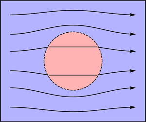
  $\tilde {p}(x,y,z)$. As shown in figure 1, we denote the ‘outside’ nematic region across which there is no applied electric field, in which variables have the subscript ${o}$, by $\varOmega _{o}$, and the ‘inside’ nematic region across which the electric field is applied, in which variables have the subscript ${i}$, by $\varOmega _{i}$. The boundary between $\varOmega _{i}$ and $\varOmega _{o}$ is denoted by $\partial \varOmega$.

Figure 1. A sketch of a perspective view of a Hele-Shaw cell containing an electrically controlled viscous obstruction. The nematic regions  $\varOmega _{i}$ (grey) and $\varOmega _{o}$ (light grey), and the boundary between them $\partial \varOmega$ (dark grey) are shown. The gap between the plates $D$, the length of the plates $L$, the width of the plates $W$, the origin (black dot), and the flow within the cell are also indicated.
We follow the approach of Cousins, Mottram & Wilson (Reference Cousins, Mottram and Wilson2024), who used a standard thin-film approach (Cousins et al. Reference Cousins, Bhadwal, Corson, Duffy, Sage, Brown, Mottram and Wilson2023) to study the flow of a nematic in a Hele-Shaw cell, but also accounting for the presence of the applied electric field. In particular, we non-dimensionalise Gauss's law and the Ericksen–Leslie equations so that  $x$ and $y$,
$y$,  $z$,
$z$,  $U$,
$U$,  $u$ and $v$,
$v$,  $w$, and $\tilde {p}$, are scaled with $L$,
$L$,  $\delta L$, $V$,
$V$,  $\mathcal {U}$, $\delta \mathcal {U}$, and $\eta _3\mathcal {U}/(\delta ^2L)$, respectively, where $\delta =D/L\ll 1$ is the small aspect ratio of the gap between the plates $D$ and the length of the plates $L$,
$L$,  $V$ is the voltage applied across the region $\varOmega _{i}$ in the $z$-direction, $\mathcal {U}=Q/(DW)$ is the characteristic flow speed for flow driven by a prescribed flux $Q$ and $W$ is the width of the plates, and $\eta _3$ is the isotropic viscosity of the nematic. Additionally, all viscosities are non-dimensionalised with $\eta _3$.
At leading-order in  $\delta \ll 1$, the thin-film Gauss's Law for the electric potential is given by
 \begin{equation} 0 = \left[(\epsilon_{{\perp}}+\Delta\epsilon\sin^2\theta){U}_z\right]_z, \end{equation}
where  $\epsilon _{\perp }$ is the constant dielectric permittivity perpendicular to the director, $\Delta \epsilon$ is the constant dielectric anisotropy, and the subscript $z$ denotes differentiation with respect to $z$. Equation (2.1) is subject to the boundary conditions that there is a unit potential difference between the electrodes that bound $\varOmega _{i}$ in the $z$-direction, namely $U=0$ on $z=0$ and $U=1$ on $z=1$ when $(x,y) \in \varOmega _{i}$, and there is a zero potential difference between the plates that bound $\varOmega _{o}$ in the $z$-direction, namely $U=0$ on $z=0$ and $z=1$ when $(x,y) \in \varOmega _{o}$. Integrating (2.1) twice with respect to $z$ and imposing the boundary conditions yields the electric potential $U$ in terms of the unknown tilt angle $\theta$.
The thin-film Ericksen–Leslie equations (Stewart Reference Stewart2004; Cousins et al. Reference Cousins, Mottram and Wilson2024) are given by the conservation of mass equation,
 \begin{equation} 0 = u_x+v_y+w_z, \end{equation}
the thin-film linear momentum equations,
 $$\begin{gather} \delta {{Re}} \, \dot{u} ={-}{\tilde{p}}_x + \left[g_1(\theta,\phi){u}_z + {g}_3(\theta,\phi){v}_z \right]_z, \end{gather}$$
 $$\begin{gather}\delta {{Re}} \, \dot{v} ={-}{\tilde{p}}_y + \left[{g}_3(\theta,\phi){u}_z + {g}_2(\theta,\phi){v}_z \right]_z, \end{gather}$$
 $$\begin{gather}\delta^3 {{Re}} \, \dot{w} ={-}{\tilde{p}}_{z}, \end{gather}$$
where  $\dot {u}$, $\dot {v}$ and $\dot {w}$ are the material time derivatives of $u$,
$u$,  $v$ and $w$, respectively, and the thin-film angular momentum equations,
 $$\begin{gather} 0 = \theta_{
zz}+\sin\theta\cos\theta\, \phi_z^2 - {Er}\, m(\theta)
\left(\cos\phi\, u_z+ \sin\phi\, v_z \right) - {Fz}
\sin\theta\cos\theta\ U_z^2,
\end{gather}$$
$$\begin{gather} 0 = \theta_{
zz}+\sin\theta\cos\theta\, \phi_z^2 - {Er}\, m(\theta)
\left(\cos\phi\, u_z+ \sin\phi\, v_z \right) - {Fz}
\sin\theta\cos\theta\ U_z^2,
\end{gather}$$ $$\begin{gather}0 = \left[ \cos^2 \theta\,
\phi_z \right]_z - \tfrac{1}{2}{Er}
(\gamma_1-\gamma_2)\sin\theta\cos\theta \left(\sin \phi\, u_z
-\cos \phi\, v_z \right).
\end{gather}$$
$$\begin{gather}0 = \left[ \cos^2 \theta\,
\phi_z \right]_z - \tfrac{1}{2}{Er}
(\gamma_1-\gamma_2)\sin\theta\cos\theta \left(\sin \phi\, u_z
-\cos \phi\, v_z \right).
\end{gather}$$
In (2.3)–(2.7),  $m(\theta )$, $g_1(\theta,\phi )$, ${g}_2(\theta,\phi )$ and ${g}_3(\theta,\phi )$ are the effective viscosity functions defined by
 $$\begin{gather} 2m(\theta) = \gamma_1 + \gamma_2 \cos2\theta, \end{gather}$$
 $$\begin{gather}g_1(\theta,\phi) = \eta_1\cos^2\theta\cos^2\phi+\eta_2\sin^2\theta+\cos^2\theta\sin^2\phi+\eta_{12}\sin^2\theta\cos^2\theta\cos^2\phi, \end{gather}$$
 $$\begin{gather}{g}_2(\theta,\phi) = \eta_1\cos^2\theta\sin^2\phi+\eta_2\sin^2\theta+\cos^2\theta\cos^2\phi+\eta_{12}\sin^2\theta\cos^2\theta\sin^2\phi, \end{gather}$$
 $$\begin{gather}{g}_3(\theta,\phi) = \eta_1\cos^2\theta\sin\phi\cos\phi-\cos^2\theta\sin\phi\cos\phi+\eta_{12}\sin^2\theta\cos^2\theta\sin\phi\cos\phi, \end{gather}$$
where  $\gamma _1$ and $\gamma _2$ are the non-dimensional rotational and torsional viscosities, and $\eta _1$, $\eta _2$, $\eta _3$ and $\eta _{12}$ are the non-dimensional Miesowicz viscosities (Miesowicz Reference Miesowicz1946). Also appearing in (2.3)–(2.7) are three non-dimensional groups, namely the Ericksen number ${Er} = \eta _3 D U/K = \eta _3 Q/(WK)$, the Reynolds number ${{Re}} = \rho D U/\eta _3 = \rho Q/(\eta _3 W)$, where $\rho$ is the constant density of the nematic, and the Freedericksz number ${Fz} = \epsilon _0 \Delta \epsilon V^2/K$, where $\epsilon_0$ is the permittivity of free space and $K$ is the Oseen–Frank one-constant elastic constant (Stewart Reference Stewart2004). The Freedericksz number is a ratio of the applied voltage and the Freedericksz voltage (Stewart Reference Stewart2004). Note that electric potential $U$ only enters the thin-film Ericksen–Leslie equations via the angular momentum equation (2.6). The thin-film Ericksen–Leslie equations (2.2)–(2.7) are subject to standard no-slip and no-penetration conditions on the plates, namely $u=v=w=0$ at $z=0$ and $z=1$.
We proceed by assuming that viscous effects and electromagnetic effects dominate elastic and inertial effects. In particular, we assume that  ${Er} \gg 1 \gg \delta {{Re}}$ in $\varOmega _{o}$ and that ${Er},{Fz} \gg 1 \gg \delta {{Re}}$ in $\varOmega _{i}$. As we shall see in § 4, this regime is representative of our experimental system for which ${Er} \approx 2\times 10^2$, $\delta {{Re}} \approx 10^{-6}$ and ${Fz} \approx 3\times (10\unicode{x2013}10^3)$. These assumptions have previously been found to be reasonable for nematic layers with similar dimensions and material parameters (Mottram et al. Reference Mottram, McKay, Brown, Russell, Sage and Tsakonas2016). In addition, note that the present model does not account for the presence of defects; however, while it is clear from the experimental results described in § 5 that defects occur, the good agreement between the experimental results and the predictions of the theoretical model suggests that they have little effect on the overall behaviour of the flow.
In  $\varOmega _{o}$, (2.3)–(2.7) are depth-averaged by integrating with respect to $z$ between $z=0$ and $z=1$ and rearranged to yield the well-known flow-alignment solution,
 $$\begin{gather} \hat{u}_{o} = \hat{u}_{o}(x,y) ={-}\dfrac{1}{12\eta_{o}} \frac{\partial \tilde{p}_{o}}{\partial x}, \quad \hat{v}_{o} = \hat{v}_{o}(x,y) ={-}\dfrac{1}{12\eta_{o}} \frac{\partial \tilde{p}_{o}}{\partial y}, \quad \hat{w}_{o} = 0, \end{gather}$$
 $$\begin{gather}\theta_{o} = \theta_{o}(z) = \begin{cases} +\theta_{L}, & \text{when} \ 0 \le z \le 1/2, \\ -\theta_{L}, & \text{when} \ 1/2 < z \le 1, \end{cases} \quad \tan \phi_{o}(x,y) = \dfrac{\hat{v}_{o}}{\hat{u}_{o}}, \end{gather}$$
where  $\eta _{o} = \eta _{L}$ is the local effective viscosity of a flow-aligned nematic, $\theta _{L}$ is the Leslie (or flow-alignment) angle given by the solution of $m(\theta )=0$ (Stewart Reference Stewart2004, § 5.2), and depth-averaged quantities are denoted by hats. The solution for $\theta _{o}$ in (2.13) is obtained from the leading-order-in- ${Er}$ angular momentum equation (2.6) together with the assumption that there is a narrow internal layer near $z=1/2$ across which $\theta _{o}$ changes from $\theta _{L}$ to $-\theta _{L}$, as is known to occur at sufficiently high flow rates (Stewart Reference Stewart2004, § 5.2) and has been described theoretically in the limit of small Leslie angle and large Ericksen number (Quintans Carou et al. Reference Quintans Carou, Duffy, Mottram and Wilson2006; Cousins et al. Reference Cousins, Wilson, Mottram, Wilkes and Weegels2020). The unknown pressure $\tilde {p}_{o}=\tilde {p}_{o}(x,y)$ is obtained from the depth-averaged conservation of mass equation (2.2),
 \begin{equation} \frac{\partial^2 \tilde{p}_{o}}{\partial x^2} + \frac{\partial^2 \tilde{p}_{o}}{\partial y^2} = 0. \end{equation}
 In  $\varOmega _{i}$, the thin-film Gauss's Law (2.1) and thin-film Ericksen–Leslie equations (2.2)–(2.7) are harder to solve. Specifically, the asymptotic regime ${Er},{Fz} \gg 1 \gg \delta {{Re}}$ leads to a system of partial differential equations that, in general, require a numerical approach. However, as we shall see shortly, the behaviour observed in the physical experiments can be captured by using an ansatz for the tilt angle $\theta _{i}$ of similar form to the solution for $\theta _{o}$ in (2.13). Equations (2.3)–(2.7) are depth-averaged and rearranged to yield
 $$\begin{gather} \hat{u}_{i} = \hat{u}_{i}(x,y) ={-}\dfrac{1}{12\bar{\eta}_{i}} \frac{\partial \tilde{p}_{i}}{\partial x}, \quad \hat{v}_{i} = \hat{v}_{i}(x,y) ={-}\dfrac{1}{12\bar{\eta}_{i}} \frac{\partial \tilde{p}_{i}}{\partial y}, \quad \hat{w}_{i} = 0, \end{gather}$$
 $$\begin{gather}\theta_{i} = \theta_{i}(z) = \begin{cases} +\bar{\theta}_{i}, & \text{when} \ 0 \le z \le 1/2, \\ -\bar{\theta}_{i}, & \text{when} \ 1/2 < z \le 1, \end{cases} \quad \tan \phi_{i}(x,y) = \dfrac{\hat{v}_{i}}{\hat{u}_{i}}, \end{gather}$$
where  $\bar {\theta }_{i}$ is an unknown constant tilt angle and
 \begin{equation} \bar{\eta}_{i}=\eta_1 \cos^2 \bar{\theta}_{i} + \eta_2 \sin^2 \bar{\theta}_{i} +\eta_{12}\sin^2\bar{\theta}_{i}\cos^2\bar{\theta}_{i} \end{equation}
is the local effective viscosity resulting from a balance of flow- and field-aligning torques in  $\varOmega _{i}$. This unknown constant tilt angle $\bar {\theta }_{i}$ and the unknown pressure $\tilde {p}_{i}=\tilde {p}_{i}(x,y)$ are then obtained from the depth-averaged thin-film angular momentum equation (2.6) and the depth-averaged conservation of mass equation (2.2), respectively, namely
 $$\begin{gather} \dfrac{{Er}\, m(\bar{\theta}_{i})}{4\bar{\eta}_{i}} \sqrt{\left(\frac{\partial \tilde{p}_{i}}{\partial x}\right)^2 + \left(\frac{\partial \tilde{p}_{i}}{\partial y}\right)^2} + {Fz} \sin \bar{\theta}_{i} \cos\bar{\theta}_{i} = 0, \end{gather}$$
 $$\begin{gather}\frac{\partial^2 \tilde{p}_{i}}{\partial x^2} + \frac{\partial^2 \tilde{p}_{i}}{\partial y^2} = 0. \end{gather}$$
Note that, from (2.13) and (2.16), the relevant twist angle,  $\phi _{o}$ or $\phi _{i}$, coincides with the direction of the depth-averaged flow in the $xy$-plane in both $\varOmega _{o}$ and $\varOmega _{i}$.
It is possible to reformulate the Laplace equations (2.14) and (2.19) in terms of complex potentials and to seek to determine semi-analytical solutions ( $\bar {\theta }_{i}$ must, in general, be obtained numerically) for a variety of shapes $\partial \varOmega$ using conformal mapping techniques; however, we do not pursue this approach here.
When  $\bar {\eta }_{i}>\eta _{o}$ the model describes the flow through and around a viscous obstruction. Far from $\partial \varOmega$ the flow is uniform and in the $x$-direction, while the pressure and the normal component of the fluid velocity are continuous across $\partial \varOmega$. Equations (2.14) and (2.19) subject to these boundary conditions are similar to the systems that describe many classical Hele-Shaw systems, including flow past a cylindrical obstruction (Hele-Shaw Reference Hele-Shaw1898) and flow through a cylindrical porous obstruction (Greenkorn et al. Reference Greenkorn, Haring, Jahns and Shallenberger1964).
In order to compare the predictions of the model with experimental observations, in the next section we consider the case of a circular cylindrical obstruction.
3. A circular cylindrical obstruction
We consider the case in which  $\varOmega _{i}$ is a circular cylinder with non-dimensional radius $R$ centred on the origin, such that $\varOmega _{o}$ is the region $x^2+y^2>R^2$, $\varOmega _{i}$ is the region $x^2+y^2< R^2$, and $\partial \varOmega$ is the circle $x^2+y^2=R^2$. Using an analogous method to that detailed in Greenkorn et al. (Reference Greenkorn, Haring, Jahns and Shallenberger1964) for a porous circular cylindrical obstruction, (2.14) and (2.19) subject to the appropriate boundary conditions can be solved analytically to yield
 \begin{equation} \tilde{p}_{o} ={-} 12 \left(1+\dfrac{\bar{\eta}_{i}-\eta_{o}}{\bar{\eta}_{i}+\eta_{o}}\dfrac{R^2}{x^2+y^2}\right) x \quad \text{and} \quad \tilde{p}_{i} ={-} \dfrac{24\eta_{o} \bar{\eta}_{i}}{\bar{\eta}_{i}+\eta_{o}} x, \end{equation}
and hence, from (2.18),  $\bar {\theta }_{i}$ satisfies the algebraic equation
 \begin{equation} \dfrac{12 {Er}\, \eta_{o} m(\bar{\theta}_{i})}{\eta_{o}+\bar{\eta}_{i}} = Fz \sin 2\bar{\theta}_{i}. \end{equation}
The range of accessible viscosities is set by the choice of nematic liquid crystal. The experiments were carried out using the well-characterised nematic material 4-Cyano-4-pentylbiphenyl, commonly referred to as ‘5CB’ (Dunmur, Fukuda & Luckhurst Reference Dunmur, Fukuda and Luckhurst2001). When  ${Fz} = 0$ (i.e. when $V = 0$), (3.2) yields $\bar {\theta }_{i} = \theta _{L} + k{\rm \pi}$, where $k$ is an integer, for which $\bar {\eta }_{i} = \eta _{o} = \eta _{L}$ ( $=0.73$ for 5CB), whereas in the limit ${Fz} \to \infty$ (i.e. when $\Delta \epsilon > 0$ and $V \to \infty$), (3.2) yields $\bar {\theta }_{i} \to (2k+1){\rm \pi} /2$, where again $k$ is an integer, for which $\bar {\eta }_{i} \to \eta _2$ ( $=3.23$ for 5CB), i.e. for 5CB, $\bar {\eta }_{i}$ can be more than four times larger than $\eta _{o}$.
With appropriate geometric and material parameters, (3.2) can be solved numerically for  $\bar {\theta }_{i}$ using a standard root-finding method, and the pressure is then given analytically by (3.1). The streamlines and the tilt angle of the director can then be determined from (2.12)–(2.13) and (2.15)–(2.16).
4. Experimental procedure
We now experimentally validate the theoretical model for a circular cylindrical viscous obstruction. In particular, a Hele-Shaw cell with gap  $D=(2.7\pm 0.4)\times 10^{-5}$ m, length $L=4.4\times \,10^{-2}$ m and width $W=2.0\times 10^{-2}$ m was filled with the nematic 5CB. The lower and upper plates of the device were made of coated borosilicate glass substrates, which were both coated with the amorphous fluorinated copolymer Teflon AF (Poly[4,5-difluoro-2,2-bis(trifluoromethyl)-1,3-dioxole-co-tetrafluoroethylene]), CAS 37626-13-4) to impart a homeotropic nematic surface alignment (Bhadwal et al. Reference Bhadwal, Mottram, Saxena, Sage and Brown2020). Transparent conducting indium tin oxide coatings on the upper and lower plates (ITO, $75$ nm thickness and $75\,\Omega /{\rm sq}$ resistivity) were patterned via direct write photolithography to provide an electrically addressable circular cylindrical region. The separation between the plates was maintained by using a PET (polyethylene terephthalate) spacer that also creates solid sidewalls in the Hele-Shaw cell at a dimensional position $y=\pm W/(2 L)$. The area over which the patterned electrodes overlapped defines the circular cylindrical nematic region (with a dimensional radius of $R=1.5\times 10^{-3}$ m) across which the electric field is applied, $\varOmega _{i}$, with an AC sinewave voltage ( $\,f = 10$ kHz, with r.m.s. voltage, $V$) between the electrodes in the $z$-direction, using a waveform generator connected to a voltage amplifier. A steady flow of 5CB within the cell was created by using two cylindrical glass capillaries (one the inlet, the other the outlet), which were connected to two holes in the upper plates using acrylic ferrules. The inlet was connected to a flow controller that established a constant volume flux of $Q=1\,\mathrm {\mu }{\rm Ls}^{-1}$. Finally, the entire cell was sealed with NOA-61 (Norland optical adhesive 61) and epoxy adhesive (Araldite Rapid) to prevent leaks. For each experiment, the voltage was applied for 30 s, and the flow profile data was captured during a 10 s time interval starting 5 s after the voltage was switched on. For 5CB, the Leslie angle is $\theta _{L} = 11.9^\circ$, and the viscosity $\bar {\eta }_{i}$ could be switched from a minimum of $\bar {\eta }_{i} = \eta _{o} \approx \eta _L = 0.0238$ Pa s at 0 V up to a maximum of $\bar {\eta }_{i} \approx \eta _2 = 0.1052$ Pa s at 50 V on a time scale ranging between 0.05 s at 50 V and 5 s at 5 V. When the voltage was removed, $\bar {\eta }_{i}$ relaxed back to $\eta _{o}$ on a time scale of approximately 1 s.
5. Results
Photographs of the Hele-Shaw cell viewed from above through crossed polarisers are shown in figure 2(a) for a range of voltages ( $V = 5$, $10$,
$10$,  $15$,
$15$,  $20$ and $50$ V). At the lowest voltage shown, $V=5$ V, very little difference in the flow in $\varOmega _{o}$ and $\varOmega _{i}$ is visible in the photographs; however, as the voltage increases from $V=10$ V to $V=20$ V, the colour of $\varOmega _{i}$ changes due to a reduction in the effective birefringence of the nematic layer resulting from the electrically controlled director reorientation out of the $xy$-plane (Dunmur et al. Reference Dunmur, Fukuda and Luckhurst2001). At the highest voltage shown, $V=50$ V, the strength of the electric field is sufficient to effectively align the director in the $z$-direction (i.e. the director aligns normal to the plates), resulting in $\varOmega _{i}$ becoming black as the effective birefringence of the nematic layer is reduced to zero. Note that the unidirectional flow in $\varOmega _{i}$ is a consequence of the circular shape of the obstruction. Other shapes would, in general, result in non-unidirectional flow in $\varOmega _{i}$. As figure 2 shows, increasing the viscosity in $\varOmega _{i}$ has the effect of deflecting the flow through and around the obstruction created in $\varOmega _{i}$. This deflection is shown in the time-averaged photographs of the cell shown in figure 2(b), which was generated using the minimum intensity projection method in ImageJ (Schneider, Rasband & Eliceiri Reference Schneider, Rasband and Eliceiri2012) for a sequence of $100$ frames extracted from experimental videos recorded at $10$ frames per second. In particular, figure 2(b) clearly shows that the degree of deflection increases as the voltage increases. Figure 2(b) also includes streamlines predicted by the theoretical model and shows them to be in excellent agreement with the experimental results.

Figure 2. (a) Photographs of the Hele-Shaw cell viewed from above through crossed polarisers (whose orientation is shown by the black arrows in (a) for  $V=5$ V), (b) time-averaged photographs of the cell with streamlines predicted by the theoretical model overlaid (shown by thin black lines) and (c) the local direction of the flow obtained from the image analysis (shown by red rods) and predicted by the theoretical model (shown by black rods) overlaid with a heat map of the angle between these directions, for $Q=1\,\mathrm {\mu }{\rm Ls}^{-1}$ and a range of voltages ( $V = 5$, $10$,
$10$,  $15$,
$15$,  $20$ and $50$ V). The white arrows in (a) show the flow speed and a white $0.5$ mm scale bar is shown in (a) for $V=5$ V. The colour of $\varOmega _{i}$ changes due to a reduction in the effective birefringence of the nematic layer.
In order to make a further comparison between the flow manipulation observed in the experiments and predicted by the theoretical model, we used the image analysis software package ImageJ (Schneider et al. Reference Schneider, Rasband and Eliceiri2012) with the plugin OrientationJ (Rezakhaniha et al. Reference Rezakhaniha, Agianniotis, Schrauwen, Griffa, Sage, Bouten, van de Vosse, Unser and Stergiopulos2012) to determine the local direction of the flow observed in the experiments. Figure 2(c) shows a comparison of the local direction of the flow obtained from the image analysis (shown by red rods) and predicted by the theoretical model (shown by black rods) overlaid with a heat map of the angle between these directions. Excellent agreement between the image analysis and the theoretical model is evident, especially at low voltages ( $V=5$ and $10$ V), where the results of the image analysis are often indistinguishable from the results predicted by the theoretical model. At high voltages ( $V=15$, $20$ and $50$ V), a similar agreement is achieved on the upstream (i.e. the left-hand) side of $\varOmega _{o}$; however, we note that the area over which the electrodes overlapped was not precisely circular, with a small polygonal shape on the downstream side (i.e. the right-hand) of $\varOmega _{i}$ (the shape of which is the black region shown in the photographs in figure 2(a) when $V=50$ V) which results in some disagreement between the image analysis and theoretical model on the downstream side of $\varOmega _{o}$. Additionally, at high voltages, the streaks in the experimental photographs (which are formed by moving defects elongated along the direction of the flow and hence visualise the streamlines) are reduced by the electric field as they pass through $\varOmega _{i}$, which leads to difficulty tracking the streamlines in the image analysis on the downstream side of $\varOmega _{o}$. In particular, figure 2 shows that the agreement between the image analysis and the theoretical model is good even in the vicinity of $\partial \varOmega$ at high voltages, where we might expect the thin-film model to break down.
Further confirmation of the very good agreement between the experimental results and the predictions of the theoretical model is provided in figure 3, which shows the local orientation of the flow (i.e. the angle the flow makes with the positive  $x$-axis) as a function of $y$ at various $x$-positions for the range of voltages. The error bars shown in figure 3 represent the standard deviation in the local orientation angle obtained by analysing three different images summed over three separate time intervals of duration 2.5, 5 and 10 s. Since the orientation of the flow is calculated using the streaks in the experimental photographs, which have different densities in different locations of the cell, an additional measure of confidence is given by the coherency of the local orientation of the flow (Rezakhaniha et al. Reference Rezakhaniha, Agianniotis, Schrauwen, Griffa, Sage, Bouten, van de Vosse, Unser and Stergiopulos2012). This coherency ranges from $0$ (ill-defined) to $1$ (perfectly defined) and is shown by the colour scale of each point in figure 3. Specifically, figure 3 shows that in $\varOmega _{i}$, for high voltages, where the streaks are of low density, there is a decrease in coherency.

Figure 3. The local orientation of the flow obtained from the image analysis (shown by the points) and predicted by the theoretical model (shown by the black lines) as functions of  $y$ at various $x$-positions (indicated by the blue arrow in the insets) relative to $\varOmega _{i}$, for $Q=1\,\mathrm {\mu }{\rm Ls}^{-1}$ and a range of voltages ( $V = 5$, $10$,
$10$,  $15$,
$15$,  $20$ and $50$ V). The coherency of the local orientation obtained from the image analysis is shown by the colour scale of each point.
6. Conclusions
In summary, the flow of a nematic liquid crystal in a Hele-Shaw cell with an electrically controlled viscous obstruction was investigated using both a theoretical model and physical experiments. The obstruction was created by temporarily electrically altering the viscosity of the nematic in a region of the Hele-Shaw cell across which an electric field was applied. The theoretical model was validated experimentally for a circular cylindrical obstruction, demonstrating user-controlled flow manipulation of an anisotropic liquid within a heterogeneous single-phase microfluidic device. This new approach can readily be extended to non-circular obstructions. Indeed, the use of self-registering shapes that inherently ensure precise alignment, or arrays of shapes for pixelated flow control, would be extremely interesting to investigate in future studies. Although the method demonstrated requires manufacturing patterned electrodes, this can be achieved using standard techniques such as photolithography, which, in the future, could be replaced entirely with modern thin-film transistor liquid crystal display architecture (Yamamoto Reference Yamamoto2012) and could pave the way for a complete pixel-level customisable flow manipulation in future single-phase Hele-Shaw cells.
Acknowledgements
The authors gratefully acknowledge Drs Brian R. Duffy (University of Strathclyde) and Ian C. Sage (Nottingham Trent University) for helpful discussions relating to the work.
Funding
This work was funded by the Engineering and Physical Sciences Research Council (EPSRC) via EPSRC research grants EP/T012986/1 and EP/T012501/2.
Declaration of interests
The authors report no conflict of interest.
Data availability statement
The data that support the findings of this study are openly available in Zenodo at https://doi.org/10.5281/zenodo.11173025.


 Open access