


1. Introduction
Flows past two-dimensional (2-D) bluff bodies, steady at low Reynolds number, generally become unstable to oscillatory perturbations, leading to vortex shedding. For example, the wake of a 2-D circular cylinder undergoes a Hopf bifurcation at the critical Reynolds number  $Re_c=47$, which breaks time invariance and results in the famous von Kármán vortex street. Other examples include flows past rectangular cylinders of various aspect ratios, including the square cylinder, but also ellipses, wedges, and so on. This first Hopf bifurcation seems to be generic to flows past isolated 2-D bluff bodies, although some 2-D flows first become unstable to stationary perturbations via a pitchfork bifurcation, like the planar sudden expansion (Fearn, Mullin & Cliffe Reference Fearn, Mullin and Cliffe1990) and the rotating circular cylinder (Pralits, Giannetti & Brandt Reference Pralits, Giannetti and Brandt2013).
Flows past three-dimensional (3-D) bluff bodies exhibit a richer series of bifurcations, whose sequence depends on the specific geometry. Often, wakes past axisymmetric bodies (e.g. thin disk, sphere, elongated bullet-shaped bodies) first become unstable to stationary perturbations of azimuthal wavenumber  $m=1$. The pitchfork bifurcation breaks the axisymmetry, leading to a steady wake deflected in some azimuthal direction, selected in practice by noise or imperfections. At larger Reynolds number, the flow undergoes a Hopf bifurcation, still with $m=1$, and the wake oscillates. For example, the stationary and oscillating critical Reynolds numbers are $Re_c^s \simeq 115$ and $Re_c^o \simeq 125$ for the wake of a thin disk, and $Re_c^s \simeq 210$ and $Re_c^o \simeq 275$ for the wake of a sphere (Natarajan & Acrivos Reference Natarajan and Acrivos1993; Fabre, Auguste & Magnaudet Reference Fabre, Auguste and Magnaudet2008; Gumowski et al. Reference Gumowski, Miedzik, Goujon-Durand, Jenffer and Wesfreid2008; Meliga, Chomaz & Sipp Reference Meliga, Chomaz and Sipp2009a). Axisymmetric rings also undergo an $m=1$ pitchfork bifurcation followed by an $m=1$ Hopf bifurcation for sufficiently small ratios of the torus diameter to the cross-section diameter (Sheard, Thompson & Hourigan Reference Sheard, Thompson and Hourigan2003). Interestingly, turbulent flows past axisymmetric bodies often exhibit multi-stability: the wake is almost always statically deflected in an arbitrary azimuthal direction, and randomly switches orientation with no preferred frequency. In other words, axisymmetry is broken instantaneously, but restored in the mean flow averaged over long times. This $m=1$ static symmetry breaking is reminiscent of the first laminar bifurcation, just as turbulent wakes past 2-D cylinders exhibit a large-scale coherent vortex shedding reminiscent of the first laminar bifurcation.
Rectangular prisms are some of the simplest non-axisymmetric 3-D bluff bodies. In a systematic numerical study, Marquet & Larsson (Reference Marquet and Larsson2015) investigated the linear stability of relatively thin rectangular plates (length-to-height ratio  $L/H=1/6$), and found that the nature of the first bifurcation depends on the frontal aspect ratio (width-to-height aspect ratio $W/H$). For large aspect ratios ( $W/H>2.5$), the wake becomes unstable via the Hopf bifurcation of an oscillatory eigenmode that breaks the planar symmetry across the smaller dimension while preserving the planar symmetry in the larger dimension. This is fully consistent with the limit of infinite aspect ratios, i.e. 2-D cylinders. For intermediate aspect ratios ( $2< W/H<2.5$), the wake still becomes unstable via a Hopf bifurcation but, remarkably, the oscillatory eigenmode breaks the planar symmetry across the larger dimension. For small aspect ratios ( $W/H<2$), the wake becomes unstable via a pitchfork bifurcation, which is reminiscent of the first bifurcation of the flow past a thin axisymmetric disk, and the stationary eigenmode breaks the planar symmetry across the smaller dimension.
A particular example of longer rectangular prisms is the cube ( $W=L=H$). Direct numerical simulations (DNS) by Saha (Reference Saha2004) and Meng et al. (Reference Meng, An, Cheng and Kimiaei2021) identified a pitchfork bifurcation at $Re_c \simeq 205\unicode{x2013}220$, leading to a steady wake with one planar symmetry. It is worth mentioning that since $W=H$, the two cross-flow directions (say, top/down and left/right) are equivalent, so there are actually two simultaneous bifurcations, each breaking one of the two planar symmetries. The flow then becomes unstable to oscillatory perturbations at $Re_c \simeq 250\unicode{x2013}270$, leading to oscillations that preserve one of the two planar symmetries. Those regimes have also been observed in the experiments of Klotz et al. (Reference Klotz, Goujon-Durand, Rokicki and Wesfreid2014).
Even longer rectangular prisms ( $L>W,H$) include Ahmed bodies and simplified ground vehicles, of strong interest in the automotive industry. Motivated by practical applications, many studies have been conducted at large $Re$ and in the presence of a horizontal ground (e.g. Grandemange, Gohlke & Cadot Reference Grandemange, Gohlke and Cadot2013; Cadot, Evrard & Pastur Reference Cadot, Evrard and Pastur2015; Brackston et al. Reference Brackston, García de la Cruz, Wynn, Rigas and Morrison2016; Evrard et al. Reference Evrard, Cadot, Herbert, Ricot, Vigneron and Délery2016; Barros et al. Reference Barros, Borée, Cadot, Spohn and Noack2017; Varon et al. Reference Varon, Eulalie, Edwige, Gilotte and Aider2017; Bonnavion & Cadot Reference Bonnavion and Cadot2018; Pavia, Passmore & Sardu Reference Pavia, Passmore and Sardu2018; Legeai & Cadot Reference Legeai and Cadot2020). Most of the time, the turbulent wake is not aligned with the body but rather deflected in one of two preferred states, and randomly switches between the two states, leading to a bimodal probability density function for the wake deflection. Interestingly, the direction of that deflection is dictated not by the ground but by the body geometry. For instance, bodies that are wider than tall have a wake deflected to the left or the right, i.e. in the direction parallel to the ground, and random switches restore the left/right planar symmetry in the long-term mean flow; conversely, bodies that are taller than wide have a wake deflected upwards or downwards, i.e. in the direction perpendicular to the ground (Grandemange et al. Reference Grandemange, Gohlke and Cadot2013). A recent turbulent study with no ground proximity (Legeai & Cadot Reference Legeai and Cadot2020) confirmed that the static deflection is in the larger direction. A similar scenario was observed in laminar experiments (Grandemange, Cadot & Gohlke Reference Grandemange, Cadot and Gohlke2012) and laminar simulations (Evstafyeva, Morgans & Dalla Longa Reference Evstafyeva, Morgans and Dalla Longa2017) for a wide Ahmed square-back body in ground proximity: the wake, initially symmetric, bifurcates to a steady deflected state at $Re_c \simeq 340$ and becomes oscillatory at $Re_c \simeq 410\unicode{x2013}430$, both bifurcations breaking the left/right planar symmetry.
To the best of our knowledge, there is no systematic study on rectangular prisms in the laminar regime, and several questions remain unanswered. For instance, what are the critical Reynolds numbers and the properties of the first linear instabilities? Are those instabilities oscillatory or stationary? Which spatial symmetry do they break? Is one of these laminar instabilities persisting at larger Reynolds number in the form of the symmetry breaking observed in the turbulent regime? What kind of flow is expected in the nonlinear regime? In the present study, we address those questions by investigating the stability of rectangular prisms of fixed width-to-height aspect ratio  $W/H=1.2$, and varying length-to-height ratio $L/H$. We also vary the front fillet radius $R$ to assess the effect of rounding the leading edges, which is known to modify instability thresholds in 2-D rectangular cylinders (see e.g. Park & Yang Reference Park and Yang2016; Chiarini, Quadrio & Auteri Reference Chiarini, Quadrio and Auteri2021); this allows us to consider geometries ranging from thin plates with sharp edges (as in Marquet & Larsson Reference Marquet and Larsson2015) to Ahmed bodies with rounded leading edges.
After describing the flow configuration in § 2 and the numerical methods in § 3, we characterise the steady symmetric base flow in § 4. We then perform a 3-D linear stability analysis in § 5. Anticipating the results, we find that the flow always become unstable via two pitchfork bifurcations, at two critical Reynolds numbers close to one another. In almost all cases, the first mode breaks the top/down symmetry (across the smaller dimension), and the second mode breaks the left/right symmetry (across the longer dimension). In § 6, we then study the nonlinear regime with a weakly nonlinear (WNL) analysis incorporating the two stationary modes for a reference Ahmed body. We show that as  $Re$ increases, a top/down symmetry-breaking state appears first, but is eventually replaced by a left/right symmetry-breaking state. A series of fully nonlinear DNS confirms the results. Finally, we observe that the WNL bifurcation sequence is robust to geometric variations for values of $W$ and $L$ typical of common Ahmed bodies.
2. Flow configuration
We consider the incompressible flow of a Newtonian fluid past a 3-D rectangular prism. The planar faces of the bluff body define a Cartesian coordinate system. The incoming flow is  $\boldsymbol {U}_\infty = (U_\infty,0,0)^{\rm T}$, i.e. the body's roll, pitch and yaw are zero. For convenience, we call the $x$,
$x$,  $y$ and $z$ directions the streamwise, lateral and vertical directions, respectively. We can therefore say that the front/rear faces of the body are normal to the $x$ direction, left/right faces to the $y$ direction, and upper/lower faces to the $z$ direction. Similarly, we define the body dimensions as length $L$, width $W$ and height $H$ (cf. figure 1). Bodies with rounded front edges are also considered, with a fillet radius $R$. Hereafter, all quantities are made dimensionless using the body height $H$ as reference length and free-stream velocity $U_\infty$ as reference velocity.

Figure 1. Sketch of the flow configuration. A rectangular prism of height  $H$, width $W$, length $L$ and front edge fillet radius $R$ is aligned with the incoming flow $\boldsymbol {U}_\infty = (U_\infty,0,0)^{\rm T}$. (a) Top, side and front views. (b) A 3-D view, highlighting the symmetry planes $y=0$ and $z=0$, and the quarter-body (darker) used in our linear and WNL calculations. In this sketch, the specific geometry $W/H=1.2$, $L/H=3$, $R/H=0.3472$ is shown, a reference Ahmed body that we also investigate with DNS around the full body.
In this study, we fix the body width  $W=1.2$, except in the final part of the WNL analysis (§ 6.4). The length is varied between $L=1/6 \simeq 0.167$ (thin plate orthogonal to the flow) and $L=3.8$ (similar to some Ahmed bodies). The fillet radius of the front edges is varied between $R=0$ (sharp edges) and $R = \min (0.5, L)$ (fully rounded edges, with either upper/lower fillets meeting tangentially and the front face vanishing, or all fillets reaching the rear face and all lateral faces vanishing). In between, the value $R= 100/288 \simeq 0.347$ is typical of Ahmed bodies. See figure 2 for an overview.

Figure 2. Rectangular prisms of different lengths  $L$ and front fillet radii $R$.
$R$.
The velocity field  $\boldsymbol {u}(\boldsymbol {x},t)=(u,v,w)^{\rm T}$ and pressure field $p(\boldsymbol {x},t)$ are solutions of the incompressible Navier–Stokes (NS) equations, expressing the conservation of mass and momentum, and written in the dimensionless form
 \begin{equation} \boldsymbol{\nabla} \boldsymbol{\cdot} \boldsymbol u = 0,\quad \partial_t \boldsymbol{u} + (\boldsymbol{u} \boldsymbol{\cdot} \boldsymbol{\nabla}) \boldsymbol{u} ={-}\boldsymbol{\nabla} p + \frac{1}{Re}\,\nabla^2 \boldsymbol{u},\end{equation}
where the Reynolds number  $Re=U_\infty H/\nu$ is based on the free-stream velocity, the body height and the fluid kinematic viscosity. Throughout this paper, all lengths and velocities are made dimensionless using $H$ and $U_\infty$, respectively.
3. Numerical methods
In this study, two different numerical methods are used. The nonlinear base flow calculation, linear stability analysis and WNL stability analysis are performed with the finite element software FreeFEM (Hecht Reference Hecht2012), while DNS are performed with the finite volume software OpenFOAM (Greenshields Reference Greenshields2022).
For finite element calculations, we first build a tetrahedral mesh using the 3-D finite element mesh generator Gmsh (Geuzaine & Remacle Reference Geuzaine and Remacle2009), with mesh nodes strongly clustered near the body surface. We choose the domain  $\varOmega ' = \{ x,y,z \, | \, {-10} \leq x \leq 20;\ 0 \leq y,z \leq 10 \}$ (approximately similar to that in Evstafyeva et al. Reference Evstafyeva, Morgans and Dalla Longa2017) and the mesh density so as to achieve a tradeoff between accuracy and computational effort. See Appendix A for more details about the mesh characteristics and convergence studies on mesh density and domain size. We use the same mesh to solve the base flow problem (4.1a,b), the direct and adjoint eigenvalue problems (5.6) and (5.11), and the linear problems (6.13)–(6.16) appearing in the WNL analysis and the coefficients (6.22)–(6.27) of the amplitude equations (6.20)–(6.21). We discretise the weak form of the equations to be solved with FreeFEM, using a basis of Arnold–Brezzi–Fortin MINI-elements, i.e. P1 (linear) elements for pressure, and P1b (linear enriched with a cubic bubble function) elements for each velocity component. We solve for the nonlinear base flow using an iterative Newton method. Linear systems involved in each Newton iteration and in the WNL analysis are inverted with the PETSc library. Eigenvalue problems are solved with the SLEPc library, using a Krylov–Schur method to obtain a set of eigenvalues closest to a given complex shift, together with the associated eigenmodes. Calculations are repeated with a series of shifts chosen so as to obtain all leading eigenvalues in a range of frequencies of interest (typically $|\omega | \leq 1$). All problems involve several millions of degrees of freedom, and are solved in parallel using a domain-decomposition method on 24–48 processes. Typical calculation times are of the order of one hour for the base flow at a few $Re$ values, and one hour for a few eigenvalues.
The DNS are carried out on the same domain as the linear and WNL analyses, without assuming a priori symmetry conditions, i.e. on the full domain  $\varOmega = \{ x,y,z \, | \, {-10} \leq x \leq 20,\ {-10} \leq y,\ z \leq 10 \}$. The mesh is generated exploiting the routine snappyHexMesh. As starting point, an initial Cartesian mesh generated with blockMesh is employed, with 5 cells per unit length. Four nested regions of increasing refinements are introduced around the solid body, to guarantee $0.5\times 10^6$ cells per unit volume in the vicinity of the body. To test convergence, the same mesh generation strategy is used, employing 2.5 and 10 cells per unit length as initial mesh; the drag coefficient is used as a convergence criterion, showing differences of less than 1.3 % between the two finest meshes. A time-marching strategy is employed to calculate the steady flow solution, based on a Crank–Nicolson scheme with initial uniform solution equal to $\boldsymbol {U}=(U_{\infty },0,0)^{\rm T}$. The NS equations are solved by exploiting the PIMPLE method, which decouples velocity from pressure. The spatial discretisation of each equation is based on the finite volume method with Gauss linear integration scheme, assuring second-order precision in both time and space. Typical calculation times are of the order of one week for one nonlinear flow simulated over $10^3$ convective times.
4. Base flow
In this section, we characterise the steady base flow  $\boldsymbol q_0(\boldsymbol x) = (\boldsymbol u_0 ,p_0)^{\rm T}$ past rectangular prisms of various lengths $L$ and fillet radii $R$, for a fixed width $W = 1.2$. The base flow is a solution of the steady NS equations
 \begin{equation} \boldsymbol{\nabla} \boldsymbol{\cdot} \boldsymbol u_0 = 0,\quad (\boldsymbol{u}_0 \boldsymbol{\cdot} \boldsymbol{\nabla}) \boldsymbol{u}_0 ={-}\boldsymbol{\nabla} p_0 + \frac{1}{Re}\,\nabla^2 \boldsymbol{u}_0 \end{equation}
in the fluid domain  $\varOmega$. We look for base flows that have the same symmetries as the body: reflectional symmetries in the $y$ and $z$ directions (i.e. symmetry with respect to the vertical $x$–
$x$– $z$ plane and the horizontal $x$–
$x$– $y$ plane, respectively). We take advantage of these symmetries to reduce the computational cost. Namely, we solve the stationary NS equations (4.1a,b) on the quarter-space $\varOmega ' = \{ x,y,z \, | \, y\geq 0,\ z\geq 0 \}$ instead of the full space $\varOmega$, and we impose the following symmetry conditions on the symmetry planes:
 \begin{equation} \left.\begin{gathered} \partial_y u_0 = v_0 = \partial_y w_0 = 0 \quad \mbox{on the } y=0 \mbox{ plane}, \\ \partial_z u_0 = \partial_z v_0 = w_0 = 0 \quad \mbox{on the } z=0 \mbox{ plane}. \end{gathered}\right\} \end{equation}
Additionally, we impose a free-stream velocity  $\boldsymbol {u}_0 = (1,0,0)^\textrm {T}$ on the inlet plane, a no-slip condition $\boldsymbol u_0 = \boldsymbol 0$ on the body surface, a stress-free condition $-p_0 \boldsymbol n + Re^{-1}\,\boldsymbol {\nabla } \boldsymbol u_0 \boldsymbol {\cdot } \boldsymbol n = \boldsymbol 0$ on the outlet plane (with $\boldsymbol n$ the outward unit normal vector), and symmetry conditions identical to (4.2) on the remaining (lateral and upper) boundaries.
4.1. Effect of  $Re$
$Re$

We start by illustrating the effect of the Reynolds number for a selected geometry, namely  $L=3$ and $R=0$. Figures 3 and 4 show cuts of the streamwise velocity field and contours of zero streamwise velocity for different values of $Re$. There are several recirculation regions found around the prism: a ‘wake recirculation’ originating from the trailing edges, and ‘side recirculations’ originating from the leading edges. Figure 5(a) shows the variation in length of these regions: the wake recirculation length $l_w$, measured along the symmetry axis $y=z=0$, and the side recirculation lengths $l_s$, measured in the symmetry planes on the left/right faces ( $|y|=W/2$, $z=0$) and on the upper/lower faces ( $y=0$, $|z|=H/2$). Since $W>H$, side recirculations on the upper/lower faces are slightly longer than those on the left/right faces. Their length is seen to increase monotonically with $Re$ in the investigated range of Reynolds number, until they extend all the way down to the trailing edges ( $l_s = L = 3$) and connect with the wake recirculation at $Re \simeq 500$. By contrast, the length of the wake recirculation varies non-monotonically, reaching a maximum at $Re \simeq 350$. The maximum backflow, i.e. the minimum streamwise velocity along the symmetry axis, $U_b = \min u_0(x,0,0)$, decreases in the investigated range of $Re$ from $-$0.18 to $-$0.26 (inset of figure 5a). Its non-monotonic variation seems correlated with that of $l_w$. In addition, figure 4(a) shows that although the width of the backflow region in the wake increases monotonically, its height varies non-monotonically. As a result, vertical cross-sections of the backflow region change from circles to wider-than-tall ellipses. It is important to note that 2-D cuts in the symmetry planes $y=0$ and $z=0$ provide only partial information about the 3-D structure of the flow. The 3-D views in figures 4(b,c) show, for instance, that reattachment occurs farther downstream in the symmetry planes than away from them, and that the backflow regions on the sides of the prism become non-convex for large enough $Re$. All this suggests that even before they merge at $Re \simeq 500$, the recirculation regions on the sides and in the wake undergo some 3-D reorganisation, which affects $l_w$ and $U_b$.

Figure 3. Streamwise velocity  $u_0$ of the base flow past a rectangular prism, $W=1.2$, $L=3$, $R=0$, in the planes $z=0$ (top view), $y=0$ (side view) and $x=2.5$ (rear view), for (a) $Re=150$, (b) $Re=250$, (c) $Re=350$, and (d) $Re=450$.

Figure 4. Contours of zero streamwise velocity  $u_0=0$ for the base flow past a rectangular prism, $W=1.2$, $L=3$, $R=0$: (a) in the planes $z=0$ (top view $a1$), $y=0$ (side view $a2$) and $x=2.5$ (rear view $a3$), for $Re=150$, 250, 350 and 450; and 3-D views for (b) $Re=250$ and (c) $Re=450$. While the width of the wake recirculation increases monotonically with $Re$ (plot $a1$), its length and height vary non-monotonically (plot $a2$).

Figure 5. Base flow past a rectangular prism,  $W=1.2$, $L=3$, $R=0$. (a) Length of the wake recirculation and side recirculations. Dashed line is $l_s=L=3$, when the side recirculations reach the end of the body and connect with the wake recirculation. Inset: maximum backflow $U_b$. (b) Drag coefficient.
At larger  $Re$, the wake recirculation becomes substantially longer, wider and taller (not shown) as it merges with the side recirculations, and the backflow becomes stronger. We do not, however, focus on this topological change of the base flow because bifurcations of interest occur at smaller $Re$, as will become clear in §§ 5 and 6.
Figure 5(b) shows the evolution of the drag coefficient,
 \begin{equation} C_x = \frac{F_x}{\tfrac{1}{2} \rho U_\infty^2 W H},\quad \mbox{where } F_x ={-} \oint_{\varGamma_{b}} \left( \boldsymbol{\sigma}_0 \boldsymbol{\cdot} \boldsymbol{n} \right) \boldsymbol{\cdot} \boldsymbol{e}_x \,\mathrm{d}\varGamma, \end{equation}
where  $\varGamma _b$ is the surface of the full body, and the stress tensor $\boldsymbol {\sigma }_0 = -p_0 \boldsymbol {I} + Re^{-1}\,\boldsymbol {\nabla } \boldsymbol u_0$ includes pressure and viscous effects. The drag coefficient decreases with $Re$, as do both pressure and viscous contributions, which is typically of bluff bodies in the laminar regime (see e.g. Henderson (Reference Henderson1995) for the 2-D circular cylinder wake). As $Re$ increases, the viscous contribution becomes much smaller than its pressure counterpart, because the side recirculations extend over a larger body surface area while the wake recirculation is not modified substantially.
4.2. Effect of $L$

We now investigate the effect of the length  $L$ on the steady base flow past bodies with sharp edges ( $R=0$). For the sake of illustration, we choose $Re=250$ (which will prove to be close to the critical Reynolds number in § 5). Figure 6 shows the streamwise velocity field for $L$ between $1/6$ and 3. For large $L$, the flow separates at the leading edges and reattaches onto the body, as described previously; the flow then re-separates at the trailing edges with a small angle with respect to the streamwise direction, which leads to a rather narrow and short wake recirculation. As $L$ decreases, the side recirculations and the wake merge, and the wake recirculation becomes longer and the backflow stronger. The overall flow also becomes increasingly different in the two symmetry planes $y=0$ and $z=0$: separation occurs with a larger angle from the upper/lower leading edges, and the wake becomes significantly taller, but not wider.

Figure 6. Streamwise velocity  $u_0$ of the base flow past rectangular prisms, $W=1.2$, $R=0$, at $Re=250$, in the planes $z=0$ (top view), $y=0$ (side view) and $x=2.5$ (rear view), for (a) $L=1/6$, (b) $L=0.5$, (c) $L=1$, (d) $L=1.5$, (e) $L=2$, and (f) $L=2.5$.
These qualitative observations are confirmed in figure 7(a): the length of the wake recirculation decreases with  $L$, while the side recirculations (disconnected from the wake only when $L > l_w$) keep a fairly constant length. The backflow $U_b$ (inset) is much stronger when $L\lesssim 1.5$, i.e. when the side and wake recirculations are connected.

Figure 7. Base flow past rectangular prisms,  $W=1.2$, $R=0$, at $Re=250$. (a) Length of the wake recirculation and side recirculations. Dashed line is $l_s=L$, when the side recirculations reach the end of the body and connect with the wake recirculation. Inset: maximum backflow $U_b$. (b) Drag coefficient.
Figure 7(b) shows that the drag coefficient varies non-monotonically with  $L$, reaching a minimum for $L \simeq 1.5$. This is the result of a competition between pressure and viscous effects. Pressure drag decreases with $L$, as longer bodies have narrower wakes, associated with a weaker front/rear pressure difference. Conversely, viscous drag increases with $L$, as longer bodies are subjected to positive wall shear stress over a wider surface area.
4.3. Effect of $R$

We now investigate the effect of the fillet radius  $R$ on the steady base flow past bodies of lengths $L=1$ and $L=3$. Figure 8 shows the streamwise velocity field for $L=3$ and several fillet radius values. Rounding the front edges clearly suppresses the side recirculations. It turns out that a very small fillet, $R \gtrsim 0.05$, is sufficient to keep the flow attached to the body. For the shorter body, $L=1$, this also makes the wake recirculation narrower and slightly shorter. For the longer body, $L=3$, this has no visible effect on the wake recirculation. Figure 9 confirms that the wake recirculation length is slightly reduced for $L=1$ and barely affected for $L=3$. The backflow (inset) follows different trends for $L=1$ and $L=3$.

Figure 8. Streamwise velocity  $u_0$ of the base flow past rectangular prisms, $W=1.2$, $L=3$, at $Re=250$, in the planes $z=0$ (top view), $y=0$ (side view) and $x=2.5$ (rear view), for (a) $R=0$, (b) $R=0.05$, (c) $R=0.1$, (d) $R=0.2$, (e) $R=0.3472$, and (f) $R=0.5$.

Figure 9. Length of the wake recirculation in the flow past rectangular prisms,  $W=1.2$, at $Re=250$, for (a) $L=1$, and (b) $L=3$. Insets: maximum backflow.
Finally, figure 10 shows that  $R$ has a strong effect on drag. For both $L=1$ and $L=3$, pressure drag decreases with $R$, as a result of the reduced front area. By contrast, viscous drag increases because boundary layers stay attached to the body. Overall, pressure effects are stronger and $C_x$ decreases.

Figure 10. Drag coefficient of rectangular prisms,  $W=1.2$, at $Re=250$, for (a) $L=1$, and (b) $L=3$.
5. Linear stability analysis
We now investigate the linear stability of the steady base flows  $\boldsymbol q_0(t)$ computed in § 4. We therefore consider small-amplitude perturbations
 \begin{equation} \boldsymbol q(\boldsymbol x,t) = \boldsymbol q_0(\boldsymbol x) + \epsilon\,\boldsymbol q_1(\boldsymbol x,t), \end{equation}
where  $0 < \epsilon \ll 1$. Injecting (5.1) in the NS equations (2.1a,b) yields at order $\epsilon$ the linear dynamics of the perturbations $\boldsymbol q_1 (\boldsymbol x,t) = (\boldsymbol u_1, p_1)^\textrm {T}$:
 \begin{equation} \boldsymbol{\nabla} \boldsymbol{\cdot} \boldsymbol u_1 = 0,\quad \partial_t \boldsymbol u_1 + (\boldsymbol{u}_0 \boldsymbol{\cdot} \boldsymbol{\nabla}) \boldsymbol{u}_1 + (\boldsymbol{u}_1 \boldsymbol{\cdot} \boldsymbol{\nabla}) \boldsymbol{u}_0 ={-}\boldsymbol{\nabla} p_1 + \frac{1}{Re}\,\nabla^2 \boldsymbol{u}_1. \end{equation}
We rewrite (5.2) in the compact form
 \begin{equation} \mathcal{B}\,\partial_t {\boldsymbol q}_1 + \mathcal{A} {\boldsymbol q}_1 = \boldsymbol{0}, \end{equation}
with the linear operators
 \begin{equation} \mathcal{A} = \left(\begin{array}{cc} \mathcal{C}(\boldsymbol{u}_0, \cdot) - Re^{{-}1}\,\nabla^2 ({\cdot}) & \boldsymbol{\nabla} (\cdot) \\ \boldsymbol{\nabla}\boldsymbol{\cdot} ({\cdot}) & 0 \end{array}\right),\quad \mathcal{B} = \left(\begin{array}{cc} \mathcal{I} & 0 \\ 0 & 0 \end{array}\right), \end{equation}
with  $\mathcal {C}(\boldsymbol a, \boldsymbol b) = (\boldsymbol a \boldsymbol {\cdot } \boldsymbol {\nabla }) \boldsymbol b + (\boldsymbol b \boldsymbol {\cdot } \boldsymbol {\nabla }) \boldsymbol a$ the (symmetric) convection operator, and $\mathcal {I}$ the identity operator.
Using the normal mode ansatz  $\boldsymbol q_1(\boldsymbol x,t) = \hat {\boldsymbol q}_1(\boldsymbol x) \,\textrm {e}^{\lambda t} + c.c.$ (where $c.c.$ stands for complex conjugate) yields an eigenvalue problem for the complex eigenvalues $\lambda = \sigma + \textrm {i} \omega$ and complex-valued eigenmodes (or direct modes) $\hat {\boldsymbol q}_1(\boldsymbol x)$:
 \begin{equation} \boldsymbol{\nabla} \boldsymbol{\cdot} \hat{\boldsymbol u}_1 = 0,\quad \lambda \hat{\boldsymbol u}_1 +(\boldsymbol{u}_0 \boldsymbol{\cdot} \boldsymbol{\nabla}) \hat{\boldsymbol u}_1 + (\hat{\boldsymbol u}_1 \boldsymbol{\cdot} \boldsymbol{\nabla}) \boldsymbol{u}_0 ={-}\boldsymbol{\nabla} \hat{p}_1 + \frac{1}{Re}\,\nabla^2 \hat{\boldsymbol u}_1, \end{equation}
or in compact form,
 \begin{equation} \lambda \mathcal{B} \hat{\boldsymbol q}_1 + \mathcal{A} \hat{\boldsymbol q}_1 = \boldsymbol{0}. \end{equation}
 Unlike the base flow, which is symmetric in both  $y$ and $z$ directions, there are four families of eigenmodes corresponding to all possible combinations of symmetry ( $S$) and antisymmetry ( $A$) in the $y$ and $z$ directions: $S_y S_z$, $S_y A_z$, $A_y S_z$, $A_y A_z$. For each base flow, i.e. each set of parameters $(W,L,R,Re)$, we therefore compute four eigenspectra. On the symmetry planes, boundary conditions for these four families are as follows:
 \begin{gather} \left.\begin{gathered} S_y S_z: \quad \partial_y u_1 = v_1 = \partial_y w_1 = 0 \quad \mbox{on the } y=0 \mbox{ plane}, \\ \partial_z u_1 = \partial_z v_1 = w_1 = 0 \quad \mbox{on the } z=0 \mbox{ plane}; \end{gathered}\right\} \end{gather}
 \begin{gather} \left.\begin{gathered} S_y A_z: \quad \partial_y u_1 = v_1 = \partial_y w_1 = 0 \quad \mbox{on the } y=0 \mbox{ plane},\\ u_1 = v_1 = \partial_z w_1 = p_1 = 0 \quad \mbox{on the } z=0 \mbox{ plane}; \end{gathered}\right\} \end{gather}
 \begin{gather} \left.\begin{gathered} A_y S_z: \quad u_1 = \partial_y v_1 = w_1 = p_1 = 0 \quad \mbox{on the } y=0 \mbox{ plane}, \\ \partial_z u_1 = \partial_z v_1 = w_1 = 0 \quad \mbox{on the } z=0 \mbox{ plane}; \end{gathered}\right\} \end{gather}
 \begin{gather} \left.\begin{gathered} A_y A_z: \quad u_1 = \partial_y v_1 = w_1 = p_1 = 0 \quad \mbox{on the } y=0 \mbox{ plane}, \\ u_1 = v_1 = \partial_z w_1 = p_1 = 0 \quad \mbox{on the } z=0 \mbox{ plane}. \end{gathered}\right\} \end{gather}
Elsewhere, boundary conditions are derived directly from and consistent with the base flow boundary conditions: homogeneous Dirichlet boundary condition  $\boldsymbol {u}_1 = \boldsymbol 0$ on the inlet plane, no-slip condition $\boldsymbol u_1 = \boldsymbol 0$ on the body surface, stress-free condition $-p_1 \boldsymbol n + Re^{-1}\,\boldsymbol {\nabla } \boldsymbol u_1 \boldsymbol {\cdot } \boldsymbol n = \boldsymbol 0$ on the outlet plane, and symmetry conditions similar to (4.2) on the remaining (lateral and upper) boundaries.
Eigenmodes are defined up to a complex-valued factor. For the sake of comparison, in the following we choose to normalise the modes as  $\langle \mathcal {B}\hat {\boldsymbol q}_1,\hat {\boldsymbol q}_1 \rangle =\langle \hat {\boldsymbol u}_1,\hat {\boldsymbol u}_1 \rangle = 1$, where the inner product is defined by $\langle \boldsymbol {a},\boldsymbol {b} \rangle = \int _{\varOmega '} \boldsymbol {a}^* \boldsymbol {\cdot } \boldsymbol {b} \, \mathrm {d}\kern0.7pt \boldsymbol {x}$, the superscript $*$ stands for complex conjugate, and whether $\boldsymbol {a}$ and $\boldsymbol {b}$ contain both velocity and pressure fields or velocity fields only is clear from the context.
We also compute the adjoint modes  ${\boldsymbol q}_1^{{\dagger} }$ solution of the eigenvalue problem
 \begin{equation} \lambda \mathcal{B} \hat{\boldsymbol q}_1^{{\dagger}} + \mathcal{A}^{\dagger} \hat{\boldsymbol q}_1^{{\dagger}} = \boldsymbol{0}, \end{equation}
where the adjoint linearised NS operator is defined by  $\langle \mathcal {A} \boldsymbol a, \boldsymbol b \rangle = \langle \boldsymbol a, \mathcal {A}^{\dagger} \boldsymbol b \rangle$ for any $\boldsymbol {a}, \boldsymbol {b}$. Integration by parts yields
 \begin{equation} \mathcal{A}^{\dagger} = \left(\begin{array}{cc} \mathcal{C}^{\dagger}(\cdot, \boldsymbol{u}_0) - Re^{{-}1}\,\nabla^2 ({\cdot}) & -\boldsymbol{\nabla} (\cdot)\\ \boldsymbol{\nabla} \boldsymbol{\cdot} ({\cdot}) & 0 \end{array}\right),\end{equation}
where  $\mathcal {C}^{\dagger} (\boldsymbol {a},\boldsymbol {b}) = \boldsymbol {\nabla } \boldsymbol {b}^\textrm {T} \boldsymbol {\cdot } \boldsymbol {a} -(\boldsymbol {b} \boldsymbol {\cdot } \boldsymbol {\nabla }) \boldsymbol {a}$ is the (non-symmetric) adjoint advection operator, responsible for convective non-normality in open flows (Chomaz Reference Chomaz2005). Boundary conditions are similar for the adjoint and direct modes. Again, adjoint modes are defined up to a complex-valued factor, and we choose the normalisation $\langle \mathcal {B}\hat {\boldsymbol q}_1^{\dagger}, \hat {\boldsymbol q}_1 \rangle = \langle \hat {\boldsymbol u}_1^{\dagger}, \hat {\boldsymbol u}_1 \rangle = 1$.
5.1. Results
In the following, we fix  $W=1.2$ and compute eigenspectra for different body lengths $L$, fillet radii $R$ and Reynolds numbers $Re$. Figure 11 shows typical spectra for $L=1$, $R=0$, at $Re=185$ (figure 11a) and $Re=220$ (figure 11b). In each panel, the left half-plane shows $S_y S_z$ and $A_y A_z$ eigenmodes (circles and triangles, respectively), and the right half-plane shows $S_y A_z$ and $A_y S_z$ eigenmodes (squares and diamonds, respectively). Full spectra can be reconstructed from half-plane spectra because eigenvalues are frequency-symmetric: they come either as purely real values (stationary modes, $\lambda =\sigma$, $\omega =0$) or as complex conjugate pairs (oscillatory modes, $\lambda = \sigma \pm \textrm {i} \omega$ with $\omega \neq 0$). In figure 11(a), it appears that two modes are marginally stable (small growth rate $\sigma$): one $S_y A_z$ mode and one $A_y S_z$ mode. These two modes are both stationary, i.e. they become unstable via pitchfork bifurcations. At larger $Re$, in figure 11(b), two other modes are marginally stable, and belong again to the $S_y A_z$ and $A_y S_z$ families. These two modes are both oscillatory, i.e. they become unstable via Hopf bifurcations. Other modes, in particular doubly symmetric $S_y S_z$ modes, and doubly antisymmetric $A_y A_z$ modes, are all strongly stable.

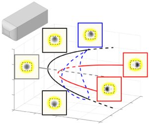
Figure 11. Eigenvalue spectra for the rectangular prism  $W=1.2$, $L=1$, $R=0$, at (a) $Re=185$, between the first and second pitchfork (stationary) bifurcations, and (b) $Re=220$, between the first and second Hopf (oscillating) bifurcations. The first four bifurcating eigenmodes belong to the families $S_y A_z$ and $A_y S_z$, i.e. break either the top/down symmetry or the left/right symmetry, respectively: (c) stationary modes (isosurfaces ${\pm }0.08$ of the streamwise velocity $\hat {{u}}_1$), and (d) oscillatory modes (isosurfaces ${\pm }0.05$ of the real part of the streamwise velocity $\hat {{u}}_1$).
Figures 12(a–d) show the stationary direct and adjoint modes at  $Re=180$. By definition, the $S_y A_z$ mode breaks the top/down symmetry, while the $A_y S_z$ mode breaks the left/right symmetry. Velocity perturbations are maximal in the recirculation region and extend far downstream of the body. Adjoint velocity perturbations are localised in the recirculation region and, to a smaller extent, upstream of the body. This difference in the spatial localisation of direct and adjoint modes is typical of convective non-normality, which results from transport by the base flow in different directions: downstream and upstream for direct and adjoint perturbations, respectively (Chomaz Reference Chomaz2005; Marquet et al. Reference Marquet, Lombardi, Chomaz, Sipp and Jacquin2009). One can also note that the direct modes have a stronger velocity component in the streamwise direction than in the cross-stream directions, while the opposite is true for the adjoint modes. This is analogous to the lift-up type non-normality in parallel shear flows, where cross-stream perturbations (vortices) can generate strong streamwise velocity perturbations (streaks).

Figure 12. (a,b) Stationary direct modes  $\hat {\boldsymbol {u}}_1$, (c,d) adjoint modes $\hat {\boldsymbol {u}}_1^{{\dagger} }$, and (e,f) structural sensitivity $\|\hat {\boldsymbol {u}}_1^{{\dagger} }\|\,\|\hat {\boldsymbol {u}}_1\|$, for the rectangular prism $W=1.2$, $L=1$, $R=0$, at $Re=180$ (between the first and second pitchfork bifurcations), in the planes $z=0$ (top view), $y=0$ (side view) and $x=2.5$ (rear view), for (a,c,e) $S_y A_z$ mode, and (b,d,f) $A_y S_z$ mode.
Figures 12(e,f) show the ‘structural sensitivity’  $\|\hat {\boldsymbol {u}}_1^{{\dagger} }\|\,\|\hat {\boldsymbol {u}}_1\|$ associated with these stationary modes, where $\|{\cdot }\|$ denotes the Euclidean norm. Introduced by Giannetti & Luchini (Reference Giannetti and Luchini2007), the structural sensitivity is an upper bound for the eigenvalue variation $|\delta \lambda |$ induced by a small-amplitude perturbation of the linearised NS operator in the form of a ‘force–velocity coupling’ (i.e. a feedback from a localised velocity sensor to a localised force actuator at the same location). It is maximal where the direct and adjoint modes overlap, and thus identifies the wavemaker region. We note in passing that the sensitivity of an eigenvalue with respect to a base flow modification or to a control can also be computed, at the cost of additional calculations. Here, the structural sensitivity is maximal in the core of the recirculation region, with two main lobes above/below the horizontal plane $z=0$ for the $S_y A_z$ mode, and on the left/right sides of the vertical plane $y=0$ for the $A_y S_z$ mode. Therefore, these two stationary modes are mostly sensitive to localised perturbations in the recirculation region.
Figures 13(a–d) show the (real part of the) oscillatory direct and adjoint modes at  $Re=225$. Direct velocity perturbations extend far downstream of the body, but are maximal farther downstream than for the stationary modes. Adjoint velocity perturbations are localised mainly in the recirculation region, but decrease more slowly upstream up the body than for the stationary modes. Overall, convective non-normality is strong for these two modes as well. Their lift-up type non-normality, however, is weaker than for the stationary modes, as velocity perturbations are less concentrated on one specific component.

Figure 13. Same as figure 12 for the oscillatory (a,b) direct modes  $\hat {\boldsymbol {u}}_1$, (c,d) adjoint modes $\hat {\boldsymbol {u}}_1^{{\dagger} }$, and (e,f) structural sensitivity $\|\hat {\boldsymbol {u}}_1^{{\dagger} }\|\,\|\hat {\boldsymbol {u}}_1\|$, at $Re=225$ (between the first and second Hopf bifurcations). In (a–d), the real part of the complex field is shown.
Figures 13(e,f) show the structural sensitivity associated with these oscillatory modes. Again, it is large in the recirculation region, so these two modes are mostly sensitive to localised perturbations in that region. Unlike the stationary modes, however, the structural sensitivity reaches maximal values along the separation line rather than in the core of the recirculation region.
All the above observations about the stationary/oscillatory direct/adjoint modes and their structural sensitivities are qualitatively very similar to those made by Meliga, Chomaz & Sipp (Reference Meliga, Chomaz and Sipp2009b) for the flow past a sphere. This suggests that despite their non-axisymmetric geometry, rectangular prisms of length-to-height and width-to-height ratios close to 1 share important stability properties with the sphere.
5.1.1. Effect of $L$

In this subsubsection, we investigate the effect of the length  $L$ on the linear stability of wake flows past bodies with sharp edges ( $R=0$). The corresponding steady base flows were described in § 4.2. Figure 14 shows the critical Reynolds number of the first bifurcations observed. Throughout this study, critical Reynolds numbers are computed by cubic interpolation of $Re(\sigma )$ from at least three values of $Re$ that bracket $\sigma =0$, with a maximum step ${\rm \Delta} Re=5$ between two successive Reynolds numbers. For all the values of $L$ investigated in this study, two stationary $S_y A_z$ and $A_y S_z$ modes become unstable first (pitchfork bifurcations), followed by two pairs of oscillatory $S_y A_z$ and $A_y S_z$ modes (Hopf bifurcations). These four bifurcating modes all involve one symmetry breaking, while $S_y S_z$ and $A_y A_z$ modes remain stable until much larger Reynolds numbers. The critical Reynolds numbers of the first four bifurcations shown in figure 14 all increase with $L$. For the flat plate, $L=1/6$, the stationary and oscillatory modes become unstable almost simultaneously, $110 < Re_c < 120$. As $L$ increases, the oscillatory modes remain stable much longer than the stationary ones. Of the two stationary modes, the $S_y A_z$ mode becomes unstable slightly earlier than the $A_y S_z$ mode for $L < 3$, and slightly later for $L > 3$.

Figure 14. Properties of the first bifurcations in the wake flow past rectangular prisms of various lengths  $L$ and with sharp edges ( $R=0$). (a) Critical Reynolds number $Re_c$. Filled symbols indicate stationary (pitchfork) bifurcations; open symbols indicate oscillatory (Hopf) bifurcations. (b) Critical angular frequency $\omega _c=\omega (Re_c)$ (left-hand axis) and Strouhal number $St_c=\omega _c/(2{\rm \pi} )$ (right-hand axis) of the oscillatory modes.
We note that typical oscillatory instabilities in wakes are due to a shear-induced Kelvin–Helmholtz mechanism, implying that global instability occurs when the local growth rate is large enough and the absolutely unstable region is long enough (Chomaz Reference Chomaz2005), such that in 2-D wakes, the critical Reynolds number may be estimated by some measure of the shear or backflow and of the length of the absolutely unstable region (Chiarini, Quadrio & Auteri Reference Chiarini, Quadrio and Auteri2022); by contrast, the physical mechanism responsible for stationary instabilities in 3-D wakes is not fully understood, although some studies did attempt to characterise it (see, for instance, Magnaudet & Mougin (Reference Magnaudet and Mougin2007) on wakes past axisymmetric bubbles). That  $Re_c$ increases with $L$ more slowly for the stationary modes than for the oscillatory modes suggests that the instability mechanisms are associated with different scales, if any.
For all values of  $L$, the two stationary modes become unstable in close succession, which is certainly related to the body width-to-height ratio being close to 1. For thin plates, $L=1/6$, Marquet & Larsson (Reference Marquet and Larsson2015) observed that the gap between the critical Reynolds numbers of these two modes is exactly zero for $W=H$, as expected by symmetry, and increases with $W/H$.
The increase of  $Re_c$ with $L$ is fully consistent with results reported for other 3-D bluff bodies. For example, for axisymmetric bodies such as a thin disk, a sphere and bullet-shaped bodies, the first bifurcating mode is always stationary, followed by an oscillatory mode. As shown in table 1, the associated critical Reynolds numbers increase with the length-to-diameter ratio, $L/D$, and the overall trend is in qualitative agreement with that of the rectangular prisms of the present study (choosing $D$ approximately between the height $H$ and the width $W=1.2H$), including the slower increase of $Re_c$ for larger $L$ values. Note that the first two bifurcating modes reported in table 1 are of azimuthal wavenumber $m=1$ and break the axisymmetry of the wake with an arbitrary azimuthal orientation. By contrast, rectangular prisms have two planar symmetries, which selects the orientation of the modes: vertical wake deflection for modes $S_y A_z$, and lateral deflection for modes $A_y S_z$.
Table 1. Critical Reynolds numbers of the first two bifurcations in wake flows past axisymmetric bodies. Here,  $Re_c^s$ is for stationary (pitchfork) bifurcation, and $Re_c^o$ is for oscillatory (Hopf) bifurcation. All bifurcating modes have an azimuthal wavenumber $m=1$. Ranges reflect variations found in the literature (Natarajan & Acrivos Reference Natarajan and Acrivos1993; Fabre et al. Reference Fabre, Auguste and Magnaudet2008; Gumowski et al. Reference Gumowski, Miedzik, Goujon-Durand, Jenffer and Wesfreid2008; Meliga et al. Reference Meliga, Chomaz and Sipp2009a; Bohorquez et al. Reference Bohorquez, Sanmiguel-Rojas, Sevilla, Jiménez-Gonzáles and Martínez-Bazán2011).

5.1.2. Effect of $R$

We now investigate the effect of the fillet radius  $R$ on the linear stability of wake flows past bodies of length $L=3$, similar to our reference Ahmed body ( $L=3$, $R=0.3472$). The corresponding steady base flows were described in § 4.3. Figure 15(a) shows that for the shorter body, $L=1$, rounding the front edges makes the first four bifurcating modes more stable until $R \simeq 0.1- 0.2$, before making them more unstable. Figure 15(b) shows that for $L=3$, however, rounding makes the stationary modes more unstable. These trends of $Re_c$ are clearly correlated with those of the backflow (figure 9). This is perhaps not surprising for the oscillatory bifurcations, as stronger backflow tends to yield stronger shear. For the stationary bifurcations, it suggests that the instability mechanism is partly related to backflow.

Figure 15. Critical Reynolds number  $Re_c$ of the first stationary bifurcations in the wake flow past rectangular prisms of lengths (a) $L=1$ and (b) $L=3$, and various fillet radii $R$. Filled symbols indicate stationary (pitchfork) bifurcations; open symbols indicate oscillatory (Hopf) bifurcations.
These trends are also similar to those reported in Park & Yang (Reference Park and Yang2016) and Chiarini et al. (Reference Chiarini, Quadrio and Auteri2021) for the first oscillatory mode past 2-D square and rectangular cylinders, respectively. While this may have been anticipated for the oscillatory bifurcations, since the instability mechanism is the same in 2-D and 3-D prism flows, this is not the case for the stationary bifurcations.
6. Weakly nonlinear stability analysis
For the geometries investigated in § 5, two stationary modes, with  $S_y A_z$ and $A_y S_z$ symmetries, are the first to become unstable, and their critical Reynolds numbers are close to one another. In the following, we refer to these modes as modes $A$ and $B$, respectively. Linear stability analysis cannot predict the state of the flow once the two modes are unstable. Therefore, in this section we perform a WNL stability analysis in order to clarify the nonlinear interactions between modes $A$ and $B$, and the nonlinear states expected to be observed in an experiment or DNS close to the bifurcation thresholds. Rigorous WNL analyses based on global eigenmodes have been applied to the first (Hopf) bifurcation of the 2-D circular cylinder wake by Sipp & Lebedev (Reference Sipp and Lebedev2007), and to the first two bifurcations (pitchfork and Hopf) of the axisymmetric disk wake by Meliga et al. (Reference Meliga, Chomaz and Sipp2009a).
Motivated by the strong interest in wake deflection in simplified car models, as already mentioned in § 1, we focus on geometries representative of Ahmed bodies. While the applicability of such a laminar study to practical, turbulent automotive aerodynamics is not straightforward, there is a fundamental interest in understanding the first instabilities and the bifurcation sequence, which may for instance prove useful for flow control, and which also motivated earlier work (Grandemange et al. Reference Grandemange, Cadot and Gohlke2012; Evstafyeva et al. Reference Evstafyeva, Morgans and Dalla Longa2017). We first consider the reference Ahmed body  $W=1.2$, $L=3$, $R=0.3472$, and present detailed WNL results in § 6.2, complemented with DNS results in § 6.3. We will then show in § 6.4 that the WNL bifurcation sequence obtained for this reference geometry is robust to variations in $L$ and $W$ for usual Ahmed body geometries.
6.1. Derivation of the amplitude equations
For the reference Ahmed body, figure 16 shows the eigenspectrum at  $Re=300$, as well as the evolution of the growth rates of modes $A$ and $B$ for Reynolds numbers in the vicinity of $Re=300$. Mode $A$ becomes unstable slightly before mode $B$:
$B$:  $Re_c^A = 293$ and $Re_c^B = 304$. These two modes are depicted in figures 17(a,b), together with the associated adjoint modes in figures 17(c,d). As already observed, mode $A$ breaks the top/down symmetry, while mode $B$ breaks the left/right symmetry. Velocity perturbations extend far downstream and, as expected for stationary modes, do not show the wavepacket structures typical of oscillatory modes. Adjoint perturbations have the same symmetries and are localised in the recirculation region. We note that although eigenmodes are generally complex-valued, stationary modes like modes $A$ and $B$ are associated with real eigenvalues ( $\lambda =\sigma$) and therefore can always be defined as purely real-valued. Figures 17(e,f) show the structural sensitivities of modes $A$ and $B$, which are very similar to those of the two stationary modes in the wake of the shorter prism $L=1$ without fillet (figure 12). Therefore, for the reference Ahmed body too, modes $A$ and $B$ are mostly sensitive to localised perturbations in the recirculation region.

Figure 16. (a) Eigenvalue spectrum for the reference Ahmed body ( $W=1.2$, $L=3$, $R=0.3472$) at $Re=300$, just between the first and second pitchfork bifurcations ( $Re_c^A = 293$, $Re_c^B = 304$). (b) Symbols indicate growth rates of modes $A$ and $B$, the two leading stationary modes. Dashed lines indicate shifted growth rates $\sigma _A-\sigma _A(Re_c)$ and $\sigma _B-\sigma _B(Re_c)$ for $Re_c=300$ (see the WNL analysis in § 6).

Figure 17. Direct modes, adjoint modes and structural sensitivities for the reference Ahmed body ( $W=1.2$, $L=3$, $R=0.3472$) at $Re=300$, in the planes $z=0$ (top view), $y=0$ (side view) and $x=2.5$ (rear view): (a) $\hat {\boldsymbol {u}}_1^A$, (b) $\hat {\boldsymbol {u}}_1^B$, (c) $\hat {\boldsymbol {u}}_1^{A{\dagger} }$, (d) $\hat {\boldsymbol {u}}_1^{B{\dagger} }$, (e) $\|\hat {\boldsymbol {u}}_1^{A{\dagger} }\| \, \|\hat {\boldsymbol {u}}_1^{A}\|$, and (f) $\|\hat {\boldsymbol {u}}_1^{B{\dagger} }\| \, \|\hat {\boldsymbol {u}}_1^{B}\|$.
We assume that the Reynolds number is close to the bifurcation thresholds of modes  $A$ and $B$. We introduce a reference critical Reynolds $Re_c$ that we choose typically in $[Re_c^A, Re_c^B]$, for example $Re_c=300$ for the reference Ahmed body. In practice, the specific choice of $Re_c$ has little effect, as shown in Appendix B. We quantify the departure from criticality with
 \begin{equation} \frac{1}{Re_c} - \frac{1}{Re} = \alpha = \epsilon^2 \tilde\alpha, \end{equation}
where  $0 <\epsilon \ll 1$, and $\tilde \alpha$ is a parameter of order 1 (negative for $Re< Re_c$ and positive for $Re>Re_c$). At $Re_c$, the growth rates $\sigma _A$ and $\sigma _B$ are small but non-zero: mode $A$ is slightly unstable, and mode $B$ is slightly stable (figure 16). Following Meliga et al. (Reference Meliga, Chomaz and Sipp2009a), we introduce rescaled order 1 growth rates
 \begin{equation} \tilde\sigma_A = \frac{\sigma_A}{\epsilon^2},\quad \tilde\sigma_B = \frac{\sigma_B}{\epsilon^2}, \end{equation}
together with a shift operator  $\mathcal {S}$ such that
 \begin{equation} \mathcal{S} \hat{\boldsymbol q}_1^A = \tilde \sigma_A(Re_c)\,\mathcal{B} \hat{\boldsymbol q}_1^A,\quad \mathcal{S} \hat{\boldsymbol q}_1^B = \tilde \sigma_B(Re_c)\,\mathcal{B} \hat{\boldsymbol q}_1^B, \end{equation}
and  $\mathcal {S} \hat {\boldsymbol q}_1 = \boldsymbol 0$ for all other modes. The interest of the shift operator is that although the linearised NS operator is not singular at $Re=Re_c$ (since $\mathcal {A} \hat {\boldsymbol q}_1^A = -\sigma _A \mathcal {B} \hat {\boldsymbol q}_1^A \neq \boldsymbol 0$ and $\mathcal {A} \hat {\boldsymbol q}_1^B = -\sigma _B \mathcal {B} \hat {\boldsymbol q}_1^B \neq \boldsymbol 0$), the shifted linearised NS operator defined by
 \begin{equation} \widetilde{\mathcal{A}} = \mathcal{A} + \epsilon^2 \mathcal{S} \end{equation}
is exactly singular at  $Re=Re_c$ for both modes $A$ and $B$, i.e.
 \begin{equation} \widetilde{\mathcal{A}} \hat{\boldsymbol q}_1^A =\widetilde{\mathcal{A}} \hat{\boldsymbol q}_1^B = \boldsymbol 0. \end{equation}
In other words, modes  $A$ and $B$ are exactly neutral for $\widetilde {\mathcal {A}}$ at $Re=Re_c$, as shown by the shifted growth rates $\sigma _A-\sigma _A(Re_c)$ and $\sigma _B-\sigma _B(Re_c)$ in figure 16.
We perform our WNL analysis with the method of multiple scales, therefore we introduce the slow time scale  $T = \epsilon ^2 t$. The flow field expansion
 \begin{equation} \boldsymbol q(\boldsymbol x,t,T) = \boldsymbol q_0 + \epsilon \boldsymbol q_1+ \epsilon^2 \boldsymbol q_2 + \epsilon^3 \boldsymbol q_3 + \cdots \end{equation}
is injected in the NS equations (5.2) at  $Re=Re_c$, where $\partial _t$ is now transformed into $\partial _t + \epsilon ^2 \partial _T$. Collecting like-order terms in $\epsilon$ and making use of (6.4) yields a series of problems detailed hereafter.
6.1.1. Orders $\epsilon ^0$ and $\epsilon ^1$


The equations at order  $\epsilon ^0$ are the nonlinear NS equations (2.1a,b), and the zeroth-order field $\boldsymbol q_0(\boldsymbol x)$ is the steady base flow computed in § 4 at the reference Reynolds number $Re_c$.
The equations at order  $\epsilon ^1$ are the linearised NS equations (5.3) at $Re=Re_c$, now with the shifted linearised NS operator:
 \begin{equation} \mathcal{B}\,\partial_t {\boldsymbol q}_1 + \widetilde{\mathcal{A}} {\boldsymbol q}_1 = \boldsymbol{0}. \end{equation}
We assume that the first-order field  $\boldsymbol q_1$ is a superposition of the two stationary modes $A$ and $B$ computed in § 5 and shown in figure 17:
 \begin{equation} {\boldsymbol q}_1(\boldsymbol x,T) = A(T)\,\hat{\boldsymbol q}_1^A + B(T)\,\hat{\boldsymbol q}_1^B, \end{equation}
where  $A$ and $B$ are two real-valued slowly varying amplitudes, yet to be determined.
6.1.2. Order $\epsilon ^2$

At order  $\epsilon ^2$, the second-order field $\boldsymbol q_2$ is a solution of the linearised NS equations
 \begin{equation} \mathcal{B}\,\partial_t {\boldsymbol q}_2 + \widetilde{\mathcal{A}} {\boldsymbol q}_2 = (\boldsymbol F_2,0)^{\rm T}, \end{equation}
forced by a term that depends on lower-order fields only,
 \begin{equation} \boldsymbol F_2={-} \tilde\alpha\,\nabla^2 \boldsymbol{u}_0 -(\boldsymbol{u}_1 \boldsymbol{\cdot}\boldsymbol{\nabla}) \boldsymbol{u}_1.\end{equation}
The first term in (6.10) is due to Reynolds number variations (proportional to  $\tilde \alpha$) in the base flow $\boldsymbol {u}_0$, and the second term is due to the transport of $\boldsymbol {u}_1$ by itself. With the expression (6.8) of the first-order field, this forcing reads
 \begin{equation} \boldsymbol F_2 ={-} \tilde\alpha\,\nabla^2 \boldsymbol{u}_0 -A^2 (\hat{\boldsymbol u}_1^A\boldsymbol{\cdot}\boldsymbol{\nabla})\hat{\boldsymbol u}_1^A -B^2 (\hat{\boldsymbol u}_1^B \boldsymbol{\cdot}\boldsymbol{\nabla}) \hat{\boldsymbol u}_1^B -AB \mathcal{C} (\hat{\boldsymbol u}_1^A , \hat{\boldsymbol u}_1^B). \end{equation}
All terms in (6.11) are potentially resonant since they are forcing at zero frequency an operator that is singular precisely at zero frequency, as expressed by (6.5). Considering the spatial symmetries of these terms, however, shows that none of them is resonant, in a manner reminiscent of the cross-junction studied by Bongarzone et al. (Reference Bongarzone, Bertsch, Renaud and Gallaire2021). Indeed,  $\nabla ^2 \boldsymbol {u}_0$, $(\hat {\boldsymbol u}_1^A\boldsymbol {\cdot }\boldsymbol {\nabla })\hat {\boldsymbol u}_1^A$ and $(\hat {\boldsymbol u}_1^B\boldsymbol {\cdot }\boldsymbol {\nabla })\hat {\boldsymbol u}_1^B$ are $S_y S_z$-symmetric, and $(\hat {\boldsymbol u}_1^A \boldsymbol {\cdot }\boldsymbol {\nabla }) \hat {\boldsymbol u}_1^B + (\hat {\boldsymbol u}_1^B \boldsymbol {\cdot }\boldsymbol {\nabla }) \hat {\boldsymbol u}_1^A$ is $A_y A_z$-symmetric, whereas $\widetilde {\mathcal {A}}$ is singular to the $S_y A_z$-symmetric mode $A$ and the $A_y S_z$-symmetric mode $B$. It follows that the forced equation (6.9) can be inverted. We look for a second-order field of the form
 \begin{equation} \boldsymbol{q}_2 (\boldsymbol x, T) = \tilde\alpha \hat{\boldsymbol{q}}_2^{\alpha} + A^2 \hat{\boldsymbol{q}}_2^{A^2} + B^2 \hat{\boldsymbol{q}}_2^{B^2} + AB \hat{\boldsymbol{q}}_2^{AB}, \end{equation}
where each term is the response to the individual forcing terms in (6.11):
 \begin{gather} \mathcal{B}\,\partial_t {\boldsymbol q}_2^\alpha + \widetilde{\mathcal{A}} {\boldsymbol q}_2^\alpha ={-} \tilde\alpha (\nabla^2 \boldsymbol{u}_0, 0)^{\rm T}, \end{gather}
 \begin{gather}\mathcal{B}\,\partial_t {\boldsymbol q}_2^{A^2} + \widetilde{\mathcal{A}} {\boldsymbol q}_2^{A^2} ={-}A^2 ( (\hat{\boldsymbol u}_1^A\boldsymbol{\cdot}\boldsymbol{\nabla})\hat{\boldsymbol u}_1^A, 0)^{\rm T}, \end{gather}
 \begin{gather}\mathcal{B}\,\partial_t {\boldsymbol q}_2^{B^2} + \widetilde{\mathcal{A}} {\boldsymbol q}_2^{B^2} ={-}B^2 ( (\hat{\boldsymbol u}_1^B \boldsymbol{\cdot}\boldsymbol{\nabla}) \hat{\boldsymbol u}_1^B, 0)^{\rm T}, \end{gather}
 \begin{gather}\mathcal{B}\,\partial_t {\boldsymbol q}_2^{AB} + \widetilde{\mathcal{A}} {\boldsymbol q}_2^{AB} ={-}AB (\mathcal{C} (\hat{\boldsymbol u}_1^A , \hat{\boldsymbol u}_1^B), 0)^{\rm T}. \end{gather}
For each of the above problems, boundary conditions are similar to those used for the eigenmodes. In particular, the symmetry of the forcing terms imposes the symmetry of the second-order fields, therefore we use on the symmetry planes the corresponding boundary conditions (5.7) or (5.10). Figure 18 shows the second-order fields. As expected from the symmetries of the forcing terms,  $\boldsymbol u_2^{A^2}$, $\boldsymbol u_2^{B^2}$ and $\boldsymbol u_2^\alpha$ are all doubly symmetric ( $S_y S_z$), while $\boldsymbol u_2^{AB}$ is doubly antisymmetric ( $A_y A_z$).

Figure 18. Second-order fields, shown in the planes  $z=0$ (top view), $y=0$ (side view) and $x=2.5$ (rear view), for (a) $\boldsymbol u_2^{A^2}$, (b) $\boldsymbol u_2^{B^2}$, (c) $\boldsymbol u_2^{AB}$, and (d) $\boldsymbol u_2^\alpha$.
6.1.3. Order $\epsilon ^3$

At order  $\epsilon ^3$, the third-order field $\boldsymbol q_3$ is a solution of the linearised NS equations
 \begin{equation} \mathcal{B}\,\partial_t {\boldsymbol q}_3 + \widetilde{\mathcal{A}} {\boldsymbol q}_3 = (\boldsymbol F_3,0)^{\rm T}, \end{equation}
forced by a term that depends on lower-order fields only,
 \begin{equation} \boldsymbol F_3 ={-}\partial_T \boldsymbol{u}_1 - \tilde\alpha\,\nabla^2 \boldsymbol{u}_1-\mathcal{C}(\boldsymbol{u}_1 , \boldsymbol{u}_2) + \mathcal{S} \boldsymbol{u}_1. \end{equation}
The first term in (6.18) is due to the slow variation of the first-order field  $\boldsymbol {u}_1$, i.e. the yet unknown amplitudes $A(T)$ and $B(T)$. The second term is due to Reynolds number variations in the first-order field $\boldsymbol {u}_1$. The third term is due to the mutual transport of the first- and second-order fields $\boldsymbol {u}_1$ and $\boldsymbol {u}_2$. The last term is due to the non-zero values of the growth rates $\sigma _A$ and $\sigma _B$ at $Re=Re_c$, accounted for by the action of the shift operator. With the expressions (6.8) and (6.12) of the first- and second-order fields, the forcing becomes
 \begin{align} \boldsymbol F_3 &= \left( -\partial_T A - A \tilde\alpha\,\nabla^2 + A \sigma_A \right) \hat{\boldsymbol u}_1^A+ \left(-\partial_T B- B \tilde\alpha\,\nabla^2+ B \sigma_B \right) \hat{\boldsymbol u}_1^B \nonumber\\ &\quad -\mathcal{C}(A \hat{\boldsymbol u}_1^A + B \hat{\boldsymbol u}_1^B, \tilde\alpha \hat{\boldsymbol{u}}_2^{\alpha}+ A^2 \hat{\boldsymbol{u}}_2^{A^2} + B^2 \hat{\boldsymbol{u}}_2^{B^2}+ AB \hat{\boldsymbol{u}}_2^{AB}). \end{align}
It turns out that all terms in (6.19) are either  $S_y A_z$-symmetric or $A_y S_z$-symmetric, and are therefore resonant with mode $A$ or mode $B$. To avoid secular terms, i.e. to ensure that (6.17) can be inverted, a compatibility condition must be enforced. The Fredholm alternative states that the forcing $\boldsymbol {F}_3$ must be orthogonal to the kernel of the adjoint linearised NS operator. This leads to the following equations for the amplitudes $A$ and $B$:
$B$:
 \begin{gather} \partial_t A = \lambda_A A - \chi_A A^3 - \eta_A B^2 A, \end{gather}
 \begin{gather}\partial_t B = \lambda_B B - \chi_B B^3 - \eta_B A^2 B, \end{gather}
where the fast time  $t=T/\epsilon ^2$ has been reintroduced. All the WNL coefficients in (6.20)–(6.21), whose values are reported in Appendix A, are computed as scalar products between the adjoint modes $\hat {\boldsymbol u}_1^{A{\dagger} }$, $\hat {\boldsymbol u}_1^{B{\dagger} }$ and resonant forcing terms:
 \begin{gather} \lambda_A = \epsilon^2 \tilde\lambda_A = \sigma_A -\alpha \langle \hat{\boldsymbol{u}}_1^{A{\dagger}}, \mathcal{C}( \hat{\boldsymbol{u}}_2^\alpha, \hat{\boldsymbol{u}}_1^A) + \nabla^2 \hat{\boldsymbol{u}}_1^A \rangle, \end{gather}
 \begin{gather}\lambda_B = \epsilon^2 \tilde\lambda_B = \sigma_B -\alpha \langle \hat{\boldsymbol{u}}_1^{B{\dagger}}, \mathcal{C}( \hat{\boldsymbol{u}}_2^\alpha, \hat{\boldsymbol{u}}_1^B) + \nabla^2 \hat{\boldsymbol{u}}_1^B \rangle, \end{gather}
 \begin{gather}\eta_A = \epsilon^2 \tilde\eta_A = \epsilon^2 \langle \hat{\boldsymbol{u}}_1^{A{\dagger}}, \mathcal{C}(\hat{\boldsymbol{u}}_2^{B^2}, \hat{\boldsymbol{u}}_1^A) + \mathcal{C}(\hat{\boldsymbol{u}}_2^{AB}, \hat{\boldsymbol{u}}_1^B) \rangle, \end{gather}
 \begin{gather}\eta_B = \epsilon^2 \tilde\eta_B = \epsilon^2 \langle \hat{\boldsymbol{u}}_1^{B{\dagger}}, \mathcal{C}(\hat{\boldsymbol{u}}_2^{A^2}, \hat{\boldsymbol{u}}_1^B) + \mathcal{C}(\hat{\boldsymbol{u}}_2^{AB}, \hat{\boldsymbol{u}}_1^A) \rangle, \end{gather}
 \begin{gather}\chi_A = \epsilon^2 \tilde\chi_A = \epsilon^2 \langle \hat{\boldsymbol{u}}_1^{A{\dagger}}, \mathcal{C}( \hat{\boldsymbol{u}}_2^{A^2} , \hat{\boldsymbol{u}}_1^A ) \rangle, \end{gather}
 \begin{gather}\chi_B = \epsilon^2 \tilde\chi_B = \epsilon^2 \langle \hat{\boldsymbol{u}}_1^{B{\dagger}}, \mathcal{C}(\hat{\boldsymbol{u}}_2^{B^2} , \hat{\boldsymbol{u}}_1^B) \rangle, \end{gather}
where we recall that the adjoint and direct modes are normalised such that  $\langle \hat {\boldsymbol {u}}_1^{A{\dagger} },\ \hat {\boldsymbol {u}}_1^A \rangle = \langle \hat {\boldsymbol {u}}_1^{B{\dagger} },\ \hat {\boldsymbol {u}}_1^B \rangle = 1$.
For any given solution of the amplitude equations (6.20)–(6.21) (see § 6.2), the total flow field up to second order can be reconstructed as
 \begin{equation} \boldsymbol{q} = \boldsymbol q_0 + \epsilon \left(A \hat{\boldsymbol q}_1^A + B \hat{\boldsymbol q}_1^B\right) + \epsilon^2 \left(\tilde\alpha \hat{\boldsymbol{q}}_2^{\alpha} + A^2 \hat{\boldsymbol{q}}_2^{A^2} + B^2 \hat{\boldsymbol{q}}_2^{B^2} + AB \hat{\boldsymbol{q}}_2^{AB}\right)+ O(\epsilon^3). \end{equation}
We note that the values of the WNL coefficients  $\lambda _A, \ldots, \chi _B$, and of the amplitudes $A,B$, depend on the choices of $\epsilon$ and of the direct/adjoint modes normalisation, but the final reconstructed field (6.28) itself is independent of these specific choices.
6.2. Bifurcation diagram
The amplitude equations (6.20)–(6.21) are coupled ordinary differential equations. They are partly similar to the classic Stuart–Landau equation describing the pitchfork/Hopf bifurcation of a single stationary/oscillating mode, but differ by the two nonlinear coupling terms  $\eta _A A B^2$ and $\eta _B B A^2$. Their structure is well known in the literature; see, for instance, Kuznetsov (Reference Kuznetsov2004) for a general mathematical treatment, and Zhu & Gallaire (Reference Zhu and Gallaire2017) and Bongarzone et al. (Reference Bongarzone, Bertsch, Renaud and Gallaire2021) for fluid mechanical examples with two modes, one stationary and one oscillatory, that break two different spatial symmetries. There are in general four equilibrium solutions ( $\partial _t A = \partial _t B = 0$), as follows.
(i) Symmetric state:
$A=B=0$.(ii) Pure state
$A$ (top/down symmetry breaking):
(6.29a,b)\begin{equation} A^2 = \frac{\lambda_A}{\chi_A},\quad B=0. \end{equation}(iii) Pure state
$B$ (left/right symmetry breaking):
(6.30a,b)\begin{equation} A=0,\quad B^2 = \frac{\lambda_B}{\chi_B}. \end{equation}(iv) Mixed state
$(A,B)$ (double symmetry breaking):
(6.31a,b)\begin{equation} A^2 = \frac{\chi_B \lambda_A - \eta_A \lambda_B}{\chi_A \chi_B -\eta_A\eta_B},\quad B^2 = \frac{\chi_A \lambda_B - \eta_B \lambda_A}{\chi_A \chi_B -\eta_A\eta_B}. \end{equation}


We assess the linear stability of each state in two ways: (i) by computing the eigenvalues of the Jacobian  $\boldsymbol{\mathsf{J}}$ of the system linearised about the state of interest,
 \begin{equation} \boldsymbol{\mathsf{J}} = \left[ \begin{array}{cc} \lambda_A - 3 \chi_A A^2 - \eta_A B^2 & - 2 \eta_A B A \\ - 2 \eta_B A B & \lambda_B - 3 \chi_B B^2 - \eta_B A^2 \end{array}\right],\end{equation}
that state being stable if both eigenvalues have a negative real part; (ii) by solving in time the amplitude equations (6.20)–(6.21) from an initial condition close to the state of interest, that state being stable if it is an attractor of the final solution.
We obtain the bifurcation diagram shown in figure 19 for the reference Ahmed body ( $W=1.2$, $L=3$, $R=0.3472$), using $Re_c=300$ and $\epsilon =0.1$. We use a standard representation, where solid lines indicate linearly stable states, and dashed lines indicate unstable states. Pitchfork bifurcations are invariant under reflections $A \rightarrow -A$ and $B \rightarrow -B$, so it is sufficient to report results for $|A|$ and $|B|$ (i.e. for half of the symmetric diagram). The bifurcation sequence is as follows.
(1) For
$Re_c < 293$, only the symmetric base flow is stable.(2) At
$Re = Re_c^A=293$, mode $A$ bifurcates, leading to the stable pure state $(A,0)$ and breaking the top/down symmetry of the base flow.(3) At
$Re = Re_c^B=304$, mode $B$ bifurcates, but the pure state $(0,B)$ is unstable at first, and $(A,0)$ remains the only stable state.(4) At
$Re=314$, the pure state $(0,B)$ becomes stable, thus leading to bistability: either single symmetry-breaking state (top/down or left/right) can be expected to be observed.(5) At
$Re=330$, $(A,0)$ becomes unstable, leaving $(0,B)$ as the only stable state at larger Reynolds numbers.


Figure 19. Bifurcation diagram associated with the amplitude equations (6.20)–(6.21) obtained from a WNL analysis, for the reference Ahmed body ( $W=1.2$, $L=3$, $R=0.3472$), using $Re_c=300$ and $\epsilon =0.1$. Stable and unstable states are shown with solid and dashed lines, respectively. (a) The 3-D view in the $(A,B,Re)$ space. Insets show a rear view of the reconstructed field (see figure 20). (b) The 2-D views in the $(|A|,Re)$ and $(|B|,Re)$ spaces. The shaded region corresponds to bistability and hysteresis.
We note that the mixed state  $(A,B)$ exists in the bistable region but is never stable, meaning that this double symmetry-breaking state is not expected to be observed in a stable manner. Figure 20 shows the four states at $Re=325$, reconstructed up to second order according to (6.28). The wake is deflected clearly in the vertical and horizontal directions in the (stable) pure states $(A,0)$ and $(0,B)$, respectively, and in both directions in the (unstable) mixed state $(A,B)$.

Figure 20. Streamwise velocity  $u$ of reconstructed flows (6.28) at $Re=325$, from the WNL analysis up to second order, shown in the planes $z=0$ (top view), $y=0$ (side view) and $x=2.5$ (rear view), for states (a) $(0,0)$ (unstable), (b) $(A,B)$ (unstable), (c) $(A,0)$ (stable), and (d) $(0,B)$ (stable).
Interestingly, although mode  $A$ bifurcates before mode $B$, state $(A,0)$ quickly becomes unstable, and eventually $(0,B)$ remains the only stable state. In other words, the top/down symmetry-breaking state cannot be observed except in the range $293 \leq Re \leq 330$, while the left/right symmetry-breaking state can be observed for $Re \geq 316$. This is precisely the same symmetry breaking as that observed in the turbulent regime, where Ahmed body wakes deflect along the longer dimension of the body. Therefore, unlike wakes past 2-D cylinders and 3-D disks, spheres and bullet-shaped axisymmetric bluff bodies, the preferred turbulent symmetry breaking in the Ahmed body wake is reminiscent not of the first laminar bifurcation, but of the second one. Our WNL analysis rationalises this observation by unveiling the bifurcation sequence. In § 6.4, we will demonstrate the robustness of this sequence for other geometries typical of Ahmed bodies.
6.3. Comparison with DNS
In this subsection, we perform fully nonlinear DNS of the flow past our reference Ahmed body ( $W=1.2$, $L=3$, $R=0.3472$) at various Reynolds numbers, with the aim of confirming the bifurcation sequence obtained in § 6.2. In particular, we investigate whether the single symmetry-breaking states $(A,0)$ and $(0,B)$ are indeed observed, and if they appear and disappear in the same order. We also look for evidence of bistability and hysteresis, increasing and decreasing the Reynolds number in two independent sequences: $Re=290 \rightarrow 310 \rightarrow 330$, etc., and $Re=410 \rightarrow 390 \rightarrow 370$, etc. In each case, simulations are run for a sufficiently long time to allow the flow to reach a truly stationary state. We determine the flow state by monitoring the horizontal velocity $v(x,0,0)$ and the vertical velocity $w(x,0,0)$ on the symmetry axis. Specifically, we should obtain:
(i)
$v=w=0$ for the symmetric base flow;(ii)
$v=0$, $w\neq 0$ for the top/down symmetry-breaking state $(A,0)$;(iii)
$v\neq 0$, $w=0$ for the left/right symmetry-breaking state $(0,B)$;(iv)
$v\neq 0$, $w\neq 0$ for the double symmetry-breaking state $(A,B)$, although we do not expect to observe this state in the stationary regime.


Figure 21 shows the velocities obtained in the stationary regime at the location  $(x^*,0,0) = (2.5,0,0)$. In all simulations, the final flow is steady, without any oscillations. When increasing $Re$, the vertical velocity $w$ first becomes non-zero when $Re \simeq 300$, while $v=0$. In other words, state $(A,0)$ is observed. This state loses stability when $Re \simeq 340$, and the flow shifts to state $(0,B)$, with a non-zero horizontal velocity $v$, while $w=0$, for this and larger Reynolds numbers. When decreasing $Re$, state $(0,B)$ persists until $Re \simeq 320$, at which point the flow shifts back to state $(A,0)$. Therefore, this suggests hysteresis in the approximate range of Reynolds numbers $[315 \pm 10, 340 \pm 10]$.

Figure 21. Vertical and horizontal velocities in the wake in  $(x^*,0,0) = (2.5,0,0)$, obtained from DNS of the reference Ahmed body ( $W=1.2$, $L=3$, $R=0.3472$). Upward-pointing symbols ( $\vartriangle$) correspond to increasing Reynolds numbers, and downward-pointing symbols ( $\triangledown$) correspond to decreasing Reynolds numbers. The shaded region shows bistability and hysteresis.
It is worth mentioning that the flow transitions between  $(A,0)$ and $(0,B)$ via a state reminiscent of the double symmetry-breaking state $(A,B)$ (rather than via the symmetric base flow), although this state is visited only transiently. We also note that transitions are rather slow (of the order of $10^3$ convective time units), consistent with the small growth rates of the Jacobian (6.32) calculated near the corresponding transitions, i.e. near the boundaries between stages 3 and 4, and between stages 4 and 5, in the bifurcation diagram of figure 19.
The qualitative agreement between DNS and WNL analysis is excellent for the transition Reynolds numbers between stages 1, 2 and 3. At larger  $Re$, the agreement deteriorates for the transition Reynolds numbers between stages 3, 4 and 5, which may be ascribed to the increasing departure from criticality. Nonetheless, the whole bifurcation sequence is well predicted by the WNL analysis.
As a concluding remark, we note that since the two bifurcations of interest are stationary, it would also be possible to compute the fully nonlinear states with a continuation method or, alternatively, with the self-consistent model proposed by Camarri & Mengali (Reference Camarri and Mengali2019).
6.4. Effect of $W$ and $L$


We have presented the bifurcation diagram of our reference Ahmed body ( $W=1.2$, $L=3$, $R=0.3472$) in § 6.2. One may wonder whether this sequence is robust to geometric modifications. Indeed, Ahmed bodies studied in the literature show some variations in dimension, especially in width and length (table 2). Therefore we investigate the effect of $W$ and $L$, keeping the fillet radius constant ( $R=0.3472$). Specifically, we consider narrower and wider bodies ( $W \in [1, 1.35]$, $L=3$), as well as shorter and longer bodies ( $W=1.2$, $L \in [2.6, 3.8]$). We compute the base flow and eigenmodes for these bodies, and determine the critical Reynolds numbers $Re_c^A$ and $Re_c^B$. We then set $Re_c$ by rounding $(Re_c^A+Re_c^B)/2$ to the nearest multiple of 5, and finally we compute the coefficients of the amplitude equations (6.20)–(6.21).
Table 2. Typical Ahmed body widths and lengths (normalised by the body height) found in the literature.

A convenient way to summarise the results is to consider the different possible bifurcation diagrams for this type of amplitude equation. As detailed in Kuznetsov (Reference Kuznetsov2004), there are five topologically different bifurcation diagrams, corresponding to different regions of the  $\theta$– $\delta$ plane, where $\theta$ and $\delta$ are mixed ratios of the nonlinear coefficients of (6.20)–(6.21):
 \begin{equation} \theta = \frac{\eta_A}{\chi_B},\quad \delta = \frac{\eta_B}{\chi_A}. \end{equation}
Figure 22(a) shows the five regions, labelled I to V, for the case  $\theta \geq \delta$ relevant here. As will soon become clear, regions I ( $\theta >0$, $\delta >0$, $\theta \delta >1$) and II ( $\theta >0$, $\delta >0$, $\theta \delta <1$) are of particular interest to our study. In region I, the bifurcation diagram is as sketched in figure 23(a), and is topologically equivalent to that obtained in § 6.2. We recall briefly the bifurcation sequence for increasing $Re$:
$Re$:
(1) only the trivial state
$(0,0)$ is stable;(2) mode
$A$ bifurcates and the stable state $(A,0)$ appears;(3) mode
$B$ bifurcates and the unstable state $(0,B)$ appears;(4) state
$(B,0)$ becomes stable and the unstable mixed state $(A,B)$ appears;(5) state
$(A,B)$ disappears and state $(A,0)$ becomes unstable – only $(0,B)$ remains stable.


Figure 22. (a) Five regions of the  $\theta$– $\delta$ plane, associated with the five possible bifurcation diagrams for the amplitude equations (6.20)–(6.21). (b) Variation of $\theta$ and $\delta$ with $W$ and $L$ for rectangular prisms of fixed fillet radius $R=0.3472$. Dashed lines are a guide to the eye. In the considered range of widths $1 \leq W \leq 1.35$, and lengths $2.6 \leq L \leq 3.8$, representative of most Ahmed bodies, $\theta$ and $\delta$ stay in region I, i.e. the bifurcation diagram remains as in figures 19 and 23(a).

Figure 23. Schematic bifurcation diagrams in (a) region I and (b) region II of the  $\theta$– $\delta$ plane of figure 22. Stable and unstable states are shown with solid and dashed lines, respectively. (c) Corresponding phase portraits in the $A$–
$A$– $B$ amplitude plane. Stable and unstable states are shown with filled and open symbols, respectively. Dashed arrows in stage 4 show how the mixed state $(A,B)$ moves with $Re$.
$Re$.
In the neighbouring region II, the bifurcation diagram is as sketched in figure 23(b), and corresponds to another bifurcation sequence:
(1) only the trivial state
$(0,0)$ is stable;(2) mode
$A$ bifurcates and the stable state $(A,0)$ appears;(3) mode
$B$ bifurcates and the unstable state $(0,B)$ appears;(4) state
$(A,0)$ becomes unstable and the stable mixed state $(A,B)$ appears;(5) state
$(A,B)$ disappears and state $(0,B)$ becomes stable.


Although the initial stages (1–3) and the final stage (5) are identical in regions I and II, what happens in between (stage 4, shaded region in figure 23a) is fundamentally different: in region I the pure states  $(A,0)$ and $(B,0)$ are simultaneously stable (bistability) while the mixed state $(A,B)$ cannot be observed; by contrast, in region II the pure states $(A,0)$ and $(B,0)$ are unstable and only the mixed state $(A,B)$ can be observed. This is also apparent in the phase portraits of figure 23(c). From stages 3 to 5, the stability of the pure states $(A,0)$ and $(0,B)$ is exchanged. In region I, this happens as the unstable mixed state $(A,B)$ is born in $(0,B)$ (making it stable) and dies when colliding with $(A,0)$ (making it unstable). In region II, the stable mixed state $(A,B)$ is born in $(A,0)$ (making it unstable) and dies when colliding with $(0,B)$ (making it stable).
Figure 22(b) shows that all the Ahmed bodies considered in this study fall in region I of the  $\theta$– $\delta$ plane. Our reference Ahmed body corresponds to $\theta = 2.68$, $\delta =0.554$ (filled symbol). The effect of $L$ is very limited, with $\theta$ and $\delta$ barely varying compared to their reference values (inset). The effect of $W$ is much more significant, with $\theta$ and $\delta$ varying substantially: the point $(\theta,\delta )$ moves away from the boundary between regions I and II as the body becomes wider, and vice versa. By symmetry, the limiting case $W=1$ (body as wide as tall, seldom used in practice for Ahmed bodies) lies exactly on the boundary. We can conclude that in the WNL framework, the bifurcation sequence obtained in § 6.2 is robust to width and length variations commonly encountered for Ahmed bodies.
One must keep in mind that the WNL analysis is rigorously valid in the vicinity of  $Re_c$ only. Therefore, one cannot completely rule out a fully nonlinear bifurcation diagram that differs from the WNL one, e.g. an incursion in region II. More generally, it is likely that the deflected wake undergoes one or several secondary instabilities at sufficiently large Reynolds number. Nonetheless, the fact that stages 1–3 and 5 are identical in regions I and II suggests that the transition from state $(A,0)$ to state $(0,B)$ is, in any case, a robust feature of this flow. Furthermore, the fully nonlinear DNS bifurcation sequence (§ 6.3) is in very good agreement with the WNL prediction for the reference Ahmed body, which attests to the reliability of the WNL analysis.
7. Conclusion
In this study, we have investigated the stability of 3-D rectangular prism wakes of width-to-height ratio  $W/H=1.2$. Linear stability analysis showed that two stationary modes become unstable via pitchfork bifurcations, at critical Reynolds numbers close to one another. Mode $A$ breaks the top/down planar symmetry, and mode $B$ the left/right planar symmetry. At larger $Re$, two oscillatory modes become unstable via Hopf bifurcations, each mode breaking either planar symmetry. The critical Reynolds numbers all increase with the body length $L$, similar to the pitchfork and Hopf bifurcations of axisymmetric wakes. The effect of the leading edge fillet radius $R$ is limited, and depends on $L$.
$L$.
Next, a weakly nonlinear analysis performed in the vicinity of the critical  $Re$ of modes $A$ and $B$ yielded a set of two coupled amplitude equations. For Ahmed bodies, the bifurcation diagram revealed that the flow first undergoes a stationary bifurcation leading to a wake deflection in the top/down direction, or state $(A,0)$. Then another stationary state $(0,B)$ with the opposite symmetry breaking, i.e. in the left/right direction, becomes stable. Simultaneously, a double symmetry-breaking state $(A,B)$ appears but remains unstable at all $Re$. The two single symmetry-breaking states thus coexist in a range of Reynolds numbers. Finally, state $(A,0)$ becomes unstable, leaving state $(0,B)$ as the only stable state. The corresponding wake deflection, i.e. along the larger dimension of the body, is the same as the static deflection observed in the turbulent wakes of Ahmed bodies, with or without ground proximity.
Fully nonlinear DNS confirmed the whole bifurcation sequence, including bistability-induced hysteresis, and the final  $(0,B)$ state. We also demonstrated that the bifurcation sequence was robust to variations in body width $W$ and body length $L$ in the range of common Ahmed body geometries.
Natural extensions of this work may include: (i) sensitivity analysis with respect to control, in order to determine optimal control strategies and locations; (ii) analysis of possible secondary instabilities at larger  $Re$, especially along the $(0,B)$ branch; and (iii) analysis of the linear and weakly nonlinear stability of Ahmed bodies with modifications suppressing one of the two planar symmetries, such as ground proximity, yaw/pitch angles, and asymmetric body geometries.
Acknowledgements
E.B. thanks O. Cadot for stimulating discussions about Ahmed bodies and symmetry breaking, E. Yim for initial versions of the base flow and linear stability codes, A. Gimmonet for his work in the initial stage of this study, and Scitas for support with EPFL's high-performance computing clusters. Useful comments from A. Bongarzone and F. Gallaire about the weakly nonlinear analysis are also acknowledged.
Funding
G.A.Z. acknowledges the financial support of the Swiss National Science Foundation (grant no. P_Z00P_2_193180).
Declaration of interests
The authors report no conflict of interest.
Author contributions
G.A.Z. performed the DNS and wrote the paper. E.B. conceived the study, performed the linear stability and weakly nonlinear analyses, and wrote the paper.
Appendix A. Numerical domain and mesh
All FreeFEM calculations (base flow, linear stability, WNL analysis) are performed on the quarter-space domain  $\varOmega ' = \{ x,y,z \, | \, {-10} \leq x \leq 20,\ 0 \leq y,\ z \leq 10 \}$. Mesh points are strongly clustered near the body, with density 1 on the outermost boundaries, 10 on the boundaries of the sub-domain $\{ x,y,z \, | \, {-5} \leq x \leq 15,\ 0 \leq y,\ z \leq 2 \}$, and $n$ on the body surface. Table 3 reports the variation with $n$ of several quantities: base drag coefficient and recirculation length at $Re=300$, growth rates of modes $A$ and $B$ at $Re=300$, critical Reynolds number of modes $A$ and $B$, and WNL coefficients for $Re_c=300$. Increasing $n$ from 40 to 80, thus doubling the number of elements $N_{{elmts}}$ and degrees of freedom $N_{{DOF}}$, leads to reasonably small variations of all the quantities of interest. Throughout the study, we have used mesh M2. Similarly, table 4 reports variations with the domain size. The drag coefficient, recirculation length and critical Reynolds numbers are all well converged. The WNL coefficients (and therefore the amplitudes) do show some variation, but not the ratios $\theta$ and $\delta$, which implies that the bifurcation diagram is consistently predicted to be topologically as in region I.
Table 3. Influence of the mesh size on several properties of the base flow, linear stability analysis and weakly nonlinear analysis (WNL), for the reference Ahmed body ( $W=1.2$, $L=3$, $R=0.3472$). The drag coefficient $C_D$, recirculation length $L_r$ and eigenvalues $\sigma ^A,\sigma ^B$ are calculated at $Re=300$. The WNL coefficients are computed with the reference Reynolds number $Re_c=300$.

Table 4. Influence of the domain size on several properties of the base flow, linear stability analysis and WNL analysis, for the reference Ahmed body ( $W=1.2$, $L=3$, $R=0.3472$). The drag coefficient $C_D$, recirculation length $L_r$ and eigenvalues $\sigma ^A,\sigma ^B$ are calculated at $Re=300$. The WNL coefficients are computed with the reference Reynolds number $Re_c=300$.

Appendix B. Effect of the reference Reynolds number on the bifurcation diagram
Figure 24 shows the bifurcation diagram obtained with different choices of the reference Reynolds number,  $Re_c=295$, 300 and 305, close to the first two pitchfork bifurcations ( $Re_c^A=293$ and $Re_c^B=304$). We observe no significant effect on the bifurcation sequence, i.e. on the symmetry-breaking states, their stability and amplitudes. The onset of existence of states $(A,0)$ and $(0,B)$ is not modified either. Only the extent of the bistability region is slightly modified as $Re_c$ increases: the lower bound varies between $Re=312$ and 316, and the upper bound between $Re=328$ and 331.

Figure 24. Effect of the reference Reynolds number on the bifurcation diagram, for the reference Ahmed body ( $W=1.2$, $L=3$, $R=0.3472$): arrows show increasing values $Re_c=295$, 300, 305.


 Open access