Hostname: page-component-788cddb947-m6qld Total loading time: 0 Render date: 2024-10-10T02:12:27.509Z Has data issue: false hasContentIssue false

A high-order asymptotic analysis of the Benjamin–Feir instability spectrum in arbitrary depth

Published online by Cambridge University Press:  08 February 2023

Ryan P. Creedon*
Affiliation:
Department of Applied Mathematics, University of Washington, Seattle, WA USA
Bernard Deconinck*
Affiliation:
Department of Applied Mathematics, University of Washington, Seattle, WA, USA
*
Email addresses for correspondence: creedon@uw.edu, deconinc@uw.edu

Abstract

We investigate the Benjamin–Feir (or modulational) instability of Stokes waves, i.e. small-amplitude, one-dimensional periodic gravity waves of permanent form and constant velocity, in water of finite and infinite depth. We develop a perturbation method to describe to high-order accuracy the unstable spectral elements associated with this instability, obtained by linearizing Euler's equations about the small-amplitude Stokes waves. These unstable elements form a figure-eight curve centred at the origin of the complex spectral plane, which is parametrized by a Floquet exponent. Our asymptotic expansions of this figure-eight are in excellent agreement with numerical computations as well as recent rigorous results by Berti et al. (Full description of Benjamin–Feir instability of Stokes waves in deep water, 2021, arXiv:2109.11852) and Berti et al. (Benjamin–Feir instability of Stokes waves in finite depth, 2022, arXiv:2204.00809). From our expansions, we derive high-order estimates for the growth rates of the Benjamin–Feir instability and for the parametrization of the Benjamin–Feir figure-eight curve with respect to the Floquet exponent. We are also able to compare the Benjamin–Feir and high-frequency instability spectra analytically for the first time, revealing three different regimes of the Stokes waves, depending on the predominant instability.

Type
JFM Papers
Copyright
© The Author(s), 2023. Published by Cambridge University Press

1. Introduction

Stokes (Reference Stokes1847) derived a formal asymptotic expansion for the small-amplitude, periodic travelling wave solutions of the full water wave equations in infinite depth, see figure 1 for a schematic. Seventy-five years later, Nekrasov (Reference Nekrasov1921) and Levi-Civita (Reference Levi-Civita1925) proved the validity of these expansions if the amplitude $\varepsilon$ of the waves is sufficiently small. Not long after, Struik (Reference Struik1926) extended this analysis to finite depth. The stability with respect to sideband perturbations of these solutions, now known as Stokes waves, was investigated first experimentally by Benjamin & Feir (Reference Benjamin and Feir1967) and immediately after supported by independent formal calculations by Benjamin (Reference Benjamin1967) and Whitham (Reference Whitham1967) using distinct methods. Both calculations suggest that Stokes waves are modulationally unstable with respect to longitudinal sideband perturbations provided $\kappa h > \alpha _{BW}$, where $\kappa$ is the wavenumber of the Stokes waves, $h$ is the constant depth of the water and $\alpha _{BW} = 1.3627827567\ldots$. This instability is now known as the Benjamin–Feir or modulational instability.

Figure 1. Schematic of a $2{\rm \pi} /\kappa$-periodic Stokes wave $\eta _S$ in finite depth $h$. The wave travels uniformly to the left or right, depending on its velocity. In the case of infinite depth, Stokes derived an asymptotic expansion for $\eta _S$ and its velocity as power series in a small parameter $\varepsilon$ related to the amplitude of the wave.

In the years since the pioneering work of Benjamin and Whitham, several papers have explored the Benjamin–Feir instability experimentally, numerically and analytically. It is impossible to summarize all these works here, rather we highlight a few works that are most relevant to our investigation. For a more comprehensive history of the Benjamin–Feir instability, see Craik (Reference Craik2004), Grimshaw (Reference Grimshaw2005), Yuen & Lake (Reference Yuen and Lake1980) and, in different contexts, Deconinck & Oliveras (Reference Deconinck and Oliveras2011), Korotkevich, Dyachenko & Zakharov (Reference Korotkevich, Dyachenko and Zakharov2016) and Zakharov & Ostrovsky (Reference Zakharov and Ostrovsky2009).

Beginning in the 1970s, Bryant (Reference Bryant1974, Reference Bryant1978) numerically studied the stability of Stokes waves in shallow water ($\kappa h<\alpha _{BW}$) with respect to co-periodic longitudinal and transverse perturbations, respectively. Around the same time, Longuet-Higgins (Reference Longuet-Higgins1978a,Reference Longuet-Higginsb) used similar numerical methods to study the stability of Stokes waves with respect to sub- and super-harmonic longitudinal perturbations in infinitely deep water. McLean (Reference McLean1982) generalized the numerical results of Bryant and Longuet-Higgins by investigating the stability of Stokes waves in finite depth with respect to sub- and super-harmonic transverse perturbations.

The results of Bryant and Longuet-Higgins are obtained by perturbing the Stokes waves $\eta _S$ in a co-moving frame according to

(1.1)\begin{equation} \eta(x,t;\varepsilon,\rho) = \eta_S(x;\varepsilon) + \rho \exp({\lambda t + {\rm i} \mu x}) \mathcal{N}(x) + {O}(\rho^2), \end{equation}

where $x$ is the horizontal coordinate in the co-moving frame, $\rho$ is a small parameter unrelated to the amplitude of the Stokes wave $\varepsilon$, $\lambda \in \mathbb {C}$ controls the exponential growth rates of the perturbation, $\mu \in (-\kappa /2,\kappa /2]$ is called the Floquet exponent and determines the periodic (or quasi-period) of the perturbation, and $\mathcal {N}(x)$ is a sufficiently smooth, $2{\rm \pi} /\kappa$-periodic function. The results of McLean are obtained if dependence on a transverse variable $y$ is introduced appropriately in (1.1).

Substituting (1.1) into the full water wave equations and linearizing in $\rho$ leads to a family of spectral problems parametrized by the Floquet exponent $\mu$ for fixed wave amplitude $\varepsilon$. The eigenvalues of each spectral problem are given by the exponential growth rates $\lambda$ in (1.1) and their corresponding eigenfunctions are $\mathcal {N}(x)$ (Kapitula & Promislow Reference Kapitula and Promislow2013). The union of these eigenvalues over $\mu \in (-\kappa /2,\kappa /2]$ yields a continuous spectrum called the stability spectrum of the Stokes wave. The Benjamin–Feir instability occurs when four eigenvalues with the same Floquet exponent collide at the origin of the stability spectrum and separate, each eigenvalue occupying a distinct quadrant, as the amplitude $\varepsilon$ of the Stokes wave increases. This is a consequence of the quadrafold symmetry of the spectrum due to the Hamiltonian structure of the water wave equations (Zakharov Reference Zakharov1968; Haragus & Kapitula Reference Haragus and Kapitula2008).

Despite numerical evidence of these eigenvalues close to the origin in the stability spectrum, a proof of their existence did not appear until 1995. In the classic work of Bridges & Mielke (Reference Bridges and Mielke1995), techniques from spatial dynamics and centre manifold theory are used to prove the existence of unstable eigenvalues close to the origin whenever $\kappa h > \alpha _{BW}$ and $\varepsilon$ is sufficiently small. The proof is valid for any finite depth but fails in water of infinite depth. Only in the past two years have Nguyen & Strauss (Reference Nguyen and Strauss2020) developed a proof based on Lyapunov–Schmidt reduction that works in both finite and infinite depth. Another proof based on periodic Evans functions appeared in the literature more recently (Hur & Yang Reference Hur and Yang2022).

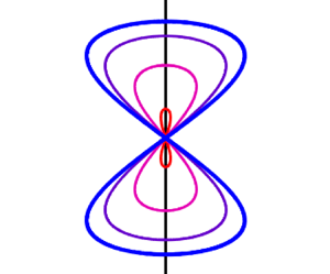
In 2011, Deconinck & Oliveras (Reference Deconinck and Oliveras2011) revisited the numerical computations of McLean and others but allowed for more generic choices of the Floquet exponent $\mu$ (Deconinck & Kutz Reference Deconinck and Kutz2006). To our knowledge, this is the first work displaying full stability spectra of Stokes waves in finite and infinite depth that exhibits a figure-eight curve at the origin of the complex spectral plane associated with the Benjamin–Feir instability, see a schematic in figure 2. Evidence of instabilities away from the origin, referred to as high-frequency instabilities, was also demonstrated by Deconinck & Oliveras (Reference Deconinck and Oliveras2011). These high-frequency instabilities have been analytically explored with Trichtchenko in Creedon, Deconinck & Trichtchenko (Reference Creedon, Deconinck and Trichtchenko2022) and by Hur & Yang (Reference Hur and Yang2022).

Figure 2. Schematic of the stability spectrum for a small-amplitude Stokes wave in sufficiently deep water. Spectral elements with positive real part indicate instability according to (1.1). The Benjamin–Feir figure-eight curve is coloured blue, while the high-frequency instabilities are coloured orange. In this manuscript, we are concerned with high-order asymptotic approximations of the blue figure-eight curve. For the corresponding approximations of the high-frequency instabilities in orange, see Creedon et al. (Reference Creedon, Deconinck and Trichtchenko2022).

In recent months, seminal work by Berti, Maspero & Ventura (Reference Berti, Maspero and Ventura2021, Reference Berti, Maspero and Ventura2022) has confirmed the existence of the Benjamin–Feir figure-eight in finite and infinite depth, provided $\kappa h > \alpha _{BW}$ and $\varepsilon$ is sufficiently small. The proof of both cases relies on the Hamiltonian and reversibility properties of the water wave equations together with Kato's theory of similarity transformations (Kato Reference Kato1966) and KAM theory. Reported in these works are explicit expressions for the figure-eight curves, up to real analytic functions of the Floquet exponent $\mu$ and the amplitude of the Stokes waves $\varepsilon$. A low-order approximation of the curves is also given.

In this work, we obtain high-order asymptotic expansions of the Benjamin–Feir figure-eight curve in finite and infinite depth. In particular, we seek high-order asymptotic estimates for the interval of Floquet exponents parametrizing the figure-eight and for the most unstable eigenvalue. Using the results of Creedon et al. (Reference Creedon, Deconinck and Trichtchenko2022) allows us to compare the Benjamin–Feir and high-frequency growth rates analytically. This comparison suggests three regimes for Stokes waves: (i) shallow water ($\kappa h < \alpha _{BW}$), in which only high-frequency instabilities exist; (ii) intermediate water ($\alpha _{BW}<\kappa h<\alpha _{DO}(\varepsilon ) = 1.4308061674\ldots +{O}(\varepsilon ^2)$), in which both instabilities exist but high-frequency instabilities dominate; and (iii) deep water ($\kappa h > \alpha _{DO}(\varepsilon )$), in which both instabilities are present, but the Benjamin–Feir instability dominates.

Our method to obtain these high-order asymptotic approximations is a modification of that developed for high-frequency instabilities in Creedon, Deconinck & Trichtchenko (Reference Creedon, Deconinck and Trichtchenko2021a,Reference Creedon, Deconinck and Trichtchenkob) and Creedon et al. (Reference Creedon, Deconinck and Trichtchenko2022). Although the method is formal, it offers a more direct approach to the Benjamin–Feir figure-eight curve and produces results consistent with numerical computations (for sufficiently small $\varepsilon$) as well as with rigorous results reported by Berti et al. (Reference Berti, Maspero and Ventura2021, Reference Berti, Maspero and Ventura2022). The method loses validity for sufficiently large $\varepsilon$, when the Benjamin–Feir instability spectrum separates from the origin and changes its topology, see figure 3. Some of the lower-order details of our method are also presented by Akers (Reference Akers2015) for the Benjamin–Feir instability in infinite depth, although this work uses different conventions for the water wave equations and underlying Stokes waves. In contrast, our expressions are in one-to-one correspondence with those reported by Berti et al. (Reference Berti, Maspero and Ventura2021, Reference Berti, Maspero and Ventura2022), giving confidence in the rigorous results as well as in our asymptotic calculations.

Figure 3. Numerically computed Benjamin–Feir instability spectra in infinitely deep water for Stokes waves of amplitude $\varepsilon = 0.31$ (a), $\varepsilon = 0.32$ (b), and $\varepsilon = 0.33$ (c). The methods presented in this work apply only for sufficiently small $\varepsilon$ and, thus, do not capture the separation of the figure-eight from the origin.

2. Preliminaries

2.1. AFM formulation of the water wave equations

The Euler equations governing the dynamics of a one-dimensional periodic water wave free of surface tension over an inviscid, irrotational and two-dimensional bulk are

(2.1a)$$\begin{gather} \phi_{xx} + \phi_{zz} = 0, \quad \text{in} \ \{(x,z):|x|<{\rm \pi}/\kappa\ \text{and}\ -h < z < \eta \}, \end{gather}$$
(2.1b)$$\begin{gather}\eta_t + \eta_x \phi_x = \phi_z, \quad \text{on} \ z=\eta, \end{gather}$$
(2.1c)$$\begin{gather}\phi_t + \frac{1}{2} (\phi_x^2 + \phi_z^2) + g\eta = 0, \quad \text{on} \ z=\eta, \end{gather}$$
(2.1d)$$\begin{gather}\phi_z = 0, \quad \text{on} \ z={-}h, \end{gather}$$

together with the periodicity conditions

(2.2a)$$\begin{gather} \eta(-{\rm \pi}/\kappa,t) = \eta({\rm \pi}/\kappa,t), \end{gather}$$
(2.2b)$$\begin{gather}\phi_x(-{\rm \pi}/\kappa,z,t) = \phi_x({\rm \pi}/\kappa,z,t), \quad \phi_z(-{\rm \pi}/\kappa,z,t) = \phi_z({\rm \pi}/\kappa,z,t). \end{gather}$$

Here, $x$ is the horizontal coordinate, $z$ is the vertical coordinate, $t$ is time, $\eta (x,t)$ is the surface profile of the water wave relative to the $z=0$ reference level, $\phi (x,z,t)$ is the velocity potential in the bulk, $g$ is the magnitude of the vertical acceleration due to gravity, $h$ is the average depth of the water (assuming constant bathymetry) and $2{\rm \pi} /\kappa$ is the period of the wave.

Many formulations of water waves exist that avoid the bulk variable $\phi$ but whose dynamics are fully equivalent to (2.1)–(2.2), e.g. Craig & Sulem (Reference Craig and Sulem1993), Dyachenko, Zakharov & Kuznetsov (Reference Dyachenko, Zakharov and Kuznetsov1996), Shaw (Reference Shaw1979) and Zakharov (Reference Zakharov1968). We use the Ablowitz–Fokas–Musslimani (AFM) formulation (Ablowitz, Fokas & Musslimani Reference Ablowitz, Fokas and Musslimani2006; Ablowitz & Haut Reference Ablowitz and Haut2008), which only involves the surface variables $\eta$ and $q = \phi (x,\eta,t)$ and avoids computations of the Dirichlet-to-Neumann operator. The AFM equations can be written as

(2.3a)$$\begin{gather} \int_{-{\rm \pi}/\kappa}^{{\rm \pi}/\kappa} {\rm e}^{-{\rm i}\kappa m x}\left[\eta_t\cosh\left(\kappa m\left(\eta + h\right) \right) +{\rm i}q_x\sinh\left(\kappa m\left(\eta + h \right) \right) \right] {\rm d}\kern0.7pt x= 0, \quad m \in \mathbb{Z} \setminus \{0\}, \end{gather}$$
(2.3b)$$\begin{gather}q_t + \frac12 q_x^2 +g\eta - \frac{1}{2}\frac{\left(\eta_t +\eta_xq_x\right)^2}{1+\eta_x^2} = 0. \end{gather}$$

Throughout this work, we refer to (2.3a) and (2.3b) as the non-local and local equations, respectively.

Moving to a travelling frame $x \rightarrow x -ct$ with velocity $c$ and rescaling variables as in Creedon et al. (Reference Creedon, Deconinck and Trichtchenko2022), one arrives at the non-dimensional AFM equations

(2.4a)$$\begin{gather} \int_{-{\rm \pi}}^{\rm \pi} {\rm e}^{-{\rm i} m x}\left[\left(\eta_t-c\eta_x\right)\cosh\left( m\left(\eta + \alpha\right) \right) +{\rm i}q_x\sinh\left(m\left(\eta + \alpha \right) \right) \right] \,{{\rm d}\kern0.7pt x} = 0, \quad m \in \mathbb{Z} \setminus \{0\}, \end{gather}$$
(2.4b)$$\begin{gather}q_t - cq_x + \frac12 q_x^2 +\eta - \frac{1}{2}\frac{\left(\eta_t-c\eta_x +\eta_xq_x\right)^2}{1+\eta_x^2} = 0, \end{gather}$$

where $\alpha = \kappa h$ is the aspect ratio of the depth of the water to the period of the surface waves modulo $2{\rm \pi}$. These non-dimensionalized equations are equivalent to the dimensional equations ((2.3a) and (2.3b)) in the travelling frame with $\kappa = 1$ and $g=1$.

Remark 2.1 In infinitely deep water, the local equation (2.4b) is unchanged while the non-local equation (2.4a) becomes

(2.5)\begin{equation} \int_{-{\rm \pi}}^{\rm \pi} \exp({-{\rm i} m x +|m|\eta}) \left[|m|\left(\eta_t-c\eta_x\right) + {\rm i} m q_x \right] \,{{\rm d}\kern0.7pt x} = 0, \quad m \in \mathbb{Z} \setminus \{0\}. \end{equation}

2.2. Small-amplitude Stokes waves

We seek time-independent solutions $\eta _S = \eta _S(x)$ and $q_S= q_S(x)$ of (2.4a) and (2.4b) that satisfy:

  1. (i) $\eta _S$ and $q_S$ are infinitely differentiable with respect to $x$;

  2. (ii) $\eta _S$ and $q_{S,x}$ are $2{\rm \pi}$-periodic with respect to $x$, where $q_{S,x}$ represents the $x$-derivative of $q_S$;

  3. (iii) $\eta _S$, $q_{S,x}$ and $c$ depend analytically on a small parameter $\varepsilon$ such that

    (2.6)\begin{equation} \eta_S|_{\varepsilon =0} = 0 = q_{S,x}|_{\varepsilon =0} \quad \text{and} \quad \|\eta_S\|_{{L}^2} = \varepsilon + {O}(\varepsilon^2) \quad \text{as}\ \varepsilon \rightarrow 0; \end{equation}
  4. (iv) $\eta _S$ and $q_{S,x}$ are even in $x$ without loss of generality and $c(\varepsilon )$ is even in $\varepsilon$; and

  5. (v) $\eta _S$ has zero average.

These solutions correspond to the small-amplitude Stokes waves discussed in § 1. Their existence is proven by Levi-Civita (Reference Levi-Civita1925), Nekrasov (Reference Nekrasov1921) and Struik (Reference Struik1926). Expansions of $\eta _S$, $q_S$ and $c$ as power series in $\varepsilon$ are carried out by Creedon et al. (Reference Creedon, Deconinck and Trichtchenko2022) using the AFM equations (2.4a) and (2.4b). These expansions take the form

(2.7a)$$\begin{gather} \eta_S(x;\varepsilon) = \varepsilon\cos(x) + \sum_{j=2}^{\infty} \eta_j(x)\varepsilon^j, \end{gather}$$
(2.7b)$$\begin{gather}q_S(x;\varepsilon) = \frac{\varepsilon}{c_0}\sin(x)+ \sum_{j=2}^{\infty} q_j(x)\varepsilon^j, \end{gather}$$
(2.7c)$$\begin{gather}c(\varepsilon) = c_0 + \sum_{j=1}^{\infty} c_{2j}\varepsilon^{2j}, \end{gather}$$

where $c_0^2 = \tanh (\alpha )$. In what follows, we study right-travelling waves so that $c_0=\sqrt {\tanh (\alpha )}>0$.

The higher-order corrections of $\eta _S$ and $q_S$ (for $j>1$) take the form

(2.8a)$$\begin{gather} \eta_{j}(x) = \begin{cases} \displaystyle \sum_{\substack{\ell = 2 \\ \ell\ \text{even}}}^{j}\hat{N}_{j,\ell}\cos(\ell x) & \text{for}\ j\ \text{even}, \\ \displaystyle \sum_{\substack{\ell = 3 \\ \ell\ \text{odd}}}^{j}\hat{N}_{j,\ell}\cos(\ell x) & \text{for}\ j\ \text{odd}, \end{cases} \end{gather}$$
(2.8b)$$\begin{gather}q_{j}(x) = \begin{cases} \displaystyle \hat{Q}_{j,0}x+\sum_{\substack{\ell = 2 \\ \ell\ \text{even}}}^{j}\hat{Q}_{j,\ell}\sin(\ell x) & \text{for}\ j\ \text{even}, \\ \displaystyle \sum_{\substack{\ell = 3 \\ \ell\ \text{odd}}}^{j}\hat{Q}_{j,\ell}\sin(\ell x) & \text{for}\ j\ \text{odd}, \end{cases} \end{gather}$$

where $\hat {N}_{j,\ell }$ and $\hat {Q}_{j,\ell }$ depend only on the aspect ratio $\alpha$. Explicit representations of these coefficients as well as those for $c$ are provided in Creedon et al. (Reference Creedon, Deconinck and Trichtchenko2022) to ${O}(\varepsilon ^4)$. Taking their limits as $\alpha \rightarrow \infty$ gives the corresponding coefficients in infinite depth.

Remark 2.2 The expansion of $q_S$ contains terms proportional to $x$ due to the induced mean flow of the travelling frame, so $q_S$ is not periodic in general. Despite this, $q_{S,x}$ is periodic, which implies that the horizontal velocity at the surface is periodic.

Remark 2.3 From our properties of Stokes waves above, we implicitly define the small-amplitude parameter $\varepsilon$ as the first Fourier cosine mode of $\eta _S$. Other authors, e.g. Whitham (Reference Whitham1974), may use a different convention for this parameter and, as a result, derive seemingly different asymptotic expansions of the Stokes waves. Up to redefining the small-amplitude parameter, however, the expansions are equivalent.

2.3. Stability spectrum of Stokes waves

Extending our periodic domain to the whole real line, we perturb the Stokes waves using

(2.9)\begin{equation} \begin{pmatrix} \eta(x,t;\varepsilon,\rho) \\ q(x,t;\varepsilon,\rho) \end{pmatrix} = \begin{pmatrix} \eta_S(x;\varepsilon) \\ q_S(x;\varepsilon) \end{pmatrix} + \rho \begin{pmatrix} \eta_\rho(x,t) \\ q_\rho(x,t) \end{pmatrix} + {O}\left(\rho^2\right), \end{equation}

where $|\rho |\ll 1$ is a parameter independent of $\varepsilon$, and $\eta _\rho$ and $q_\rho$ are sufficiently smooth functions of $x$ and $t$ that are bounded over the real line for each $t\geq 0$. If (2.9) satisfies the AFM equations to ${O}(\rho )$, then, after separating time and space variables and using Floquet–Bloch theory (Deconinck & Oliveras Reference Deconinck and Oliveras2011; Creedon et al. Reference Creedon, Deconinck and Trichtchenko2022), the perturbations applied to the Stokes waves must take the form

(2.10)\begin{equation} \begin{pmatrix} \eta_{\rho}(x,t) \\ q_{\rho}(x,t) \end{pmatrix} = \exp({\lambda t+{\rm i}\mu x})\begin{pmatrix} \mathcal{N}(x) \\ \mathcal{Q}(x) \end{pmatrix} + {\rm c.c.}, \end{equation}

where ${\rm c.c.}$ denotes the complex conjugate of what precedes, $\mu \in (-1/2,1/2]$ is the Floquet exponent and ${\boldsymbol w} = (\mathcal {N},\mathcal {Q})^{\rm T}$ is a sufficiently smooth, $2{\rm \pi}$-periodic eigenfunction of the spectral problem

(2.11)\begin{equation} \mathcal{L}_{\mu,\varepsilon}{\boldsymbol w}(x) = \lambda\mathcal{R}_{\mu,\varepsilon}{\boldsymbol w}(x), \end{equation}

with corresponding eigenvalue $\lambda \in \mathbb {C}$. In general, the linear operators $\mathcal {L}_{\mu,\varepsilon }$ and $\mathcal {R}_{\mu,\varepsilon }$ depend nonlinearly on $\varepsilon$ and $\mu$. Explicitly,

(2.12a,b)\begin{equation} \mathcal{L}_{\mu,\varepsilon} = \begin{pmatrix} \mathcal{L}_{\mu,\varepsilon}^{(1,1)} & \mathcal{L}_{\mu,\varepsilon}^{(1,2)} \\ \mathcal{L}_{\mu,\varepsilon}^{(2,1)} & \mathcal{L}_{\mu,\varepsilon}^{(2,2)} \end{pmatrix}, \quad \mathcal{R}_{\mu,\varepsilon} = \begin{pmatrix} \mathcal{R}_{\mu,\varepsilon}^{(1,1)} & 0 \\ \mathcal{R}_{\mu,\varepsilon}^{(2,1)} & 1 \end{pmatrix}, \end{equation}
(2.13a)$$\begin{gather} \mathcal{L}_{\mu,\varepsilon}^{(1,1)}[\mathcal{N}(x)] \,{=}\, \sum_{n={-}\infty}^{\infty}{\rm e}^{{\rm i}nx} \mathcal{F}_n \left[c\, \mathcal{C}_{n+\mu}\mathcal{D}_x\mathcal{N}(x) \,{+}\,(n+\mu)\left(c\,\mathcal{S}_{n+\mu}\eta_{S,x}\,{-}\,{\rm i}\mathcal{C}_{n+\mu}q_{S,x} \right)\mathcal{N}(x)\right], \end{gather}$$
(2.13b)$$\begin{gather}\mathcal{L}_{\mu,\varepsilon}^{(1,2)}[\mathcal{Q}(x)] = \sum_{n={-}\infty}^{\infty}{\rm e}^{{\rm i}nx}\mathcal{F}_n\left[-{\rm i}\mathcal{S}_{n+\mu}\mathcal{D}_x\mathcal{Q}(x) \right], \end{gather}$$
(2.13c)$$\begin{gather}\mathcal{L}_{\mu,\varepsilon}^{(2,1)}[\mathcal{N}(x)] = \eta_{S,x}{\zeta}^2\mathcal{D}_x\mathcal{N}(x) - \mathcal{N}(x), \end{gather}$$
(2.13d)$$\begin{gather}\mathcal{L}_{\mu,\varepsilon}^{(2,2)}[\mathcal{Q}(x)] ={-}{\zeta}\mathcal{D}_x\mathcal{Q}(x), \end{gather}$$
(2.13e)$$\begin{gather}\mathcal{R}_{\mu,\varepsilon}^{(1,1)}[\mathcal{N}(x)] = \sum_{n={-}\infty}^{\infty}{\rm e}^{{\rm i}nx}\mathcal{F}_n\left[\mathcal{C}_{n+\mu}\mathcal{N}(x) \right], \end{gather}$$
(2.13f)$$\begin{gather}\mathcal{R}_{\mu,\varepsilon}^{(2,1)}[\mathcal{N}(x)] ={-}\eta_{S,x}{\zeta}\mathcal{N}(x), \end{gather}$$

where $\eta _{S,x}$ represents the $x$-derivative of $\eta _S$,

(2.14ad)\begin{equation} \mathcal{C}_k = \cosh(k(\eta_S+\alpha)), \quad \mathcal{S}_k = \sinh(k(\eta_S+\alpha)), \quad \mathcal{D}_x = {\rm i}\mu+\partial_x, \quad {\zeta} =\frac{q_{S,x}- c}{1+\eta_{S,x}^2}, \end{equation}

and

(2.15)\begin{equation} \mathcal{F}_n[f(x)] = \frac{1}{2{\rm \pi}}\int_{-{\rm \pi}}^{\rm \pi} {\rm e}^{-{\rm i}nx} f(x) \,{{\rm d}\kern0.7pt x}, \end{equation}

for any $f(x) \in \text {L}^2_{per}(-{\rm \pi},{\rm \pi} )$. The eigenvalues $\lambda \in \mathbb {C}$ of (2.11) correspond to the exponential growth rates of the perturbations $\eta _{\rho }$ and $q_{\rho }$. Consequently, we define the stability spectrum of a Stokes wave with amplitude $\varepsilon$ as the union of these eigenvalues over $\mu \in (-1/2,1/2]$.

Remark 2.4 The eigenvalues of (2.11) for fixed $\mu \in (-1/2,0)$ are conjugate to the eigenvalues with Floquet exponent $-\mu$, so we may restrict $\mu \in [0,1/2]$ without loss of generality.

Remark 2.5 In infinite depth,

(2.16a)$$\begin{gather} \mathcal{L}_{\mu,\varepsilon}^{(1,1)}[\mathcal{N}(x)] = \sum_{n={-}\infty}^{\infty}\, {\rm e}^{{\rm i}nx}\mathcal{F}_n\left[{\rm e}^{|n+\mu|\eta_S}|n+\mu|\left(c\mathcal{D}_x\mathcal{N}(x)\right.\right.\nonumber\\ \left.\left. + \left(c\eta_{S,x}|n+\mu|-{\rm i}(n+\mu)q_{S,x}\right)\mathcal{N}(x) \right) \right], \end{gather}$$
(2.16b)$$\begin{gather}\mathcal{L}_{\mu,\varepsilon}^{(1,2)}[\mathcal{Q}(x)] = \sum_{n={-}\infty}^{\infty} {\rm e}^{{\rm i}nx}\mathcal{F}_n\left[{\rm e}^{|n+\mu| \eta_S}\left(-{\rm i}(n+\mu)\mathcal{D}_x\mathcal{Q}(x) \right)\right], \end{gather}$$
(2.16c)$$\begin{gather}\mathcal{R}_{\mu,\varepsilon}^{(1,1)}[\mathcal{N}(x)] = \sum_{n={-}\infty}^{\infty} {\rm e}^{{\rm i}nx}\mathcal{F}_n\left[{\rm e}^{|n+\mu|\eta_S}|n+\mu|\mathcal{N}(x)\right]. \end{gather}$$

All other operators remain the same as above.

For generic choices of $\varepsilon$ and $\mu$, the spectral problem (2.11) can only be solved numerically, see Deconinck & Oliveras (Reference Deconinck and Oliveras2011), for example. However, in the special case $\varepsilon = 0$, (2.11) reduces to a constant-coefficient problem,

(2.17)$$\begin{gather} \begin{pmatrix} {\rm i}c_0(\mu+D)\cosh(\alpha(\mu+D)) & (\mu+D)\sinh(\alpha(\mu+D)) \\ -1 & {\rm i}c_0(\mu+D) \end{pmatrix} {\boldsymbol w_0}(x) \nonumber\\ = \lambda_0\begin{pmatrix} \cosh(\alpha(\mu+D)) & 0 \\ 0 & 1 \end{pmatrix}{\boldsymbol w_0}(x), \end{gather}$$

with $D=-{\rm i}\partial _x$. We solve (2.17) to find

(2.18)\begin{equation} \lambda_{0} ={-}{\rm i}\varOmega_{\sigma}(\mu+n), \quad \sigma ={\pm} 1, \quad n \in \mathbb{Z},\end{equation}

for

(2.19)\begin{equation} \varOmega_{\sigma}(k) ={-}c_0k +\sigma \omega(k), \quad \omega(k) = \text{sgn}(k)\sqrt{k\tanh(\alpha k)}. \end{equation}

Equation (2.19) is the linear dispersion relation of the non-dimensional AFM equations in a frame travelling at velocity $c_0$. The parameter $\sigma$ specifies the branch of this dispersion relation. Since both branches are real-valued, all eigenvalues $\lambda _0$ are imaginary and the zero-amplitude Stokes waves are spectrally stable.

For almost all $\mu$ and $n$, (2.18) is a simple eigenvalue with one-dimensional eigenspace spanned by

(2.20)\begin{equation} {\boldsymbol w_0}(x) = \begin{pmatrix} 1 \\ \dfrac{-{\rm i}\sigma}{\omega(\mu+n)} \end{pmatrix}{\rm e}^{{\rm i}nx}. \end{equation}

For $\lambda _0$ to enter the right-half plane and give rise to an instability for $0<\varepsilon \ll 1$, it must be non-simple. That is, at least two eigenvalues must collide at $\lambda _0$ for the eigenvalues to leave the imaginary axis (MacKay & Saffman Reference MacKay and Saffman1986; Deconinck & Trichtchenko Reference Deconinck and Trichtchenko2017). There are a countably infinite number of pairs $(\mu,n)$ for which this occurs (Creedon et al. Reference Creedon, Deconinck and Trichtchenko2021a). Most of these pairs correspond to eigenvalues away from the origin in the complex spectral plane that generate high-frequency instabilities for $0<\varepsilon \ll 1$ (Deconinck & Trichtchenko Reference Deconinck and Trichtchenko2017; Creedon et al. Reference Creedon, Deconinck and Trichtchenko2022; Hur & Yang Reference Hur and Yang2022). The pairs $(0,-1)$, $(0,0)$ and $(0,1)$, however, correspond to the eigenvalue at the origin. This eigenvalue generates the Benjamin–Feir instability in sufficiently deep water for $0 < \varepsilon \ll 1$ (Bridges & Mielke Reference Bridges and Mielke1995; Hur & Yang Reference Hur and Yang2022; Nguyen & Strauss Reference Nguyen and Strauss2020; Berti et al. Reference Berti, Maspero and Ventura2021, Reference Berti, Maspero and Ventura2022).

Remark 2.6 In infinite depth, (2.17) becomes

(2.21)\begin{equation} \begin{pmatrix}{\rm i}c_0(\mu+D)|\mu+D| & (\mu+D)^2 \\ -1 & {\rm i}c_0(\mu+D) \end{pmatrix} {\boldsymbol w_0}(x) = \lambda_0\begin{pmatrix} |\mu+D| & 0 \\ 0 & 1 \end{pmatrix}{\boldsymbol w_0}(x). \end{equation}

The corresponding eigenvalues take the form of (2.18) with

(2.22)\begin{equation} \varOmega_{\sigma}(k) ={-}c_0k +\sigma \omega(k), \quad \omega(k) = {\rm sgn}(k)\sqrt{|k|}. \end{equation}

2.4. A spectral perturbation method for the Benjamin–Feir instability

To reveal the structure in our perturbation calculations, we denote the zero eigenvalue of the $\varepsilon = 0$ spectrum and its corresponding zero Floquet exponent by $\lambda _0$ and $\mu _0$, respectively. However, since $\lambda _0 = 0$ and $\mu _0 = 0$, one can omit these parameters in what follows.

The eigenvalue $\lambda _0$ is non-simple with algebraic multiplicity 4 and geometric multiplicity 3 (Bridges & Mielke Reference Bridges and Mielke1995; Nguyen & Strauss Reference Nguyen and Strauss2020; Berti et al. Reference Berti, Maspero and Ventura2021, Reference Berti, Maspero and Ventura2022; Hur & Yang Reference Hur and Yang2022). The corresponding eigenspace is spanned by

(2.23ac)\begin{equation} {\boldsymbol w_{0,-1}}(x) = \begin{pmatrix} 1 \\ {\rm i}/c_0 \end{pmatrix}{\rm e}^{-{\rm i}x}, \quad {\boldsymbol w_{0,0}}(x) = \begin{pmatrix} 0 \\ 1 \end{pmatrix}, \quad {\boldsymbol w_{0,1}}(x) = \begin{pmatrix} 1 \\ -{\rm i}/c_0 \end{pmatrix}{\rm e}^{{\rm i}x}. \end{equation}

The most general eigenfunction corresponding to $\lambda _0$ is therefore

(2.24)\begin{equation} {\boldsymbol w_0}(x) = \beta_{0,-1}{\boldsymbol w_{0,-1}}(x) + \beta_{0,0}{\boldsymbol w_{0,0}}(x) + \beta_{0,1}{\boldsymbol w_{0,1}}(x), \end{equation}

where $\beta _{0,\nu }$ for $\nu \in \{0,\pm 1\}$ are (for now) arbitrary constants. This eigenfunction gives the leading-order behaviour of the spatial dependence of the perturbation applied to the Stokes waves.

Remark 2.7 The generalized eigenspace is spanned by (2.21) together with the generalized eigenvector ${\boldsymbol v_{0,0}} = (1,0)^{\rm T}$. We mention this for completeness, but in practice, we only need (2.23ac) to approximate the unstable eigenvalues corresponding to the Benjamin–Feir instability.

Remark 2.8 Without loss of generality, one of the constants $\beta _{0,\nu }$ can be set to 1 since ${\boldsymbol w}_0$ is unique only up to a non-zero scalar. We retain all three constants in our calculations for reasons that become clearer when we consider infinite depth.

We turn on the $\varepsilon$ parameter and track the unstable eigenvalues near the origin for $0 < \varepsilon \ll 1$. These eigenvalues trace out a figure-eight curve centred at the origin, as mentioned in § 1. To track these eigenvalues and their corresponding eigenfunctions, we formally expand in powers of $\varepsilon$:

(2.25a)$$\begin{gather} \lambda(\varepsilon)= \lambda_0 + \sum_{j=1}^{\infty}\lambda_j \varepsilon^j, \end{gather}$$
(2.25b)$$\begin{gather}{\boldsymbol w}(x;\varepsilon) = {\boldsymbol w_0}(x) + \sum_{j=1}^{\infty}{\boldsymbol w_j}(x) \varepsilon^j. \end{gather}$$

As the curve deforms with $\varepsilon$, so too does its parametrization in terms of the Floquet exponent. Hence, as in Creedon et al. (Reference Creedon, Deconinck and Trichtchenko2022), we expand this parameter as well, writing

(2.26)\begin{equation} \mu(\varepsilon) = \mu_0+\varepsilon\mu_1\left(1+r(\varepsilon)\right), \quad \text{with}\ r(\varepsilon) = \sum_{j=1}^{\infty}r_j\varepsilon^j, \end{equation}

where $\mu _1$ assumes an interval of values symmetric approximately zero and $r(\varepsilon )$ captures the higher-order deformations of this interval, see figure 4.

Remark 2.9 For sufficiently large $\varepsilon$, the figure-eight curve separates from the origin (figure 3), and thus, the parametrizing interval of Floquet exponents separates into two disjoint intervals. Ansatz (2.26) cannot account for this effect, which limits our analysis of the Benjamin–Feir instability spectrum to sufficiently small $\varepsilon$.

Figure 4. Schematic of the parametrizing interval of Floquet exponents for the Benjamin–Feir figure-eight curve as a function of $\varepsilon$. The grey-shaded region indicates the leading-order approximation of this interval $\varepsilon \mu _1$, where $\mu _1$ is an interval of values symmetric approximately zero. The blue-shaded region indicates the true interval as a function of $\varepsilon$ and is a uniform rescaling of the leading-order behaviour by a factor of $1+r(\varepsilon )$, where $r$ is an analytic function of $\varepsilon$ such that $r(\varepsilon ) = o(1)$ as $\varepsilon \searrow 0$. The boundaries of the true interval may be subtended by curves that are concave up or down, depending on $\alpha$.

We proceed as follows. Expansions (2.25a), (2.25b) and (2.26) are substituted into the full spectral problem (2.11). Powers of $\varepsilon$ are equated, generating a hierarchy of linear inhomogeneous equations for the eigenfunction corrections ${\boldsymbol w_j}$. Each of these equations is solvable only if the Fredholm alternative removes secular inhomogeneous terms. This leads to a set of solvability conditions that impose constraints on the eigenvalue corrections $\lambda _j$ as well as corrections to the constants appearing in ${\boldsymbol w_0}$. Corrections to the Floquet exponent require an additional constraint called the regular curve condition (Creedon et al. Reference Creedon, Deconinck and Trichtchenko2021a,Reference Creedon, Deconinck and Trichtchenkob, Reference Creedon, Deconinck and Trichtchenko2022), which ensures the eigenvalue corrections remain bounded as one approaches the intersection of the figure-eight curve with the imaginary axis.

We present this method in more detail in the sections that follow, first in finite depth and then in infinite depth, where more care is needed. Results of the method are compared directly with numerical computations of the Benjamin–Feir instability using methods presented by Deconinck & Kutz (Reference Deconinck and Kutz2006) and Deconinck & Oliveras (Reference Deconinck and Oliveras2011). To our knowledge, this is the first time that analytical and numerical descriptions of the Benjamin–Feir figure-eight curve have been quantitatively compared.

3. The Benjamin–Feir spectrum in finite depth

3.1. The ${O}(\varepsilon )$ problem

Substituting (2.25a), (2.25b) and (2.26) into the full spectral problem (2.11), terms of ${O}(\varepsilon ^0)$ necessarily cancel by our choice of $\lambda _0$, ${\boldsymbol w_0}$ and $\mu _0$ above. At ${O}(\varepsilon )$, we find

(3.1)\begin{equation} \left(\mathcal{L}_0 - \lambda_0\mathcal{R}_0\right){\boldsymbol w_1} ={-}\mathcal{L}_1{\boldsymbol w_0} + \mathcal{R}_0\left(\lambda_1{\boldsymbol w_0} \right) + \mathcal{R}_1\left(\lambda_0{\boldsymbol w_0} \right), \end{equation}

with

(3.2a,b)\begin{equation} \mathcal{L}_j = \frac{1}{j!}\frac{\partial^j}{\partial \varepsilon^j} \mathcal{L}_{\mu(\varepsilon),\varepsilon}, \quad \mathcal{R}_j = \frac{1}{j!}\frac{\partial^j}{\partial \varepsilon^j} \mathcal{R}_{\mu(\varepsilon),\varepsilon}. \end{equation}

The operator $\mathcal {L}_0-\lambda _0\mathcal {R}_0$ is not invertible for $(\lambda _0, \mu _0)=(0,0)$. A solution ${\boldsymbol w_1}$ of (3.1) exists only if the inhomogeneous terms are orthogonal to the nullspace of the adjoint of $\mathcal {L}_0-\lambda _{0}\mathcal {R}_0$ by the Fredholm alternative. A direct calculation shows

(3.3) \begin{equation} \text{Null}((\mathcal{L}_0-\lambda_{0}\mathcal{R}_0)^{\dagger}) = \text{Span}\left\{ \begin{pmatrix} 1 \\ {\rm i}c_0 \end{pmatrix} {\rm e}^{-{\rm i}x}, \begin{pmatrix} 1 \\ 0 \end{pmatrix},\begin{pmatrix} 1 \\ -{\rm i}c_0 \end{pmatrix} {\rm e}^{{\rm i}x} \right\}, \end{equation}

where $(\mathcal {L}_0-\lambda _{0}\mathcal {R}_0)^{{\dagger} }$ denotes the adjoint operator with respect to the standard complex inner-product $\left \langle {\cdot },{\cdot }\right \rangle$ on $\text {L}^2_{per}(-{\rm \pi},{\rm \pi} )\times \text {L}^2_{per}(-{\rm \pi},{\rm \pi} )$. From (3.3), we arrive at three solvability conditions for (3.1):

(3.4a)$$\begin{gather} \left\langle -\mathcal{L}_1{\boldsymbol w_0} + \mathcal{R}_0\left(\lambda_1{\boldsymbol w_0} \right) + \mathcal{R}_1\left(\lambda_0{\boldsymbol w_0} \right),\begin{pmatrix} 1 \\ {\rm i}c_0 \end{pmatrix} {\rm e}^{-{\rm i}x}\right\rangle = 0, \end{gather}$$
(3.4b)$$\begin{gather}\left\langle -\mathcal{L}_1{\boldsymbol w_0} + \mathcal{R}_0\left(\lambda_1{\boldsymbol w_0} \right) + \mathcal{R}_1\left(\lambda_0{\boldsymbol w_0} \right),\begin{pmatrix} 1 \\ 0 \end{pmatrix}\right\rangle = 0, \end{gather}$$
(3.4c)$$\begin{gather}\left\langle -\mathcal{L}_1{\boldsymbol w_0} + \mathcal{R}_0\left(\lambda_1{\boldsymbol w_0} \right) + \mathcal{R}_1\left(\lambda_0{\boldsymbol w_0} \right),\begin{pmatrix} 1 \\ -{\rm i}c_0 \end{pmatrix} {\rm e}^{{\rm i}x} \right\rangle = 0. \end{gather}$$

Simplifying (3.4a) and (3.4c) leads to

(3.5a)$$\begin{gather} 2\beta_{0,-1}\left(\lambda_1 + {\rm i}\mu_1c_g\right) = 0, \end{gather}$$
(3.5b)$$\begin{gather}2\beta_{0,1}\left(\lambda_1+{\rm i}\mu_1c_g\right) = 0, \end{gather}$$

respectively, where $c_g$ denotes the group velocity of $\varOmega _{1}$ (2.19) evaluated at $k=1$. Explicitly,

(3.6)\begin{equation} c_g = \frac{\alpha(1-c_0^4)-c_0^2}{2c_0}. \end{equation}

In contrast to (3.4a) and (3.4c), (3.4b) reduces to a trivial equality and does not contribute an additional solvability condition.

Remark 3.1 If $c_0>0$, a direct calculation shows that $c_g<0$ for $\alpha >0$.

If we require $\beta _{0,\nu } \neq 0$ so that the eigenspace of $\lambda _0$ remains three-dimensional, (3.5a) and (3.5b) imply

(3.7)\begin{equation} \lambda_1 ={-}{\rm i}\mu_1c_g. \end{equation}

Since $\mu _1 \in \mathbb {R}$, the unstable eigenvalues of the Benjamin–Feir instability are imaginary to ${O}(\varepsilon )$.

Remark 3.2 If $\beta _{0,\nu } = 0$ for some $\nu$, one recovers the imaginary spectrum near the origin, as opposed to the figure-eight curve.

Before proceeding to ${O}(\varepsilon ^2 )$, we solve (3.1) subject to (3.7). The solution ${\boldsymbol w_1}$ decomposes into a direct sum of a particular solution ${\boldsymbol w_{1,p}}$ and a homogeneous solution ${\boldsymbol w_{1,h}}$:

(3.8)\begin{equation} {\boldsymbol w_1}(x) = {\boldsymbol w_{1,p}}(x)+{\boldsymbol w_{1,h}}(x). \end{equation}

The particular solution can be written as

(3.9)\begin{equation} {\boldsymbol w_{1,p}}(x) = \sum_{j={-}2}^{2} {\boldsymbol w_{1,j}}{\rm e}^{{\rm i}jx}, \end{equation}

where ${\boldsymbol w_{1,j}} = {\boldsymbol w_{1,j}}(\alpha,\beta _{0,\nu },\mu _1)\in \mathbb {C}^2$. The homogeneous solution is

(3.10)\begin{equation} {\boldsymbol w_{1,h}}(x) = \beta_{1,-1}{\boldsymbol w_{0,-1}}(x) + \beta_{1,0}{\boldsymbol w_{0,0}}(x) + \beta_{1,1}{\boldsymbol w_{0,1}}(x), \end{equation}

coinciding with the eigenspace of $\lambda _0$. The coefficients $\beta _{1,\nu }$ represent first-order corrections to the zeroth-order eigenfunction correction ${\boldsymbol w}_0$ and are undetermined constants at this order.

Remark 3.3 The expressions for ${\boldsymbol w_{1,j}}$ as well as for all other algebraic expressions that are too cumbersome to include explicitly in this manuscript are found in our companion Mathematica files available at https://doi.org/10.1017/jfm.2022.1031.

3.2. The ${O}(\varepsilon ^2)$ problem

At ${O}(\varepsilon ^2)$, the spectral problem (2.11) takes the form

(3.11)\begin{align} \left(\mathcal{L}_0 - \lambda_0\mathcal{R}_0\right){\boldsymbol w_2} ={-}\sum_{j=1}^{2}\mathcal{L}_j{\boldsymbol w_{2-j}} + \mathcal{R}_0\left(\sum_{k=1}^{2}\lambda_k{\boldsymbol w_{2-k}} \right) + \sum_{j=1}^{2}\mathcal{R}_j\left(\sum_{k=0}^{2-j} \lambda_{k}{\boldsymbol w_{2-j-k}} \right). \end{align}

Proceeding as above, we obtain three non-trivial solvability conditions for (3.11):

(3.12a)$$\begin{gather} 2\beta_{0,-1}\left(\lambda_2 + {\rm i}c_gr_1\mu_1 \right) + \beta_{0,0}S_{2,-1}\mu_1 + {\rm i}(U_{2,-1}\beta_{0,1} + (T_{2,-1}\mu_1^2 + V_{2,-1} )\beta_{0,-1} ) = 0, \end{gather}$$
(3.12b)$$\begin{gather}\beta_{0,0}T_{2,0}\mu_1^2 + {\rm i}S_{2,0}\mu_1(\beta_{0,-1}+\beta_{0,1}) = 0 , \end{gather}$$
(3.12c)$$\begin{gather}2\beta_{0,1}(\lambda_2+{\rm i}c_gr_1\mu_1)+\beta_{0,0}S_{2,1}\mu_1 + {\rm i}(U_{2,1}\beta_{0,-1} + (T_{2,1}\mu_1^2+V_{2,1})\beta_{0,1}) = 0 , \end{gather}$$

where the subscripted coefficients $S$, $T$, $U$ and $V$ are all real-valued functions of the aspect ratio $\alpha$. More explicitly, we have

(3.13a)$$\begin{gather} S_{2,-1} = \frac{\alpha+5c_0^2-2\alpha c_0^4-c_0^6+\alpha c_0^8}{4c_0^2}, \end{gather}$$
(3.13b)$$\begin{gather}T_{2,-1} = \frac{\alpha^2-c_0^2\left({-}1+\alpha c_0^2 \right)\left({-}2\alpha +c_0^2+3\alpha c_0^4 \right)}{4c_0^3}, \end{gather}$$
(3.13c)$$\begin{gather}U_{2,-1} = \frac{1-2\hat{N}_{2,2}c_0^2\left(1-3c_0^4\right)-8\hat{Q}_{2,2}c_0^3-4c_0^4+c_0^8}{4c_0^3}, \end{gather}$$
(3.13d)$$\begin{gather}T_{2,0} = \frac{\alpha^2-2\alpha c_0^2+\left(1-2\alpha^2 \right)c_0^4 -2\alpha c_0^6+\alpha^2c_0^8}{4c_0^2}, \end{gather}$$

where $\hat {N}_{2,2}$ and $\hat {Q}_{2,2}$ are the second-order corrections of the Stokes waves, see § 2.2 and Appendix A of Creedon et al. (Reference Creedon, Deconinck and Trichtchenko2022) for more details. The remaining coefficients follow from the identities

(3.14ae)\begin{equation} S_{2,-1}={-}S_{2,1}, \quad T_{2,-1}={-}T_{2,1},\quad U_{2,-1}={-}U_{2,1},\quad V_{2,\pm1}=U_{2,\pm1}, \quad S_{2,-1}=c_0S_{2,0}, \end{equation}

which hold for $\alpha > 0$. The proofs of these identities are shown in the companion Mathematica files.

Theorem 3.4 For all $\alpha >0$, we have $S_{2,-1}>0$, $T_{2,-1} >0$ and $T_{2,0}<0$.

Proof. Substituting $c_0 = \sqrt {\tanh (\alpha )}$ in (3.13a), we arrive at

(3.15)\begin{equation} T_{2,-1} = \frac18 \operatorname{csch}(\alpha)\operatorname{sech}^3(\alpha)\left(2\alpha+3\sinh(2\alpha)+\sinh(4\alpha)\right), \end{equation}

from which $S_{2,-1}>0$ follows immediately for $\alpha >0$.

Doing the same for (3.13b), we arrive at

(3.16)\begin{equation} T_{2,-1} = \frac{-1-4\alpha^2+8\alpha^2\cosh(2\alpha)+\cosh^2(2\alpha)-4\alpha\sinh(2\alpha)}{16\tanh^{3/2}(\alpha)\cosh^4(\alpha)} \end{equation}

after some work. Rearranging terms in the numerator,

(3.17)\begin{equation} T_{2,-1} = \frac{\left({-}1-4\alpha^2+\cosh^2(2\alpha) \right)+4\alpha\cosh(2\alpha)\left(2\alpha-\tanh(2\alpha) \right)}{16\tanh^{3/2}(\alpha)\cosh^4(\alpha)}. \end{equation}

Using the Taylor series of $\cosh$, we have $-1-4\alpha ^2+\cosh ^2(2\alpha )>0$ immediately. Using the well-known bound $\tanh (|k|)<|k|$ for $k \in \mathbb {R}$, we have $2\alpha -\tanh (2\alpha )>0$. It follows that $T_{2,-1}>0$ for $\alpha >0$.

Lastly, for (3.13d),

(3.18)\begin{equation} T_{2,0} ={-}\frac{1}{64}\operatorname{csch}(\alpha)\operatorname{sech}^3(\alpha)({\rm e}^{4\alpha}-(1+4\alpha))({\rm e}^{{-}4\alpha}-(1-4\alpha)), \end{equation}

after some work. Using $\exp (k)>1+k$ for $k>0$, we immediately conclude $T_{2,0}<0$ for $\alpha > 0$, as desired.

Equations (3.12a)–(3.12c) constitute a nonlinear system for the unknown variables $\lambda _2$ and $\beta _{0,\pm 1}$. The first-order Floquet correction $\mu _1$ and first-order rescaling of the Floquet interval $r_1$ appear as parameters in this system. Because of the symmetry of the Floquet interval corresponding to the Benjamin–Feir figure-eight curve, we consider $\mu _1>0$ without loss of generality, as mentioned before. Also appearing as a parameter in our system is $\beta _{0,0}$, the coefficient of the zeroth mode of ${\boldsymbol w_0}$. Without loss of generality, we normalize the eigenfunction ${\boldsymbol w}$ so that $\beta _{0,0}>0$. Under these assumptions, we solve (3.12a)–(3.12c) for $\lambda _2$. Using the identities listed in (3.14ae) as well as the inequalities in the claim above, we find

(3.19)\begin{equation} \lambda_2 = \lambda_{2,R}+{\rm i}\lambda_{2,I}, \end{equation}

where

(3.20a)$$\begin{gather} \lambda_{2,R} ={\pm} \frac{\mu_1}{2}\sqrt{T_{2,-1}\left(\frac{2\left(S_{2,-1}S_{2,0}-U_{2,-1}T_{2,0} \right)}{T_{2,0}}-T_{2,-1}\mu_1^2\right)}, \end{gather}$$
(3.20b)$$\begin{gather}\lambda_{2,I} ={-} r_1\mu_1c_g. \end{gather}$$

Defining

(3.21a)$$\begin{gather} e_{2} = 4T_{2,-1}, \quad e_{BW} = \frac{S_{2,-1}S_{2,0}-U_{2,-1}T_{2,0}}{T_{2,0}} \quad \text{and} \end{gather}$$
(3.21b)$$\begin{gather}\Delta_{BW} = \sqrt{e_{2}\left(8e_{BW}-e_{2}\mu_1^2\right)}, \end{gather}$$

(3.20a) simplifies to

(3.22)\begin{equation} \lambda_{2,R} ={\pm} \frac{\mu_1}{8}\Delta_{BW}. \end{equation}

For (3.22) to be non-zero, we must have $e_{BW}>0$. It is well-known (see, for instance, Berti et al. Reference Berti, Maspero and Ventura2022) that $e_{BW}>0$ only if $\alpha > \alpha _{BW} = 1.3627827567\ldots$, the critical threshold for modulational instability originally found in Benjamin (Reference Benjamin1967) and Whitham (Reference Whitham1967). A plot of $e_{BW}$ as a function of $\alpha$ is shown in figure 5.

Remark 3.5 The variables $e_2$ and $e_{BW}$ are equal to the variables $e_{22}$ and $e_{WB}$ in Berti et al. (Reference Berti, Maspero and Ventura2022), respectively. Using the expressions for $S_{2,-1}$, $U_{2,-1}$, $S_{2,0}$ and $T_{2,0}$ above, we obtain an explicit representation of $e_{BW}$:

(3.23) $$\begin{align} e_{BW} &=\frac{1}{\left({-}1+8\alpha^2+\cosh(4\alpha)-4\alpha\sinh(4\alpha)\right)\tanh^{3/2}(\alpha)}\left({-}4+8\alpha^2+8\cosh(2\alpha)\right.\nonumber\\ &\quad\left.+5\cosh(4\alpha) +2\alpha\left({-}9\coth(\alpha)+18\alpha\operatorname{csch}^2(2\alpha)-2\sinh(4\alpha)+3\tanh(\alpha) \right)\right). \end{align}$$

The root of this expression for $\alpha > 0$ is the critical threshold $\alpha _{BW}$.

Figure 5. Plot of $e_{BW}$ versus $\alpha$. The only root of $e_{BW}$ for $\alpha >0$ is $\alpha _{BW} = 1.3627827567\ldots$.

Provided $\alpha >\alpha _{BW}$, (3.22) has non-zero real part for

(3.24)\begin{equation} 0<\mu_1 < M, \quad M = \sqrt{\frac{8e_{BW}}{e_{2}}}. \end{equation}

Inequality (3.24) together with the first-order eigenvalue correction (3.7) and second-order eigenvalue corrections (3.20b) and (3.22) yield the leading-order parametrization for one loop of the figure-eight curve. Because $c_g<0$ for all $\alpha >0$, this loop is in the upper-half complex plane. The remaining loop is obtained if one repeats the analysis above for $\mu _1<0$. One finds $-M < \mu _1 < 0$ necessarily, so that the parametrizing interval of Floquet exponents for the entire figure-eight curve has the asymptotic expansion

(3.25)\begin{equation} \mu \in \varepsilon\left({-}M,M\right)\left(1+r_1\varepsilon\right) + {O}(\varepsilon^3). \end{equation}

Remark 3.6 For the remainder of this work, we restrict to the positive branch of (3.22) and, therefore, obtain a parametrization only for the half-loop of the figure-eight curve in the first quadrant of the complex plane. By quadrafold symmetry of the stability spectrum (2.11), we can recover a parametrization for the entire figure-eight curve from this half-loop.

Both (3.20b) and (3.25) depend on the first-order rescaling parameter $r_1$. This results in ambiguity at ${O}(\varepsilon ^2)$ in both the Floquet parametrization and imaginary part of the figure-eight. We show at the next order that $r_1 = 0$ using the regular curve condition. Using this, we can assemble our expansions for the real and imaginary parts of the figure-eight curve

(3.26a)$$\begin{gather} \lambda_{R} = \frac{\mu_1}{8}\Delta_{BW}\varepsilon^2 + {O}(\varepsilon^3), \end{gather}$$
(3.26b)$$\begin{gather}\lambda_{I} ={-}\mu_1c_g\varepsilon + {O}(\varepsilon^3), \end{gather}$$

respectively. Dropping terms of ${O}(\varepsilon ^3)$ and smaller and eliminating the $\mu _1$ dependence, we obtain the algebraic curve

(3.27)\begin{equation} 64c_g^4\lambda_R^2=e_{2}\lambda_{I}^2(8e_{BW}c_g^2\varepsilon^2-e_{2}\lambda_{I}^2), \end{equation}

which is a lemniscate of Huygens (or Gerono) (Huygens Reference Huygens1905). This lemniscate represents a uniformly accurate asymptotic approximation of the Benjamin–Feir figure-eight curve to ${O}(\varepsilon ^2)$ and is consistent with the low-order heuristic approximation presented by Berti et al. (Reference Berti, Maspero and Ventura2022). For sufficiently small $\varepsilon$, this lemniscate agrees well with numerical results, see figure 6.

Figure 6. (a) Plot of the Benjamin–Feir figure-eight curve for a Stokes wave with amplitude $\varepsilon = 10^{-3}$ and aspect ratio $\alpha = 1.5$. Numerical results are given by the blue dots, and the asymptotic results to ${O}(\varepsilon ^2)$ are given by the solid orange curve. (b) Floquet parametrization of the real (blue axis) and imaginary (orange axis) part of the figure-eight curve on the left. The respective numerical results are given by the correspondingly coloured dots, and the respective asymptotic results to ${O}(\varepsilon ^2)$ are given by the correspondingly coloured curves.

Given the asymptotic expansion of $\lambda _R$ in (3.26a) above, a direct calculation shows that $\lambda _{R}$ attains the maximum value

(3.28)\begin{equation} \lambda_{R,*} = \frac{e_{BW}}{2}\varepsilon^2 + {O}(\varepsilon^3), \end{equation}

when $\mu _1$ is equal to

(3.29)\begin{equation} \mu_{1,*} = 2\sqrt{\frac{e_{BW}}{e_{2}}}. \end{equation}

This gives an asymptotic expansion for the real part of the most unstable eigenvalue on the half-loop. Its corresponding imaginary part and Floquet exponent are

(3.30a)$$\begin{gather} \lambda_{I,*} ={-}c_g\left(2\sqrt{\frac{e_{BW}}{e_{2}}}\right)\varepsilon+{O}(\varepsilon^2), \end{gather}$$
(3.30b)$$\begin{gather}\mu_* = \left(2\sqrt{\frac{e_{BW}}{e_{2}}}\right)\varepsilon + {O}(\varepsilon^2), \end{gather}$$

respectively. These expansions agree with numerical computations up to $\varepsilon = 10^{-2}$, see figure 7.

Remark 3.7 As we will see in § 3.4, the first-order Floquet correction $\mu _{1,*}$ corresponding to the most unstable eigenvalue is given by a power series in $\varepsilon$. Equation (3.29) gives the leading-order term in this series. At this point, we do not know the higher-order corrections of this series and, as a result, are unable to predict the second-order terms of (3.30a) and (3.30b). This is a common feature in our analysis of the most unstable eigenvalue: $\lambda _{R,*}$ is determined to one order higher in $\varepsilon$ than $\lambda _{I,*}$ and $\mu _{1,*}$.

Figure 7. (a) Interval of Floquet exponents parametrizing the half-loop of the Benjamin–Feir figure-eight curve for a Stokes wave with aspect ratio $\alpha = 1.5$ and variable amplitude $\varepsilon$. The numerically computed boundary of this interval is given by the blue dots, while the solid blue curve gives the asymptotic results to ${O}(\varepsilon ^2)$. The orange dots give the numerically computed Floquet exponents of the most unstable eigenvalue, while the solid orange curves give the corresponding asymptotic results to ${O}(\varepsilon )$. (b) Real (blue axis) and imaginary (orange axis) part of the most unstable eigenvalue with $\alpha = 1.5$ and variable $\varepsilon$. Numerical results are given by the correspondingly coloured dots, and the asymptotic results for the real and imaginary part to ${O}(\varepsilon ^2)$ and ${O}(\varepsilon )$, respectively, are given by the correspondingly coloured solid curves.

To conclude our discussion of the ${O}(\varepsilon ^2)$ problem, we solve for the remaining unknowns in (3.12a)–(3.12c) and obtain

(3.31a)$$\begin{gather} \beta_{0,-1} = \frac{\left({\rm i}e_{2}\mu_1 \mp \Delta_{BW} \right)T_{2,0}\beta_{0,0}}{2e_{2}S_{2,0}}, \end{gather}$$
(3.31b)$$\begin{gather}\beta_{0,1} = \frac{\left({\rm i}e_{2}\mu_1 \pm \Delta_{BW} \right)T_{2,0}\beta_{0,0}}{2e_{2}S_{2,0}}. \end{gather}$$

Since we have chosen the positive branch of (3.20b), the negative branch is chosen for (3.31a), and the positive branch is chosen for (3.31b). Both (3.31a) and (3.31b) are determined up to the free parameter $\beta _{0,0}$, which is determined upon choosing a normalization for the eigenfunction ${\boldsymbol w}$.

Finally, given the solutions $\lambda _2$ and $\beta _{0,\pm 1}$ of (3.12a)–(3.12c), we solve the second-order problem (3.11) and obtain

(3.32)\begin{equation} {\boldsymbol w_2}(x) = \sum_{j={-}3}^{3} {\boldsymbol w_{2,j}}{\rm e}^{{\rm i}jx}+ \beta_{2,-1}{\boldsymbol w_{0,-1}}(x) + \beta_{2,0}{\boldsymbol w_{0,0}}(x) + \beta_{2,1}{\boldsymbol w_{0,1}}(x) \end{equation}

for ${\boldsymbol w_{2,j}} = {\boldsymbol w_{2,j}}(\alpha,\beta _{0,0},\beta _{1,\nu },\mu _1,r_1)\in \mathbb {C}^2$, see the companion Mathematica files for details. The constants $\beta _{2,\nu } \in \mathbb {C}$ are undetermined at this order.

3.3. The ${O}(\varepsilon ^3)$ problem

At ${O}(\varepsilon ^3)$, the spectral problem (2.11) is

(3.33)\begin{align} \left(\mathcal{L}_0 - \lambda_0\mathcal{R}_0\right){\boldsymbol w_3} ={-}\sum_{j=1}^{3}\mathcal{L}_j{\boldsymbol w_{3-j}} + \mathcal{R}_0\left(\sum_{k=1}^{3}\lambda_k{\boldsymbol w_{3-k}} \right) + \sum_{j=1}^{3}\mathcal{R}_j\left(\sum_{k=0}^{3-j} \lambda_{k}{\boldsymbol w_{3-j-k}} \right). \end{align}

Using the solvability conditions from previous orders, the solvability conditions of (3.33) simplify to a $3\times 3$ linear system

(3.34)\begin{equation} \mathcal{M} \begin{pmatrix} \beta_{1,-1} \\ \lambda_3 \\ \beta_{1,1} \end{pmatrix} = \begin{pmatrix} f_{3,1} \\ f_{3,2} \\ f_{3,3} \end{pmatrix}, \end{equation}

with

(3.35)\begin{align} \mathcal{M}=\begin{pmatrix} 2(\lambda_2+{\rm i}c_gr_1\mu_1) +iT_{2,-1}\mu_1^2+iV_{2,-1} & 2\beta_{0,-1} & {\rm i}U_{2,-1} \\ {\rm i}S_{2,0}\mu_1 & 0 & {\rm i}S_{2,0}\mu_1 \\ {\rm i}U_{2,1} & 2\beta_{0,1} & 2(\lambda_2+{\rm i}c_gr_1\mu_1) +iT_{2,1}\mu_1^2+iV_{2,1} \end{pmatrix} \end{align}

and

(3.36a) $$\begin{gather} f_{3,1} ={-}(\beta_{1,0}S_{2,-1}\mu_1 + \beta_{0,-1}(2{\rm i}r_2\mu_1c_g+\mu_1(A_{3,-1}\lambda_2+{\rm i}B_{3,-1}r_1\mu_1+{\rm i}C_{3,-1}\nonumber\\ +{\rm i}D_{3,-1}\mu_1^2))+\beta_{0,0}({\rm i}E_{3,-1}\lambda_2+F_{3,-1}r_1\mu_1+G_{3,-1}\mu_1^2) ),\end{gather}$$
(3.36b) $$\begin{gather} f_{3,2} ={-}(\beta_{1,0}T_{2,0}\mu_1^2+\beta_{0,-1}(A_{3,0}\lambda_2+{\rm i}r_1\mu_1B_{3,0}+{\rm i}C_{3,0}\mu_1^2)+\mu_1\beta_{0,0}({\rm i}D_{3,0}\lambda_2\nonumber\\ +E_{3,0}r_1\mu_1)+\beta_{0,1}(A_{3,0}\lambda_2+{\rm i}r_1\mu_1B_{3,0}-{\rm i}C_{3,0}\mu_1^2 )),\\ f_{3,3}={-}(\beta_{1,0}S_{2,1}\mu_1 + \beta_{0,1}(2{\rm i}r_2\mu_1c_g+\mu_1(A_{3,1}\lambda_2+{\rm i}B_{3,1}r_1\mu_1+{\rm i}C_{3,1}+{\rm i}D_{3,1}\mu_1^2))\nonumber\\ +\beta_{0,0}({\rm i}E_{3,1}\lambda_2+F_{3,1}r_1\mu_1+G_{3,1}\mu_1^2)).\end{gather}$$

The capitalized coefficients in the expressions above are all real-valued functions of the aspect ratio $\alpha$. Explicitly,

(3.37a) $$\begin{gather} A_{3,-1} = 1 + \frac{\alpha}{c_0^2}-\alpha c_0^2, \end{gather}$$
(3.37b) $$\begin{gather}B_{3,-1} = \frac{\alpha(\alpha-c_0^2+c_0^6-\alpha c_0^8)}{c_0^3},\end{gather}$$
(3.37c) $$\begin{gather}C_{3,-1} = \frac{1}{2c_0^5\left({-}4c_0^2+\omega_2^2 \right)^2}\left(8\alpha c_0^{16} + \alpha\omega_2^4 + c_0^2\omega_2^2\left(\alpha-\omega_2^2\right) -c_0^{14}\left( 8+13\alpha\omega_2^2\right)\right.\nonumber\\ +c_0^6\left(56+17\alpha\omega_2^2+10\omega_2^4\right) + c_0^{12}\left(28\alpha + 22\omega_2^2-4\alpha\omega_2^4\right)-10c_0^4 \left(2\alpha\right. \nonumber\\ \left.+\omega_2^2+\alpha\omega_2^4\right)+c_0^8\left({-}16\alpha-44\omega_2^2+13\alpha\omega_2^4\right)+c_0^{10}\left(16\right.\nonumber\\ \left.\left.-5\omega_2^2\left(\alpha+\omega_2^2\right)\right) - 2c_0^3\left(-\alpha+c_0^2+\alpha c_0^4\right)\left(4c_0^2-\omega_2^2 \right)^2\left(c_2-Q_{2,0}\right)\right), \end{gather}$$
(3.37d) $$\begin{gather} D_{3,-1} = \frac{1}{12 c_0^5}(3\alpha^2(\alpha-c_0^2) + \alpha c_0^4(3+\alpha^2)(c_0^4-1) + c_0^6(3+6\alpha^2)\nonumber\\-3\alpha^2c_0^{10}({-}1+\alpha c_0^2)), \end{gather}$$
(3.37e) $$\begin{gather}E_{3,-1} = \frac{1-c_0^4}{2c_0}, \end{gather}$$
(3.37f)$$\begin{gather}F_{3,-1} = \frac12\left(3-c_0^4\right), \end{gather}$$
(3.37g)$$\begin{gather}G_{3,-1} = \frac{\alpha^2+2\alpha c_0^2 - c_0^4(3+\alpha^2)-c_0^8(\alpha^2-1)-2\alpha c_0^{10}+\alpha^2c_0^{12}}{8c_0^4}, \end{gather}$$
(3.37h)$$\begin{gather}E_{3,0} ={-}\alpha + c_0^2-\alpha c_0^4, \end{gather}$$

where $Q_{2,0}$ is a second-order correction of the Stokes wave due to the travelling frame (see § 2.2) and $\omega _2 = \omega (2)$ for $\omega$ in (2.19). Analogous to (3.14ae), the remaining coefficients are determined by the following identities for $\alpha > 0$:

(3.38)\begin{equation} \left. \begin{gathered} A_{3,-1} ={-}A_{3,1},\quad B_{3,-1} ={-}B_{3,1},\quad C_{3,-1} = C_{3,1},\quad D_{3,-1} = D_{3,1},\\ E_{3,-1} ={-}E_{3,1},\quad F_{3,-1} ={-}F_{3,1}, \quad G_{3,-1} = G_{3,1},\quad A_{3,0} ={-}E_{3,-1}/c_0,\\ B_{3,0} = F_{3,-1}/c_0,\quad C_{3,0} = G_{3,-1}/c_0,\quad D_{3,0} = c_0A_{3,-1}. \end{gathered} \right\} \end{equation}

In addition, we have a new identity

(3.39)\begin{align} T_{2,0}\left(S_{2,0}\left(c_gE_{3,-1}+F_{3,-1}\right)+S_{2,-1}\left({-}c_gA_{3,0}+B_{3,0}\right)\right)-S_{2,-1}S_{2,0}\left(c_gD_{3,0}+E_{3,0} \right) = 0, \end{align}

to be used momentarily. The proofs of (3.38) and (3.39) are found in the companion Mathematica files.

Taking the positive branch of $\lambda _2$ and corresponding branches of $\beta _{0,\pm 1}$, a direct calculation shows

(3.40)\begin{equation} \text{det}(\mathcal{M}) = \beta_{0,0}T_{2,0}\Delta_{BW}\mu_1^3, \end{equation}

which is non-zero for $\mu _1$ satisfying (3.24). A similar result holds if the negative branch of $\lambda _2$ is chosen. Thus, (3.34) is an invertible linear system for all eigenvalues along the figure-eight curve. Solving this system for $\lambda _3$ on the half-loop, we find

(3.41)\begin{equation} \lambda_3 =\lambda_{3,R}+ {\rm i}\lambda_{3,I}, \end{equation}

where

(3.42a)$$\begin{gather} \lambda_{3,R} = \frac14r_1\mu_1\left(\frac{e_2\varLambda_{3,R}}{\Delta_{BW}}-\frac{\Delta_{BW}\left(c_gA_{3,-1}-B_{3,-1} \right)}{e_{2}}\right), \end{gather}$$
(3.42b)$$\begin{gather}\lambda_{3,I} = \mu_1\left({-}r_2c_g + \frac{\varLambda_{3,I}}{32e_2T_{2,0}^2} \right), \end{gather}$$

and, after using (3.39) to simplify,

(3.43a) $$\begin{gather} \varLambda_{3,R} = \mu_1^2\left(c_gA_{3,-1}-B_{3,-1}\right), \end{gather}$$
(3.43b)$$\begin{gather}\varLambda_{3,I} ={-}A_{3,-1}\Delta_{BW}^2T_{2,0}^2-16e_2T_{2,0}\left({-}C_{3,0}S_{2,-1}-G_{3,-1}S_{2,0}+T_{2,0}\left(C_{3,-1}+D_{3,-1} \right) \right) \nonumber\\ +e_2^2\left({-}2D_{3,0}S_{2,-1}S_{2,0}+T_{2,0}\left({-}2A_{3,0}S_{2,-1}+2E_{3,-1}S_{2,0}+A_{3,-1}T_{2,0}\mu_1^2 \right) \right). \end{gather}$$

Solutions of (3.33) for $\beta _{1,\pm 1}$ are found in the companion Mathematica files.

It appears (3.42a) is singular as $\mu _1 \rightarrow M$ since $\Delta _{BW} \rightarrow 0$. If $r_1\neq 0$, this singularity is not removable, as the following proposition shows.

Theorem 3.8 Let $\varLambda _{3,R}^{(M)} = \lim _{\mu _1\rightarrow M} \varLambda _{3,R}$. For $\alpha >\alpha _{BW}$, $\varLambda _{3,R}^{(M)}\neq 0$.

Proof. Taking the appropriate limit of $\varLambda _{3,R}$ yields

(3.44)\begin{equation} \varLambda_{3,R}^{(M)} = \frac{8e_{BW}}{e_2}\left(c_gA_{3,-1}-B_{3,-1}\right). \end{equation}

Using explicit expressions for $A_{3,-1}$, $B_{3,-1}$ and $c_g$, a direct calculation shows

(3.45)\begin{equation} c_gA_{3,-1}-B_{3,-1} ={-}2T_{2,-1}. \end{equation}

Given $e_2 = 4T_{2,-1}$ by definition, we conclude

(3.46)\begin{equation} \varLambda_{3,R}^{(M)} ={-}4e_{BW} <0, \end{equation}

for $\alpha > \alpha _{BW}$. This proves the claim.

Because $\varLambda _{3,R}^{(M)}$ is non-zero for all $\alpha >\alpha _{BW}$, (3.42a) is singular as $\mu _1 \rightarrow M$, unless $r_1=0$. Since the Benjamin–Feir figure-eight curve consists of bounded eigenvalues that have non-singular dependence on the Floquet exponent (Berti et al. Reference Berti, Maspero and Ventura2022), the regular curve condition (Creedon et al. Reference Creedon, Deconinck and Trichtchenko2021a,Reference Creedon, Deconinck and Trichtchenkob, Reference Creedon, Deconinck and Trichtchenko2022) enforces the choice $r_1 = 0$ to remove the singularity, justifying our claim at the previous order.

With $r_1 = 0$, $\lambda _3$ is imaginary and depends on the second-order rescaling parameter $r_2$. To determine $r_2$ and the next real correction to the figure-eight curve, we must proceed to ${O}(\varepsilon ^4)$. This requires the solution of (3.33) subject to the solvability conditions above. We obtain

(3.47)\begin{equation} {\boldsymbol w_3}(x) = \sum_{j={-}4}^{4} {\boldsymbol w_{3,j}}{\rm e}^{{\rm i}jx} + \beta_{3,-1}{\boldsymbol w_{0,-1}}(x) + \beta_{3,0}{\boldsymbol w_{0,0}}(x) + \beta_{3,1}{\boldsymbol w_{0,1}}(x), \end{equation}

where ${\boldsymbol w_{3,j}} = {\boldsymbol w_{3,j}}(\alpha,\beta _{0,0},\beta _{1,0},\beta _{2,\nu },\mu _1,r_2)\in \mathbb {C}^2$ while $\beta _{3,\nu } \in \mathbb {C}$ are undetermined constants at this order, see the companion Mathematica files for details.

3.4. The ${O}(\varepsilon ^4)$ problem

At ${O}(\varepsilon ^4)$, the spectral problem (2.11) is

(3.48)\begin{equation} \left(\mathcal{L}_0 - \lambda_0\mathcal{R}_0\right){\boldsymbol w_4} ={-}\sum_{j=1}^{4}\mathcal{L}_j{\boldsymbol w_{4-j}} + \mathcal{R}_0\left(\sum_{k=1}^{4}\lambda_k{\boldsymbol w_{4-k}} \right) + \sum_{j=1}^{4}\mathcal{R}_j\left(\sum_{k=0}^{4-j} \lambda_{k}{\boldsymbol w_{4-j-k}} \right). \end{equation}

The solvability conditions of (3.48) simplify to a $3\times 3$ linear system

(3.49)\begin{equation} \mathcal{M} \begin{pmatrix} \beta_{2,-1} \\ \lambda_4 \\ \beta_{2,1} \end{pmatrix} = \begin{pmatrix} f_{4,1} \\ f_{4,2} \\ f_{4,3} \end{pmatrix}, \end{equation}

where $\mathcal {M}$ is as before and

(3.50a) \begin{align} f_{4,1} &={-}\left(\beta_{2,0}S_{2,-1}\mu_1 + \beta_{1,-1}\left(2\left(\lambda_3+{\rm i}r_2\mu_1c_g\right)+\mu_1(A_{3,-1}\lambda_2+{\rm i}C_{3,-1}+{\rm i}D_{3,-1}\mu_1^2) \right)\right.\nonumber\\ &\quad +\beta_{1,0}\left({\rm i}E_{3,-1}\lambda_2+G_{3,-1}\mu_1^2\right) +\beta_{0,-1}\left(2{\rm i}r_3\mu_1c_g +\mu_1\left(A_{3,-1}\lambda_3+{\rm i}B_{3,-1}r_2\mu_1 \right.\right.\nonumber\\ &\left.\left.\left.\quad + {\rm i}\mu_1^3I_{4,-1} + \mu_1(H_{4,-1}\lambda_2 + {\rm i}G_{4,-1}^{0,-1}) \right)\right) + \lambda_2E_{4,-1} + {\rm i}J_{4,-1}^{0,-1} - {\rm i}\lambda_2^2/c_0\right) \nonumber\\ &\quad +\beta_{0,0}\left({\rm i}E_{3,-1}\lambda_3+F_{3,-1}r_2\mu_1+D_{4,-1}\mu_1^3+\mu_1\left({\rm i}A_{4,-1}\lambda_2+C_{4,-1}\right) \right) \nonumber\\ &\left.\quad+ {\rm i}\beta_{0,1} \left(\mu_1^2G_{4,-1}^{0,1} +J_{4,-1}^{0,1}\right) \right),\end{align}
(3.50b) \begin{align} f_{4,2} &={-}\left(\beta_{2,0}T_{2,0}\mu_1^2+\beta_{1,-1}\left(A_{3,0}\lambda_2+{\rm i}C_{3,0}\mu_1^2 \right)+{\rm i}\beta_{1,0}D_{3,0}\mu_1\lambda_2 \right. \nonumber\\ &\quad +\beta_{1,1}\left(A_{3,0}\lambda_2-{\rm i}C_{3,0}\mu_1^2 \right) + \beta_{0,-1}\left(A_{3,0}\lambda_3 + {\rm i}B_{3,0}r_2\mu_1 + \mu_1\left(D_{4,0}\lambda_2+{\rm i}F_{4,0} \right.\right. \nonumber\\ &\left.\left.\quad +{\rm i}G_{4,0}\mu_1^2\right) \right) +\beta_{0,0}\left(\mu_1({\rm i}D_{3,0}\lambda_3+E_{3,0}r_2\mu_1+H_{4,0}\mu_1^3 + C_{4,0}\mu_1)-\lambda_2^2 \right) \nonumber\\ &\left.\quad +\beta_{0,1}\left(A_{3,0}\lambda_3+{\rm i}B_{3,0}r_2\mu_1+\mu_1({-}D_{4,0}\lambda_2+{\rm i}F_{4,0}+{\rm i}G_{4,0}\mu_1^2) \right) \right), \end{align}
(3.50c) \begin{align}f_{4,3} &={-}\left(\beta_{2,0}S_{2,1}\mu_1 + \beta_{1,1}\left(2\left(\lambda_3+{\rm i}r_2\mu_1c_g\right)+\mu_1(A_{3,1}\lambda_2+{\rm i}C_{3,1}+{\rm i}D_{3,1}\mu_1^2) \right)\right.\nonumber\\ & \quad+\beta_{1,0}\left({\rm i}E_{3,1}\lambda_2+G_{3,1}\mu_1^2\right) +\beta_{0,1}\left(2{\rm i}r_3\mu_1c_g +\mu_1\left(A_{3,1}\lambda_3+{\rm i}B_{3,1}r_2\mu_1 \right.\right.\nonumber\\ &\left.\left.\left.\quad + {\rm i}\mu_1^3I_{4,1} + \mu_1(H_{4,1}\lambda_2 + {\rm i}G_{4,1}^{0,1})\right)\right) + \lambda_2E_{4,1} + {\rm i}J_{4,1}^{0,1} + {\rm i}\lambda_2^2/c_0\right) \nonumber\\ & \quad+\beta_{0,0}\left({\rm i}E_{3,1}\lambda_3+F_{3,1}r_2\mu_1+D_{4,1}\mu_1^3+\mu_1\left({\rm i}A_{4,1}\lambda_2+C_{4,1}\right) \right) \nonumber\\ &\left. \quad+ {\rm i}\beta_{0,-1} \left(\mu_1^2G_{4,1}^{0,-1} +J_{4,1}^{0,-1}\right) \right). \end{align}

As before, the capitalized coefficients above are all real-valued functions of $\alpha$. The interested reader can consult the companion Mathematica files for the explicit representations of these functions. One can show that

(3.51)\begin{equation} \left. \begin{gathered} A_{4,-1} = A_{4,1},\quad C_{4,-1} ={-}C_{4,1},\quad D_{4,-1} ={-}D_{4,1},\quad E_{4,-1} = E_{4,1}, \\ G_{4,-1}^{0,1} ={-}G_{4,1}^{0,-1},\quad G_{4,-1}^{0,-1} ={-}G_{4,1}^{0,1},\quad H_{4,-1} = H_{4,1},\quad I_{4,-1} ={-}I_{4,1}, \\ J_{4,-1}^{0,1} ={-}J_{4,1}^{0,-1},\quad J_{4,-1}^{0,-1} ={-}J_{4,1}^{0,1}, \quad J_{4,-1}^{0,-1} = J_{4,-1}^{0,1}, \\ D_{4,0} ={-}A_{4,-1}/c_0, \quad F_{4,0} = C_{4,-1}/c_0, \end{gathered} \right\} \end{equation}

for $\alpha >0$, analogous to (3.14ae) and (3.38) from the previous orders. Solving (3.49) for $\lambda _4$ on the half-loop yields

(3.52)\begin{equation} \lambda_4 = \lambda_{4,R} +{\rm i}\lambda_{4,I}, \end{equation}

with

(3.53a)$$\begin{gather} \lambda_{4,R} = \frac{\mu_1}{256T_{2,0}^3}\left(\frac{\varLambda_{4,R}^{(1)}}{T_{2,0}\Delta_{BW}}-\frac{\Delta_{BW}\varLambda_{4,R}^{(2)}}{c_0e_2^2}\right), \end{gather}$$
(3.53b)$$\begin{gather}\lambda_{4,I} ={-}r_3\mu_1c_g. \end{gather}$$

The coefficients $\varLambda _{4,R}^{(j)}$ in (3.53a) decompose as

(3.54)\begin{equation} \varLambda_{4,R}^{(j)} = \varLambda_{4,R}^{(j,1)}r_2 + \varLambda_{4,R}^{(j,2)}, \quad j \in \{1,2\}. \end{equation}

An application of (3.39) shows

(3.55)$$\begin{gather} \varLambda_{4,R}^{(1,1)} = 64e_{2}T_{2,0}^4\mu_1^2\left(c_gA_{3,-1}-B_{3,-1} \right), \end{gather}$$
(3.56)$$\begin{gather}\varLambda_{4,R}^{(2,1)} = 64c_0e_2T_{2,0}^2\left(c_gA_{3,-1}-B_{3,-1}\right). \end{gather}$$

The remaining coefficients $\varLambda _{4,R}^{(j,2)}$ are explicit functions of $\alpha$ and $\mu _1^2$. These coefficients as well as the solutions $\beta _{2,\pm 1}$ of (3.49) are found in the companion Mathematica files.

Similar to the previous order, the real part of $\lambda _{4}$ is singular as $\mu _1 \rightarrow M$. To remove this singular behaviour, we require

(3.57)\begin{equation} r_{2} ={-}\frac{\varLambda_{4,R}^{(1,2,M)}}{\varLambda_{4,R}^{(1,1,M)}}, \end{equation}

using the regular curve condition, where

(3.58)\begin{equation} \varLambda_{4,R}^{(1,j,M)} = \lim_{\mu_1\rightarrow M}\varLambda_{4,R}^{(1,j)}, \quad j \in \{1,2\}. \end{equation}

The rescaling parameter $r_2$ is well defined for any fixed $\alpha >\alpha _{BW}$, since $\varLambda _{4,R}^{(1,1,M)} \neq 0$ over this interval by arguments similar to those in Proposition 3.3.1. However, $r_2$ is unbounded as $\alpha \searrow \alpha _{BW}$ or $\alpha \rightarrow \infty$, see figure 8. Both limits suggest potentially unbounded growth in the imaginary part of the figure-eight curve at ${O}(\varepsilon ^3)$ (3.42b) and the real part of the curve at ${O}(\varepsilon ^4)$ (3.53a). Because $\mu _1$ appears as a factor in both of these expressions, the apparent singular behaviour as $\alpha \searrow \alpha _{BW}$ is arrested since $\mu _1 \rightarrow 0$ in this limit.

Figure 8. Plot of $r_2$ versus $\alpha$. For all $\alpha > \alpha _{BW}$, $r_2$ is well defined. As $\alpha \searrow \alpha _{BW}$ or $\alpha \rightarrow \infty$, $r_2$ becomes singular. The singular behaviour as $\alpha \searrow \alpha _{BW}$ is arrested by the factor of $\mu _1$ in front of (3.42b) and (3.53a). The singular behaviour as $\alpha \rightarrow \infty$ remains, showcasing the breakdown of compactness in finite versus infinite depth, see Berti et al. (Reference Berti, Maspero and Ventura2022) and Nguyen & Strauss (Reference Nguyen and Strauss2020) for further discussion.

The same cannot be said as $\alpha \rightarrow \infty$. The culprits for this growth are the expressions for $\beta _{0,\pm 1}$ obtained at ${O}(\varepsilon ^2)$, see (3.31a) and (3.31b). In particular, $\beta _{0,\pm 1}$ both share a factor of $T_{2,0}$ in their respective numerators that becomes unbounded as $\alpha \rightarrow \infty$. This singular behaviour is inherited by $r_2$ and ultimately affects the real and imaginary parts of the figure-eight curve at ${O}(\varepsilon ^4)$ and ${O}(\varepsilon ^3)$, respectively. This provides a first glimpse into the breakdown of compactness that distinguishes the Benjamin–Feir instability spectrum in finite and infinite depth, as discussed in more detail by Berti et al. (Reference Berti, Maspero and Ventura2022); Nguyen & Strauss (Reference Nguyen and Strauss2020). This difference will become even more clear when we consider the infinite depth case in § 4.

Remark 3.9 The singular behaviour of $r_2$ as $\alpha \searrow \alpha _{BW}$ and $\alpha \rightarrow \infty$ also affects the parametrizing interval of Floquet exponents (2.26) at ${O}(\varepsilon ^3)$. For similar reasons as above, this singular behaviour is avoided as $\alpha \searrow \alpha _{BW}$ but remains as $\alpha \rightarrow \infty$.

In general, (3.52) has non-zero real part, and we have found a higher-order approximation to the figure-eight curve. This curve is parametrized by Floquet exponents

(3.59)\begin{equation} \mu \in \varepsilon\left({-}M,M\right)\left(1-\frac{\varLambda_{4,R}^{(1,2,M)}}{\varLambda_{4,R}^{(1,1,M)}}\varepsilon^2 + r_3\varepsilon^3\right) + {O}\left(\varepsilon^5\right). \end{equation}

The real part along a half-loop of this curve has asymptotic expansion

(3.60)$$\begin{gather} \lambda_{R} = \frac{\mu_1}{8}\Delta_{BW}\varepsilon^2 + \frac{\mu_1}{256c_0\Delta_{BW}\varLambda_{4,R}^{(1,1,M)} e_2^2T_{2,0}^4}\left(c_0e_2^2\left(\varLambda_{4,R}^{(1,1,M)} \varLambda_{4,R}^{(1,2)}-\varLambda_{4,R}^{(1,2,M)}\varLambda_{4,R}^{(1,1)} \right)\right. \nonumber\\ \left.- T_{2,0}\Delta_{BW}^2\left(\varLambda_{4,R}^{(1,1,M)}\varLambda_{4,R}^{(2,2)}-\varLambda_{4,R}^{(1,2,M)}\varLambda_{4,R}^{(2,1)} \right)\right)\varepsilon^4 + {O}\left(\varepsilon^5\right), \end{gather}$$

for $0<\mu _1< M$, and its corresponding imaginary part is

(3.61)\begin{equation} \lambda_{I} ={-}\mu_1c_g\varepsilon +\mu_1\left( \frac{c_g\varLambda_{4,R}^{(1,2,M)}}{\varLambda_{4,R}^{(1,1,M)}} + \frac{\varLambda_{3,I}}{32e_{2}T_{2,0}^2} \right)\varepsilon^3 -r_3\mu_1c_g\varepsilon^4 + {O}\left(\varepsilon^5\right). \end{equation}

Quadrafold symmetry of the stability spectrum (2.11) extends (3.60) and (3.61) to a full parametrization of the higher-order approximation of the figure-eight curve.

At this order, $r_3$ is undetermined, leading to ambiguities in the Floquet parametrizing interval (3.59) and the imaginary part (3.61). Proceeding to ${O}(\varepsilon ^5)$, one can show via the regular curve condition that $r_3 = 0$. Dropping terms of at least ${O}(\varepsilon ^5)$ in (3.60) and (3.61) and eliminating $\mu _1$ leads, in theory, to a new algebraic curve that uniformly approximates the Benjamin–Feir figure-eight to ${O}(\varepsilon ^4)$. In practice, eliminating $\mu _1$ from (3.60) and (3.61) is too cumbersome, and we leave this curve in its parametrized form on the half-loop. Figure 9 compares our higher-order approximation of the figure-eight with numerical results and the lower-order approximation of the figure-eight, obtained above. Both figure-eight approximations match numerical computations well for $\varepsilon \ll 0.1$. Around $\varepsilon = 0.1$, the lower-order approximation deviates from numerical results, while the higher-order approximation maintains excellent agreement, giving confidence in our higher-order asymptotic expansions.

Figure 9. (a) Plot of the Benjamin–Feir figure-eight curve for a Stokes wave with amplitude $\varepsilon = 0.1$ and aspect ratio $\alpha = 1.5$. Numerical results are given by the blue dots, while asymptotic results to ${O}(\varepsilon ^2)$ and ${O}(\varepsilon ^4)$ are given by the solid orange and green curves, respectively. (b) Floquet parametrization of the real (blue axis) and imaginary (orange axis) part of the figure-eight curve on the left. Numerical results are given by the correspondingly coloured dots. The asymptotic parametrizations of the real part to ${O}(\varepsilon ^2)$ and ${O} (\varepsilon ^4)$ are given by the solid blue and light blue curves, respectively, while those for the imaginary part are given by the solid orange and red curves, respectively.

In addition to a higher-order description of the figure-eight curve, we can estimate its most unstable eigenvalue by examining the critical points of (3.60) with respect to $\mu _1$. For ease of notation, let $\lambda _{2,R}$ and $\lambda _{4,R}$ denote the second- and fourth-order corrections of (3.60), respectively, and let $\mu _{1,*}$ denote the critical points. Then

(3.62)\begin{equation} \left.\frac{\partial}{\partial \mu_1}\left(\lambda_{2,R}(\alpha,\mu_1)\varepsilon^2 + \lambda_{4,R}(\alpha,\mu_1)\varepsilon^4 + {O}\left(\varepsilon^5\right) \right)\right|_{\mu_{1,*}}= 0. \end{equation}

Dropping terms of ${O}(\varepsilon ^5)$ and smaller, we arrive at an algebraic equation for the critical points:

(3.63)\begin{equation} \lambda_{2,R}'(\alpha,\mu_{1,*}) + \lambda_{4,R}'(\alpha,\mu_{1,*})\varepsilon^2 = 0, \end{equation}

where primes denote differentiation with respect to $\mu _1$. When $\varepsilon = 0$, (3.63) has positive solution

(3.64)\begin{equation} \mu_{1,*_0} = 2\sqrt{\frac{e_{BW}}{e_{2}}}, \end{equation}

coinciding with the first-order correction of the most unstable Floquet exponent (3.29). When $0<\varepsilon \ll 1$, we expect $\mu _{1,*}$ to bifurcate smoothly from $\mu _{1,*_0}$. Since the small parameter in (3.63) appears as $\varepsilon ^2$, we expand $\mu _{1,*}$ in $\varepsilon ^2$, yielding

(3.65)\begin{equation} \mu_{1,*} = \mu_{1,*_0} + \varepsilon^2\mu_{1,*_2} + {O}\left(\varepsilon^4\right). \end{equation}

Substituting (3.65) into (3.63),

(3.66)\begin{equation} \mu_{1,*_2} ={-}\frac{\lambda_{4,R}'(\alpha,\mu_{1,*_0})}{\lambda_{2,R}''(\alpha,\mu_{1,*_0})} \end{equation}

at ${O}(\varepsilon ^2)$. To simplify notation further, we drop the functional dependencies above, denoting $\lambda _{4,R}'(\alpha,\mu _{1,*_0})$ and $\lambda _{2,R}''(\alpha,\mu _{1,*_0})$ instead by $\lambda _{4,R,*}'$ and $\lambda _{2,R,*}''$, respectively. Substituting (3.66) into (2.26), we arrive at an asymptotic expansion for the Floquet exponent of the most unstable eigenvalue on the higher-order half-loop:

(3.67)\begin{equation} \mu_* = \left(2\sqrt{\frac{e_{BW}}{e_{2}}}\right)\varepsilon - \left(2\frac{\varLambda_{4,R}^{(1,2,M)}}{\varLambda_{4,R}^{(1,1,M)}}\sqrt{\frac{e_{BW}}{e_{2}}}+\frac{\lambda_{4,R,*}'}{\lambda_{2,R,*}''}\right)\varepsilon^3+ {O}\left(\varepsilon^4\right). \end{equation}

If instead we substitute (3.65) into (3.60), we obtain an asymptotic expansion for the real part of the most unstable eigenvalue. Using our simplified notation above,

(3.68)\begin{equation} \lambda_{R,*}=\lambda_{2,R,*}\varepsilon^2 + \left( \lambda_{2,R,*}'\mu_{1,*_2}+\lambda_{4,R,*}\right)\varepsilon^4 +{O}\left(\varepsilon^5\right). \end{equation}

Unpacking this notation, we obtain the more explicit expansion

(3.69)$$\begin{gather} \lambda_{R,*} = \frac{e_{BW}}{2}\varepsilon^2 + \frac{e_{BW}}{256c_0\varLambda_{4,R}^{(1,1,M)}e_2^2T_{2,0}^4}\left(c_0e_2\left(\varLambda_{4,R}^{(1,1,M)}\varLambda_{4,R,*}^{(1,2)}-\varLambda_{4,R}^{(1,2,M)}\varLambda_{4,R,*}^{(1,1)} \right)\right.\nonumber\\ \left. - 4\frac{T_{2,0}}{e_{BW}}\left(\varLambda_{4,R}^{(1,1,M)}\varLambda_{4,R,*}^{(2,2)}-\varLambda_{4,R}^{(1,2,M)}\varLambda_{4,R,*}^{(2,1)} \right)\right)\varepsilon^4 + {O}\left(\varepsilon^5\right), \end{gather}$$

where $\varLambda _{4,R,*}^{(j,\ell )}$ denotes $\varLambda _{4,R}^{(j,\ell )}$ evaluated at $\mu _1 = \mu _{1,*_0}$. A similar calculation determines the asymptotic expansion for the imaginary part of this eigenvalue. After some work,

(3.70)\begin{align} \lambda_{I,*} ={-}2c_g\varepsilon\sqrt{\frac{e_{BW}}{e_{2}}} + \left({-}c_g\left(\frac{\lambda_{4,R,*}'}{\lambda_{2,R,*}''} \right)+2\sqrt{\frac{e_{BW}}{e_{2}}}\left(\frac{c_g\varLambda^{(1,2,M)}_{4,R}}{\varLambda^{(1,1,M)}_{4,R}} + \frac{\varLambda_{3,I,*}}{32e_{2}T_{2,0}^2}\right) \right)\varepsilon^3+{O}\left(\varepsilon^4\right),\end{align}

where $\varLambda _{3,I,*}$ denotes $\varLambda _{3,I}$ evaluated at $\mu _1 = \mu _{1,*_0}$. Expansions (3.67), (3.69) and (3.70) for the most unstable eigenvalue on the figure-eight match numerical computations to excellent agreement, even for sizeable values of $\varepsilon$ of the order of $0.2$. These expansions also improve upon results obtained at ${O}(\varepsilon ^2)$, see figure 10.

Remark 3.10 For sufficiently small $\varepsilon$, the dominant wavenumbers of the most unstable perturbation to the Stokes waves are $\mu _*$ and $\mu _* \pm 1$. The growth rate of the perturbation is $\lambda _* = \lambda _{R,*} + \textrm {i} \lambda _{I,*}$.

Figure 10. (a) Interval of Floquet exponents parametrizing the half-loop of the Benjamin–Feir figure-eight curve for a Stokes wave with aspect ratio $\alpha = 1.5$ and variable amplitude $\varepsilon$. The numerically computed boundary of this interval is given by the blue dots, while the solid blue and light blue curves give the asymptotic results to ${O}(\varepsilon )$ and ${O}(\varepsilon ^3)$, respectively. The orange dots give the numerically computed Floquet exponents of the most unstable eigenvalue, while the solid orange and red curves give the corresponding asymptotic estimates to ${O}(\varepsilon )$ and ${O}(\varepsilon ^3)$, respectively. (b) Real (blue axis) and imaginary (orange axis) part of the most unstable eigenvalue on the half-loop with $\alpha = 1.5$ and variable $\varepsilon$. Numerical results are given by the correspondingly coloured dots. The asymptotic approximations of the real part to ${O}(\varepsilon ^2)$ and ${O}(\varepsilon ^4)$ are given by the solid blue and light blue curves, respectively. The asymptotic approximations of the imaginary part to ${O}(\varepsilon )$ and ${O}(\varepsilon ^3)$ are given by the solid orange and red curves, respectively.

3.5. Comparison of the Benjamin–Feir and high-frequency instabilities

High-frequency instabilities of Stokes waves were first explored numerically by Deconinck & Oliveras (Reference Deconinck and Oliveras2011). Unlike the Benjamin–Feir instability, these instabilities give rise to unstable spectra away from the origin in the complex spectral plane (figure 2), resulting in high-frequency spatial oscillations that are not commensurate or nearly commensurate with the fundamental period of the Stokes waves. A complete asymptotic analysis of high-frequency instabilities has been explored by the authors with Trichtchenko (Creedon et al. Reference Creedon, Deconinck and Trichtchenko2022). Since then, Hur & Yang (Reference Hur and Yang2022) has validated some of these formal asymptotic results rigorously.

For sufficiently small $\varepsilon$, the largest high-frequency instability is closest to the origin. As shown in Creedon et al. (Reference Creedon, Deconinck and Trichtchenko2022), its most unstable eigenvalue has asymptotic expansion

(3.71)\begin{equation} \lambda_{R,*}^{({HF})} = \frac{|\mathcal{S}_2|}{2\sqrt{\omega(k_0)\omega(k_0+2)}}\varepsilon^2 + {O}\left(\varepsilon^4\right), \end{equation}

where $\mathcal {S}_2$ is a complicated, but explicit, function of the aspect ratio $\alpha$, $\omega$ is given by (2.19) and $k_0$ is an implicit function of $\alpha$ defined as the unique solution of

(3.72)\begin{equation} \varOmega_{1}(k_0)=\varOmega_{{-}1}(k_0+2), \end{equation}

for $\varOmega _{\sigma }$ in (2.19). The leading-order behaviour of this instability is ${O}(\varepsilon ^2)$, similar to the Benjamin–Feir case:

(3.73)\begin{equation} \lambda_{R,*}^{({BFI})} = \frac{e_{BW}}{2}\varepsilon^2 + {O}\left(\varepsilon^4\right). \end{equation}

By comparing coefficients of the leading-order terms in (3.71) and (3.73), we can directly compare the largest growth rates of the high-frequency and Benjamin–Feir instabilities for all $\alpha > 0$, see figure 11. To our knowledge, this is the first time the growth rates of these two instabilities have been compared using analytical methods. A numerical comparison is available in Deconinck & Oliveras (Reference Deconinck and Oliveras2011).

Figure 11. Real part of the most unstable eigenvalue (modulo $\varepsilon ^2$) on the largest high-frequency instability (orange) and the Benjamin–Feir instability (blue) as a function of $\alpha$. Numerical results using $\varepsilon = 10^{-3}$ are given by the correspondingly coloured dots. The asymptotic results (3.71) and (3.73) are given by the correspondingly coloured solid curves. We observe three regimes for the periodic water wave problem: (i) $\alpha <\alpha _{BW}$; (ii) $\alpha _{BW}<\alpha <\alpha _{DO}$; and (iii) $\alpha >\alpha _{DO}$, where $\alpha _{BW}$ is the root of (3.23) and $\alpha _{DO}$ is the root of (3.74). This agrees with the numerical results in figure 11 of Deconinck & Oliveras (Reference Deconinck and Oliveras2011).

For shallow water, $\alpha < \alpha _{BW}$, only high-frequency instabilities are present. For deep water, $\alpha > \alpha _{BW}$, we have two distinct behaviours. When $\alpha _{BW}<\alpha <\alpha _{DO}$, the high-frequency instabilities dominate the Benjamin–Feir instabilities. When $\alpha >\alpha _{DO}$, the Benjamin–Feir instability dominates. The critical threshold $\alpha _{DO}$ that distinguishes these behaviours in deep water is well approximated by the implicit solution of

(3.74)\begin{equation} \frac{|\mathcal{S}_2|}{\sqrt{\omega(k_0)\omega(k_0+2)}} = e_{BW}, \end{equation}

for $k_0$ defined in (3.72). If we solve (3.74) numerically, we find $\alpha _{DO} = 1.4308061674\ldots$, matching the numerical result presented in Deconinck & Oliveras (Reference Deconinck and Oliveras2011) to four significant digits.

Remark 3.11 If the ${O}(\varepsilon ^4)$ corrections are included in expansions (3.71) and (3.73), then $\alpha _{DO} = \alpha _{DO}(\varepsilon )$, where $\alpha _{DO}(0) = 1.4308061674\ldots$. Using dominant balance, we argue that the next correction of $\alpha _{DO}$ appears at ${O}(\varepsilon ^2)$, but obtaining this correction explicitly is a computational challenge.

4. Benjamin–Feir spectrum in infinite depth

4.1. A few remarks about infinite depth

Our analysis so far applies to the Benjamin–Feir instability spectrum in water of finite depth. In this section, we consider the special case of infinite depth, when $\alpha \rightarrow \infty$. Unfortunately, it is not possible to let $\alpha \rightarrow \infty$ using the expressions obtained in § 3. Indeed, we have already seen that this limit is singular in the eigenfunction coefficients $\beta _{0,\pm 1}$, which affects the description of the figure-eight curve at ${O}(\varepsilon ^3)$ and subsequent orders. The peculiarities of this limit are what cause the failure of the proof by Bridges & Mielke (Reference Bridges and Mielke1995) in infinitely deep water, necessitating the alternative proof by Nguyen & Strauss (Reference Nguyen and Strauss2020). This also leads to the qualitative differences in the exact representations of the figure-eight curve in finite and infinite depth, as seen by Berti et al. (Reference Berti, Maspero and Ventura2021, Reference Berti, Maspero and Ventura2022).

In this section, we outline the steps of our spectral perturbation method applied to the Benjamin–Feir instability in infinite depth, starting with the unperturbed problem. Replacing the finite-depth operators in the spectral problem (2.11) with their infinite-depth equivalents, see § 2.3, we find the following spectral data at ${O}(\varepsilon ^0)$:

(4.1a)$$\begin{gather} \lambda_0 = 0, \quad \mu_0 = 0 \quad \text{and} \end{gather}$$
(4.1b)$$\begin{gather}{\boldsymbol w_0}(x) = \beta_{0,-1}{\boldsymbol w_{0,-1}}(x)+\beta_{0,0}{\boldsymbol w_{0,0}}(x)+ \beta_{0,1}{\boldsymbol w_{0,1}}(x) , \end{gather}$$

where $\beta _{0,j}\in \mathbb {C}$ are undetermined at this order and

(4.2ac)\begin{equation} {\boldsymbol w_{0,-1}}(x) = \begin{pmatrix} 1 \\ {\rm i} \end{pmatrix}{\rm e}^{-{\rm i}x}, \quad {\boldsymbol w_{0,0}}(x) = \begin{pmatrix} 0 \\ 1 \end{pmatrix} \quad \text{and}\quad {\boldsymbol w_{0,1}}(x) = \begin{pmatrix} 1 \\ -{\rm i} \end{pmatrix}{\rm e}^{{\rm i}x}. \end{equation}

A direct calculation shows that ${\boldsymbol w_0}$ above is in fact the limit of ${\boldsymbol w_0}$ in finite depth (2.24) as $\alpha \rightarrow \infty$.

To proceed to higher order, we expand the infinite-depth operators as power series in $\varepsilon$. Some of these operators involve expressions of the form $|n+\mu |$, where $n \in \mathbb {Z}$. When we expand $\mu$ using (2.26), it becomes necessary to expand $|n+\mu |$ as well. To obtain these expansions, we exploit the following identity:

(4.3)\begin{equation} |a+b| = |a| + \text{sgn}(a)b, \end{equation}

provided $a\in \mathbb {R}\setminus \{0\}$ and $b\in \mathbb {R}$ such that $|b|<|a|$. Substituting (2.26) into $|n+\mu |$, equating $\mu _0 = 0$ and applying (4.3) for sufficiently small $\varepsilon$ yields

(4.4)\begin{equation} |n+\mu| = \begin{cases} |n| + \text{sgn}(n)\varepsilon\mu_1(1+r(\varepsilon)), & n \neq 0, \\ |\varepsilon\mu_1|(1+r(\varepsilon)), & n=0. \end{cases} \end{equation}

Consequently, all infinite-depth operators involving $|n+\mu |$ require two expansions: one for $n\neq 0$ and one for $n=0$.

4.2. The ${O}(\varepsilon )$ problem

The ${O}(\varepsilon )$ problem in infinite depth takes the same form as (3.1) with the finite-depth operators replaced by their infinite-depth equivalents and the expansions of these operators carried out appropriately. Three solvability conditions are obtained from this problem. One results in a trivial equality, similar to finite depth, and the remaining two are

(4.5a)$$\begin{gather} \beta_{0,-1}\left(\lambda_1 -{\rm i}\frac{\mu_1}{2}\right) = 0, \end{gather}$$
(4.5b)$$\begin{gather}\beta_{0,1}\left(\lambda_1 - {\rm i}\frac{\mu_1}{2}\right) = 0. \end{gather}$$

Imposing $\beta _{0,\pm }\neq 1$ as in finite depth, we obtain

(4.6)\begin{equation} \lambda_1 = {\rm i}\frac{\mu_1}{2}, \end{equation}

which is consistent with (3.7), since $c_g \rightarrow -1/2$ as $\alpha \rightarrow \infty$.

Having satisfied the solvability conditions, we solve the ${O}(\varepsilon )$ problem for the first-order eigenfunction correction in infinite depth,

(4.7)\begin{equation} {\boldsymbol w_1}(x) = {\boldsymbol w_{1,p}}(x) + \beta_{1,-1}{\boldsymbol w_{0,-1}}(x)+\beta_{1,0}{\boldsymbol w_{0,0}}(x)+ \beta_{1,1}{\boldsymbol w_{0,1}}(x) , \end{equation}

where the coefficients $\beta _{1,j}\in \mathbb {C}$ are undetermined at this order and

(4.8)$$\begin{gather} {\boldsymbol w_{1,p}}(x) = \beta_{0,-1}\begin{pmatrix} 1 \\ {\rm i} \end{pmatrix}{\rm e}^{{-}2{\rm i}x} + \frac12{\rm i}\mu_1\beta_{0,-1}\begin{pmatrix} 0 \\ 1\end{pmatrix}{\rm e}^{-{\rm i}x} + \frac12{\rm i}\mu_1\beta_{0,0}\begin{pmatrix} 1 \\ 0 \end{pmatrix} \nonumber\\ + \frac12 {\rm i}\mu_1\beta_{0,1}\begin{pmatrix} 0 \\ 1 \end{pmatrix}{\rm e}^{{\rm i}x} + \beta_{0,1}\begin{pmatrix} 1 \\ -{\rm i} \end{pmatrix}{\rm e}^{2{\rm i}x}, \end{gather}$$

which coincides with the $\alpha \rightarrow \infty$ limit of the corresponding particular solution in finite depth.

4.3. The ${O}(\varepsilon ^2)$ problem

Similar to (3.11) in finite depth, this problem has three non-trivial solvability conditions

(4.9a)$$\begin{gather} 2\beta_{0,-1}\left(\lambda_2-{\rm i}\frac{1}{2}r_1\mu_1\right) + {\rm i}\left(-\beta_{0,1}+\left( \frac14\mu_1^2-1\right)\beta_{0,-1} \right) = 0, \end{gather}$$
(4.9b)$$\begin{gather}\beta_{0,0}\mu_1^2 = 0, \end{gather}$$
(4.9c)$$\begin{gather}2\beta_{0,1}\left(\lambda_2-{\rm i}\frac{1}{2}r_1\mu_1\right) + {\rm i}\left(\beta_{0,-1}+\left( -\frac14\mu_1^2+1\right)\beta_{0,1} \right) = 0. \end{gather}$$

Equations (4.9a) and (4.9c) are the limits of their respective equations (3.12a) and (3.12c) in the finite-depth case, since

(4.10ad)\begin{equation} S_{2,-1} \rightarrow 0,\quad T_{2,-1} \rightarrow \frac14,\quad U_{2,-1} \rightarrow -1,\quad V_{2,-1} \rightarrow -1, \end{equation}

as $\alpha \rightarrow \infty$. The same is true for the second equation (4.9b) if one divides the finite-depth equation (3.12b) by $T_{2,0}$ first. Then, because

(4.11a,b)\begin{equation} S_{2,0} \rightarrow 1, \quad T_{2,0} \rightarrow -\infty, \end{equation}

as $\alpha \rightarrow \infty$, the rescaled (3.12b) tends to (4.9b). The unbounded growth of $T_{2,0}$ as $\alpha \rightarrow \infty$ is the reason for the differences between the finite depth and infinite depth calculations, as mentioned in § 3.3.

Equation (4.9b) implies $\mu _1 = 0$ or $\beta _{0,0}=0$. Both numerical (Deconinck & Oliveras Reference Deconinck and Oliveras2011) and rigorous results (Nguyen & Strauss Reference Nguyen and Strauss2020; Berti et al. Reference Berti, Maspero and Ventura2021) suggest $\mu _1 \neq 0$, and we choose $\beta _{0,0} = 0$.

Remark 4.1 We avoided normalizing ${\boldsymbol w}$ at the start of our analysis because $\beta _{0,0}=0$ in infinite depth. Indeed, had we chosen a non-zero normalization for $\beta _{0,0}$, we would need to renormalize our asymptotic expansions in infinite depth to avoid inconsistencies at higher order.

The remaining solvability conditions (4.9a) and (4.9c) form a nonlinear system of two equations in the three unknowns $\lambda _2$ and $\beta _{0,\pm 1}$. Without loss of generality, we choose $\beta _{0,-1}$ as a free parameter and solve for $\lambda _2$ and $\beta _{0,1}$. As in finite depth, we restrict our analysis to $\mu _1>0$. Solving for $\lambda _2$,

(4.12)\begin{equation} \lambda_2 = \lambda_{2,R} + {\rm i}\lambda_{2,I}, \end{equation}

with

(4.13a)$$\begin{gather} \lambda_{2,R} ={\pm} \frac{\mu_1}{8}\sqrt{8-\mu_1^2}, \end{gather}$$
(4.13b)$$\begin{gather}\lambda_{2,I} = \frac12r_1\mu_1. \end{gather}$$

Equations (4.13a) and (4.13b) are the limits of (3.20a) and (3.20b), respectively, since

(4.14a,b)\begin{equation} e_{2} \rightarrow 1, \quad e_{BW} \rightarrow 1, \end{equation}

and $c_g \rightarrow -1/2$ as $\alpha \rightarrow \infty$. For $\lambda _2$ to have a non-zero real part, we must have

(4.15)\begin{equation} 0<\mu_1<2\sqrt{2}, \end{equation}

which is consistent with (3.24) as $\alpha \rightarrow \infty$. Floquet exponents satisfying (4.15) parametrize a single loop of the Benjamin–Feir figure-eight curve in the upper-half complex plane. If we repeat our analysis with $\mu _1<0$, we find $-2\sqrt {2}<\mu _1<0$, which parametrizes the remaining loop of the figure-eight. Combined, the full parametrizing interval of the figure-eight curve in infinite depth is

(4.16)\begin{equation} \mu \in \varepsilon({-}2\sqrt{2},2\sqrt{2})(1+r_1\varepsilon) + {O}(\varepsilon^3). \end{equation}

To simplify the remaining analysis, we restrict to a half-loop of the figure-eight curve by choosing the positive branch of (4.13a), as in finite depth.

The imaginary correction (4.13b) and Floquet parametrization (4.16) depend on the first-order rescaling parameter $r_1$, similar to infinite depth. Using the regular curve condition at the next order, we find $r_1=-\sqrt {2}$. Assembling our expansions for the real and imaginary parts of the half-loop in infinite depth,

(4.17a)$$\begin{gather} \lambda_{R} = \frac{\mu_1}{8}\varepsilon^2\sqrt{8-\mu_1^2} + {O}(\varepsilon^3), \end{gather}$$
(4.17b)$$\begin{gather}\lambda_{I} = \frac{1}{2}\mu_1\varepsilon -\frac{1}{\sqrt{2}}\mu_1\varepsilon^2 + {O}(\varepsilon^3). \end{gather}$$

These expansions agree well with numerical computations for sufficiently small $\varepsilon$, see figure 12. Dropping ${O}(\varepsilon ^2)$ terms in these expansions and eliminating the $\mu _1$ dependence yields the curve

(4.18) \begin{align} 4({-}1+4\sqrt{2}\varepsilon-12\varepsilon^2+8\sqrt{2}\varepsilon^3 - 4\varepsilon^4)\lambda_{R}^2 = 2\varepsilon^2({-}1+4\sqrt{2}\varepsilon-4\varepsilon^2)\lambda_{I}^2 + \lambda_{I}^4, \end{align}

which is a lemniscate of Huygens, similar to finite depth. The coefficients of this lemniscate have additional dependence on $\varepsilon$ since $r_1 \neq 0$, in contrast with the finite-depth case.

Remark 4.2 The low-order approximation of the true figure-eight curve obtained by Berti et al. (Reference Berti, Maspero and Ventura2021) matches the real component of our lemniscate (4.18) exactly. Our lemniscate also captures the second-order behaviour of the imaginary component of the true figure-eight curve, which is absent in the approximation obtained by Berti et al. (Reference Berti, Maspero and Ventura2021), see figure 13 for more details.

Figure 12. (a) Plot of the Benjamin–Feir figure-eight curve for a Stokes wave with amplitude $\varepsilon = 10^{-3}$ in infinite depth. Numerical results are given by the blue dots, and the asymptotic results to ${O}(\varepsilon ^2)$ are given by the solid orange curve. (b) Floquet parametrization of the real (blue axis) and imaginary (orange axis) part of the figure-eight curve on the left. The respective numerical results are given by the correspondingly coloured dots, and the asymptotic results for the real and imaginary part to ${O}(\varepsilon ^2)$ and ${O}(\varepsilon )$, respectively, are given by the correspondingly coloured curves.

Figure 13. Plot of the Benjamin–Feir figure-eight curve for a Stokes wave with amplitude $\varepsilon = 2.5 \times 10^{-2}$ in infinite depth. Numerical results are given by the blue dots and the asymptotic results to ${O}(\varepsilon ^2)$ are given by the solid green curve. The solid orange curve gives the approximation of Berti et al. (Reference Berti, Maspero and Ventura2021). This approximation is not asymptotic in the imaginary part of the figure-eight curve to ${O}(\varepsilon ^2)$.

Remark 4.3 The Floquet parametrization of the Benjamin–Feir instability in finite depth is

(4.19) \begin{equation} \mu \in \varepsilon\mu_1(1+r_2(\alpha)\varepsilon^2)+{O}(\varepsilon^4), \end{equation}

while in infinite depth,

(4.20)\begin{equation} \mu \in \varepsilon\mu_1(1-\varepsilon\sqrt{2}) + {O}(\varepsilon^3). \end{equation}

For these parametrizations to be consistent, the corrective term $r_2(\alpha )\varepsilon ^2$ in finite depth must be promoted an order of magnitude in $\varepsilon$ as $\alpha \rightarrow \infty$. Since $\varepsilon$ can be made arbitrarily small, the only way this is possible is if $|r_2|\rightarrow \infty$ as $\alpha \rightarrow \infty$, which is precisely what we observed in § 3.3.

A direct calculation shows that (4.17a) attains a maximum value of

(4.21)\begin{equation} \lambda_{R,*} = \frac12\varepsilon^2 + {O}\left(\varepsilon^3\right), \end{equation}

when $\mu _{1,*} = 2$. Hence, (4.21) gives an asymptotic expansion for the real part of the most unstable eigenvalue on the half-loop. Its corresponding imaginary part and Floquet exponent are

(4.22a)$$\begin{gather} \lambda_{I,*} = \varepsilon + {O}\left(\varepsilon^2\right), \end{gather}$$
(4.22b)$$\begin{gather}\mu_* = 2\varepsilon + {O}\left(\varepsilon^2\right), \end{gather}$$

respectively. These expansions are consistent with those in finite depth (§ 3.2) as well as numerical results (figure 14).

Figure 14. (a) Interval of Floquet exponents parametrizing the half-loop of the Benjamin–Feir figure-eight curve for a Stokes wave with an infinite depth and variable amplitude $\varepsilon$. The numerically computed boundary of this interval is given by the blue dots, while the solid blue curve gives the asymptotic results to ${O}(\varepsilon ^2)$. The orange dots give the numerically computed Floquet exponents of the most unstable eigenvalue, while the solid orange curves give the corresponding asymptotic results to ${O}(\varepsilon )$. (b) Real (blue axis) and imaginary (orange axis) part of the most unstable eigenvalue in infinite depth with variable $\varepsilon$. Numerical results are given by the correspondingly coloured dots, and the asymptotic results for the real and imaginary part to ${O}(\varepsilon ^2)$ and ${O}(\varepsilon )$, respectively, are given by the correspondingly coloured solid curves.

Continuing our analysis of the ${O}(\varepsilon ^2)$ problem, we solve (4.9a) and (4.9b) for $\beta _{0,1}$ (assuming $\mu _1>0$). After some work, we find

(4.23)\begin{equation} \beta_{0,1} = \frac14\left(\mu_1^2-4\mp 4{\rm i}\mu_1\sqrt{8-\mu_1^2} \right)\beta_{0,-1}. \end{equation}

Since we chose the positive branch of $\lambda _{2,R}$ (4.13a) without loss of generality, we choose the negative branch of (4.23). In finite depth, $|\beta _{0,\pm 1}| \rightarrow \infty$ as $\alpha \rightarrow \infty$, which is inconsistent with (4.23). However, a direct calculation shows that the ratio $\beta _{0,1}/\beta _{0,-1}$ in finite depth tends to (4.23) as $\alpha \rightarrow \infty$, re-establishing consistency between the two results.

Before we proceed to the next order, we solve the ${O}(\varepsilon ^2)$ problem subject to the solvability conditions (4.9a) and (4.9b). We find

(4.24)\begin{equation} {\boldsymbol w_2}(x) = {\boldsymbol w_{2,p}}(x) + \beta_{2,-1}{\boldsymbol w_{0,-1}}(x)+\beta_{2,0}{\boldsymbol w_{0,0}}(x)+ \beta_{2,1}{\boldsymbol w_{0,1}}(x) , \end{equation}

where $\beta _{2,j} \in \mathbb {C}$ are undetermined at this order and

(4.25)\begin{equation} {\boldsymbol w_{2,p}}(x) = \sum_{j={-}3}^{3}{\boldsymbol w_{2,j}}{\rm e}^{{\rm i}jx}, \end{equation}

where ${\boldsymbol w_{2,j}} = {\boldsymbol w_{2,j}}(\beta _{0,-1},\beta _{1,\nu },r_1) \in \mathbb {C}^2$, see the companion Mathematica files for details.

4.4. The ${O}(\varepsilon ^3)$ problem

The solvability conditions of the ${O}(\varepsilon ^3)$ problem form a $3\times 3$ linear system

(4.26)\begin{equation} \mathcal{M}\begin{pmatrix} \beta_{1,0} \\ \lambda_3 \\ \beta_{1,1} \end{pmatrix} = \begin{pmatrix} f_{3,1} \\ f_{3,2} \\ f_{3,3}\end{pmatrix}, \end{equation}

where $\mathcal {M}$ is given by

(4.27)\begin{equation} \mathcal{M} = \begin{pmatrix} \mu_1 & 2\beta_{0,-1} & -{\rm i} \\ -\mu_1^2 & 0 & 0 \\ -\mu_1 & 2\beta_{0,1} & -\dfrac{{\rm i}}{4}\left({-}4+8{\rm i}\lambda_2+4r_1\mu_1+\mu_1^2 \right)\end{pmatrix} \end{equation}

and

(4.28a)$$\begin{gather} f_{3,1} = \frac{{\rm i}}{4}\beta_{1,-1}\left(4+8{\rm i}\lambda_2+4r_1\mu_1-\mu_1^2 \right), \end{gather}$$
(4.28b)$$\begin{gather}f_{3,2} ={-}{\rm i}\mu_1^2\left(\beta_{0,-1}+\beta_{0,1} \right), \end{gather}$$
(4.28c)$$\begin{gather}f_{3,3} ={-}{\rm i}\left(\beta_{1,-1} + \frac{1}{4}\beta_{0,1}\mu_1\left(6-4r_2+4{\rm i}\lambda_2+\mu_1^2\right) \right). \end{gather}$$

If we substitute expressions for $\lambda _2$ and $\beta _{0,1}$ on the half-loop into (4.27), we find

(4.29)\begin{equation} \text{det}\left(\mathcal{M}\right) = \mu_1^3\beta_{0,-1}\sqrt{8-\mu_1^2}, \end{equation}

implying (4.26) has a unique set of solutions for $0<\mu _1<2\sqrt {2}$, as desired. The solution for $\lambda _3$ is

(4.30)\begin{equation} \lambda_{3} = \lambda_{3,R}+{\rm i}\lambda_{3,I}, \end{equation}

with

(4.31a)$$\begin{gather} \lambda_{3,R} ={-}\frac{\mu_1\left(2\mu_1+r_1\left({-}4+\mu_1^2 \right) \right)}{4\sqrt{8-\mu_1^2}}, \end{gather}$$
(4.31b)$$\begin{gather}\lambda_{3,I}={-}\frac{1}{16}\mu_1\left(16-8r_2+\mu_1^2\right). \end{gather}$$

To avoid singular behaviour in $\lambda _{3,R}$ as $\mu _1 \rightarrow 2\sqrt {2}$, we choose $r_1$ such that

(4.32)\begin{equation} \lim_{\mu_1 \rightarrow 2\sqrt{2}}\left(2\mu_1+r_1({-}4+\mu_1^2) \right) = 0, \end{equation}

according to the regular curve condition. We find $r_1 = -\sqrt {2}$, justifying our prior claim.

Given $r_1=-\sqrt {2}$, we see that (4.31a) and (4.31b) are non-zero for generic choices of $0<\mu _1<2\sqrt {2}$. Hence, we have obtained a higher-order correction to both the real and imaginary parts of the figure-eight curve in infinite depth. This contrasts with the finite-depth case, where an imaginary correction only was found at ${O}(\varepsilon ^3)$.

To characterize this higher-order correction, it is necessary to determine the value of the second-order rescaling parameter $r_2$ appearing in (4.31b). We show at the next order that $r_2 = 13/8$, using the regular curve condition. Assuming this for now, we assemble our expansions for the real and imaginary parts along a half-loop of this higher-order curve:

(4.33a)$$\begin{gather} \lambda_R = \frac{1}{8}\mu_1\varepsilon^2\sqrt{8-\mu_1^2}\left(1 + \left(\frac{2({-}2\mu_1+\sqrt{2}({-}4+\mu_1^2))}{8-\mu_1^2} \right)\varepsilon \right) + {O}\left(\varepsilon^4\right), \end{gather}$$
(4.33b)$$\begin{gather}\lambda_I = \frac12\mu_1\varepsilon\left(1 -\sqrt{2}\varepsilon - \frac{1}{8}\left(3+\mu_1^2\right)\varepsilon^2\right) +{O}\left(\varepsilon^4 \right), \end{gather}$$

respectively. The interval of Floquet exponents for the entire curve has asymptotic expansion

(4.34)\begin{equation} \mu \in \varepsilon\left({-}2\sqrt{2},2\sqrt{2}\right)\left(1-\sqrt{2}\varepsilon+\frac{13}{8}\varepsilon^2 \right) + {O}\left(\varepsilon^4\right). \end{equation}

These expansions agree well with numerical computations for sufficiently small $\varepsilon$, see figure 15. In theory, one could eliminate the dependence of $\mu _1$ from (4.33a) and (4.33b) to obtain an algebraic curve that approximates the true figure-eight to ${O}(\varepsilon ^3)$, but this process is cumbersome and provides little insight into the behaviour of the true figure-eight curve.

Figure 15. (a) Plot of the Benjamin–Feir figure-eight curve for a Stokes wave with amplitude $\varepsilon = 0.1$ in infinite depth. Numerical results are given by the blue dots, while asymptotic results to ${O}(\varepsilon ^2)$ and ${O}(\varepsilon ^3)$ are given by the solid orange and green curves, respectively. (b) Floquet parametrization of the real (blue axis) and imaginary (orange axis) part of the figure-eight curve on the left. Numerical results are given by the correspondingly coloured dots. The asymptotic parametrizations of the real part to ${O}(\varepsilon ^2)$ and ${O} (\varepsilon ^3)$ are given by the solid blue and light blue curves, respectively, while those for the imaginary part are given by the solid orange and red curves, respectively.

Proceeding as in § 3.4, we can derive an asymptotic expansion for the most unstable eigenvalue on this figure-eight curve and for its corresponding Floquet exponent. In particular, if we let $\mu _{1,*}$ denote a critical point of (4.33a), then

(4.35)\begin{align} \left.\frac{\partial}{\partial \mu_1} \left(\frac{1}{8}\mu_1\varepsilon^2\sqrt{8-\mu_1^2}\left(1 + \left(\frac{2({-}2\mu_1+\sqrt{2}({-}4+\mu_1^2))}{8-\mu_1^2} \right)\varepsilon \right) + {O}\left(\varepsilon^4\right)\right)\right|_{\mu_1 = \mu_{1,*}} = 0. \end{align}

Dropping terms of ${O}(\varepsilon ^4)$ and smaller, we arrive at the following equation for $\mu _{1,*}$:

(4.36)\begin{align} 32-12\mu_{1,*}^2+\mu_{1,*}^4 - \varepsilon\left(32\sqrt{2}+32\mu_{1,*}-24\mu_{1,*}^2\sqrt{2}-2\mu_{1,*}^3+2\mu_{1,*}^4\sqrt{2} \right) = 0. \end{align}

When $\varepsilon = 0$, the only positive solution of (4.36) is $\mu _{1,*_0} = 2$, which coincides with (4.22b) from the previous order. When $0<\varepsilon \ll 1$,

(4.37)\begin{equation} \mu_{1,*} = \mu_{1,*_0} + \varepsilon\mu_{1,*_1} + {O}\left(\varepsilon^2\right), \end{equation}

since $\varepsilon$ appears as the small parameter in (4.36). Substituting (4.37) into (4.36), we find at ${O}(\varepsilon )$ that $\mu _{1,*_1} = -3+2\sqrt {2}.$ Thus, the Floquet exponent of the most unstable eigenvalue on the figure-eight has asymptotic expansion

(4.38)\begin{equation} \mu_* = \left(2 + ({-}3+2\sqrt{2})\varepsilon + {O}\left(\varepsilon^2\right)\right)\varepsilon\left(1 -\varepsilon\sqrt{2}+\frac{13}{8}\varepsilon^2 +{O}\left(\varepsilon^3\right)\right), \end{equation}

which simplifies to

(4.39)\begin{equation} \mu_* = 2\varepsilon -3\varepsilon^2 + {O}\left(\varepsilon^3\right). \end{equation}

Substituting (4.37) into (4.33a) and (4.33b), we obtain asymptotic expansions

(4.40a)$$\begin{gather} \lambda_{R,*} = \frac{1}{2}\varepsilon^2 - \varepsilon^3 + {O}\left(\varepsilon^4\right), \end{gather}$$
(4.40b)$$\begin{gather}\lambda_{I,*} = \varepsilon -\frac32 \varepsilon^2 + {O}\left(\varepsilon^3\right), \end{gather}$$

for the real and imaginary part of this most unstable eigenvalue on the half-loop, respectively. These expansions agree well with numerical computations (figure 16), although not to the same degree as the corresponding results in finite depth. This is a result of resolving the higher-order figure-eight curve in infinite depth at ${O}(\varepsilon ^3)$ as opposed to ${O}(\varepsilon ^4)$. To complete our analysis of the solvability conditions (4.26), we report solutions for $\beta _{1,0}$ and $\beta _{1,1}$ on the half-loop with $r_1 = -\sqrt {2}$. We find

(4.41a) $$\begin{gather} \beta_{1,0} = \mu_1\beta_{0,-1}\left(\sqrt{8-\mu_1^2}+\frac{{\rm i}}{4}\mu_1 \right), \end{gather}$$
(4.41b)$$\begin{gather}\beta_{1,1} = \frac18\left( \mu_1\left({-}4-4\mu_1\sqrt{2}+3\mu_1^2\right)\beta_{0,-1} + 2\left({-}4+\mu_1^2\right)\beta_{1,-1}\right) \nonumber\\ +\frac{{\rm i}\mu_1}{8\sqrt{8-\mu_1^2}}\left(\left(16\sqrt{2}+\mu_1\left({-}16-4\mu_1\sqrt{2}+3\mu_1^2\right)\right)\beta_{0,-1}+2\left({-}8+\mu_1^2\right)\beta_{1,-1}\right), \end{gather}$$

where $\beta _{0,-1}$ and $\beta _{1,-1}$ depend on the normalization of ${\boldsymbol w}$.

Figure 16. (a) Interval of Floquet exponents parametrizing the half-loop of the Benjamin–Feir figure-eight curve for a Stokes wave in infinite depth with variable amplitude $\varepsilon$. The numerically computed boundary of this interval is given by the blue dots, while the solid blue and light blue curves give the asymptotic results to ${O}(\varepsilon )$ and ${O}(\varepsilon ^3)$, respectively. The orange dots give the numerically computed Floquet exponents of the most unstable eigenvalue, while the solid orange and red curves give the corresponding asymptotic estimates to ${O}(\varepsilon )$ and ${O}(\varepsilon ^2)$, respectively. (b) Real (blue axis) and imaginary (orange axis) part of the most unstable eigenvalue on the half-loop in infinite depth with variable $\varepsilon$. Numerical results are given by the correspondingly coloured dots. The asymptotic approximations of the real part to ${O}(\varepsilon ^2)$ and ${O}(\varepsilon ^3)$ are given by the solid blue and light blue curves, respectively. The asymptotic approximations of the imaginary part to ${O}(\varepsilon )$ and ${O}(\varepsilon ^2)$ are given by the solid orange and red curves, respectively.

Finally, we solve the ${O}(\varepsilon ^3)$ problem subject to the solvability conditions (4.26), arriving at an expression for the third-order eigenfunction correction

(4.42)\begin{equation} {\boldsymbol w_3}(x) = \sum_{j={-}4}^{4}{\boldsymbol w_{3,j}}{\rm e}^{{\rm i}jx} + \beta_{3,-1}{\boldsymbol w_{0,-1}}(x)+\beta_{3,0}{\boldsymbol w_{0,0}}(x)+ \beta_{3,1}{\boldsymbol w_{0,1}}(x), \end{equation}

where ${\boldsymbol w_{3,j}} = {\boldsymbol w_{3,j}}(\beta _{0,-1},\beta _{1,-1},\beta _{2,\nu },r_2) \in \mathbb {C}^2$ while $\beta _{3,j} \in \mathbb {C}$ are undetermined constants at this order, see the companion Mathematica files for more details.

4.5. The ${O}(\varepsilon ^4)$ problem

The solvability conditions at ${O}(\varepsilon ^4)$ also form a $3\times 3$ linear system

(4.43)\begin{equation} \mathcal{M}\begin{pmatrix} \beta_{2,0} \\ \lambda_4 \\ \beta_{2,1} \end{pmatrix} = \begin{pmatrix} f_{4,1} \\ f_{4,2} \\ f_{4,3} \end{pmatrix}, \end{equation}

where $\mathcal {M}$ is the same as before and

(4.44a)\begin{align} f_{4,1} &={-}\left(\beta_{2,-1}\left(2\lambda_2+\frac{{\rm i}}{4}\left({-}4+\mu_14\sqrt{2}+\mu_1^2\right) \right) +\beta_{1,-1}\left(2\lambda_3 + \frac{\mu_1}{4}\left({-}4{\rm i}r_2 + 4\lambda_2 \right. \right.\right. \nonumber\\ &\left.\left.\quad + {\rm i}\left(6+\mu_1^2\right)\right)\right) - \frac14\mu_1\beta_{1,0}\left(4\sqrt{2}+\mu_1\right)+\beta_{0,-1} \left({-}2{\rm i}-{\rm i}\lambda_2^2 + \lambda_3\mu_1+\lambda_2\mu_1^2 \right.\nonumber\\ &\left.\left.\quad -\frac{{\rm i}}{8}\mu_1\left(12\sqrt{2}+8r_3+\mu_1\left(3+2\mu_1\left(\sqrt{2}-\mu_1 \right) \right) \right) \right)+ {\rm i}\beta_{0,1}\left({-}2+\frac{3}{16}\mu_1^2 \right)\right), \end{align}
(4.44b) \begin{align} f_{4,2} &={-}{\rm i}\mu_1^2\left(\beta_{1,-1}-\frac{{\rm i}}{4}\beta_{1,0}\left(8\sqrt{2}+\mu_1 \right)+\beta_{1,1}-\frac12\beta_{0,-1}\left(4\sqrt{2}+\mu_1\right) - 2\beta_{0,1}\sqrt{2} \right), \end{align}
(4.44c)\begin{align} f_{4,3} &={-}\left({\rm i}\beta_{2,-1} + \mu_1\beta_{1,0}\left(\sqrt{2}-\frac{1}{4}\mu_1 \right)+\beta_{1,1}\left(2\lambda_3 + \frac{{\rm i}}{4}\mu_1\left(6-4r_2+4{\rm i}\lambda_2+\mu_1^2 \right) \right) \right. \nonumber\\ &\quad+{\rm i}\beta_{0,-1}\left(2-\frac{3}{16}\mu_1^2 \right) + \beta_{0,1}\left(2{\rm i}+{\rm i}\lambda_2^2 + \lambda_2\mu_1^2-\frac{{\rm i}}{8}\mu_1\left(12\sqrt{2} + 8r_3 - 8{\rm i}\lambda_3\right. \right. \nonumber\\ &\left.\left.\left.\left.\quad +\mu_1\left({-}3 \right. +2\mu_1\left(\sqrt{2}+\mu_1\right)\right)\right)\right)\right). \end{align}

Solving for $\lambda _4$ on the half-loop, we find

(4.45)\begin{equation} \lambda_4 = \lambda_{4,R}+{\rm i}\lambda_{4,I}, \end{equation}

with

(4.46a)$$\begin{gather} \lambda_{4,R} = \mu_1\left(\frac{\begin{array}{l}-2176+32r_2\left(32-12\mu_1^2+\mu_1^4\right)\\ \quad +\mu_1\left(1024\sqrt{2}+\mu_1\left(432-64\mu_1\sqrt{2} -92\mu_1^2+5\mu_1^4 \right) \right)\end{array}}{128\left(8-\mu_1^2\right)^{3/2}}\right), \end{gather}$$
(4.46b)$$\begin{gather}\lambda_{4,I} = \frac{1}{16}\mu_1\left(16\sqrt{2}+8r_3+\mu_1\left(8+3\mu_1\sqrt{2} \right) \right). \end{gather}$$

For ease of notation, let $\varLambda _{4,R}$ denote the numerator of (4.46a). A direct calculation shows that $\varLambda _{4,R}$ factors as follows:

(4.47)$$\begin{gather} \varLambda_{4,R} = \mu_1\left(2\sqrt{2}-\mu_1\right)\left({-}544\sqrt{2}+240\mu_1+168\mu_1^2\sqrt{2}+52\mu_1^3-10\mu_1^4\sqrt{2}-5\mu_1^5\right. \nonumber\\ \left.\quad -32r_2\left(2\sqrt{2}+\mu_1\right)\left({-}4+\mu_1^2\right) \right). \end{gather}$$

It appears that (4.46a) already satisfies the regular curve condition, since $\varLambda _{4,R} \rightarrow 0$ as $\mu _1 \rightarrow 2\sqrt {2}$. However, the factor of $8-\mu _1^2$ in the denominator of (4.46a) is one power larger than at the previous order (4.31a). Thus, we cannot guarantee regular behaviour of $\lambda _{4,R}$ if only the first factor of (4.47) tends to zero as $\mu _1 \rightarrow 2\sqrt {2}$. We must also impose similar behaviour on the second factor:

(4.48)$$\begin{gather} \lim_{\mu_1\rightarrow2\sqrt{2}} \left({-}544\sqrt{2}+240\mu_1+168\mu_1^2\sqrt{2}+52\mu_1^3-10\mu_1^4\sqrt{2}-5\mu_1^5 \right.\nonumber\\ \left.-32r_2\left(2\sqrt{2}+\mu_1\right)\left({-}4+\mu_1^2\right) \right)=0. \end{gather}$$

Solving (4.48) for $r_2$ gives us the desired result $r_2 = 13/8$. As a consequence, the final expression for the fourth-order real part correction (4.46a) becomes

(4.49)\begin{align} \lambda_{4,R} = \mu_1\left(\frac{-512+\mu_1\left(1024\sqrt{2}+\mu_1\left({-}192+\mu_1\left({-}64\sqrt{2}+5\mu_1\left({-}8+\mu_1^2 \right) \right)\right) \right)}{128\left(8-\mu_1^2\right)^{3/2}}\right). \end{align}

Since (4.46b) and (4.49) are generically non-zero for $0<\mu _1<2\sqrt {2}$, we have found another higher-order approximation to a half-loop of the figure-eight curve in infinite depth, up to the unknown third-order rescaling parameter $r_3$. Presumably, one can determine this value at ${O}(\varepsilon ^5)$ using the techniques presented in this section. We stop here, since we have already obtained a higher-order approximation to the figure-eight curve at the previous order.

Remark 4.4 For the sake of completeness, the final expressions of $\beta _{2,0}$ and $\beta _{2,1}$ solving (4.43) are found in the companion Mathematica files.

5. Conclusions

Building on work by Akers (Reference Akers2015) and collaborations with Trichtchenko (Creedon et al. Reference Creedon, Deconinck and Trichtchenko2021a,Reference Creedon, Deconinck and Trichtchenkob, Reference Creedon, Deconinck and Trichtchenko2022), we have developed a formal perturbation method to compute high-order asymptotic approximations of the Benjamin–Feir figure-eight curve, present in the stability spectrum of small-amplitude Stokes waves in water of sufficient depth. Unlike traditional methods in spectral perturbation theory (Kato Reference Kato1966), this method allows us to approximate the entire curve at once.

Using our method, we are able to determine:

  1. (i) the Floquet exponents that parameterize the figure-eight curve;

  2. (ii) the real and imaginary parts of the most unstable eigenvalue on the figure-eight curve; and

  3. (iii) algebraic curves asymptotic to the figure-eight curve.

We compare these expressions directly with numerical computations of the figure-eight curve using methods presented by Deconinck & Oliveras (Reference Deconinck and Oliveras2011). To our knowledge, this is the first time numerical and analytical descriptions of the Benjamin–Feir instability have been compared. Excellent agreement between these descriptions is found in finite and infinite depth, even for modest values of the Stokes wave amplitude $\varepsilon$. Our expressions are also consistent with the rigorous results of Berti et al. (Reference Berti, Maspero and Ventura2021, Reference Berti, Maspero and Ventura2022) and their heuristic approximations of the figure-eight curve.

In addition, our asymptotic results elucidate key differences between the behaviour of the Benjamin–Feir instability spectrum in finite and infinite depth. In particular, the first-order rescaling parameter $r_1$ for the Floquet parametrization of the figure-eight curve vanishes in finite depth, while $r_1 =- \sqrt {2}$ in infinite depth. Consequently, the second-order rescaling correction $r_2$ is singular in finite depth as one approaches infinitely deep water, i.e. as $\alpha \rightarrow \infty$. This singularity propagates to the imaginary part of the figure-eight curve at third order and to the real part of the figure-eight curve at fourth order. Thus, the limit as $\alpha \rightarrow \infty$ is singular for the Benjamin–Feir instability, illustrating the breakdown of compactness mentioned by Berti et al. (Reference Berti, Maspero and Ventura2022), Bridges & Mielke (Reference Bridges and Mielke1995) and Nguyen & Strauss (Reference Nguyen and Strauss2020).

Using asymptotic results in this work and in Creedon et al. (Reference Creedon, Deconinck and Trichtchenko2022), we are able to compare the Benjamin–Feir instability and the most unstable high-frequency instability for the first time analytically. Our analysis suggests three natural regimes for the water wave problem:

  1. (i) shallow water, which occurs when $\kappa h < \alpha _{BW} = 1.3627827567\ldots$ and only high-frequency instabilities are present;

  2. (ii) intermediate water, which occurs when $\alpha _{BW}<\kappa h <\alpha _{DO}(\varepsilon ) = 1.4308061674\ldots + {O}(\varepsilon ^2)$ and both instabilities are present, but high-frequency instabilities dominate; and

  3. (iii) deep water, which occurs when $\kappa h > \alpha _{DO}(\varepsilon )$ and both instabilities are present, but the Benjamin–Feir instability dominates.

Here, $\kappa$ is the wavenumber of the Stokes wave and $h$ is the depth of the water. These regimes are supported by numerical computations of Deconinck & Oliveras (Reference Deconinck and Oliveras2011). We conclude that Stokes waves of all depths and all wavenumbers are unstable to the Benjamin–Feir instability, high-frequency instabilities or both.

Supplementary material

Supplementary materials are available at https://doi.org/10.1017/jfm.2022.1031. The asymptotic expressions derived in this work can be found in the companion Mathematica files wwp_bf_fd.nb (for finite depth) and wwp_bf_id.nb (for infinite depth).

Acknowledgements

We acknowledge useful conversations with M. Berti, H. Nguyen and W. Strauss.

Funding

R.C. was supported in part by funding from an ARCS Foundation Fellowship and from the R.J. Chinn Fellowship in Applied Mathematics at the University of Washington.

Declaration of interests

The authors report no conflict of interest.

References

REFERENCES

Ablowitz, M.J., Fokas, A.S. & Musslimani, Z.H. 2006 On a new non-local formulation of water waves. J. Fluid Mech. 562, 313343.CrossRefGoogle Scholar
Ablowitz, M.J. & Haut, T.S. 2008 Spectral formulation of the two fluid Euler equations with a free interface and long wave reduction. Anal. Applics. 6 (4), 323348.CrossRefGoogle Scholar
Akers, B. 2015 Modulational instabilities of periodic traveling waves in deep water. Physica D 300, 2633.CrossRefGoogle Scholar
Benjamin, T.B. 1967 Instability of periodic wave trains in nonlinear dispersive systems. Proc. R. Soc. A 299, 5979.Google Scholar
Benjamin, T.B. & Feir, J. 1967 The disintegration of wave trains on deep water. Part I. Theory. J. Fluid Mech. 27, 417430.CrossRefGoogle Scholar
Berti, M., Maspero, A. & Ventura, P. 2021 Full description of Benjamin–Feir instability of Stokes waves in deep water. Invent. Math 230 (2), 651711.CrossRefGoogle Scholar
Berti, M., Maspero, A. & Ventura, P. 2022 Benjamin–Feir instability of Stokes waves in finite depth. arXiv:2204.00809.CrossRefGoogle Scholar
Bridges, T.H. & Mielke, A. 1995 A proof of the Benjamin–Feir instability. Arch. Ration. Mech. Anal. 133, 145198.CrossRefGoogle Scholar
Bryant, P.J. 1974 Stability of periodic waves in shallow water. J. Fluid Mech. 66, 8196.CrossRefGoogle Scholar
Bryant, P.J. 1978 Oblique instability of periodic waves in shallow water. J. Fluid Mech. 86, 783792.CrossRefGoogle Scholar
Craig, W. & Sulem, C. 1993 Numerical simulation of gravity waves. J. Comput. Phys. 108 (1), 7383.CrossRefGoogle Scholar
Craik, A.D.D. 2004 The origins of water wave theory. Annu. Rev. Fluid Mech. 36, 128.CrossRefGoogle Scholar
Creedon, R.P., Deconinck, B. & Trichtchenko, O. 2021 a High-frequency instabilities of a Boussinesq–Whitham system: a perturbative approach. Fluids 6 (4).CrossRefGoogle Scholar
Creedon, R.P., Deconinck, B. & Trichtchenko, O. 2021 b High-frequency instabilities of the Kawahara equation: a perturbative approach. SIAM J. Appl. Dyn. Syst. 20 (3), 15711595.CrossRefGoogle Scholar
Creedon, R.P., Deconinck, B. & Trichtchenko, O. 2022 High-frequency instabilities of Stokes waves. J. Fluid Mech. 937, A24.CrossRefGoogle Scholar
Deconinck, B. & Kutz, J.N. 2006 Computing spectra of linear operators using the Floquet–Fourier–Hill method. J. Comput. Phys. 219 (1), 296321.CrossRefGoogle Scholar
Deconinck, B. & Oliveras, K. 2011 The instability of periodic surface gravity waves. J. Fluid Mech. 675, 141167.CrossRefGoogle Scholar
Deconinck, B. & Trichtchenko, O. 2017 High-frequency instabilities of small-amplitude solutions of hamiltonian PDEs. J. Discrete Continuous Dyn. Syst. A 37 (3), 13231358.Google Scholar
Dyachenko, A.I., Zakharov, V.E. & Kuznetsov, E.A. 1996 Nonlinear dynamics of the free surface of an ideal fluid. Plasma Phys. Rep. 22 (10), 829840.Google Scholar
Grimshaw, R. 2005 Nonlinear Waves in Fluids: Recent Advances and Modern Applications. Springer.CrossRefGoogle Scholar
Haragus, M. & Kapitula, T. 2008 On the spectra of periodic waves for infinite-dimensional hamiltonian systems. Physica D 237, 26492671.Google Scholar
Hur, V.M. & Yang, Z. 2022 Unstable stokes waves. arXiv:2010.10766.Google Scholar
Huygens, C. 1905 Tome Dixième, In Oeuvres complètes de Christiaan Huygens. Martinus Nijhoff Publishers.Google Scholar
Kapitula, T. & Promislow, K. 2013 Spectral and Dynamical Stability of Nonlinear Waves. Springer.CrossRefGoogle Scholar
Kato, T. 1966 Perturbation Theory for Linear Operators. Springer.Google Scholar
Korotkevich, A.O., Dyachenko, A.I. & Zakharov, V.E. 2016 Numerical simulation of surface waves instability on a homogeneous grid. Physica D 321-322, 5166.CrossRefGoogle Scholar
Levi-Civita, T. 1925 Determination rigoureuse des ondes permanentes dampleur finie. Math. Ann. 93 (1), 264314.CrossRefGoogle Scholar
Longuet-Higgins, M.S. 1978 a The instabilities of gravity waves of finite amplitude in deep water. I. Superharmonics. Proc. R. Soc. A 360 (1703), 471488.Google Scholar
Longuet-Higgins, M.S. 1978 b The instabilities of gravity waves of finite amplitude in deep water. II. Subharmonics. Proc. R. Soc. A 360 (1703), 489505.Google Scholar
MacKay, R.S. & Saffman, P.G. 1986 Stability of water waves. Proc. R. Soc. A 406 (1830), 115125.Google Scholar
McLean, J.W. 1982 Instabilities of finite-amplitude water waves. J. Fluid Mech. 114, 315330.CrossRefGoogle Scholar
Nekrasov, A. 1921 On steady waves. Izv. Ivanovo-Voznesensk. Politekhn. In-ta 3, 5265.Google Scholar
Nguyen, H. & Strauss, W.A. 2020 Proof of modulational instability of Stokes waves in deep water. arXiv:2007.05018.Google Scholar
Shaw, R.P. 1979 Boundary integral equation methods applied to wave problems. Tech. Rep. State University of New York at Buffalo, Department of Engineering Science, Aerospace Engineering, and Nuclear Engineering.Google Scholar
Stokes, G.G. 1847 On the theory of oscillatory waves. Trans. Camb. Phil. Soc. 8, 441455.Google Scholar
Struik, D. 1926 Determination rigoureuse des ondes irrotationnelles periodiques dans un canal à profondeur finie. Math. Ann. 95, 595634.CrossRefGoogle Scholar
Whitham, G.B. 1967 Variational methods and applications to water waves. Proc. R. Soc. A 299, 625.Google Scholar
Whitham, G.B. 1974 Linear and Nonlinear Waves. Wiley-Interscience.Google Scholar
Yuen, H.C. & Lake, B.M. 1980 Instabilities of waves in deep water. Annu. Rev. Fluid Mech. 12 (1), 303334.CrossRefGoogle Scholar
Zakharov, V.E. 1968 Stability of periodic waves of finite amplitude on the surface of a deep fluid. J. Appl. Mech. Tech. Phys. 9 (2), 190194.CrossRefGoogle Scholar
Zakharov, V.E. & Ostrovsky, L. 2009 Modulation instability: the beginning. Physica D 238 (5), 540548.CrossRefGoogle Scholar
Figure 0

Figure 1. Schematic of a $2{\rm \pi} /\kappa$-periodic Stokes wave $\eta _S$ in finite depth $h$. The wave travels uniformly to the left or right, depending on its velocity. In the case of infinite depth, Stokes derived an asymptotic expansion for $\eta _S$ and its velocity as power series in a small parameter $\varepsilon$ related to the amplitude of the wave.

Figure 1

Figure 2. Schematic of the stability spectrum for a small-amplitude Stokes wave in sufficiently deep water. Spectral elements with positive real part indicate instability according to (1.1). The Benjamin–Feir figure-eight curve is coloured blue, while the high-frequency instabilities are coloured orange. In this manuscript, we are concerned with high-order asymptotic approximations of the blue figure-eight curve. For the corresponding approximations of the high-frequency instabilities in orange, see Creedon et al. (2022).

Figure 2

Figure 3. Numerically computed Benjamin–Feir instability spectra in infinitely deep water for Stokes waves of amplitude $\varepsilon = 0.31$ (a), $\varepsilon = 0.32$ (b), and $\varepsilon = 0.33$ (c). The methods presented in this work apply only for sufficiently small $\varepsilon$ and, thus, do not capture the separation of the figure-eight from the origin.

Figure 3

Figure 4. Schematic of the parametrizing interval of Floquet exponents for the Benjamin–Feir figure-eight curve as a function of $\varepsilon$. The grey-shaded region indicates the leading-order approximation of this interval $\varepsilon \mu _1$, where $\mu _1$ is an interval of values symmetric approximately zero. The blue-shaded region indicates the true interval as a function of $\varepsilon$ and is a uniform rescaling of the leading-order behaviour by a factor of $1+r(\varepsilon )$, where $r$ is an analytic function of $\varepsilon$ such that $r(\varepsilon ) = o(1)$ as $\varepsilon \searrow 0$. The boundaries of the true interval may be subtended by curves that are concave up or down, depending on $\alpha$.

Figure 4

Figure 5. Plot of $e_{BW}$ versus $\alpha$. The only root of $e_{BW}$ for $\alpha >0$ is $\alpha _{BW} = 1.3627827567\ldots$.

Figure 5

Figure 6. (a) Plot of the Benjamin–Feir figure-eight curve for a Stokes wave with amplitude $\varepsilon = 10^{-3}$ and aspect ratio $\alpha = 1.5$. Numerical results are given by the blue dots, and the asymptotic results to ${O}(\varepsilon ^2)$ are given by the solid orange curve. (b) Floquet parametrization of the real (blue axis) and imaginary (orange axis) part of the figure-eight curve on the left. The respective numerical results are given by the correspondingly coloured dots, and the respective asymptotic results to ${O}(\varepsilon ^2)$ are given by the correspondingly coloured curves.

Figure 6

Figure 7. (a) Interval of Floquet exponents parametrizing the half-loop of the Benjamin–Feir figure-eight curve for a Stokes wave with aspect ratio $\alpha = 1.5$ and variable amplitude $\varepsilon$. The numerically computed boundary of this interval is given by the blue dots, while the solid blue curve gives the asymptotic results to ${O}(\varepsilon ^2)$. The orange dots give the numerically computed Floquet exponents of the most unstable eigenvalue, while the solid orange curves give the corresponding asymptotic results to ${O}(\varepsilon )$. (b) Real (blue axis) and imaginary (orange axis) part of the most unstable eigenvalue with $\alpha = 1.5$ and variable $\varepsilon$. Numerical results are given by the correspondingly coloured dots, and the asymptotic results for the real and imaginary part to ${O}(\varepsilon ^2)$ and ${O}(\varepsilon )$, respectively, are given by the correspondingly coloured solid curves.

Figure 7

Figure 8. Plot of $r_2$ versus $\alpha$. For all $\alpha > \alpha _{BW}$, $r_2$ is well defined. As $\alpha \searrow \alpha _{BW}$ or $\alpha \rightarrow \infty$, $r_2$ becomes singular. The singular behaviour as $\alpha \searrow \alpha _{BW}$ is arrested by the factor of $\mu _1$ in front of (3.42b) and (3.53a). The singular behaviour as $\alpha \rightarrow \infty$ remains, showcasing the breakdown of compactness in finite versus infinite depth, see Berti et al. (2022) and Nguyen & Strauss (2020) for further discussion.

Figure 8

Figure 9. (a) Plot of the Benjamin–Feir figure-eight curve for a Stokes wave with amplitude $\varepsilon = 0.1$ and aspect ratio $\alpha = 1.5$. Numerical results are given by the blue dots, while asymptotic results to ${O}(\varepsilon ^2)$ and ${O}(\varepsilon ^4)$ are given by the solid orange and green curves, respectively. (b) Floquet parametrization of the real (blue axis) and imaginary (orange axis) part of the figure-eight curve on the left. Numerical results are given by the correspondingly coloured dots. The asymptotic parametrizations of the real part to ${O}(\varepsilon ^2)$ and ${O} (\varepsilon ^4)$ are given by the solid blue and light blue curves, respectively, while those for the imaginary part are given by the solid orange and red curves, respectively.

Figure 9

Figure 10. (a) Interval of Floquet exponents parametrizing the half-loop of the Benjamin–Feir figure-eight curve for a Stokes wave with aspect ratio $\alpha = 1.5$ and variable amplitude $\varepsilon$. The numerically computed boundary of this interval is given by the blue dots, while the solid blue and light blue curves give the asymptotic results to ${O}(\varepsilon )$ and ${O}(\varepsilon ^3)$, respectively. The orange dots give the numerically computed Floquet exponents of the most unstable eigenvalue, while the solid orange and red curves give the corresponding asymptotic estimates to ${O}(\varepsilon )$ and ${O}(\varepsilon ^3)$, respectively. (b) Real (blue axis) and imaginary (orange axis) part of the most unstable eigenvalue on the half-loop with $\alpha = 1.5$ and variable $\varepsilon$. Numerical results are given by the correspondingly coloured dots. The asymptotic approximations of the real part to ${O}(\varepsilon ^2)$ and ${O}(\varepsilon ^4)$ are given by the solid blue and light blue curves, respectively. The asymptotic approximations of the imaginary part to ${O}(\varepsilon )$ and ${O}(\varepsilon ^3)$ are given by the solid orange and red curves, respectively.

Figure 10

Figure 11. Real part of the most unstable eigenvalue (modulo $\varepsilon ^2$) on the largest high-frequency instability (orange) and the Benjamin–Feir instability (blue) as a function of $\alpha$. Numerical results using $\varepsilon = 10^{-3}$ are given by the correspondingly coloured dots. The asymptotic results (3.71) and (3.73) are given by the correspondingly coloured solid curves. We observe three regimes for the periodic water wave problem: (i) $\alpha <\alpha _{BW}$; (ii) $\alpha _{BW}<\alpha <\alpha _{DO}$; and (iii) $\alpha >\alpha _{DO}$, where $\alpha _{BW}$ is the root of (3.23) and $\alpha _{DO}$ is the root of (3.74). This agrees with the numerical results in figure 11 of Deconinck & Oliveras (2011).

Figure 11

Figure 12. (a) Plot of the Benjamin–Feir figure-eight curve for a Stokes wave with amplitude $\varepsilon = 10^{-3}$ in infinite depth. Numerical results are given by the blue dots, and the asymptotic results to ${O}(\varepsilon ^2)$ are given by the solid orange curve. (b) Floquet parametrization of the real (blue axis) and imaginary (orange axis) part of the figure-eight curve on the left. The respective numerical results are given by the correspondingly coloured dots, and the asymptotic results for the real and imaginary part to ${O}(\varepsilon ^2)$ and ${O}(\varepsilon )$, respectively, are given by the correspondingly coloured curves.

Figure 12

Figure 13. Plot of the Benjamin–Feir figure-eight curve for a Stokes wave with amplitude $\varepsilon = 2.5 \times 10^{-2}$ in infinite depth. Numerical results are given by the blue dots and the asymptotic results to ${O}(\varepsilon ^2)$ are given by the solid green curve. The solid orange curve gives the approximation of Berti et al. (2021). This approximation is not asymptotic in the imaginary part of the figure-eight curve to ${O}(\varepsilon ^2)$.

Figure 13

Figure 14. (a) Interval of Floquet exponents parametrizing the half-loop of the Benjamin–Feir figure-eight curve for a Stokes wave with an infinite depth and variable amplitude $\varepsilon$. The numerically computed boundary of this interval is given by the blue dots, while the solid blue curve gives the asymptotic results to ${O}(\varepsilon ^2)$. The orange dots give the numerically computed Floquet exponents of the most unstable eigenvalue, while the solid orange curves give the corresponding asymptotic results to ${O}(\varepsilon )$. (b) Real (blue axis) and imaginary (orange axis) part of the most unstable eigenvalue in infinite depth with variable $\varepsilon$. Numerical results are given by the correspondingly coloured dots, and the asymptotic results for the real and imaginary part to ${O}(\varepsilon ^2)$ and ${O}(\varepsilon )$, respectively, are given by the correspondingly coloured solid curves.

Figure 14

Figure 15. (a) Plot of the Benjamin–Feir figure-eight curve for a Stokes wave with amplitude $\varepsilon = 0.1$ in infinite depth. Numerical results are given by the blue dots, while asymptotic results to ${O}(\varepsilon ^2)$ and ${O}(\varepsilon ^3)$ are given by the solid orange and green curves, respectively. (b) Floquet parametrization of the real (blue axis) and imaginary (orange axis) part of the figure-eight curve on the left. Numerical results are given by the correspondingly coloured dots. The asymptotic parametrizations of the real part to ${O}(\varepsilon ^2)$ and ${O} (\varepsilon ^3)$ are given by the solid blue and light blue curves, respectively, while those for the imaginary part are given by the solid orange and red curves, respectively.

Figure 15

Figure 16. (a) Interval of Floquet exponents parametrizing the half-loop of the Benjamin–Feir figure-eight curve for a Stokes wave in infinite depth with variable amplitude $\varepsilon$. The numerically computed boundary of this interval is given by the blue dots, while the solid blue and light blue curves give the asymptotic results to ${O}(\varepsilon )$ and ${O}(\varepsilon ^3)$, respectively. The orange dots give the numerically computed Floquet exponents of the most unstable eigenvalue, while the solid orange and red curves give the corresponding asymptotic estimates to ${O}(\varepsilon )$ and ${O}(\varepsilon ^2)$, respectively. (b) Real (blue axis) and imaginary (orange axis) part of the most unstable eigenvalue on the half-loop in infinite depth with variable $\varepsilon$. Numerical results are given by the correspondingly coloured dots. The asymptotic approximations of the real part to ${O}(\varepsilon ^2)$ and ${O}(\varepsilon ^3)$ are given by the solid blue and light blue curves, respectively. The asymptotic approximations of the imaginary part to ${O}(\varepsilon )$ and ${O}(\varepsilon ^2)$ are given by the solid orange and red curves, respectively.

Supplementary material: File

Creedon and Deconinck supplementary material

Creedon and Deconinck supplementary material

Download Creedon and Deconinck supplementary material(File)
File 324.9 KB