


1. Introduction
Vortical flows with heavy dispersed particles occur in diverse scenarios, both of natural and engineering origins (Balachandar & Eaton Reference Balachandar and Eaton2010; Guazzelli & Morris Reference Guazzelli and Morris2011). To cite a few examples, they include atmospheric funnel-type vortices (such as the ‘dust devil’) (Bluestein, Weiss & Pazmany Reference Bluestein, Weiss and Pazmany2004), centrifugal separation devices, swirling biomass combustors and aircraft trailing vortices with condensation droplets (Paoli et al. Reference Paoli, Vancassel, Garnier and Mirabel2008; Paoli & Shariff Reference Paoli and Shariff2016). The rudimentary understanding of the process is that particles that are denser than the surrounding fluid drift away from intense vortical regions at a rate controlled by particle inertia. However, even in elementary vortical flows such as columnar vortices, the dispersion of inertial particles (micron-sized solid spheres, or liquid droplets, sufficiently small to remain spherical under the action of surface tension) is difficult to predict accurately. This uncertainty is due to models and simulations often omitting the particle feedback force. Yet, the latter may be significant even in dilute conditions (particle volume fractions is  $10^{-5}<\langle \phi _p\rangle <10^{-3}$) provided that the density ratio is high (
 $\rho _p/\rho _f=O(1000)$, where
  $\rho_p$ and
  $\rho_f$ are the particle and fluid densities, respectively), e.g. when the carrier fluid is gas. In this study, we shall show that particle feedback arising from two-way momentum coupling activates a novel vortex instability, and this instability is controlled by particle inertia and the vortex structure.
To discuss the stability properties in a vortex flow, we adopt the Rankine vortex as a typical vortex tube, i.e. one with uniform vorticity within the core and zero outside (Saffman Reference Saffman1995). Many measurements of atmospheric phenomena show that the Rankine vortex is suitable for describing the velocity structure of naturally occurring vortical flows. Doppler radar measurements prove that tornados are well approximated by the Rankine vortex profile (Bluestein et al. Reference Bluestein, Lee, Bell, Weiss and Pazmany2003). A mesocyclone is another example of atmospheric flow that is well approximated by a Rankine vortex with an inner core of solid rotation as large as 5 km (Brown et al. Reference Brown, Flickinger, Forren, Schultz, Sirmans, Spencer, Wood and Ziegler2005).
The simple velocity profile of the Rankine vortex makes stability investigations amenable to analytical treatments, thus, often helping in better identifying the underlying physics. Lord Kelvin (Thomson Reference Thomson1880; Lamb Reference Lamb1993) analysed the linear stability of an incompressible Rankine vortex. He showed that, for two-dimensional (2-D) perturbations characterized by mode number  $m$, only one real eigenvalue exists, indicating that the perturbation will propagate with no growth or decay, corresponding to neutral stability. Besides these neutrally stable discrete modes, a Rankine vortex also supports a continuous spectrum of modes whose combination may lead to algebraic growth for short times (Roy & Subramanian Reference Roy and Subramanian2014). The inclusion of additional physics can destabilize a vortex column. For instance, acoustic waves radiating to infinity can destabilize a Rankine vortex by extracting energy from the vortex core (Broadbent & Moore Reference Broadbent and Moore1979). Analogous destabilization mechanisms have been shown to exist for shallow water flows (Ford Reference Ford1994) and stratified flows (Schecter & Montgomery Reference Schecter and Montgomery2004; Le Dizès & Billant Reference Le Dizès and Billant2009), where outgoing waves draw energy from the mean flow. Recently a new instability mechanism has been found for a Rankine vortex in dilute polymer solutions (Roy et al. Reference Roy, Garg, Reddy and Subramanian2022). The instability occurs due to the resonant interaction of a pair of elastic shear waves aided by the differential convection of the irrotational shearing flow outside the vortex core. Compressibility effects may also destabilize a Rankine vortex, as shown by Sozou & Lighthill (Reference Sozou and Lighthill1987).
The configuration of a radially stratified vortex has special relevance, since, as we shall discuss in detail later, it bears analogy with a particle-laden vortex in the limit of zero particle inertia. If density increases monotonically with radius, Fung & Kurzweg (Reference Fung and Kurzweg1975) showed that the flow is stable to both axisymmetric and non-axisymmetric modes. In contrast, a heavy-cored vortex may become unstable, as shown by Sipp et al. (Reference Sipp, Fabre, Michelin and Jacquin2005), through two mechanisms, one due to a centrifugal instability involving short-axial wavelength modes, and the second due to a Rayleigh–Taylor instability involving 2-D modes. Similarly, Joly, Fontane & Chassaing (Reference Joly, Fontane and Chassaing2005) found that heavy-cored 2-D vortices are subject to a Rayleigh–Taylor instability. They attributed the basic mechanism to baroclinic vorticity generation caused by the misalignment between density gradient and centripetal acceleration. Using numerical simulations, Joly et al. (Reference Joly, Fontane and Chassaing2005) showed that the unstable modes lead to the formation of spiralling arms in the density and vorticity fields that roll-up eventually as nonlinear effects emerge. Dixit & Govindarajan (Reference Dixit and Govindarajan2011) analysed the case of a radially stratified vortex with a density jump. They showed that both heavy-cored and light-cored vortices could be unstable if the density jump is sufficiently steep. They proposed that the instability is triggered by the wave-interaction mechanism between the Kelvin wave located at the vortex core edge and counter-propagating internal waves caused by the centrifugal force (see Carpenter et al. (Reference Carpenter, Tedford, Heifetz and Lawrence2011) and Balmforth, Roy & Caulfield (Reference Balmforth, Roy and Caulfield2012) for discussions on instabilities originating from interaction between waves riding on vorticity/density jumps). When the vorticity and density jumps are sufficiently separated, they act as ‘independent’ neutral modes; the two interfacial displacements are in phase with each other and out of phase with the radial velocity. Thus, the radial velocity neither aids nor retards the interfacial displacement. When the jumps are located close to each other, the interfacial displacements are out of phase, and the radial velocity reinforces the interfacial displacement at the density jump, resulting in a growing mode. Dixit & Govindarajan (Reference Dixit and Govindarajan2011) also found that a heavy-cored vortex is stabilized when the density jump is placed in a region immediately outside the vortex core. Our analysis in section § 3.3 will reveal that, when we neglect particle inertia but account for non-zero mass loading, the system analysed in the present study mimics a non-Boussinesq fluid. Thus, the observed instability has an interesting analogy with the physical mechanisms elucidated in the investigations mentioned above.
When inertial particles heavier than the carrier fluid disperse in the flow, they tend to migrate from regions of high rotation rate to regions of high strain rate. This mechanism, known as preferential concentration (Squires & Eaton Reference Squires and Eaton1991; Wang & Maxey Reference Wang and Maxey1993), results from a slip velocity between particles and flow, which increases with increasing particle inertia. Preferential concentration leads to the clustering of inertial particles around vortical cores.
Although particle dispersion in vortical flows exhibits a rich dynamics, the disperse phase does not alter the fundamental stability of the flow unless two-way coupling is considered. Recently, there has been a strong interest in the modulation of flow instabilities due to the feedback force from small, heavy particles. Magnani, Musacchio & Boffetta (Reference Magnani, Musacchio and Boffetta2021) considered the effect of particle inertia in two-way coupled dusty Rayleigh–Taylor turbulence. They observed that the system behaves similarly to an equivalent denser fluid for low inertia particles. When particle inertia increases, turbulent mixing gets delayed. The non-monotonic role of the disperse phase was also observed by Sozza et al. (Reference Sozza, Cencini, Musacchio and Boffetta2022) in their stability study of two-way coupled dusty Kolmogorov flow. When particle inertia is weak, the instability is enhanced. However, for larger Stokes number, particles can both stabilize and destabilize the Kolmogorov flow, with a non-monotonic dependence on the mass fraction. Inertial particles can also trigger instabilities that would not otherwise exist in particle-free flows. Kasbaoui et al. (Reference Kasbaoui, Koch, Subramanian and Desjardins2015) showed that the interplay between preferential concentration and gravitation settling triggers a non-modal instability in simple shear flow. This instability may bootstrap additional Rayleigh–Taylor and particle-trajectory crossing instabilities (Kasbaoui, Koch & Desjardins Reference Kasbaoui, Koch and Desjardins2019a) and plays a role in the attenuation of turbulent fluctuations in particle-laden homogeneously sheared turbulence (Kasbaoui Reference Kasbaoui2019; Kasbaoui, Koch & Desjardins Reference Kasbaoui, Koch and Desjardins2019b).
In the context of vortical flows, few studies considered the impact of two-way coupling on the stability of such flows. Marshall (Reference Marshall2005) studied the effect of turbulence on dispersed particles in a vortex column under one-way coupling, i.e. neglecting the particle feedback force. He showed that inertial particles initially inside the vortex core are driven out, forming concentrated ring-like structures. Turbulence breaks these structures into smaller sections. Ravichandran & Govindarajan (Reference Ravichandran and Govindarajan2015) studied the formation of particle clusters around isolated and ensembles of two-dimensional vortices in one-way coupling. They showed that particles initially within a critical radius, that depends on the vortex circulation and particle response time, form caustics, thus potentially leading to higher collision rates. When two-way coupling is considered, the dispersion of inertial particles may lead to a modulation of the carrier flow. Druzhinin (Reference Druzhinin1994) showed that the outward ejection of inertial particles from a particle-rich vortex core causes the attenuation of vorticity in the core. Considering two-dimensional axisymmetric perturbations, he showed that the particles form a ring-shaped cluster that expands outwardly, akin to a concentration wave, at a rate controlled by Stokes number  $St_{\varGamma }=\tau _p/\tau _f$, where
  $\tau _p$ is the particle response time, and
  $\tau _f$ is the fluid characteristic time scale. These prior observations were corroborated recently by Shuai & Kasbaoui (Reference Shuai and Kasbaoui2022) in two-way coupled Eulerian–Lagrangian simulations of a particle-laden Lamb–Oseen vortex. The authors found that particle rings grow on a time scale
  $\tau _c=\tau _f/St_{\varGamma }$, and proposed an expression for their expansion rate. Similar to Druzhinin (Reference Druzhinin1994), Shuai & Kasbaoui (Reference Shuai and Kasbaoui2022) observed that particle feedback on the fluid drives a faster decay of the vortex tube. Further, the observation of naturally emerging azimuthal perturbations in the vorticity field suggests that an instability activated by two-way coupling may be at play. These observations motivate the present study on the stability of a particle-laden vortex.
This paper is organized as follows. Section § 2 presents evidence of instability in a two-way coupled particle-laden vortex. The governing equation and linear stability analysis for small inertia particles are presented in § 3. In § 4, we compare the analytical solutions with the results from Eulerian–Lagrangian simulations of the two-way coupled system. Concluding remarks are given in § 5.
2. Evidence of instability in a two-way coupled particle-laden vortex
In this section, we show that the modulation of a prototypical vortex, here, the Rankine vortex, is driven by an instability activated by two-way coupling. We illustrate this behaviour in a sample flow using Eulerian–Lagrangian simulations.
2.1. Eulerian–Lagrangian method
The Eulerian–Lagrangian simulations presented in this work are based on the volume-filtered formulation (Anderson & Jackson Reference Anderson and Jackson1967; Jackson Reference Jackson2000; Capecelatro & Desjardins Reference Capecelatro and Desjardins2013). In this formulation, the fluid phase is treated in the Eulerian frame, whereas the particle phase is treated in the Lagrangian frame, i.e. each particle is individually tracked.
The mass and momentum conservation equations for the carrier phase in the semi-dilute regime are given by the incompressible Navier–Stokes equations
 $$\begin{gather} \boldsymbol{\nabla}\boldsymbol{\cdot}\boldsymbol{u}_f =0, \end{gather}$$
 $$\begin{gather}\rho_f\left( \frac{\partial \boldsymbol{u}_f}{\partial t}+ \boldsymbol{\nabla}\boldsymbol{\cdot} (\boldsymbol{u}_f \boldsymbol{u}_f) \right)={-}\boldsymbol{\nabla} p+\mu_f\nabla^2 \boldsymbol{u}_f+\boldsymbol{F}_p, \end{gather}$$
where  $\boldsymbol {u}_f$ is the fluid velocity,
  $p$ is the pressure,
  $\rho _f$ is the fluid density and
  $\mu _f$ is the fluid viscosity. The term
  $\boldsymbol {F}_p$ represents momentum exchange between particles and fluid, which is expressed as
 \begin{equation} \boldsymbol{F}_p={-}\phi_p \boldsymbol{\nabla}\boldsymbol{\cdot} \boldsymbol{\mathsf{\tau}} |_p +\rho_p\phi_p \frac{(\boldsymbol{u}_p-\boldsymbol{u}_{f\,|\,p})}{\tau_p},\end{equation}
where 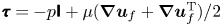 $\boldsymbol{\mathsf{\tau}} =-p\boldsymbol{\mathsf{I}}+\mu (\boldsymbol {\nabla } \boldsymbol{u}_f+\boldsymbol {\nabla } \boldsymbol{u}_f^{\rm T})/2$ is the total fluid stresses,
  $\phi _p$ is the particle volume fraction,
  $\boldsymbol {u}_p$ is the Eulerian particle velocity,
  $\boldsymbol{\mathsf{I}}$ is the identity matrix, T is the transpose operator and
  $({\cdot })_{|p}$ indicates fluid quantities at the particle locations. The first term in (2.3) is the stresses exerted by the undisturbed flow at the particle location. The second term is the stresses caused by the presence of particles which are represented using Stokes drag. When the density ratio is large (
 $\rho _p/\rho _f\gg 1$), as is the case presently, Stokes drag dominates the momentum exchange.
From a scaling analysis of the drag force in (2.3), it is clear that the mass loading  $M=\rho _p\langle \phi _p\rangle /\rho _f$ determines the strength of the coupling. Thus, if the mass loading is vanishingly small, the particle phase has little effect on the stability of the Rankine vortex. Conversely, if the mass loading is large, the interaction between two phases triggers a significant source or sink of energy that may enhance or attenuate perturbations in the flow (Kasbaoui et al. Reference Kasbaoui, Koch, Subramanian and Desjardins2015).
The particle phase is described in the Lagrangian frame. The motion of the  $i$th particle is given by (Maxey & Riley Reference Maxey and Riley1983)
 $$\begin{gather} \frac{{\rm d}\kern0.7pt \boldsymbol{x}_p^i}{{\rm d} t}(t)={\boldsymbol{u}_p^i}(t), \end{gather}$$
 $$\begin{gather}\frac{{\rm d}\boldsymbol{u}_p^i}{{\rm d} t}(t)=\frac{1}{\rho_p}\boldsymbol{\nabla}\boldsymbol{\cdot} \boldsymbol{\mathsf{\tau}} (\boldsymbol{x}_p^i,t)+ \frac{\boldsymbol{u}_f(\boldsymbol{x}_p^i,t)-\boldsymbol{u}^i_p(t)}{\tau_p}, \end{gather}$$
where  $\boldsymbol {x}_p^i$ and
  $\boldsymbol {u}_p^i$ are the position and velocity of the
  $i$th particle, respectively,
  $\tau _p=\rho _pd_p^2/(18\mu )$ is the particle response time and
  $d_p$ the particle diameter. In this study, gravity is ignored in order to focus on inertial effects. Other interactions, including collisions, are negligible due to the large density ratio and low volume fraction. Note that, in the equations above, the instantaneous particle volume fraction and Eulerian particle velocity field are obtained from Lagrangian quantities using
 $$\begin{gather} \phi_p(\boldsymbol{x},t)=\sum_{i=1}^N V_p g (\|\boldsymbol{x}-\boldsymbol{x}_p^i\|), \end{gather}$$
 $$\begin{gather}\phi_p \boldsymbol{u}_p(\boldsymbol{x},t)=\sum_{i=1}^N \boldsymbol{u}_p^i(t) V_p g(\|\boldsymbol{x}-\boldsymbol{x}_p^i\|), \end{gather}$$
where  $V_p={\rm \pi} d_p^3/6$ is the particle volume,
  $g$ represents a Gaussian filter kernel of size
  $\delta _f=3\Delta x$, where
  $\Delta x$ is the grid spacing (Capecelatro & Desjardins Reference Capecelatro and Desjardins2013).
This computational framework was recently applied by the authors in a configuration similar to the one considered here. In Shuai & Kasbaoui (Reference Shuai and Kasbaoui2022), the dynamics of a particle-laden Lamb–Oseen vortex at moderate Stokes numbers is investigated using the Eulerian–Lagrangian methodology presented here. Readers interested in further details about the numerical approach are referred to this study.
2.2. Illustration of the instability
To illustrate the unstable dynamics activated by two-way coupling, we consider a Rankine vortex at the circulation Reynolds number  $Re_\varGamma =\varGamma /(2{\rm \pi} \nu )=1000$, laden with mono-disperse particles having diameter at the Stokes number
  $St_{\varGamma }=\tau _p/\tau _f=0.025$, average volume fraction
  $\langle \phi _p\rangle =1.2\times 10^{-3}$, density ratio
  $\rho _p/\rho _f=830$ and mass loading
  $M=1$. Here,
  $\varGamma$ corresponds to the vortex circulation,
  $r_c$ is the initial vortex core radius,
  $\tau _f= 2{\rm \pi} r_c^2/\varGamma$ is the characteristic fluid velocity,
  $\tau _p=\rho _p d_p^2/(18\mu _f)$ is the particle response time and
  $d_p$ is the particle diameter. The particles are seeded randomly within the core region
  $r\leq r_c$ with velocities matching the fluid velocity at their respective locations. We use the Eulerian–Lagrangian framework described above on uniform Cartesian grid with resolution
  $r_c/\Delta x=50$. The simulations performed here are termed ‘pseudo-two-dimensional’, meaning that the axial direction
  $z$ is resolved with one grid point and taken periodic with a thickness
  $\Delta z=3d_p$. This allows the definition of volumetric quantities such as particle volume and volume fraction. Despite considering pseudo-2-D simulations, a large number of particles must be tracked, here
  $N=376\,612$, due to the large scale ratio
  $r_c/d_p=1400$. The remaining numerical parameters are as in Shuai & Kasbaoui (Reference Shuai and Kasbaoui2022).
In addition to two-way coupled simulations, we perform one-way coupled simulations where the momentum exchange term (2.3) is purposely set to zero. In this way, comparing one-way and two-way simulations reveals the effect of particle feedback on the flow dynamics.
Figure 1 shows the evolution of the isocontours of axial vorticity  $\omega _z$ normalized by the initial centre vorticity
 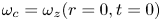 $\omega _c=\omega _z(r=0,t=0)$. Successive snapshots are given between
  $t/\tau _f=0$ and 48. When the particle feedback force is neglected, i.e. in one-way coupling, we observe that the vorticity field remains axisymmetric at all times. Although some viscous diffusion can be observed near the vorticity jump
  $r\sim r_c$, the vorticity magnitude within the core remains mostly flat as viscous effects are too small to cause significant diffusion within the time frame
 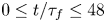 $0\leq t/\tau _f\leq 48$. Contrary to the case of one-way coupling, we observe significant distortion of the flow field when two-way coupling is accounted for. The vorticity field quickly loses its cylindrical symmetry due to the emergence of azimuthal perturbations. The latter grow into vorticity filaments by
  $t/\tau _f\sim 12$ that are gradually convected away from the vortex core. By
  $t/\tau _f\sim 48$, we observe several well-established spiral arms emanating from the vortex core. In this region, vorticity assumes a diffuse profile in contrast to the nearly flat profile seen in one-way coupled simulations.

Figure 1. Isocontours of normalized vorticity ( $\omega _z/\omega _c$) with
  $St_{\varGamma }=0.025$ and
  $Re_{\varGamma }=1000$, for one-way coupling and two-way coupling at five non-dimensional times
  $t/\tau _f$.
Particle dispersion is also significantly impacted by the interaction between the two phases. Figure 2 shows the isocontours of particle volume fraction. When the particle feedback is neglected, the particles gradually accumulate into a ring-shaped cluster of diameter of approximately  $1.5\times r_c$. This clustering dynamics was reported in the earlier work of Druzhinin (Reference Druzhinin1994, Reference Druzhinin1995), Marshall (Reference Marshall2005) and later by Shuai & Kasbaoui (Reference Shuai and Kasbaoui2022). The outward particle ejection is due to preferential concentration (Squires & Eaton Reference Squires and Eaton1991) whereby inertial particles are driven out of strongly vortical regions. Like the carrier flow, the particle distribution is axisymmetric only in one-way coupled simulations. In contrast to these prior observations, two-way coupling leads to a loss of symmetry along with fast and wide dispersion of the particles. The two-way coupled simulations in figure 2 reveal the presence of azimuthal perturbations superimposed on the particle patch at
  $t/\tau _f=12$. The perturbations extend into spiralling particle filaments reminiscent of the density-driven radial Rayleigh–Taylor instability observed by Dixit & Govindarajan (Reference Dixit and Govindarajan2011) and Joly et al. (Reference Joly, Fontane and Chassaing2005). These perturbations destroy the ring structure observed in one-way coupled simulations.
Figure 2. Isocontours of normalized particle volume fraction ( $\phi _p/\langle \phi _p\rangle$) with
  $St_{\varGamma }=0.025$ and
  $Re_{\varGamma }=1000$, for one-way coupling and two-way coupling at five non-dimensional times
  $t/\tau _f$.
The simulations shown in figures 1 and 2 suggest that semi-dilute inertial particles trigger a modal instability. The latter cannot be attributed to purely hydrodynamic nor purely granular effects since the Rankine vortex is neutrally stable and particle–particle interactions are neglected. Rather, it is an instability that arises from the two-way momentum exchange between the two phases.
The instability observed here represents a distinct mechanism from the one studied by Kasbaoui et al. (Reference Kasbaoui, Koch, Subramanian and Desjardins2015). There, the authors show that the interplay between particle settling and preferential concentration activates a non-modal instability in two-way coupled shear flows. This results in the formation of sheets of concentrated particle clusters that rotate to progressively align with the direction of the shear flow. Since particle settling is required for perturbations to grow, the resulting growth rates depend on the gravitational acceleration. In the present work, a modal instability arises regardless of gravitational effects.
3. Linear stability analysis for weakly inertial particles
In this section, we establish a theoretical grounding to this novel two-phase instability through rigorous linear stability analysis (LSA). The analysis is intended to reveal the mechanisms that cause the 2-D particle-laden vortex flow to be unstable, and their functional dependence on the non-dimensional numbers at hand. This study is restricted to the assumption of small, but non-zero, particle inertia such that  $St_{\varGamma }<0.1$.
In the following, we adopt an Eulerian–Eulerian description of the particle-laden flow based on the two-fluid model (Marble Reference Marble1970; Druzhinin Reference Druzhinin1995; Jackson Reference Jackson2000; Kasbaoui et al. Reference Kasbaoui, Koch, Subramanian and Desjardins2015, Reference Kasbaoui, Koch and Desjardins2019b). In this framework, the conservation equations for the fluid phase and particle phase in the two-fluid model read
 $$\begin{gather} \boldsymbol{\nabla}\boldsymbol{\cdot} \boldsymbol{u}_f=0, \end{gather}$$
 $$\begin{gather}\rho_f \left(\frac{\partial \boldsymbol{u}_f}{\partial t}+ \boldsymbol{u}_f\boldsymbol{\cdot}\boldsymbol{\nabla}\boldsymbol{u}_f\right)={-}\boldsymbol{\nabla} p+\mu\nabla^2\boldsymbol{u}_f + \frac{\rho_p V_p n}{\tau_p}(\boldsymbol{u}_p-\boldsymbol{u}_f), \end{gather}$$
 $$\begin{gather}\frac{\partial \rho_p n}{\partial t} +\boldsymbol{\nabla}\boldsymbol{\cdot} (\rho_p n\boldsymbol{u}_p)= 0, \end{gather}$$
 $$\begin{gather}\frac{\partial \rho_p n \boldsymbol{u}_p}{\partial t} +\boldsymbol{\nabla}\boldsymbol{\cdot} (\rho_p n \boldsymbol{u}_p \boldsymbol{u}_p) ={-} \frac{\rho_p V_p n}{\tau_p}(\boldsymbol{u}_p-\boldsymbol{u}_f), \end{gather}$$
where  $\boldsymbol {u}_f$ is the fluid velocity,
  $\boldsymbol {u}_p$ is the particle velocity,
  $V_p$ is the particle volume and
  $n=\phi _p/V_p$ is the particle number density. Equations (3.1) and (3.2) express mass and momentum conservation for the fluid phase, respectively. Equations (3.3) and (3.4) express mass and momentum conservation for the particle phase. In these equations, it is assumed that the particles experience a hydrodynamic force equal to Stokes drag. The two phases are coupled through Stokes drag, as seen in (3.2) and (3.4). If the particle feedback force is dropped from the fluid momentum equation (3.2), the evolution of the fluid becomes decoupled from that of the particles. The fluid evolves as in single phase, and the flow may not become unstable, as shown in § 2 and Michalke & Timme (Reference Michalke and Timme1967). The momentum exchange between the two phases is critical for the development of an instability.
Compared with the Eulerian–Lagrangian framework presented in § 2, the form of the differential equations in the two-fluid model is more suitable for theoretical analysis using LSA. Still, the two approaches yield qualitatively and quantitatively similar evolution of particle-laden flows in the semi-dilute regime provided that particle inertia is small. Further details on the comparison of the two formulations can be found in Kasbaoui et al. (Reference Kasbaoui, Koch and Desjardins2019a). Thus, we restrict the analysis to cases where  $St_{\varGamma } \ll 1$.
Under the assumption of weakly inertial particles, it is possible to further simplify the governing equations by adopting the fast equilibrium approximation (see the work by Balachandar and coworkers (Ferry & Balachandar Reference Ferry and Balachandar2001, Reference Ferry and Balachandar2002; Rani & Balachandar Reference Rani and Balachandar2003) and Maxey Maxey Reference Maxey1987). Provided that particle inertia is low enough, it is possible to express the particle velocity field as
 \begin{equation} \boldsymbol{u}_p=\boldsymbol{u}_f - \tau_p\left(\frac{\partial \boldsymbol{u}_f}{\partial t}+ \boldsymbol{u}_f\boldsymbol{\cdot}\boldsymbol{\nabla}\boldsymbol{u}_f\right)+O(\tau_p^2), \end{equation}
where it is seen that the particles deviate from the fluid streamlines by a small inertial correction. Owing to the preferential concentration mechanism, particles suspended in a vortex do not follow the closed-loop streamlines of the carrier flow. Instead, they tend to migrate outward radially at a rate controlled by their Stokes number.
Next, we combine (3.5) with the conservation equations (3.1), (3.2) and (3.3). Using  $r_c$,
  $\varGamma /(2{\rm \pi} r_c)$ and the core number density
  $n_0$ as the reference length scale, velocity scale and number density, respectively, the following non-dimensionalized equations are obtained:
 $$\begin{gather} \boldsymbol{\nabla}\boldsymbol{\cdot} \boldsymbol{u}^*=0, \end{gather}$$
 $$\begin{gather}(1+M n^*)\left(\frac{\partial \boldsymbol{u}^*}{\partial t^*}+\boldsymbol{u}^*\boldsymbol{\cdot} \boldsymbol{\nabla}\boldsymbol{u}^*\right)={-}\boldsymbol{\nabla} p^* + \frac{1}{Re_{\varGamma}} \nabla^2\boldsymbol{u}^*, \end{gather}$$
 $$\begin{gather}\frac{\partial n^*}{\partial t^*} +\left(\boldsymbol{u}^*-St_{\varGamma} \left(\frac{\partial \boldsymbol{u}^*}{\partial t^*}+\boldsymbol{u}^*\boldsymbol{\cdot}\boldsymbol{\nabla}\boldsymbol{u}^*\right)\right) \boldsymbol{\cdot}\boldsymbol{\nabla} n^*=St_{\varGamma} n^*\boldsymbol{\nabla}\boldsymbol{u}^*:\boldsymbol{\nabla}\boldsymbol{u}^*, \end{gather}$$
where the stared variables denote non-dimensional quantities,  $Re_{\varGamma }=\varGamma /(2{\rm \pi} \nu )$ is the circulation Reynolds number,
  $St_{\varGamma }=\tau _p r_c^2/\varGamma$ is the circulation Stokes number and
  $M=\rho _p V_p n_0/\rho _f$ is the mass loading. Equation (3.7) is derived by injecting the small Stokes expansion (3.5) into the momentum exchange term in (3.2). Likewise, (3.8) is obtained from (3.3) by replacing the particle velocity field with the expansion (3.5). For ease of notation, we drop the stars in the rest of the analysis.
In this form, the particle phase is coupled with the fluid through the preferential concentration term appearing on the right-hand side of (3.8). Since Squires & Eaton (Reference Squires and Eaton1991), the preferential concentration term has been widely studied (Batchelor & Nitsche Reference Batchelor and Nitsche1991; Squires & Eaton Reference Squires and Eaton1991; Wang & Maxey Reference Wang and Maxey1993; Druzhinin Reference Druzhinin1995). It is understood that this term relates to compressibility effects of the particle phase since  $\boldsymbol {\nabla }\boldsymbol {\cdot } \boldsymbol {u}_p\simeq -\tau _p\boldsymbol {\nabla } \boldsymbol {u}_f:\boldsymbol {\nabla } \boldsymbol {u}_f$ for low inertia particles. This term may be further expressed as
  $\boldsymbol {\nabla }\boldsymbol {u}_f:\boldsymbol {\nabla } \boldsymbol {u}_f=S^2-R^2$, where
  $S^2$ and
  $R^2$ represent the second invariants of the fluid strain rate tensor
  $S=(\boldsymbol {\nabla } \boldsymbol {u} +\boldsymbol {\nabla } \boldsymbol {u}^{\rm T})/2$ and rotation tensor
  $R=(\boldsymbol {\nabla } \boldsymbol {u} -\boldsymbol {\nabla } \boldsymbol {u}^{\rm T})/2$ (Squires & Eaton Reference Squires and Eaton1991). When the local strain exceeds the local rotation, this term is positive leading to particle accumulation. Conversely, when this term is negative, the particles are expelled. As a result, inertial particles are progressively depleted from rotational regions, such as vortex cores. The formation of a ring cluster shown in figure 2 is a direct effect of preferential concentration.
The number density term in (3.7) suggests that the particles may lead to a non-Boussinesq dynamics similar to that observed in stratified fluids. In particular, Dixit & Govindarajan (Reference Dixit and Govindarajan2010) showed that density gradients could lead to destabilization of a 2-D vortex. Sipp et al. (Reference Sipp, Fabre, Michelin and Jacquin2005) showed that density gradients produce two distinct kinds of instability, namely the centrifugal instability, which mainly affects axisymmetric eigenmodes, and the Rayleigh–Taylor instability, which mainly affects non-axisymmetric eigenmodes. If particle inertia is negligible, one may ignore the preferential concentration term, and treat the suspension as a fluid with effective density  $\rho _{{eff}}=\rho _f+\rho _p V_p n$. In such a case, the suspension would be susceptible to the instabilities of variable density vortex flows previously mentioned. These effects are revisited for the case of non-inertial particles in § 3.3, and then extended to the case of weakly inertial particles in § 3.4.
3.1. Base state
In the remainder of the manuscript, we perform a LSA for a base state initially comprising monodisperse particles seeded randomly within a disk of non-dimensional size  $r_p$ and a Rankine vortex. A schematic of the configuration is given in figure 3(a). The non-dimensional base fluid azimuthal velocity field
  $u^b_{f,\theta }$ and number density fields
  $n^b$ are given by
 $$\begin{gather} u^b_{f,\theta}(r,t=0)= \left\{\begin{array}{@{}ll} r, & r\leq1\\ 1/r, & r>1 \end{array}\right. \end{gather}$$
 $$\begin{gather}n^b(r,t=0)= \left\{\begin{array}{@{}ll} 1, & \mbox{if } r\leq r_p\\ 0, & \mbox{otherwise.} \end{array}\right. \end{gather}$$
Figure 3. Configuration studied using LSA: (a) a Rankine vortex with core radius  $r_c$ is seeded with particles within the region
  $r\leq r_p$; (b) the resulting preferential concentration term is negative within the vortex core, which causes inertial particles in this region to be ejected outward.
Note that the task of defining a base state requires careful consideration when the suspended particles are inertial. Even when the base flow is steady, the particle distribution may be unsteady due to the outward ejection of particles caused by the preferential concentration term in (3.8). The latter is plotted in figure 3(b) for the Rankine vortex in (3.9). The preferential concentration term is negative within the core ( $r<1$), showing that it acts as a sink in this region. Conversely, the preferential concentration term is positive away from the core (
 $r>1$), corresponding to regions where the particles will accumulate. Thus, the base number density
  $n^b$ in (3.10) is expected to vary as time progresses.
The time evolution of the base state may be obtained by solving (3.6), (3.7) and (3.8). Considering an inviscid and axisymmetric state ( $\partial ()/\partial \theta = 0$), the equations dictating the evolution of the base state are
 $$\begin{gather} \frac{\partial u_{\theta}^b}{\partial t} = 0, \end{gather}$$
 $$\begin{gather}\frac{\partial n^b}{\partial t} + \frac{St_{\varGamma}}{r} \frac{\partial}{\partial r} ((u_{\theta}^{b})^2 n^b) = 0. \end{gather}$$
Following Druzhinin (Reference Druzhinin1994), it is possible to obtain an analytical solution for the unsteady number density by applying the method of characteristics. Denoting the initial particle number density in (3.10) by  $n_0^b = n^b(r,0)$, the unsteady number density is written as
 \begin{equation} n^b(r,t)=
\left\{\begin{array}{@{}ll} \exp({-2 St_{\varGamma}\, t})
n_0^b\left(r \exp({- St_{\varGamma}\, t})\right), &
\mbox{if } r\leq 1\\ \dfrac{r^2}{\sqrt{r^4 - 4
St_{\varGamma}\, t}} n_0^b\left((r^4 - 4 St_{\varGamma}\,
t)^{1/4} \right), & \mbox{if } r>1 \ \mbox{and}\ t\leq
t_{{cr}}\\ \left(rr_0\right)^2 n_0^b\left( r_0\right), &
\mbox{if } r>1 \ \mbox{and}\ t> t_{{cr}} \end{array}\right.
\end{equation}
\begin{equation} n^b(r,t)=
\left\{\begin{array}{@{}ll} \exp({-2 St_{\varGamma}\, t})
n_0^b\left(r \exp({- St_{\varGamma}\, t})\right), &
\mbox{if } r\leq 1\\ \dfrac{r^2}{\sqrt{r^4 - 4
St_{\varGamma}\, t}} n_0^b\left((r^4 - 4 St_{\varGamma}\,
t)^{1/4} \right), & \mbox{if } r>1 \ \mbox{and}\ t\leq
t_{{cr}}\\ \left(rr_0\right)^2 n_0^b\left( r_0\right), &
\mbox{if } r>1 \ \mbox{and}\ t> t_{{cr}} \end{array}\right.
\end{equation}
where  $t_{{cr}}=(r^4-1)/4St_{\varGamma }$ and
  $r_0(r,t)$ is obtained from the equation
  $4\log r_0+r_0^4=r^4-4St_{\varGamma } t$. Despite the explicit time dependence of the base number density field
  $n^b$, a quasi-steady assumption may be employed for weakly inertial particles. Under this assumption, the base state is assumed frozen at
  $t=0$. This assumption is justified provided that perturbations grow on a time scale that is much faster than the characteristic evolution time of the number density field. From solution (3.13), it can be seen that the time scale for the development of number density inhomogeneity is
  $\tau _c=\tau _f/St_{\varGamma }$. Shuai & Kasbaoui (Reference Shuai and Kasbaoui2022) showed from Eulerian–Lagrangian simulations that the time required to eject most particles from the core of a vortex is
  ${\sim }3\tau _c$. This time scale may be significantly larger than the flow inertial time scale
  $\tau _f$ when
  $St_{\varGamma }\ll 1$. For such weakly inertial particles with low inertia, particle clustering is slow compared with inertial effects of the carrier vortex flow. Since we expect the instability to develop on a time scale comparable to the flow inertial time scale, the assumption of quasi-steady number density is justified.
3.2. Linearized equations
We assume that the base state discussed previously is subject to small perturbations  $n'$ and
  $\boldsymbol {u}'$ such that the total number density and fluid velocity are
  $n=n^b+n'$ and
  $\boldsymbol {u}=\boldsymbol {u}^b+\boldsymbol {u}'$. Taking the inviscid limit (
 $Re_{\varGamma } \rightarrow \infty$) and linearizing (3.6) and (3.7), the fluid perturbation is subject to the following equations:
 $$\begin{gather} \frac{1}{r}\frac{\partial (r u_{r}')}{\partial r} + \frac{1}{r}\frac{\partial u_{\theta}'}{\partial \theta}=0, \end{gather}$$
 $$\begin{gather}(1+Mn^b)\left( \frac{\partial u_{r}'}{\partial t} +\frac{u^b_{\theta}}{r}\frac{\partial u_{r}'}{\partial \theta} - 2 \frac{u^b_{\theta}u'_{\theta}}{r} \right) - M n' \frac{(u^b_{\theta})^2}{r} ={-}\frac{\partial p'}{\partial r}, \end{gather}$$
 $$\begin{gather}(1+Mn^b)\left( \frac{\partial u_{\theta}'}{\partial t} +\frac{ u^b_{\theta}}{r} \frac{\partial u_{\theta}'}{\partial \theta} - u'_{r}\frac{\partial u^b_{\theta}}{\partial r}+ \frac{u'_{r}u^b_{\theta}}{r}\right) ={-}\frac{1}{r}\frac{\partial p'}{\partial \theta}, \end{gather}$$
where (3.14) represents mass conservation in cylindrical coordinates, and (3.15) and (3.16) represent the radial and azimuthal fluid momentum conservation, respectively. Introducing the base state angular velocity  $\varOmega ^b=u^b_{\theta }/r$ and axial vorticity
  $\omega ^b_z=(\partial (r u^b_{\theta })/\partial r)/r$, (3.15) and (3.16) become
 $$\begin{gather} (1+Mn^b)\left( \left(\frac{\partial}{\partial t} + \varOmega^b \frac{\partial}{\partial \theta}\right)u'_{r} - 2\varOmega^b u'_{\theta}\right)- M n' r(\varOmega^b)^2 ={-}\frac{\partial p'}{\partial r}, \end{gather}$$
 $$\begin{gather}(1+Mn^b)\left( \left(\frac{\partial}{\partial t} + \varOmega^b \frac{\partial}{\partial \theta}\right)u'_{\theta} +\omega_z^b u'_{r}\right) ={-}\frac{1}{r}\frac{\partial p'}{\partial \theta}. \end{gather}$$
The evolution of the perturbation axial vorticity, i.e.
 \begin{equation} \omega'_z=\frac{1}{r}\frac{\partial}{\partial r}(ru'_{\theta})- \frac{1}{r}\frac{\partial u'_{r}}{\partial \theta}, \end{equation}
is obtained by combing (3.17) and (3.18)
 \begin{align} & \left(\frac{\partial}{\partial t} + \varOmega^b \frac{\partial}{\partial \theta}\right)\omega'_z + \frac{\partial \omega^b_z}{\partial r} u'_{r} \nonumber\\ &\quad ={-}\frac{M}{1+Mn^b} \left( (\varOmega^b)^2\frac{\partial n'}{\partial \theta}+ \frac{\partial n^b}{\partial r} \left(\left(\frac{\partial}{\partial t} + \varOmega^b \frac{\partial}{\partial \theta}\right)u'_{\theta} + \omega^b_z u'_{r}\right)\right). \end{align}
The number density perturbation is solution to the following equation:
 \begin{align} & \frac{\partial n'}{\partial t}+\varOmega^b \frac{\partial n' }{\partial \theta}+ \frac{\partial n^b}{\partial r} u'_{r} \nonumber\\ &\quad =St_{\varGamma}\left( \frac{\partial n_b}{\partial r} \left(\frac{\partial u'_{r}}{\partial t}+\varOmega^b \frac{\partial u'_{r}}{\partial \theta} \right) -r(\varOmega^b)^2 \frac{\partial n'}{\partial r}-2\varOmega^b\frac{\partial n^b}{\partial r} u'_{\theta}\right) \nonumber\\ &\qquad +St_{\varGamma} n^b\frac{2}{r}\left(\frac{\partial (r\varOmega)}{\partial r} \left(\frac{\partial u'_{r}}{\partial \theta}-u'_{\theta} \right)-r\varOmega^b \frac{\partial u'_{\theta}}{\partial r}-St_{\varGamma}\frac{1}{r}\frac{\partial }{\partial r}((r\varOmega^b)^2)n' \right). \end{align}
 Next, the perturbations  $n'$,
$n'$,  $u_{\theta }'$ and
  $u_{r}'$ are decomposed using Fourier series as
 \begin{equation} [u_{r}'(r,\theta,t),u_{\theta}'(r,\theta,t),n'(r,\theta,t)] = [\hat{u}_r(r,t),\hat{u}_{\theta}(r,t),\hat{n}(r,t)] {\rm e}^{{\rm i} m \theta}, \end{equation}
where  $m$ represents the mode number. Combining this form of perturbations with (3.20) and (3.21), the set of linear equations becomes
 \begin{align} & \mathcal{D} \left(\bar{n} r \mathcal{D} \left(r \frac{\partial \hat{u}_r}{\partial t}\right) \right) - \bar{n} m^2 \frac{\partial \hat{u}_r}{\partial t} + {\rm i} m \varOmega^b ( \mathcal{D} (\bar{n} r \mathcal{D} (r \hat{u}_r) ) - \bar{n} m^2 \hat{u}_r ) \nonumber\\ &\quad - {\rm i} m r \mathcal{D}(\bar{n} \omega_z^b) \hat{u}_r + r m^2 (\varOmega^b)^2 M \hat{n} = 0, \end{align}
 \begin{align} & \left(\frac{\partial n}{\partial t} - St_{\varGamma} \mathcal{D}(n^{b}) \frac{\partial \hat{u}_r}{\partial t} \right) + {\rm i} m \varOmega^b (n - St_{\varGamma} \mathcal{D}(n^{b}) \hat{u}_r ) + \mathcal{D}(n^{b}) \hat{u}_r \nonumber\\ &\quad - {\rm i}St_{\varGamma} \left\lbrace \frac{{\rm i}}{r} \mathcal{D} (r^2 (\varOmega^b)^2 \hat{n}) - \frac{2}{m} \varOmega^b \mathcal{D}(n^{b}) \mathcal{D} (r \hat{u}_r)\right. \nonumber\\ &\quad \left. - \frac{2 n^b}{m r} [ \mathcal{D} ( \varOmega^b r \mathcal{D} (r \hat{u}_r) ) - m^2 \mathcal{D}(r \varOmega^b) \hat{u}_r] \right\rbrace = 0. \end{align}
Here,  $\mathcal {D}$ denotes the derivative with respect to
  $r$ and
  $\bar {n}=1+Mn^b$. Note that (3.23) and (3.24) retain the two-way coupling required for an instability.
Using the assumption of quasi-steady base state discussed above, we perform a modal stability analysis with the base state being frozen in time by considering perturbations that have an exponential dependence on time. Under this consideration, the perturbations can be written as
 \begin{equation} \left[\hat{u}_r(r,t),\hat{u}_{\theta}(r,t),\hat{n}(r,t)\right] = \left[u_r(r),u_{\theta}(r),n(r)\right] {\rm e}^{\sigma t}, \end{equation}
where  $\sigma$ is the complex growth rate. Perturbations whose real part of
  $\sigma$, is positive grow without bound. Thus, the condition for an unstable base state is
  ${\rm Re}(\sigma ) >0$. Injecting the forms (3.25) into (3.23) and (3.24), we obtain
 \begin{equation} (\sigma + {\rm i} m \varOmega^b) [ \mathcal{D} \left(\bar{n} r \mathcal{D} (r u_r)\right) - \bar{n} m^2 u_r ] - {\rm i} m r \mathcal{D}(\bar{n} \omega_z^b) u_r + r m^2 (\varOmega^b)^2 M n = 0, \end{equation}
 \begin{align} & (\sigma + {\rm i} m
\varOmega^b) (n - St_{\varGamma} \mathcal{D}(n^{b})
u_r ) + \mathcal{D}(n^{b}) u_r + St_{\varGamma}
\left\lbrace \frac{1}{r} \mathcal{D} (r^2 (\varOmega^b)^2
n) + \frac{2 {\rm i}}{m} \varOmega^b \mathcal{D}(n^{b})
\mathcal{D} (r u_r)\right. \nonumber\\ &\quad \left. {} +
\frac{2 {\rm i} n^b}{m r} [ \mathcal{D} (
\varOmega^b r \mathcal{D} (r u_r) ) - m^2
\mathcal{D}(r \varOmega^b) u_r ] \right\rbrace = 0.
\end{align}
\begin{align} & (\sigma + {\rm i} m
\varOmega^b) (n - St_{\varGamma} \mathcal{D}(n^{b})
u_r ) + \mathcal{D}(n^{b}) u_r + St_{\varGamma}
\left\lbrace \frac{1}{r} \mathcal{D} (r^2 (\varOmega^b)^2
n) + \frac{2 {\rm i}}{m} \varOmega^b \mathcal{D}(n^{b})
\mathcal{D} (r u_r)\right. \nonumber\\ &\quad \left. {} +
\frac{2 {\rm i} n^b}{m r} [ \mathcal{D} (
\varOmega^b r \mathcal{D} (r u_r) ) - m^2
\mathcal{D}(r \varOmega^b) u_r ] \right\rbrace = 0.
\end{align}
The above pair of equations can be treated as an eigenvalue problem to obtain the stability parameters.
3.3. Limit of inertia-less particles  $(St_{\varGamma }=0)$ and non-Boussinesq effects

As previously discussed, with the absence of particle inertia ( $St_{\varGamma }=0$), the preferential concentration term drops out of the governing equations. Also, the base state in the case of
  $St_{\varGamma }=0$ remains constant over time, as shown in (3.11) and (3.12). Simplified linear equations can be obtained as
 $$\begin{gather} (\sigma + {\rm i} m \varOmega^b) [ \mathcal{D} \left( \bar{n} r \mathcal{D} (r u_r) \right) - \bar{n} m^2 u_r ] - {\rm i} m r \mathcal{D}(\bar{n} \omega_z^b) u_r + r m^2 (\varOmega^b)^2 M n = 0, \end{gather}$$
 $$\begin{gather}n ={-} \frac{\mathcal{D}(n^b) }{(\sigma + {\rm i} m \varOmega^b)} u_{r}. \end{gather}$$
The above linearized equations are identical to the equations for a vortex with a radially stratified density written by Dixit & Govindarajan (Reference Dixit and Govindarajan2011). Without the particle inertia, the problem reduces to that of a vortex with a density stratification induced by particles. Following the approach of Dixit & Govindarajan (Reference Dixit and Govindarajan2011), it is possible solve (3.28) and (3.29) analytically and obtain a dispersion relation for a Rankine vortex. This is done by computing the perturbation velocity and number density fields separately in regions of  $r<1$,
  $1< r< r_p$ and
  $r>r_p$. The constants subsequently obtained are found using the continuity condition at the jump locations
  $r=1$ and
  $r = r_p$. The dispersion relation, thus obtained, is written as
 \begin{equation} \sigma^3 + a_2 \sigma^2 + a_1 \sigma + a_0 = 0, \end{equation}
where
 $$\begin{gather} a_2 = {\rm i}( m + 2 m r_p^{{-}2} - 1 - At \, r_p^{{-}2m} ), \end{gather}$$
 $$\begin{gather}a_1 = m r_p^{{-}2} [ 2 - m ( 2 + r_p^{{-}2} ) - At ( r_p^{{-}2} - 2 r_p^{{-}2m})], \end{gather}$$
 $$\begin{gather}a_0 = {\rm i} m (1-m) r_p^{{-}4} [m + At (1 - r_p^{{-}2m} )], \end{gather}$$
where  $At=M/(2+M)$ is the Atwood number. The latter is a non-dimensional number that commonly arises in density stratified flows. Here, considering the particle–fluid mixture as a fluid with effective density
  $\rho _{eff}=1+(\rho _p/\rho _f) V_p n=1+M n$, we see that in the core
  $\rho _{eff} (r)= 1+M=\rho _{max}$ for
  $r\leq 1$, while
  $\rho _{eff}=1=\rho _{min}$ away from the core (
 $r\geq 1$). Thus, the Atwood number is
  $At=(\rho _{max}-\rho _{min})/(\rho _{max}+\rho _{min})$, which measures the relative magnitude of the density jump between the inner and outer regions.
Figures 4(a) and 4(b) show contours of growth rates for wavenumbers  $m = 2$ and
  $4$, respectively, in the
  $At$–
$At$– $r_p$ plane. The white space labelled ‘S’ represents the region of stability. Thus there exists a critical radius,
  $r_p^{{cr}}$, such that instability would only be observed when the density jump is located beyond
  $r_p^{{cr}}$. Using the property of the cubic equation (3.30) one can obtain a relation for
  $r_p^{{cr}}$ as a function of
  $m$ and
  $At$, which, on further expanding for
  $At\ll 1$, yields
 \begin{equation} r_p^{{cr}} = r^{{Kelvin}}\left[1-\frac{3}{2}\left\{\frac{At}{4m^2} \left(\frac{m-1}{m}\right)^{m-1}\right\}^{1/3}\right]+{O}(At^{2/3}), \end{equation}
where  $r^{{Kelvin}}=\sqrt {m/(m-1)}$ is the critical radius corresponding to the discrete Kelvin mode (Roy & Subramanian Reference Roy and Subramanian2014). As is evident from the complete numerical solution and the above small-
 $At$ asymptotic expression, the region of stability shrinks as the wavenumber increases, suggesting that higher modes are more unstable. In addition, higher values of growth rates are achieved with increasing values of Atwood number and with the value of
  $r_p$ closer to one. This suggests that the configuration at
  $r_p=1$ with infinitely heavy core (
 $M\rightarrow \infty$) is the most unstable configuration.

Figure 4. Contours of the analytically obtained growth rate (3.30) in the  $At-r_p$ plane for a Rankine vortex with
  $St_{\varGamma } = 0$: (a)
  $m = 2$; (b)
  $m = 4$.
To further study the influence of the Atwood number on the critical wavenumber, we investigate the specific case of  $r_p = 1$, for which the dispersion relation reduces to
 \begin{equation} \sigma = \frac{{\rm i}}{2}(1 + At) - {\rm i} m \pm \frac{{\rm i}}{2}\sqrt{(1 + At)^2 - 4 m At}. \end{equation}
For  $r_p = 1$, the third root of (3.30) corresponds to a mode rotating with core angular frequency (
 $\sigma =-{\rm i}m$.) The expression (3.35) indicates the critical wavenumber (
 $m_{cr}$) for unstable system is
 \begin{equation} m_{cr} = \frac{(1 + At)^2}{4 At} = \frac{(1+M)^2}{(2+M)M}. \end{equation}
The above expression shows that increasing the Atwood number, or equivalently the mass loading, promotes the instability by making lower-wavenumber modes unstable. In the limit case where  $M\rightarrow \infty$, corresponding to
  $At\rightarrow 1$, the critical wavenumber becomes
  $m_{cr}\rightarrow 1$, showing that all modes are unstable. Conversely, when
  $M\rightarrow 0$, none of the modes are unstable since
  $m_{cr}\rightarrow \infty$. Thus, we recover the known behaviour for an unladen Rankine vortex (
 $M\rightarrow 0$).
From expression (3.35), the growth rate of unstable modes ( $m\geq m_{cr}$) is given by
 \begin{equation} {\rm Re}(\sigma)=\tfrac{1}{2}\sqrt{4m At-(1+At)^2}\simeq \sqrt{m At} \quad \text{for } m\gg 1. \end{equation}
From this relationship, we draw two conclusions. First, a naturally developing instability, i.e. unforced, will tend to emerge at high wavenumbers since  ${\rm Re}(\sigma )$ increases with
  $m$. Viscous effects are expected to curb
  ${\rm Re}(\sigma )$ beyond a certain mode number
  $m$. Because viscous effects are not accounted for in the present formulation, it is not possible to estimate a priori which mode would emerge naturally. The second conclusion is that the growth rate increases with mass loading. The maximum growth rate obtained when
  $M\rightarrow \infty$ (
 $At\rightarrow 1$) is
  ${\rm Re}(\sigma )_{max}=\sqrt {m}$.
3.4. Effects of particle inertia
Next, we consider the effects of non-zero particle inertia ( $St_{\varGamma } \neq 0$) on the stability of the particle-laden Rankine vortex. For this, we first perform a modal stability analysis by solving (3.26) and (3.27) with a frozen base state.
For the case where the Rankine vortex and particle core have equal radii, i.e.  $r_p=1$, a dispersion relation can be obtained analytically
 \begin{equation} \sigma^2 - {\rm i}\left( 1 + At - 2 m + {\rm i} m At St_{\varGamma} \right) \sigma - m (m - 1 - {\rm i} (m-2) At St_{\varGamma}) = 0, \end{equation}
which yields
 \begin{align} \sigma = \frac{{\rm i}}{2} (1+At + {\rm i} At St_{\varGamma} m) - {\rm i} m \pm \frac{{\rm i}}{2}\sqrt{(1+At + {\rm i} At St_{\varGamma} m)^2 -4 m (At+2{\rm i}AtSt_{\varGamma})} .\end{align}
Note that expression (3.39) collapses on (3.35) when  $St_{\varGamma }\rightarrow 0$. The corresponding expressions for the eigenfunctions of a mode
  $m$ are
 $$\begin{gather} u_r = \left\{\begin{array}{@{}ll} r^{(m-1)}, & \mbox{if }r \leq 1\\ r^{-(m+1)}, & \mbox{otherwise} \end{array}\right. \end{gather}$$
 $$\begin{gather}n = \left( - St_{\varGamma} + \frac{1 + 2 {\rm i}St_{\varGamma}}{\sigma + {\rm i} m} \right) \delta (r-1). \end{gather}$$
Here,  $\delta (r-1)$ denotes the Dirac delta function. These functions correspond to perturbations that are concentrated at the number density and vorticity jumps
  $r=r_p=1$. To further study the stabilizing/destabilizing effect of particle inertia, we expand the expression for growth rate (3.39) in a series of
  $St_{\varGamma }$ as
 \begin{align} \sigma = \sigma\vert_{St_{\varGamma}=0} -\frac{m St_{\varGamma} At}{2}\pm \left\{\frac{m At(3-At)}{2\sqrt{\varDelta}}St_{\varGamma}+ \frac{{\rm i} m^2 At^2 ((m-2)At+2)}{\varDelta^{3/2}}St_{\varGamma}^2\right\}+{O}(St_{\varGamma}^3), \end{align}
where  $\varDelta =(1 + At)^2 - 4 m At$. For
  $St_{\varGamma }=0$,
  $\varDelta <0$ provides the condition for instability for a fixed
  $m$, that is, a mode
  $m$ is stable if
  $At< At_{{cr}}=2m-1-2\sqrt {m(m-1)}$. For
  $St_{\varGamma }\neq 0$, particle inertia can play contrasting roles. For
  $At< At_{{cr}}$, the dispersed phase destabilizes the vortex
 \begin{equation} {\rm Re}(\sigma)=\frac{mAtSt_{\varGamma}}{2}\left\{\frac{3-At}{\sqrt{\varDelta}}-1\right\}+{O}(St_{\varGamma}^3), \end{equation}
while for  $At>At_{\textrm {cr}}$, the dispersed phase stabilizes the vortex
 \begin{equation} {\rm Re}(\sigma)=\frac{1}{2}\sqrt{|\varDelta|} - \frac{m St_{\varGamma} At}{2}+{O}(St_{\varGamma}^2).\end{equation}
Figure 5(a) shows the variation of growth rate plotted over a range of Stokes numbers for wavenumber  $m = 2$. With the smaller value of Atwood number
  $At = 0.1$, the growth rates decrease with increasing Stokes numbers. However, the trends get reversed for higher Atwood numbers, with the growth rates increasing with increasing Stokes numbers, confirming the predictions from the asymptotic calculations (3.43) and (3.44). Figure 5(b) plots the growth rates over a range of Atwood numbers for three values of Stokes numbers. It is found that the growth rate is always positive as long as the Atwood number
  $At$ and Stokes number
  $St_{\varGamma }$ are non-zero. This indicates that destabilization of the vortex by the particles is guaranteed as long as the particle inertia is non-zero.

Figure 5. Growth rates  ${\rm Re}(\sigma )$ for a Rankine vortex with
  $r_p = 1$ and
  $m = 2$ obtained analytically (3.38), (a)
  ${\rm Re}(\sigma ) - {\rm Re}(\sigma )|_{St_{\varGamma } = 0}$ plotted over a range of Stokes numbers for
  $At = 0.1$ (—),
  $At = 0.3$ (- - -),
  $At = 0.9$ (
 $\cdots$); (b)
  ${\rm Re}(\sigma )$ plotted over a range of Atwood numbers for
  $St_{\varGamma } = 0$ (red),
  $St_{\varGamma } = 0.01$ (black) and
  $St_{\varGamma } = 0.1$ (blue).
For cases where  $r_p> 1$, we solve (3.26) and (3.27) numerically using the Chebyshev spectral collocation method (Trefethen Reference Trefethen2000). To handle the discontinuities, we smooth the base state using hyperbolic tangents of thickness
  $\varDelta =0.01$. Figures 6(a) and 6(b) show the contours of growth rate in the
  $At - r_p$ plane for Stokes numbers
  $0.01$ and
  $0.1$, respectively. Unlike the case of
  $St_{\varGamma } = 0$ (see figure 4), there is no region of stability, indicating that mode
  $m=2$ is always unstable when the particles are inertial. Further, the particle-laden vortex is unstable even for values of
  $r_p$ larger than 1. Whereas the results for non-inertial particles are similar to those obtained by Dixit & Govindarajan (Reference Dixit and Govindarajan2011), inclusion of particle inertia breaks the equivalence with a radially stratified Rankine vortex. For the case
  $St_{\varGamma }=0.01$, the optimal value of
  $r_p$ leading to the largest growth rate is slightly in excess of 1 for low values of
  $At$, and approaches
  $r_p=1$ as
  $At$ increases. For the larger inertia case
  $St_{\varGamma }=0.1$,
  $r_p=1$ leads to the largest growth rates for all values of
  $At$.
$At$.

Figure 6. Growth rates  ${\rm Re}(\sigma )$ of mode
  $m=2$ in the
  $At$–
$At$– $r_p$ plane obtained numerically using a smoothed Rankine profile: (a)
  $St_{\varGamma } = 0.01$; (b)
  $St_{\varGamma } = 0.1$.
4. Comparison of LSA with Euler–Lagrange simulations
In order to validate the LSA, we compare the analytical results with those from Eulerian–Lagrangian simulations of the two-way coupled system. To make the comparison tractable and accessible, the case  $r_p=1$ is used as the benchmark since the growth rates can be computed analytically from (3.38).
Table 1 lists a summary of non-dimensional parameters for 8 cases presently considered. In all these simulations, the Stokes number, circulation Reynolds number  $Re_{\varGamma }$ and ratio
  $r_p/r_c$ are fixed at
  $0.002$,
  $5000$ and
  $1$, respectively. The Stokes number is sufficiently small such that the initial state can be considered quasi-steady and comparisons with LSA are permissible. In dimensional terms, the carrier fluid has density
  $\rho _f=1.2\,{\rm kg}\,{\rm m}^{-3}$ and viscosity
  $\mu _f = 1.8 \times 10^{-5}\,{\rm kg}\,{\rm m}^{-1}\, s^{-1}$. The initial vortex core is
  $r_c=0.385\,\mathrm {m}$ and circulation is
  $\varGamma =9.42 \times 10^{-2}\,{\rm m}^{2}\,{\rm s}^{-1}$. Particles are seeded with density
  $\rho _p = 1000\,{\rm kg}\,{\rm m}^{-3}$ and average volume fraction
  $\langle \phi _p\rangle =1.2\times 10^{-3}$. In all cases chosen, the ratio
  $r_c/d_p$ is large (of the order
  $10^4$), such that fluctuations due to the discrete particle forcing fall well below the viscous dissipation scale. In this way, the coupling between the fluid and particles occurs primarily through a collective particle dynamics at scales comparable to
  $r_c$, rather than discrete effects at scales comparable to the inter-particle distance.
Table 1. Non-dimensional parameters considered in simulations.

The initial conditions of the numerical simulations correspond to a superposition of the base Rankine vortex and the perturbation eigenmodes (3.40) and (3.41). In order to capture the linear regime described by the LSA, the perturbations are initialized with a small amplitude  $\epsilon =0.03$. The Dirac delta function that appears in the eigenfunctions (3.40) and (3.41) is discretized on the Cartesian grid according to the radial distance
  $l_i$ (
 $i=1,2,3,4$) between the vortex core and the four vertices of each cell. Cells that are intersected by the discontinuity (
 $\max (l_i)>1$ and
  $\min (l_i)<1$) have
  $\delta (r-1)=1/(\Delta x\Delta y)$, whereas
  $\delta (r-1)=0$ everywhere else. The Lagrangian particles are generated randomly within each cell based on the number density computed with the aforementioned discrete perturbation. The particle velocities are set to match the fluid velocity at their locations. Figures 7(a) and 7(b) show number density and axial vorticity isocontours of a representative perturbation with mode
  $m=4$ and disturbance amplitude
  $\epsilon =0.03$.


Figure 8 shows the time evolution of the particle volume fraction between  $t=0$ and
  $t=6$ for modes
  $m=2\unicode{x2013}6$. All time values in this section are non-dimensionalized with vortex response time
  $\tau _f$. For
  $t\lesssim 3.0$, the perturbed modes grow linearly, resulting in the deformation of the interface at the number density jump. The latter, which is initially circular, develops azimuthal perturbations depending on which mode has been triggered initially. Around
  $t\simeq 3.0$, we notice the emergence of fast growing high-wavenumber modes
  $m\sim 24\unicode{x2013}26$ that quickly overtake the initially seeded low-wavenumber modes by
  $t=4.5$. These high-wavenumber perturbations are triggered by the discrete Lagrangian particle forcing and errors associated with the discretization of the discontinuous eigenfunctions (3.40) and (3.41). As shown by the linear stability analysis, the perturbation growth rate increases with wavenumber
  $m$, such that it may be anticipated that such modes will eventually dominate. Thus, whereas the early stages are controlled by the seeded low-wavenumber modes, the later stages are dominated by the high-wavenumber perturbations. By
  $t=6$, these modes evolve into long spiralling arms of inertial particles that expand radially outward, which indicates strong nonlinearity. Regions of unladen fluid in between the particle arms are sucked inward forming mushroom-like structures. The fact that the final stages seen in figure 8 show similar number density patterns irrespective of the seeded mode, suggests that the mode that would emerge naturally is a high-wavenumber mode that results from the balance between two-way coupling and viscous dissipation.

Figure 8. Isocontours of normalized particle volume fraction ( $\phi _p/\langle \phi _p\rangle$) for cases A, B, C, D, E (see table 1) at five time instants. As time progresses, the inertial particles are expelled out of the vortex cores, forming cluster arms of which the number equals to the mode number. The small perturbations continue growing and ultimately destroy the structure.
This dynamics may be related to the misalignment between the particle density interface and centripetal acceleration field (Joly et al. Reference Joly, Fontane and Chassaing2005), which is similar to the mechanism of wave interaction between a density interface and vorticity interface (Dixit & Govindarajan Reference Dixit and Govindarajan2011). The baroclinic torque caused by the misalignment concentrates vorticity on the spiral arms and destroys it in between, resulting in radial filaments.
In order to determine the total perturbation growth rates from the present simulations, we compute the perturbation kinetic energy
 \begin{equation} E=\iint\frac{1}{2} ( \boldsymbol{u}-\boldsymbol{u}_f^b)\boldsymbol{\cdot} (\boldsymbol{u}-\boldsymbol{u}_f^b)\,{\rm d} S, \end{equation}
where  $\boldsymbol {u}_f^b$ is the base state velocity corresponding to a Rankine vortex. Figure 9(a) shows the evolution of total perturbation energy in logarithmic scale for simulations with perturbed modes
  $m=2\unicode{x2013}6$. The perturbation energy is seen to increase with increasing mode number
  $m$, reflecting the larger growth rate for higher mode numbers.

Figure 9. Time evolution of the perturbation (a) normalized kinetic energy and (b) growth rate for cases A, B, C, D and E, corresponding to a Rankine vortex excited with eigenmodes  $m= 2, 3, 4, 5$ and 6, respectively (see table 1).
The instability growth rate is obtained from Eulerian–Lagrangian simulations using the relation
 \begin{equation} {\rm Re}(\sigma) = \frac{1}{2 E} \frac{{\rm d} E}{{\rm d} t},\end{equation}
Figure 9(b) shows the time evolution of the growth rate given by (4.2). Unlike the linear stability analysis, which predicts a constant value, the instability growth rate varies with time in Euler–Lagrange simulations. Figure 9(b) shows that the growth rate reaches peaks between  $t\sim 2$ and
  $t\sim 4$, depending on the seeded mode. The early transient is due to imperfect initial conditions which cause the particles to be accelerated or decelerated until they reach their equilibrium velocity. The time window around the peak growth rate is associated with the exponential growth of kinetic energy seen in figure 9(a), and is thus closest to the dynamics predicted by the LSA. The growth rate in figure 9(b) eventually drops, as the perturbation kinetic energy in 9(a) saturates. The deviation from exponential growth correlates with the emergence of nonlinear effects in the flow and number density fields as seen in figure 8.
In order to quantify the contribution of a specific azimuthal mode  $m$ to the overall dynamics, we compute the kinetic energy associated with this mode using
 \begin{equation} E_m=\iint\frac{1}{2} \overline{\boldsymbol{\hat{u}}_m(r,t)} \boldsymbol{\cdot} {\boldsymbol{\hat{u}}_m(r,t)} \,{\rm d} S = \int_0^{\infty}\frac{1}{2} \overline{\boldsymbol{\hat{u}}_m(r,t)} \boldsymbol{\cdot} {\boldsymbol{\hat{u}}_m(r,t)} 2{\rm \pi} r \,{\rm d} r, \end{equation}
where  $\hat {\boldsymbol {u}}_m$ is the Fourier amplitude and reads
 \begin{equation} \boldsymbol{\hat{u}}_m(r,t)=\frac{1}{2{\rm \pi}} \int_0^{2{\rm \pi}} (\boldsymbol{u}-\boldsymbol{u}_f^b) \exp({-{\rm i} m \theta})\,{\rm d}\theta. \end{equation}
Figure 10 shows the time evolution of the total perturbation kinetic energy alongside the contributions of modes 2 to 5 for simulation cases A, B, C and D. While the total perturbation energy is the sum of the energies of all Fourier modes, the mode initially seeded (i.e.  $m=2$ for case A,
  $m=3$ for case B and so on) accounts for most of the perturbation energy during the early evolution
  $t\lesssim 4$. Thus, the growth rate computed from the total perturbation energy, shown in figure 9(b), matches the growth rate of the seeded mode early on. This is further evidenced in figure 11, showing the evolution of the kinetic energy and growth rate associated with the seeded mode. The latter peaks between
  $t=2$ and
  $3$ depending on the wavenumber, at a level sensitively close to the peak growth rate of the total perturbation in figure 9(b). At later times, the seeded mode is no longer dominant as the energy of other modes rises to a comparable level. Further, as time progresses, figure 10 shows that the energy of several low-wavenumber modes drops, which corresponds to negative growth rates, also seen in figure 11(b). This indicates a nonlinear energy transfer from low- to higher-wavenumber modes.

Figure 10. Evolution of the kinetic energy of the total perturbation and the kinetic energy associated with azimuthal modes  $m=2$, 3, 4 and 5 in: (a) case A (seeded with
  $m=2$), (b) case B (seeded with
  $m=3$), (c) case C (seeded with
  $m=4$) and (d) case D (seeded with
  $m=5$). The seeded mode dominates during the early evolution
  $t\lesssim 4$.

Figure 11. Time evolution of seeded mode (a) normalized kinetic energy and (b) growth rate from cases A, B, C, D and E.
Figure 12 shows comparisons between growth rates predicted by the LSA and those obtained from Euler–Lagrange simulations (4.2). From the latter, we report the total perturbation peak growth rate and average value in a time window of size  $\Delta t =1$ centred on the peak (see figure 9b). We also report the peak growth rate of the seeded mode (see figure 11b). The difference between these values represents a confidence interval for the comparison of LSA and Euler–Lagrange simulations. Figures 12(a) and 12(b) show the results at various mode numbers
  $m=2\unicode{x2013}6$ for Atwood numbers
  $At=1/3$ and 1/5, respectively. Both Euler–Lagrange simulations and LSA capture the growth rate increase with increasing mode number
  $m$. The quantitative agreement is good given the different methodologies and underlying assumptions. The growth rates at various Atwood numbers for mode
  $m=3$ are shown in figure 12(c). Here, the Euler–Lagrange simulations and LSA reproduce the same trend, that is, the instability growth rate increases with Atwood number
  $At$. Further, the peak growth rates obtained by the fully nonlinear numerical simulation has excellent agreement with linear stability predictions.

Figure 12. Comparison of instability growth rates between LSA and Eulerian–Lagrangian (EL) simulations at  $St_{\varGamma }=0.002$ and
  $Re_{\varGamma }=5000$. (a) Growth rates for mode numbers
  $m=2\unicode{x2013}6$ at
  $At=1/3$ (
 $M=1$). (b) Growth rates for mode numbers
  $m=2\unicode{x2013}6$ at
  $At=1/5$ (
 $M=1/2$). (c) Growth rates for mode
  $m=3$ at various Atwood numbers. Symbols:
  $\bullet$, LSA;
  $\Diamond$, EL peak growth rate of the total perturbation energy;
  $\square$, EL average growth rate of the total perturbation energy;
  $\triangle$, EL peak growth rate of the seeded mode.
While the growth rate obtained from numerical simulations and linear stability analysis are within close quantitative agreement, some of the differences can be related to the discretization of the eigenmodes and Lagrangian representation of the particles in the numerical simulations. Whereas eigenmodes derived from LSA require strict discontinuities in number density and vorticity, these effects are necessarily smoothed out when discretized on a mesh. Further results from the LSA are derived on the premise that viscous effects and discrete particle effects are negligible. However, these effects cannot be ruled out in the Euler–Lagrange simulations where viscosity still plays a role despite the large  $\mbox {\textit {Re}}_\varGamma =5000$ considered, and Lagrangian particles trigger high-wavenumber modes. Despite the differences between the LSA and the Euler–Lagrange model, the agreement between the two approaches is satisfactory.
5. Conclusion
In this work, we have shown that introducing heavy particles to the core of a vortex causes the breakdown of the flow structure due to an instability activated by two-way coupling, i.e. momentum exchange between the two phases. If particle feedback is neglected (one-way coupling), no instability is observed: the vortex retains its coherent axisymmetric structure while inertial particles are slowly expelled outward, forming a ring of clustered particles around the core. The inclusion of two-way coupling breaks the axisymmetry and gives rise to azimuthal perturbations in both number density and vorticity fields. As these perturbations develop, they turn into spiralling arms of concentrated particles emanating out of the core while regions of particle-free flow are sucked inward. The vorticity field displays similar pattern which cause the breakdown of the initial Rankine structure. Remarkably, this breakdown occurs even for inertia-less particles, i.e. zero Stokes number, provided that the mass loading is not vanishingly small. Particle inertia plays a dual role in that it destabilizes low-wavenumber modes, but reduces the growth rate of high-wavenumber ones.
The mechanisms driving the instability are characterized using LSA of a base state consisting of a Rankine vortex with core radius  $r_c$ and a circular patch of particles with radius
  $r_p$. To describe the two-phase flow, we use an inviscid two-fluid model, and assume that the particles are weakly inertial, i.e. their Stokes number
  $St_{\varGamma }$ is small but not zero. This assumption has two merits. First, it allows us to approximate the particle velocity field in terms of the carrier fluid velocity field and an inertial correction, thus reducing the number of equations to solve. Second, it justifies a quasi-steady approach in which the time dependence of the base state is ignored, enabling us to carry out a classic LSA. This step is justified by the fact that variations of the base state have a time scale
  $\tau _c=\tau _f/St_{\varGamma }$ which becomes very large in the limit
  $St_{\varGamma }\ll 1$ (Shuai & Kasbaoui Reference Shuai and Kasbaoui2022).
Analysis of growth rates obtained from LSA reveals the existence of unstable modes regardless of the value of the Stokes number  $St_{\varGamma }$ and as long as the mass loading
  $M\neq 0$. Generally, the most unstable configuration corresponds to matching particle patch and vortex core radii, i.e.
  $r_c=r_p$. For
  $St_{\varGamma }=0$ particles, the problem becomes analogous to a vortex with discontinuous radial density stratification described by Dixit & Govindarajan (Reference Dixit and Govindarajan2011). Modes with wavenumber
  $m$ above a critical wavenumber
  $m_{cr}= (1+M)^2/((2+M)M)$ are unstable and have a growth rate
 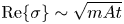 ${\rm Re}\{\sigma \}\sim \sqrt {m At}$ when
  $m\gg 1$, and where the Atwood number
  $At=M/(2+M)$ provides a measure of the relative magnitude of the density jump between inner (particle-rich) and outer (particle-free) regions (
 $0\leq At\leq 1$). When the particles are inertial (
 $St_{\varGamma }\neq 0$) all modes become unstable regardless
  $St_{\varGamma }$ and
  $M\neq 0$, even those with
  $m< m_{cr}$. However, the growth rate of modes
  $m\geq m_{cr}$ is reduced compared with the case
  $St_{\varGamma }=0$. For large-wavenumber modes
  $m\gg 1$, the growth rate approaches
  ${\rm Re}\{\sigma \}\sim \sqrt {m At}(1-2St_{\varGamma }\sqrt {m At}) +O(St_{\varGamma }^2)$. For both inertial and non-inertial particles, the tendency of growth rates to increase with wavenumber
  $m$ suggests that modes that naturally emerge in experiments and simulations will have a high wavenumber. This mode is likely determined by a balance between viscous effects and preferential concentration, although this cannot be ascertained as we have not considered viscous effects in our LSA.
In addition to the LSA, Eulerian–Lagrangian simulations are carried out at  $St_{\varGamma }=0.002$,
  $\mbox {\textit {Re}}=5000$ and mass loadings
  $M= 0.4\unicode{x2013}1$. The simulations are initialized with the base state superimposed with eigenmodes found from LSA. The simulations allow us to explore the transition from linear to nonlinear regimes. During the early evolution of the perturbations, growth rates computed from the perturbation kinetic energy in the Eulerian–Lagrangian simulations show excellent agreement with growth rates predicted by the LSA for modes
  $m= 2\unicode{x2013}6$ and mass loadings
  $M= 0.4\unicode{x2013}1$ (or
  $At= 1/6\unicode{x2013}1/3$). When the flow enters a nonlinear stage, we observe the emergence of a high-wavenumber mode with
  $m\sim 24\unicode{x2013}26$. This mode develops into spiralling arms of number density and vorticity that ultimately cause the breakdown of the initial base state.
One must note that the present study has a key difference from prior investigations of dusty Kolmogorov flow and Rayleigh–Taylor turbulence – a particle-free vortex is always stable. Our study emphasizes that the disperse phase can also be the source of a new instability besides modifying an existing one. The novel instability for a dusty vortex identified here highlights how the feedback force from a disperse phase can induce a breakdown of an otherwise resilient vortical structure.
Funding
The authors acknowledge support from the US National Science Foundation (award no. 2148710, CBET-PMP), and from IIT Madras for the ‘Geophysical Flows Lab’ research initiative under the Institute of Eminence framework.
Declaration of interests
The authors report no conflict of interest.
Author contributions
S.S. and D.J.D. shared equal contributions to the work.


 Open access