


1. Introduction
Laminar–turbulent transition in supersonic boundary layers is an attractive issue due to its relevance to the aerodynamic design of high-speed vehicles. For low environmental perturbations, transition is triggered by the accumulated amplification of normal instability modes (Kachanov Reference Kachanov1994), which are described by the eigenvalue solutions of the compressible Orr–Sommerfeld (O-S) equation system based on the linear stability theory (LST). The simplest setup is a supersonic boundary layer over a flat plate, for which the instability was first studied by Lees & Lin (Reference Lees and Lin1946) and extensively calculated by Mack (Reference Mack1987). This instability was subsequently referred to as the Mack mode. It was reported that as the oncoming Mach number increases, more than one instability mode appears, which are named as the Mack first, second,  $\cdots$, modes according to the ascending order of the frequency. A large number of subsequent numerical works, such as Fedorov (Reference Fedorov2011) and Zhong & Wang (Reference Zhong and Wang2012), confirmed these eigenvalue solutions and showed their spatial evolution in supersonic or hypersonic boundary-layer flows over both flat plates and slender cones with zero angle of attack. From the asymptotic viewpoint, the Mack modes may belong to two distinguished regimes. (1) The first mode with the oblique wave angle (
 $\varTheta \equiv \tan ^{-1}(\beta /\alpha )$ with
  $\alpha$ and
  $\beta$ denoting the streamwise and spanwise wavenumbers, respectively) greater than
  $\tan ^{-1} \sqrt {M^2-1}$ (where
  $M$ denotes the Mach number) shows a viscous-inviscid-interactive nature, described by the triple-deck formalism (Smith Reference Smith1989). (2) The first mode with
  $\varTheta < \tan ^{-1} \sqrt {M^2-1}$ and all higher-order modes are of the inviscid nature (Cowley & Hall Reference Cowley and Hall1990; Smith & Brown Reference Smith and Brown1990). If the slender cone is arranged with even a small angle of attack, the streamlines will be detoured to the leeward surface and the cross-flow (CF) instability appears; see, for instance, a direct numerical simulation (DNS) by Balakumar & Owens (Reference Balakumar and Owens2010) and an experiment of Craig & Saric (Reference Craig and Saric2016). If the cone is rotating about its axis of symmetry, the instability could be more complicated even when the angle of attack is zero. In the recent decades, several works have been directed to the instability mechanisms leading to breakdown of the low-speed boundary layers over rotating discs or cones (Reed & Saric Reference Reed and Saric1989; Kobayashi Reference Kobayashi1994; Saric, Reed & White Reference Saric, Reed and White2003, and references therein). For a rotating-cone boundary layer, a few additional effects may occur simultaneously (Kobayashi Reference Kobayashi1994): (a) the centrifugal force due to the rotation of the fluids; (b) the Coriolis force due to the rotation of the frame; and (c) the CF effect due to the circumferential velocity.
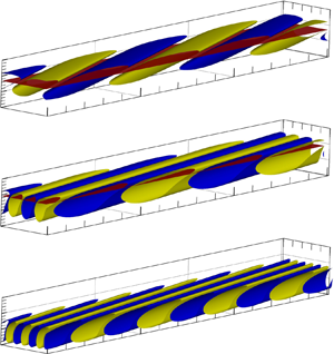
A relevant and the simplest model to demonstrate the rotating effect is a rotating disc placed in an incompressible fluid which is otherwise at rest. Early experiments (Gregory et al. Reference Gregory, Stuart, Walker and Bullard1955; Kobayashi, Kohama & Takamadate Reference Kobayashi, Kohama and Takamadate1980) observed a structure of spiral vortices due to the CF instability, which appears when the Reynolds number  $R$ is approximately
  $9\times 10^4$ (which is also referred to as the critical
  $R$) and eventually leads to transition to turbulence when the
  $R$ reaches approximately
  $3\times 10^5$ (which is also referred to as the transitional
  $R$). Kobayashi et al. (Reference Kobayashi, Kohama and Takamadate1980) and Malik, Wilkinson & Orszag (Reference Malik, Wilkinson and Orszag1981) pointed out that to predict the number of vortices correctly, the effects of the Coriolis force and streamline curvature in the linear stability analysis should be considered. Their predictions of the onset of the CF mode are also rather close to the experimental measurements. Subsequently, Malik (Reference Malik1986) plotted the neutral curves for the stationary CF instability by solving numerically the O-S equation. It was found that the instability modes around the upper-branch neutral curve are governed by the inviscid regime as in Gregory et al. (Reference Gregory, Stuart, Walker and Bullard1955), whereas for those around the lower-branch neutral curve show an important impact of viscosity, whose oblique wave angles
  $\varTheta$ approach the direction perpendicular to the wall shear. Based on the large-
 $R$ asymptotic technique, an in-depth study of the instability mechanisms of the two branches was provided by Hall (Reference Hall1986), who pointed out that for the upper-branch CF instability, the viscosity comes into play only in the critical layer appearing in the second-order balance, whereas the lower-branch instability is a wall mode (showing a triple-deck asymptotic structure), driven by the balance of the viscosity, pressure gradient and Coriolis force in the near-wall region. The asymptotic predictions agree with the O-S solutions (Malik Reference Malik1986) when
  $R$ is sufficiently large. Recently, the receptivity and control of the CF instability in a rotating-disc boundary layer were investigated by Thomas & Davies (Reference Thomas and Davies2021) and Morgan, Davies & Thomas (Reference Morgan, Davies and Thomas2021), respectively.
For a rotating cone in a still flow, the semi-apex angle  $\theta$ becomes a crucial factor influencing its stability characteristics. Early experimental observations by Kobayashi & Izumi (Reference Kobayashi and Izumi1983) revealed that as
  $\theta$ increases, both the critical and transitional Reynolds numbers decrease, indicating a more unstable nature of the flow. Additionally, the direction of the spiral vortices also decreases with
  $\theta$, and for a slender cone, the vortices are almost along the circumference direction. Both phenomena could be predicted by LST. Later, Garrett, Hussain & Stephen (Reference Garrett, Hussain and Stephen2009) extended Hall (Reference Hall1986)'s asymptotic analysis to the rotating-cone configuration, and the instability mechanisms of the lower and upper branches are found to be the same as those for rotating discs. Unfortunately, the asymptotic predictions of the critical Reynolds numbers and the wave angles agree well with the experimental observations only when
  $\theta >40^\circ$; for a more slender cone, the asymptotic predictions show a much later onset of instability and a much greater wave angle than the experimental data. In fact, as
  $\theta$ becomes lower than approximately
  $40^\circ$, the spiral vortex structures change from co-rotating vortices to counter-rotating vortices; therefore, a change over of the dominant instabilities may have occurred. Hussain, Garrett & Stephen (Reference Hussain, Garrett and Stephen2014) attributed the counter-rotating vortices for slender cones to a new instability, namely, the Görtler-type centrifugal instability manifesting as counter-rotating spiral vortices. A short-wavelength asymptotic analysis was performed and the numerical results did provide a better prediction for small
  $\theta$ values. A series of recent experiments confirmed that the CF instability dominates the transition process in rotating broad cones (Kato, Alfredsson & Lingwood Reference Kato, Alfredsson and Lingwood2019a; Kato et al. Reference Kato, Kawata, Alfredsson and Lingwood2019b), whereas the centrifugal instability dominates that in rotating slender cones (Kato et al. Reference Kato, Segalini, Alfredsson and Lingwood2021).
A more complicated but interesting situation is to arrange the rotating cone in an axial flow. An experiment for a slender cone ( $\theta =15^\circ$) (Kobayashi, Kohama & Kurosawa Reference Kobayashi, Kohama and Kurosawa1983) reported that, as the rotating speed increases, the transition onset moves upstream and the instability shows a counter-rotating vortex structure for this semi-apex angle. The impact of the oncoming velocity on the instability in a rotating-slender-cone boundary layer is systematically studied by Hussain et al. (Reference Hussain, Garrett, Stephen and Griffiths2016). It was found that when the ratio of the oncoming velocity to the rotating velocity is large, the instability appears as the Tollmien–Schlichting (TS) mode, which can be described by the triple-deck theory (Smith Reference Smith1979); for a sufficiently small velocity ratio, the centrifugal effect dominates the instability, and the asymptotic analysis, as by Hussain et al. (Reference Hussain, Garrett and Stephen2014), can be extended to reveal this instability mechanism. Increase of the oncoming velocity leads to a stabilising effect. A subsequent experiment (Tambe et al. Reference Tambe, Schrijer, Rao and Veldhuis2021) confirmed its accuracy on the prediction of critical Reynolds number, and the effect of the incident angle was also studied. According to the previous investigations, the different instability regimes in the
  $\theta$–
 $\bar \varOmega$ plane are sketched in figure 1.

Figure 1. Sketch of the instability modes in the  $\theta$–
 $\bar \varOmega$ space, where
  $\bar \varOmega$ is the ratio of the rotation velocity to axial-flow velocity.
The previous investigations on spinning bodies with and without axial flows only focus on incompressible flows. Although the compressible effect is included in a few previous studies (Turkyilmazoglu, Cole & Gajjar Reference Turkyilmazoglu, Cole and Gajjar2000; Turkyilmazoglu Reference Turkyilmazoglu2005, Reference Turkyilmazoglu2007), they were focusing on the rotating discs with stationary compressible background flows, in which only quantitative change of the growth rate is observed. Actually, if the axial (oncoming) flow is increased to a supersonic level, which is related to many engineering applications, more instability regimes may occur or co-exist in certain parameter spaces. First, if the rotating velocity is sufficiently small in comparison with the oncoming supersonic stream, the instability appears as a modified boundary-layer mode for a quasi-two-dimensional (2-D) configuration. Being different from the incompressible and subsonic boundary layers, in which the instability is of the TS regime, the quasi-2-D instabilities in supersonic boundary layers are of the inviscid Mack regime, as pointed out by Lees & Lin (Reference Lees and Lin1946), Smith & Brown (Reference Smith and Brown1990) and Cowley & Hall (Reference Cowley and Hall1990). Second, the rotation of the cone induces a circumferential velocity that is perpendicular to the meridian plane, and so the CF instability may appear if the rotation is sufficiently strong (Balakumar & Reed Reference Balakumar and Reed1991). The effect of the Coriolis force may play an important role in driving the wall-mode instability near the lower-branch neutral point; see Hall (Reference Hall1986) and Butler & Wu (Reference Butler and Wu2018). Third, the rotation also induces a centrifugal force and non-parallelism in the wall-normal direction, which may drive a Görtler-type centrifugal instability as in Hall (Reference Hall1982) and Hussain et al. (Reference Hussain, Garrett, Stephen and Griffiths2016). In this paper, we will provide a systematic study of the instability characteristics of these modes in a supersonic rotating-cone boundary layer.
The rest of this paper is structured as follows. In § 2, we introduce the physical model, mathematical description and the numerical approaches. The numerical results of the base flow is provided in § 3, which are confirmed to be accurate by comparing with the solutions of the full Navier–Stokes (N-S) equations; see Appendix B. The instability analysis is provided in § 4, in which three instability regimes, the modified Mack mode, the cross-flow mode and the centrifugal mode, are investigated in detail. In § 5, we conclude our numerical observations and present remarks and discussions.
2. Problem description and mathematics
2.1. Physical model and governing equations
As shown in figure 2, the physical model to be studied is a sharp rotating cone with an angular velocity  $\varOmega ^*$ inserted into a supersonic stream at zero angle of attack. The semi-apex angle of the cone
  $\theta$ is assumed to be small. After the shock wave, a viscous boundary-layer is formed adjacent to the wall. The body-fitted coordinate system
  $(x^*,y^*,\varphi )$ is employed, where
  $x^*$ and
  $y^*$ are along and perpendicular to the generatrix, respectively, and
  $\varphi$ is the circumferential angle. Throughout this paper, the superscript
  $*$ and subscript
  $e$ denote the dimensional and the boundary-layer edge quantities, respectively.

Figure 2. Sketch of the physical model.
The velocity field  ${\boldsymbol {u}}$ =
  $(u,v,w)$, density
  $\rho$, temperature
  $T$, pressure
  $p$, and dynamic viscosity
  $\mu$ are normalised by
  ${U^{*}_e}$,
  $T^{*}_e$,
  $\rho ^{*}_e$,
  $\rho ^{*}_e{U^{*2}_e}$ and
  $\mu ^*_e$, respectively, where
  ${U^{*}_e}$,
  $T^{*}_e$ and
  $\rho ^{*}_e$ are the velocity, temperature and density at the boundary-layer edge. The unit length is taken to be the characteristic length of the boundary layer,
  $\delta ^* = \sqrt {{{L^*{\mu _e ^{*} }}}/{{{\rho _e ^{*} }{U_e ^{*}}}}}$, where
  $L^*$ measures the distance to the leading edge of the cone. Thus, the coordinate system and time are normalised as
  $( {x,y} ) = {{( {{x^*},{y^*}} )} /{{\delta ^*}}}$ and
  $t = {{{t^*}{\delta ^*}} / {U_e ^*}}$, respectively. The flow system is governed by three characteristic parameters, the Reynolds number
  $R = {{\rho _e ^*U_e ^*{\delta ^*}}}/{{\mu _e ^*}}$, the Mach number
  $M = {{U_e ^*}}/{{a_e ^*}}$ and the dimensionless angular velocity
  $\varOmega = {{{\varOmega ^*}{\delta ^*} }}/{{U_e ^*}}$, where
  $a^{*}_{e}$ is the sound speed at the edge of the boundary layer. Additionally, the ratio of the rotating velocity at
  $x^* = L^*$ to the boundary-layer edge velocity
  $U_{e}^{*}$ is defined by
  $\bar \varOmega ={\varOmega ^* L^* \sin \theta }/{U^{*}_{e}}= \varOmega R \sin \theta$. In this paper, we take
  $\bar \varOmega = O(1)$, then
  $\varOmega$ is only of
  $O(R^{-1})$.
The dimensionless compressible N-S equations in the rotating frame are (Towers Reference Towers2013)
 \begin{gather} \frac{{\partial \rho }}{{\partial t}} + \boldsymbol{\nabla} \boldsymbol{\cdot} \left( {\rho {\boldsymbol{u}}} \right) = 0, \end{gather}
 \begin{gather}\rho \left[ {\frac{{{\rm D}{\boldsymbol{u}}}}{{{\rm D}t}} + 2 \boldsymbol{\varOmega} \times {\boldsymbol{u}} + \boldsymbol{\varOmega} \times \left( {\boldsymbol{\varOmega} \times {\boldsymbol{r}}} \right)} \right] ={-} \boldsymbol{\nabla} p + \frac{1}{R}\left[ {2\boldsymbol{\nabla} \boldsymbol{\cdot} \left( {\mu {\boldsymbol{S}}} \right) - \frac{2}{3}\boldsymbol{\nabla} \left( {\mu \boldsymbol{\nabla} \boldsymbol{\cdot} {\boldsymbol{u}}} \right)} \right],\quad \end{gather}
 \begin{gather}\frac{1}{\gamma }\rho \frac{{{\rm D}T}}{{{\rm D}t}} - \frac{{\gamma - 1}}{\gamma }T\frac{{{\rm D}\rho }}{{{\rm D}t}} = \frac{1}{{PrR}}\boldsymbol{\nabla} \boldsymbol{\cdot} \left( {\mu \boldsymbol{\nabla} T} \right) + \frac{{\left( {\gamma - 1} \right){M^2}}}{{R}}\left[ {2\mu {\boldsymbol{S}}:{\boldsymbol{S}} - \frac{2}{3}\mu {{\left( {\boldsymbol{\nabla} \boldsymbol{\cdot} {\boldsymbol{u}}} \right)}^2}} \right], \end{gather}
 \begin{gather}{p} = \frac{{\rho }{T}}{\gamma {M}^2}, \end{gather}
where  ${\boldsymbol {S}} = {{[ {\boldsymbol {\nabla } {\boldsymbol {u}} + {{( {\boldsymbol {\nabla } {\boldsymbol {u}}} )}^{\rm T}}} ]} / 2}$ is the rate of strain tensor,
  $Pr$ is the Prandtl number,
  $\boldsymbol {\varOmega }= { \varOmega } ( \cos \theta,- \sin \theta,0 )$ is the angular velocity vector,
  $\gamma$ is the ratio of the specific heats and
  ${{\rm D}}/{{\rm D}t} = {\partial }/{\partial t} + \boldsymbol {u} \boldsymbol {\cdot } \boldsymbol {\nabla }$ denotes the material derivative. Sutherland's viscosity law is assumed, namely,
  $\mu (T)=(1+ {C})T^{{3}/{2}}/(T+ { C})$ with
  ${C}=110.4/{T_e}$. In addition,
  ${\boldsymbol {r}}=r(\sin \theta, \cos \theta, 0)$ is the position vector with
  $r$ being the distance to the rotating axis,
 \begin{equation} r=x \sin \theta + y \cos \theta . \end{equation}
The instantaneous flow field  $\phi$ can be decomposed into a steady base flow
  $\varPhi _B$ and an infinitesimal perturbation
  $\tilde \phi$,
 \begin{equation} \phi = ( U_B, R^{{-}1} V_B, W_B,\rho_B, T_B, P_B) + {\mathcal{E}} \tilde \phi, \end{equation}
where  $\phi \equiv (u,v,w, \rho, T,p)$, and
  ${\mathcal {E}} \ll 1$ measures the amplitude of the perturbation.
2.2. Base flow
Because the base flow varies slowly with  $x$, we introduce a slow variable,
 \begin{equation} X=R^{{-}1}x, \end{equation}
such that  $\partial _ X \varPhi _B= O(1)$. Considering that the base flow is steady and invariant with
  $\varphi$, the N-S system (2.1) is reduced to the boundary-layer equations
 \begin{gather} \frac{{\partial \left( {\rho_B U_B \bar r} \right)}}{{\partial X}} + \frac{{\partial \left( {\rho_B V_B \bar r} \right)}}{{\partial y}} = 0, \end{gather}
 \begin{gather}\rho_B \left[ {U_B\frac{{\partial U_B}}{{\partial X}} + V_B\frac{{\partial U_B}}{{\partial y}} - X{\bar \varOmega ^2}{{\left( {\bar W_B + 1} \right)}^2}} \right] = \frac{\partial }{{\partial y}}\left( {\mu_B \frac{{\partial U_B}}{{\partial y}}} \right), \end{gather}
 \begin{gather}\rho_B \left[ {U_B\frac{{\partial \bar W_B}}{{\partial X}} + V_B\frac{{\partial \bar W_B}}{{\partial y}} + \frac{{2U_B\left( {\bar W_B + 1} \right)}}{X}} \right] = \frac{\partial }{{\partial y}}\left( {\mu_B \frac{{\partial \bar W_B}}{{\partial y}}} \right), \end{gather}
 \begin{gather}\rho_B \left( {U_B\frac{{\partial T_B}}{{\partial X}} + V_B\frac{{\partial T_B}}{{\partial y}}} \right) = \left( {\gamma - 1} \right)M^2\mu_B \left[ {{{\left( {\frac{{\partial U_B}}{{\partial y}}} \right)}^2} + {X^2}{\bar \varOmega ^2}{{\left( {\frac{{\partial \bar W_B}}{{\partial y}}} \right)}^2}} \right] \nonumber\\ + \frac{1}{{{Pr}}}\left[ {\frac{\partial }{{\partial y}}\left( {\mu_B \frac{{\partial T_B}}{{\partial y}}} \right)} \right] ,\end{gather}
 \begin{gather}\rho_B T_B =1, \end{gather}
where  $\bar W_B={W_B}/({ \bar \varOmega X })$,
  $\bar r= X \sin \theta$ and the
  $O(R^{-1})$ terms are neglected. According to the potential-flow analysis (Anderson Reference Anderson1990), for a supersonic flow past a sharp cone, the potential flow after the shock shows a conic-flow feature, for which all the physical quantities stay unchanged along each line originating from the cone tip. Therefore, the pressure gradient is negligible to leading order. The no-slip, non-penetration and isothermal boundary conditions are applied at the wall,
 \begin{equation} (U_B, V_B, \bar W_B, T_B)=(0,0,0,T_w), \quad \text{at} \ y=0, \end{equation}
where  $T_w$ is the dimensionless wall temperature. Note that for an adiabatic wall, we simply change the wall temperature condition to
  ${{\partial {T_B}} / {\partial y = 0}}$. The upper boundary conditions read
 \begin{equation} (\rho_B, U_B, \bar W_B, T_B)\rightarrow(1,1,-1,1), \quad \text{as} \ y \to \infty. \end{equation}
The Mangler transformation is introduced to regularise the system (2.5) into a planar form,
 \begin{equation} \left. \begin{aligned} & \bar X = \int_0^X {{\bar r^2}\,{\rm d}\hat X} = \frac{1}{3}{X^3}{\sin ^2}\theta, \quad \bar y =\bar ry = X \sin \theta y,\\ & \bar V_B = \frac{1}{\bar r}\left( {V_B + \frac{1}{\bar r}\frac{{{\rm d} \bar r}}{{{\rm d}X}}y U_B} \right) = \frac{1}{X \sin \theta} \left( {V_B + \frac{y}{X} U_B} \right). \end{aligned} \right\} \end{equation}
Additionally, the Dorodnitzyn–Howarth transformation, as has been used for the compressible Blasius solution, is applied,
 \begin{equation} \eta = \frac{1}{{\sqrt {\bar X} }}\int_0^{\bar y} {\rho_B \,{\rm d}\hat y} ,\quad \tilde V_B = \sqrt {\bar X} \rho_B \bar V_B + \bar X U_B\frac{{\partial \eta }}{{\partial \bar X}}. \end{equation}
Thus, the boundary-layer equations (2.5) are recast to
 \begin{gather} \bar X \frac{{\partial U_B}}{{\partial \bar X }} + \frac{{\partial \tilde V_B}}{{\partial \eta }} + \frac{1}{2}U_B = 0, \end{gather}
 \begin{gather}\bar X U_B\frac{{\partial U_B}}{{\partial \bar X }} + \tilde V_B\frac{{\partial U_B}}{{\partial \eta }} - \frac{1}{3}{\bar \varOmega ^2}{\left( {\bar W_B + 1} \right)^2}{\left( {\frac{{3\bar X }}{{{{\sin }^2}\theta }}} \right)^{{2}/{3}}} = \frac{\partial }{{\partial \eta }}\left( {\frac{\mu_B }{T_B}\frac{{\partial U_B}}{{\partial \eta }}} \right), \end{gather}
 \begin{gather}\bar X U_B\frac{{\partial \bar W_B}}{{\partial \bar X }} + \tilde V_B\frac{{\partial \bar W_B}}{{\partial \eta }} + \frac{2}{3}U_B \left( {\bar W_B + 1} \right) = \frac{\partial }{{\partial \eta }}\left( {\frac{\mu_B }{T_B}\frac{{\partial \bar W_B}}{{\partial \eta }}} \right), \end{gather}
 \begin{gather}\bar X U_B\frac{{\partial T_B}}{{\partial \bar X }} + \tilde V_B\frac{{\partial T_B}}{{\partial \eta }} = \left( {\gamma - 1} \right){M^2}\frac{\mu_B }{T_B}\left[ {{{\left( {\frac{{\partial U_B}}{{\partial \eta }}} \right)}^2} + {{\left( {\frac{{3\bar X }}{{{{\sin }^2}\theta }}} \right)}^{{2}/{3}}}{\bar \varOmega ^2}{{\left( {\frac{{\partial \bar W_B}}{{\partial \eta }}} \right)}^2}} \right]\nonumber\\ +\frac{1}{\textit{Pr} }\frac{\partial }{{\partial \eta }}\left( {\frac{\mu_B }{T_B}\frac{{\partial T_B}}{{\partial \eta }}} \right), \end{gather}
and the boundary conditions are imposed as follows,
 \begin{gather} (U_B, \tilde V_B, \bar W_B, T_B)=(0,0,0,T_w), \quad \text{at} \ y=0, \end{gather}
 \begin{gather}(\rho_B, U_B, \bar W_B, T_B)\rightarrow(1,1,-1,1), \quad \text{as} \ y \to \infty. \end{gather}
 For cases without rotation, i.e.  $\bar \varOmega =0$, and the boundary-layer equations (BLEs) (2.10) with (2.11) admit a self-similar solution, known as the compressible Blasius solution. However, for a rotating case, (2.10) has to be solved numerically by a marching scheme due to its parabolic nature. Note that in the limit of
  $\bar X \to 0$,
  $U_B$,
  $W_B$ and
  $T_B$ are finite and much smaller than
  $\ln \bar X$, therefore, the system (2.10) is reduced to a group of ordinary differential equations,
 \begin{gather} \tilde {V_B}^{\prime} + \frac{1}{2}U_B = 0, \end{gather}
 \begin{gather}\tilde V_B U_{B}^{\prime} - \left( {\frac{\mu_B }{T_B} U_{B}^{\prime} }\right)^{\prime}=0, \end{gather}
 \begin{gather}\tilde V_B W_{B}^{\prime} + \frac{2}{3}u\left( {\tilde W_B + 1} \right) = \left( {\frac{\mu_B }{T_B} W_{B}^{\prime} }\right)^{\prime}, \end{gather}
 \begin{gather}\tilde V_B T_B^{\prime} = \frac{1}{\textit{Pr} } \left( {\frac{\mu_B }{T_B} T_{B} ^{\prime}} \right)^{\prime} + \left( {\gamma - 1} \right){M^2}\frac{\mu_B }{T_B} {U_B^{\prime}}^{2}, \end{gather}
whose boundary conditions are the same as (2.11). In what follows, a prime denotes the derivative with respect to its argument. The system (2.12) can be solved by the fourth-order Runge–Kutta integrative method, whose solution is set as the inflow boundary condition of (2.10) at  $\bar X=0$. The system (2.10) is solved using the third-order backward finite differential scheme. At each location, the flow field is described by a group of ordinary differential equations (ODEs) of
  $\eta$, which is solved by the Chebyshev collocation method. The numerical method is the same as that of Pruett (Reference Pruett1994), in which the base flow for a swept-wing boundary layer without the Coriolis-force effect was studied.
2.3. Linear stability analysis
Based on the base flow at  $X=1$ or
  $x=R$, we perform the linear stability analysis. Under the local parallel-flow assumption, the perturbation
  $\tilde \phi$ is expressed in the travelling-wave form,
 \begin{equation} \tilde \phi= \hat \phi \left( y \right){\exp({\text{i} \left( {\alpha x + \beta r_0 \varphi - \omega t} \right)})}+ \text{c.c.}, \end{equation}
where  $\textrm {i}\equiv \sqrt {-1}$,
  $\hat \phi$ is the perturbation profile,
  $\alpha$ the streamwise wavenumber,
  $\beta$ the spanwise wavenumber,
  $\omega$ the frequency,
  $r_0=x \sin \theta$ denotes the radius of the wall and
  $\textrm {c.c.}$ represents the complex conjugate. All the eigenvalues
  $\alpha$,
  $\beta$ and
  $\omega$, could be complex, but we are interested in either the temporal mode for which only
  $\omega = \omega _r + \textrm {i} \omega _i$ is complex with its imaginary part representing the growth rate, or the spatial mode for which only
  $\alpha = \alpha _r + \textrm {i} \alpha _i$ is complex with the opposite of its imaginary part representing the growth rate. Substituting (2.3) and (2.13) into (2.1) and retaining the
  $O({\mathcal {E}})$ terms, we arrive at the linear homogeneous system in the rotating frame,
 \begin{gather} \tilde S \hat \rho + \rho_{B,y} \hat v + \rho_B \mathscr{D} = 0, \end{gather}
 \begin{gather}\rho_B \left( { \tilde S \hat u + {U_{B,y}}\hat v } \right) + \text{i}\alpha \hat p ={\mathcal{C}}_{x}+ {\mathcal{R}}_{x} + {\mathcal{T}}_{x}/R, \end{gather}
 \begin{gather}\rho_B { \tilde S \hat v } + \hat p^{\prime} ={\mathcal{C}}_{y}+ {\mathcal{R}}_{y} + {\mathcal{T}}_{y}/R, \end{gather}
 \begin{gather}\rho_B \left( { \tilde S \hat w + W_{B,y} \hat v } \right) + \text{i} \tilde \beta \hat p ={\mathcal{C}}_{\varphi}+ {\mathcal{R}}_{\varphi} + {\mathcal{T}}_{\varphi}/R, \end{gather}
 \begin{gather}\rho_B \left( { \tilde S \hat T + T_{B,y} \hat v} \right) + (\gamma-1)\mathscr{D} = \gamma \left({\gamma - 1} \right) M^2 {\mathcal{T}}_{e}/R, \end{gather}
 \begin{gather}\frac{{\hat \rho }}{{\rho_B}} + \frac{{\hat T}}{{T_B}}= \gamma M^2 \hat p , \end{gather}
where  $\tilde S=\textrm {i}({\alpha U_B + \tilde \beta W_B - \omega })$,
  $\mathscr {D}= (\textrm {i}\alpha \hat u + \hat v^{\prime }+ \textrm {i} \tilde \beta \hat w + \bar \kappa \hat v + \tan \theta \bar \kappa \hat u)$ represents the divergence of the velocity,
  $\tilde \beta = \beta /(1+ y \kappa )$,
  $\bar \kappa = \kappa /(1+y \kappa )$, and
  $\kappa =\cot \theta /x \equiv \cot \theta / R$ is the curvature in the circumferential direction. Here,
  ${\mathcal {T}}_{x}$,
  ${\mathcal {T}}_{y}$,
  ${\mathcal {T}}_{\varphi }$ and
  ${\mathcal {T}}_{e}$ denote the viscous terms in the
  $x$-momentum,
  $y$-momentum,
  $\varphi$-momentum and energy equations which can be deduced readily from Appendix A. Here,
  ${\mathcal {R}}_x$,
  ${\mathcal {R}}_y$ and
  ${\mathcal {R}}_\varphi$ denote the terms associated with the rotation in the momentum equations,
 \begin{gather} {\mathcal{R}}_x ={\mathcal{R}}_{x1}+{\mathcal{R}}_{x2}\equiv\left(2\varOmega \sin \theta ( \rho_B \hat w + W_B \hat{\rho})\right) + \left(\varOmega^2\sin\theta r \hat{\rho} \right), \end{gather}
 \begin{gather}{\mathcal{R}}_y ={\mathcal{R}}_{y1} +{\mathcal{R}}_{y2} \equiv\left( 2\varOmega \cos \theta ( \rho_B \hat w + W_B \hat{\rho})\right) +\left( \varOmega^2 \cos \theta r \hat{\rho} \right), \end{gather}
 \begin{gather}{\mathcal{R}}_{\varphi} = {\mathcal{R}}_{\varphi 1}+ {\mathcal{R}}_{\varphi 2} \equiv{-}\left(2 \varOmega \cos \theta \rho_B \hat v + 2 \varOmega\sin \theta ( \rho_B \hat u + U_B \hat{\rho} )\right)-\left(0\right), \end{gather}
where the first and second terms in the big brackets on the right-hand side of each equation denote the impacts of the Coriolis and centrifugal forces, respectively. The terms  ${\mathcal {C}}_{x}$,
  ${\mathcal {C}}_{y}$ and
  ${\mathcal {C}}_{\varphi }$ in the momentum equations are associated with the curvature, which read
 \begin{gather} {\mathcal{C}}_{x}=2\tan \theta \bar \kappa \rho_B W_{B} \hat w+\tan \theta \bar \kappa W_{B}^{2} \hat \rho, \end{gather}
 \begin{gather}{\mathcal{C}}_{y}= 2 \bar \kappa \rho_B W_B\hat w +\bar \kappa {W_B^2} \hat \rho , \end{gather}
 \begin{gather}{\mathcal{C}}_{\varphi} ={-}\rho_B \bar \kappa (\tan \theta U_B \hat w+ W_B \hat{v}) -\tan \theta W_B( \bar \kappa +\kappa )(U_B \hat{\rho}+\rho_B \hat{u}). \end{gather}
 There may be a number of instability mechanisms governed by the linear system (2.14). First, if the rotation rate is sufficiently small, the instability will be the classical Mack mode in quasi-2-D boundary-layer flows, including both the inviscid mode for small oblique wave angles and viscous mode for large oblique wave angles. As  $\varOmega$ increases, the cross-flow (CF) effect may play an important role, leading to the occurrence of the CF instability. Additionally, if (2.15b) and (2.16b) are combined, then (2.14c) is rewritten as
 \begin{equation} \rho_B \tilde S \hat v + \hat p^{\prime} = {\mathcal{T}}_{y}/R + \cos \theta\left[ \frac{2\rho_B(W_B+ \varOmega r) \hat w }{r}+ \frac{{(W_B+\varOmega r)^2\hat \rho}}{r} \right]. \end{equation}
Since  $W_B + \varOmega r$ is the circumferential velocity in a stationary frame, the second term on the right-hand side appears as the centrifugal effect, which is a reminiscence of Görtler instability on a concave wall. For such an instability, the asymptotic analysis in Hall (Reference Hall1982) uncovered that the leading-order balance is between the centrifugal effect and viscosity, while the wall-normal pressure gradient appears in the second-order balance. The centrifugal effect is usually measured by the Taylor number
  $T_a = \cot \theta \bar \varOmega ^2$ (Hall Reference Hall1982; Hussain et al. Reference Hussain, Garrett, Stephen and Griffiths2016), defined as the ratio of the centrifugal effect to the viscous effect. Considering
  $r \approx r_0$ for a sufficiently downstream location, (2.17) can be recast to
 \begin{equation} \frac{R}{T_a} \rho_B \tilde S \hat v + \frac{R}{T_a} \hat p^{\prime} =\left[ 2\rho_B(\bar W_B+ 1) \frac{ \hat w }{\bar \varOmega} + {{(\bar W_B+1)^2\hat \rho}} \right] + \frac{1}{T_a} {\mathcal{T}}_{y}. \end{equation}
From (2.18), we know that the increase of  $R$ leads to weakened centrifugal and viscous effects, producing a stabilising effect on the centrifugal mode; however, increase of
  $\bar \varOmega$ (
 $T_a$) promotes the centrifugal effect. A systematic study on this centrifugal instability will be demonstrated in § 4.4.
The numerical scheme to solve the linear stability system will be based on the method given by Malik (Reference Malik1990), in which the system is expressed in terms of a group of first-order ODEs. We introduce a new unknown vector  $\hat \phi _{OS} = {( {\hat u,\hat v,\hat w,\hat T,\hat f,\hat q,\hat g,\hat h} )}$, with
 \begin{equation} \left. \begin{aligned} & \hat f = {{\hat u}_y} + U_{B,y}\, {{ \mu }_{B,T}}\hat T/ \mu_B, \quad \hat q ={-} \hat p/ \mu_B + \tfrac{4}{3} \mathscr{D},\\ & \hat g = {{\hat w}_y} - \bar \kappa \hat w + (W_{B,y}- \bar \kappa W_B)\, {{ \mu }_{B,T}}\hat T/ \mu_B, \quad \hat h = {{\hat T}_y} + {{ \mu }_{B,T}}{T_{B,y}}\hat T/ \mu_B. \end{aligned} \right\} \end{equation}
Then, (2.14) is recast to the compressible O-S equation system,
 \begin{equation} {L_{OS}}\left( {d_y;\omega ,\alpha ,\beta ,R } \right)\hat \phi_{OS} \equiv \left ( {\boldsymbol{I}} \frac{{\rm d}}{{\rm d} y}- \boldsymbol{\mathsf{A}} \right) \hat \phi_{OS} = 0, \end{equation}
where  $L_{OS}$ denotes the O-S operator and the coefficient matrix
  $\boldsymbol{\mathsf{A}}$ is introduced in Appendix A. In principle, (2.20) is equivalent to equation (2.36) in Malik (Reference Malik1990), but in the coefficient matrix
  $\boldsymbol{\mathsf{A}}$, the terms associated with the second-order derivative of the base flow do not appear. For the discrete modes, the homogeneous boundary conditions are imposed,
 \begin{equation} (\hat u, \hat v, \hat w, \hat T ) = 0, \quad \text{at} \ y = 0, \quad (\hat u, \hat v, \hat w, \hat T ) \to 0, \quad \text{as} \ y \to \infty. \end{equation}
Thus, the system (2.20) with (2.21) forms an eigenvalue problem.
If the instability is of the inviscid nature, and the Coriolis, centrifugal and curvature effects do not appear in the leading-order balance, then (2.20) can be approximated by the Rayleigh equation, which is expressed as a second-order ODE,
 \begin{equation} {L_{R}}\left( {d_y;\omega ,\alpha ,\beta } \right)\hat \phi_{R} = 0, \end{equation}
where  $\hat \phi _{R}=(\hat v, \hat p)$, and
  $L_R$ denotes the Rayleigh operator,
 \begin{align} {L_R}\left( {{d_y};\omega ,\alpha ,\beta } \right) \equiv {\boldsymbol{I}} \frac{{\rm d}}{{{\rm d} y}} - \left( {\begin{array}{cc} {\left( {{\rm i}\alpha {U_{B,y}} + {\rm i}\beta {W_{B,y}}} \right)/\tilde S} & {\left[ { - {M^2}{{\tilde S}^2} - {T_B}\left( {{\alpha ^2} + {\beta ^2}} \right)} \right]/\tilde S}\\ { - \tilde S/{T_B}} & 0 \end{array}} \right) .\end{align}
For both linear systems (2.20) and (2.22), the fourth-order compact finite-difference scheme as used by Malik (Reference Malik1990) is employed, and the code for flat-plate configurations has been applied in a few of our previous works (Wu & Dong Reference Wu and Dong2016; Dong, Liu & Wu Reference Dong, Liu and Wu2020; Song, Zhao & Huang Reference Song, Zhao and Huang2020; Dong & Zhao Reference Dong and Zhao2021; Li & Dong Reference Li and Dong2021; Zhao & Dong Reference Zhao and Dong2022).
3. Numerical solutions of the base flow over a rotating cone
In this paper, the computational conditions are chosen from the experimental works (Sturek et al. Reference Sturek, Dwyer, Kayser, Nietubicz, Reklis and Opalka1978; Klatt, Hruschka & Leopold Reference Klatt, Hruschka and Leopold2012), although they were not focusing on the flow instability. Table 1 lists the detailed computational parameters. Solving (2.10) with (2.11) and (2.12), we obtain the steady base flow for different  $\bar \varOmega$ values. The calculations are confirmed to be sufficiently accurate by comparing with the full N-S solutions, as shown in Appendix B. The wall-normal profiles of
  $U_B$,
  $V_B$,
  $W_B$ and
  $T_B$ are shown in figure 3(a–c). In the boundary layer,
  $U_B$,
  $|W_B|$ and
  $T_B$ increase with
  $\bar \varOmega$ monotonically. Because the rotation velocity induces an additional kinetic energy of the external stream in the rotating frame, more internal energy is transferred as the wall is approached for a higher rotating rate, leading to a higher temperature in the near-wall region and its gradient at the isothermal wall. The wall shears of
  $U_B$ and
  $|W_B|$ also increase with
  $\bar \varOmega$, as indicated in figure 3(d).

Figure 3. Base flow for different  $\bar \varOmega$ at
  $X=1$: (a)
  $U_B$ and
  $V_B$; (b)
  $W_B$; (c)
  $T_B$; (d) the wall shear of
  $U_B$,
  $W_B$ and
  $T_B$.
Table 1. Parameters characterising the base flow.
The velocities along ( $U_p$) and perpendicular (
 $U_c$) to the direction of the streamline at the boundary-layer edge are defined as
 \begin{equation} U_p=U_B \cos \varPhi_e+W_B \sin \varPhi_e, \quad U_c={-}U_B \sin \varPhi_e+W_B \cos \varPhi_e, \end{equation}
where the oblique angle of the streamline at the boundary-layer edge  $\varPhi _e \equiv \tan ^{-1} (W_e)$, with
  $W_e$ being the circumferential velocity at the boundary-layer edge. Figure 4 shows the wall-normal profiles of
  $U_p$ and
  $U_c$ for different
  $\bar \varOmega$ values. Here,
  $U_p$ increases with
  $\bar \varOmega$ monotonically since
  $W_B$ induced by the rotation is increasing. The velocity in the cross-flow direction
  $U_c$ is zero at
  $y=0$ and
  $y \to \infty$, and two inflectional points appear for
  $\bar \varOmega \neq 0$. Especially, for
  $\bar \varOmega =1.5$,
  $U_c$ crosses the zero line at
  $y\approx 2.38$, and the lower inflectional point shifts towards the boundary-layer edge.

Figure 4. Wall-normal profiles of (a)  $U_p$ and (b)
  $U_c$ at
  $X=1$ for different
  $\bar \varOmega$ values.
For an axisymmetric configuration,  $\bar \varOmega =0$, the base flow satisfies the similarity solution, for which the displacement thickness,
  $\delta _u=\int _0^\infty {( {1 -\rho _B U_B} )}\, {\textrm {d} y}$, grows like
  $x^{{1}/{2}}$. When a rotation is imposed,
  $\bar \varOmega >0$, the displacement feature may be changed because the self-similar state is not valid any more, as indicated by (2.10). Simultaneously, a displacement of the circumferential momentum appears due to the rotation, leading to a circumferential displacement thickness, defined by
  ${\delta _w} = \int _0^\infty {( {1 - \rho _B {{ W_B}}/{{{W_e }}}} )}\, {\textrm {d} y}$. Figure 5(a) shows the streamwise evolution of
  $\delta _u$ and
  $\delta _w$, both of which grow like
  $x^{{1}/{2}}$ overall, but
  $\delta _w < \delta _u$ slightly for all streamwise locations. As
  $\bar \varOmega$ increases, the evolution of
  $\delta _u$ deviates from the axisymmetric configuration slightly, especially in the downstream region. A further demonstration of such a deviation is to plot the normalised thickness
  ${{{\delta _u}}}/({{{\delta _u}| {_{\varOmega = 0}} }})$, as shown in figure 5(b). For
  $\bar \varOmega \leq 1.0$,
  $\delta _u/\delta _u|_{\varOmega =0}$ decreases with
  $x$ monotonically, indicating a smaller displacement effect of the boundary layer. This is because
  $U_B$ in the boundary layer increases with
  $\bar \varOmega$, as shown in figure 3(a), which leads to a reduction of the displacement of the fluids. Interestingly, for a relatively large
  $\bar \varOmega$, i.e.
  $\bar \varOmega =1.5$, the deviation starts to reduce after
  $X \approx 0.75$. This is because a larger
  $\bar \varOmega$ leads to a higher temperature and hence a lower density in the downstream boundary layer, producing an additional compensating effect for the displacement of the fluids.

Figure 5. Streamwise evolution of the (a) displacement thicknesses  $\delta _u$ and
  $\delta _w$ and the (b) normalised displacement thickness
  ${{{\delta _u}}}/({{{\delta _u}| {_{\varOmega = 0}}}})$ for different
  $\bar \varOmega$.
4. The linear instability of a rotating-cone boundary layer
For a boundary layer over a rotating cone, there are two factors influencing its instability characteristics compared to that over a non-rotating cone: (1) the circumferential velocity  $W_B$; (2) the combined effect of the curvature, Coriolis force and centrifugal force.
The first factor may introduce a cross-flow effect to the instability equation, and its effect depends on the projection of the base-flow velocity vector along the direction perpendicular to the instability wave angle
 \begin{equation} \varTheta = \tan ^{{-}1}(\gamma_f),\quad \text{with }\gamma_f = \beta / \alpha_{r}. \end{equation}
 For convenience, we project the velocity vector  $(U_B,W_B)$ into
  $(\tilde U,\tilde W)$, with
 \begin{equation} \left. \begin{aligned} & \tilde U = \frac{{\alpha_{r} U_B + \beta W_B}}{{\tilde a}} = \text{sgn} (\alpha_r )\frac{{U_B + {\gamma _f} W_B}}{{\sqrt {1 + \gamma _f^2} }},\\ & \tilde W=\frac{{-\beta U_B + \alpha_{r} W_B}}{{\tilde a}} = \text{sgn} (\alpha_r )\frac{{- \gamma _f U_B +W_B }}{{\sqrt {1 + \gamma _f^2} }}, \end{aligned} \right\} \end{equation}
where  $\tilde \alpha = \sqrt {{\alpha _{r} ^2} + {\beta ^2}}= |\alpha _{r}| \sqrt {1 + \gamma _f ^2}$. Here,
  $\tilde U$ is referred to as the ’effective velocity’ by Hall (Reference Hall1986). In (4.2), the effect of curvature is neglected because
  $\kappa \ll 1$. For convenience, we introduce
  $c = \omega / \tilde \alpha$, whose real part
  $c_r$ denotes the phase speed along the direction of the wave vector. Figure 6(a,b) show the profiles of
  $\tilde U$ for different
  $\gamma _f$ for
  $\bar \varOmega =0.3$, where the generalised inflectional point (GIP) (defined by the location where
  $(\rho _B \tilde U_{y})_y =0$) and the nominal boundary-layer thickness
  $\delta _{99}$ (defined by the position where
  $U_B =0.99 U_e$) are marked. As
  $\gamma _f$ decreases from 0 to
  $-\infty$, the effective velocity
  $\tilde U$ changes from
  $U_B$ to
  $-W_B$ gradually, and the location of the GIP (
 $y_c$) moves towards the wall with the effective velocity at
  $y_c$,
  $\tilde U_c\equiv \tilde U(y_c)$, decreasing monotonically. Because the
  $U_B$ and
  $W_B$ profiles have opposite signs, the
  $\tilde U$ values at the potential-flow region increase with
  $\gamma _f$ for
  $\gamma _f <0$, but decrease with
  $\gamma _f$ for
  $\gamma _f >0$. Particularly, when
  $\gamma _f$ is close to
  $-1 / W_e\approx 3.3$,
  $\tilde U$ outside of the boundary layer almost vanishes and the effective velocity inside the boundary layer, including
  $\tilde U_c$, is rather small. It is indicated from the balance of the convective and unsteady terms in (2.14) that an instability with quasi-zero frequency may appear, since the real part of
  $\tilde S$ is approximated by
  $\textrm {i} (\tilde \alpha \tilde U - \omega )$. The implication is that a quasi-stationary CF instability driven by the rotation may appear when
  $\varTheta$ is close to
  $\tan ^{-1}(-W_{e}^{-1})$.

Figure 6. Wall-normal profiles of  $\tilde U$ for different
  $\gamma _f$. (a)
  $\gamma _f=-\infty,\ -4,\ -3,\ -2,\ -1,\ 0$. (b)
  $\gamma _f=$1, 2 , 3, 4,
  $\infty$. The vertical black dashed lines in panels (a,b) indicate the location of the nominal boundary-layer edge (
 $\delta _{99}$); the pink dots mark the locations of GIPs.
The second factor comes into play when the rotation rate is sufficiently strong, leading to a typical centrifugal instability as represented in (2.17) or its simplified form (2.18). Actually, the centrifugal effect is determined by the rotation velocity in the stationary frame  $\bar W_B+1$, which reduces from its maximum (unity) at the wall to zero at the boundary-layer edge, indicating its dominant role in the near-wall region. This centrifugal instability has been observed and analysed in a few incompressible boundary layers over slender spinning bodies (Kobayashi & Izumi Reference Kobayashi and Izumi1983; Hussain et al. Reference Hussain, Garrett and Stephen2014, Reference Hussain, Garrett, Stephen and Griffiths2016).
In this paper, we will probe if the aforementioned cross-flow and centrifugal instabilities could exist in the supersonic boundary layers over a rotating cone. Additionally, if the rotation rate is small, the Mack mode could also appear. For demonstration, the following analysis will be mainly based on the base-flow profile for  $\bar \varOmega = 0$, 0.3, 0.75, 1 and 1.25 at
  $X=1$ and
  $R=2000$, but
  $R$ may be changed to probe its effect on instability.
4.1. Overall solutions of the instability system
It has been demonstrated by Mack (Reference Mack1987) that there could be a multiplicity of unstable modes in supersonic boundary layers, i.e. the first, second,  $\cdots$, and the higher-order unstable modes only appear when
  $M$ is sufficiently high. For the present oncoming Mach number, only the unstable first mode exists. The neutral curves in the
  $\omega$–
 $\varTheta$ and
  $\omega$–
 $\beta$ planes are compared in figure 7(a,b), respectively. For
  $\bar \varOmega =0$, the instability mode is the Mack first mode, and the neutral curve is symmetric about the
  $\varTheta =0$ (or
  $\beta =0$) line. When
  $\bar \varOmega$ is increased to 0.3, the neutral curve, shown by the red lines, is distorted to an asymmetric nature, and the size of the unstable zone in the second quadrant is reduced but is enlarged when
  $\beta$ (or
  $\varTheta$) is positive. Overall, the difference between the two neutral curves is not large for most of the
  $\varTheta$ or
  $\beta$ values. Therefore, the majority of this mode is referred to as the modified Mack mode (MMM). However, the neutral curve for
  $\bar \varOmega =0.3$ includes a part of the
  $\omega =0$ line for positive
  $\beta$ values, indicating the appearance of a stationary mode, which is reminiscent of the cross-flow instability. When the
  ${\mathcal {C}}_x$,
  ${\mathcal {C}}_y$,
  ${\mathcal {C}}_\varphi$,
  ${\mathcal {R}}_x$,
  ${\mathcal {R}}_y$ and
  ${\mathcal {R}}_\varphi$ terms are removed from (2.14), the stationary mode still exists, as displayed by the blue dashed lines, indicating the minor role of these terms on this mode.

Figure 7. The neutral curves in the (a)  $\omega$–
 $\varTheta$ and (b)
  $\omega$–
 $\beta$ planes at
  $X=1$. The blue dashed (approximation) curves denote the results obtained by removing the
  ${\mathcal {C}}_x$,
  ${\mathcal {C}}_y$,
  ${\mathcal {C}}_\varphi$,
  ${\mathcal {R}}_x$,
  ${\mathcal {R}}_y$ and
  ${\mathcal {R}}_\varphi$ terms form (2.14).
Figure 8(a) plots the variation of the spatial growth rate  $-\alpha _i$ on
  $\beta$ for different
  $\omega$ and
  $\bar \varOmega$ values. As
  $\omega$ decreases from 0.2 to 0.1, both the unstable zone and the growth rate for
  $\bar \varOmega =0$ reduce, indicating a stabilising effect, while for
  $\bar \varOmega =0.3$, the mode becomes more unstable for positive
  $\beta$ values, but the opposite is true for negative
  $\beta$ values. When
  $\omega =0$, the unstable zone shrinks and shifts to the positive-
 $\beta$ half-axis, and the growth rate is also reduced. Figure 8(b) shows the growth-rate curves for fixed
  $\beta$ values. For
  $\beta =0$, the curves for
  $\bar \varOmega =0$ and 0.3 overlap with each other. Again, for
  $\bar \varOmega =0.3$, the instability is suppressed in all the frequency bands for
  $\beta =-0.2$, but is enhanced in the frequency bands lower than approximately 0.2.

Figure 8. The dependence of the spatial growth rate  $-\alpha _i$ on (a)
  $\beta$ and (b)
  $\omega$.
Figure 9 shows the contours of the growth rate in the  $\omega$–
 $\varTheta$ plane. The most unstable travelling wave appears at
  $\omega =0.085$ and
  $\varTheta =37.5^{\circ }$, as marked by the red cross in panel (a). The unstable region appearing around
  $\omega =0$ and
  $\varTheta =73.3^{\circ }$ represents the cross-flow mode (CFM) as identified in figure 7. Being the same as the CFM in a swept-wing boundary layer (Malik, Li & Chang Reference Malik, Li and Chang1994), the wave angle of this CFM is almost perpendicular to the streamline direction at the boundary-layer edge.

Figure 9. The growth-rate contours in the (a)  $\omega$–
 $\varTheta$ plane and (b) its zoom-in plot. The horizontal dot–dashed line and the vertical dashed line in panel (b) denote
  $\omega =0$ and
  $\varTheta =73.3 ^ \circ$, respectively.
4.2. Modified Mack mode
Based on the base-flow profile at  $X=1$ for
  $\bar \varOmega =0.3$, we perform the temporal-mode analysis for the MMM instability by solving the O-S (2.14) and Rayleigh (2.22) equations. Figure 10 shows the dependence on
  $\alpha$ of the phase speed
  $c_r$ and the temporal growth rate
  $\omega _i$ for two
  $\varTheta$ values. As
  $\alpha \to 0$, the phase speed
  $c_r$ approaches
  $\tilde U_{e} - 1/ {M}$ (where
  $\tilde U_{e}$ is defined by the effective velocity
  $\tilde U$ at the boundary-layer edge), agreeing with the phase speed of slow acoustic wave with zero incident angle. As
  $\alpha$ increases,
  $c_r$ increases until its upper-branch neutral point, at which
  $c_r$ is equal to
  $\tilde U_c$, the effective velocity at the GIP. Change of
  $R$ does not affect the phase speed apparently, but the growth rate of MMM increases with
  $R$ monotonically. The latter approaches the Rayleigh solution in the limit of
  $R \to \infty$. The implication is that the viscosity plays a weak stabilising role. These observations agree with those for the 2-D compressible Blasius boundary layer reported by Fedorov (Reference Fedorov2011).

Figure 10. Dependence on  $\alpha$ of the phase speed
  $c_r$ and the temporal growth rate
  $\omega _i$ for MMM. The first and second rows denote the results for
  $\varTheta =0^{\circ }$ and
  $-75.9^{\circ }$, respectively. Curves, O-S solutions; triangles, Rayleigh solutions.
Figure 11 shows eigenfunctions of the MMM obtained by solving the O-S equations for three representative Reynolds numbers, which are compared with the Rayleigh solutions. As  $R$ increases, the O-S solutions approach the Rayleigh solution, except
  $\hat u$ in the near-wall region, confirming the inviscid nature of the MMM instability. To satisfy the no-slip condition, a viscous Stokes layer appears in the near wall region, where
  $\hat u$ increases rapidly from the wall. The thickness of the Stokes layer decreases as
  $R$ increases, as shown in the inset of panel (a). Note that these cases are not at the quasi-neutral states, and so there is not a singularity as in Goldstein & Leib (Reference Goldstein and Leib1989) and Wu (Reference Wu2019). Despite the fact that these right-branch modes have order-one growth rates rather than being nearly neutral, their eigenfunctions feature the critical-layer structure of nearly neutral modes. This is in fact typical for the instability at high Reynolds numbers. Therefore, we find an enlargement of the eigenfunctions
  $|\hat w|$ and
  $|\hat T|$ around the critical layer where
  $\tilde U=c_r$. According to the standard critical-layer analysis, as was done by Wu (Reference Wu2019), we can roughly predict that
  $(\hat w$,
  $\hat \rho$,
  $\hat T) \sim 1/(y-y_c)$, and
  $\hat v\sim (y-y_c)\ln (y-y_c)$, which agrees with the numerical solutions. Because we have put
  $\beta =0$, the
  $|\hat u|$-profile does not show a remarkable amplification at the critical line, but it should be noted that for a non-zero
  $\beta$,
  $\hat u$ also enlarges like
  $\beta /(y-y_c)$. As
  $R$ increases, the peak values of
  $|\hat w|$ and
  $|\hat T|$ around the critical line becomes greater, and approach the Rayleigh solutions. Also, we can approximate the eigenvalue solutions by removing artificially the
  ${\mathcal {C}}_x$,
  ${\mathcal {C}}_y$,
  ${\mathcal {C}}_\varphi$,
  ${\mathcal {R}}_x$,
  ${\mathcal {R}}_y$ and
  ${\mathcal {R}}_\varphi$ terms from (2.14), which are shown by the dot–dashed lines. No apparent change is observed.

Figure 11. Eigenfunctions of the MMM for  $\alpha =0.233$ and
  $\beta =0$ obtained by the O-S and Rayleigh solutions. The curves labelled by ’approximation’ denote the eigenvalue solutions by removing artificially the
  ${\mathcal {C}}_x$,
  ${\mathcal {C}}_y$,
  ${\mathcal {C}}_\varphi$,
  ${\mathcal {R}}_x$,
  ${\mathcal {R}}_y$ and
  ${\mathcal {R}}_\varphi$ terms from (2.14). The eigenfunctions are normalised by the maximum of
  $|\hat {u}|$. The black dashed line denotes the position of the critical line
  $y_c=6.89$. The inset in panel (a) shows the near-wall behaviour of
  $\hat u$.
4.3. Cross-flow mode
As shown in figure 7, the cross-flow mode appears in the vicinity of  $\omega =0$. Usually, the most unstable CFM appears at a rather low frequency, and the analysis of the stationary CFM is representative for the understanding of this instability nature. It is noted that in experiments, both the stationary and travelling modes may be observed, depending on which mode is dominant in amplitude. The accumulated amplitude is actually determined by both the receptivity efficiency and the growth rate. The stationary mode is receptive to surface roughness, while the travelling mode is generated by free-stream perturbations. If distributed roughness elements are imposed on the surface for a rotating cone, the stationary mode is usually observed experimentally; see for example Corke & Knastak (Reference Corke and Knastak1998) and Kato et al. (Reference Kato, Alfredsson and Lingwood2019a). However, if the surface is rather smooth, the background noise may enhance the excitation of the travelling modes, as observed by Corke & Knastak (Reference Corke and Knastak1998) and Kato et al. (Reference Kato, Segalini, Alfredsson and Lingwood2021). This argument is also true for the analysis of the centrifugal mode to be illustrated in the next subsection.
For a still cone with almost zero background noise, the stationary is usually observed experimentally; see for example (Gregory et al. Reference Gregory, Stuart, Walker and Bullard1955; Kobayashi & Izumi Reference Kobayashi and Izumi1983). However, when the axial stream is introduced, the background noise may enhance the excitation of the travelling modes, as observed by Tambe et al. (Reference Tambe, Schrijer, Rao and Veldhuis2021). This argument is also true for the analysis of the centrifugal mode to be illustrated in the next subsection.
Figure 12 shows the neutral curve of the stationary CFM for  $\bar \varOmega =0.3$. The two branches of the neutral curve show different features. For the upper branch, both
  $\varTheta$ and
  $\tilde \alpha$ increase mildly with
  $R$ when the latter is less than
  $10^{4}$; for greater
  $R$ values, they approach
  $72.6^{\circ }$ and 0.741, respectively. Such a behaviour indicates a possible inviscid regime. However,
  $\varTheta$ and
  $\tilde \alpha$ for the lower branch reduce remarkably as
  $R$ increases when
  $R<10^{6}$; in the limit of
  $R \to \infty$,
  $\varTheta$ approaches a constant, but
  $\tilde \alpha$ decays with a rate of
  $R^{-2/3}$, indicating an important role of viscosity. Here, the scaling
  $-2/3$ is not the ultimate-regime scaling for sufficiently strong rotating rates; a detailed discussion is provided in Appendix C. In the following two subsections, we will probe into the instabilities for the two branches separately.

Figure 12. The neutral curves of the stationary CFM in the (a)  $\varTheta$–
 $R$ plane and the (b)
  $\tilde \alpha$–
 $R$ plane. The red dot–dashed line and dashed line in panel (a) represent
  $\varTheta _{e}=73.3^{\circ }$ and
  $\varTheta _{s}=67.1^{\circ }$, respectively. The red dashed line with crosses in panel (b) denotes the power law
  $R ^{-2/3}$.
4.3.1. The CFM near the upper-branch neutral curve
Figure 13 shows the dependence on  $\beta$ of the growth rate
  $-\alpha _i$ and the wave angle
  $\varTheta$ for the stationary CFM. The growth rate peaks at
  $\beta \approx 0.33$, and the wave angle varies in a narrow interval
  $\varTheta \in (66.7^\circ, 72.6^\circ )$. For the instability near the upper-branch neutral curve (high-
 $\beta$ limit), the growth rate decays with
  $\beta$ drastically and
  $\varTheta$ approaches a constant that is close to
  $\varTheta _e$ (
 $\varTheta _e \equiv \cot ^{-1}(-W_e)=73.3^{\circ }$), perpendicular to the potential-flow-streamline direction. The O-S solutions agree well with the Rayleigh prediction when
  $\beta \geqslant O(0.1)$, and the agreement is better when
  $R$ is larger, which implies that the CFM instability for the high-
 $\beta$ band, including the most unstable state and the upper-branch quasi-neutral state, is of the inviscid nature (Gregory et al. Reference Gregory, Stuart, Walker and Bullard1955). When
  $\beta$ is close to 0.7 (upper-branch neutral point), the Rayleigh equation encounters a singularity at the critical layer, where other effects such as nonlinearity and non-equilibrium may come into play (Gajjar Reference Gajjar1996; Gajjar, Arebi & Sibanda Reference Gajjar, Arebi and Sibanda1996; Wu Reference Wu2019).

Figure 13. Dependence on  $\beta$ of the (a) spatial growth rate
  $-\alpha _i$ and the (b) wave vector angle
  $\varTheta$ of the stationary CFM. Curves, O-S solutions; triangles, Rayleigh solutions.
The energy of the instability mode is propagating with the group velocity, whose streamwise and circumferential components are
 \begin{equation} {c_{gx}} = {\left( {{{\partial \omega } / {\partial \alpha }}} \right)}_{r}, \quad {c_{g\varphi }} = {\left( {{{\partial \omega } / {\partial \beta }}} \right)_{r}}, \end{equation}
and its oblique angle is defined as  $\varPhi = \tan ^{-1} ( {{{{c_{g\varphi }}} / {{c_{gx}}}}} )$. Figure 14 shows the dependence of the group velocity on
  $\beta$ for the stationary CFM. It is confirmed that the CFM is downstream propagating since
  $c_{gx}$ is always positive, indicating the convective-instability nature. For the short-wavelength regime, change of
  $R$ does not affect
  $c_{gx}$ overall, and the energy propagates almost along the potential-flow direction,
  $\varPhi \approx \varPhi _e = -16.7^{\circ }$.

Figure 14. Dependence on  $\beta$ of the (a) streamwise group velocity
  $c_{gx}$ and its (b) oblique angle
  $\varPhi$ of the stationary CFM.
4.3.2. The CFM near the lower-branch neutral curve
Detailed discussion in Appendix C shows that the lower-branch CFM is driven by the viscous-inviscid-interactive regime, for which the Rayleigh prediction, neglecting the viscosity, is not an appropriate approximation any more. This is why the agreement between the O-S and Rayleigh solutions for small  $\beta$ values in figure 13 is poor. The oblique angle in the large-
 $R$ limit is close to
  $\varTheta _s \equiv \cot ^{-1}(-W_{B,y}/U_{B,y})_{y=0}=67.1^{\circ }$, the angle perpendicular to the direction of wall mean shear. This can be inferred by the asymptotic analysis as in Hall (Reference Hall1986) and Choudhari (Reference Choudhari1995), which is also shown in Appendix C. The group velocity
  $c_g$ for a small
  $\beta$ is influenced more appreciably by
  $R$, as displayed in figure 14.
Figure 15(a) shows the effective velocity  $\tilde U$ and its gradient for
  $\gamma _f=2.37$. Because the wave angle of the CFM is almost perpendicular to the streamline direction of the base flow at the boundary-layer edge, the effective velocity is quite small (
 $\tilde U=0.11$ outside the boundary layer) in comparison with
  $\tilde W$ shown in panel (b). Similar to
  $U_B$, the
  $\tilde W$ profile is almost linear in the near-wall region, and reaches an
  $O(1)$ constant in the potential-flow region. Panels (c–f) display the perturbation profiles for different
  $R$ values at the lower-branch neutral point. Here, for convenience, we project the velocity perturbation along and perpendicular to the wavefront direction
 \begin{equation} \left. \begin{aligned} & \bar u = \frac{{\alpha_{r} \hat u + \beta_{r} \hat w}}{{\tilde a}} = \text{sgn} (\alpha_r )\frac{{\hat u + {\gamma _f} \hat w}}{{\sqrt {1 + \gamma _f^2} }},\\ & \bar w=\frac{{-\beta_{r} \hat u + \alpha_{r} \hat w}}{{\tilde a}} = \text{sgn} (\alpha_r )\frac{{- \gamma _f \hat u + \hat w }}{{\sqrt {1 + \gamma _f^2} }}. \end{aligned} \right\} \end{equation}
Different from that of the inviscid mode, the profiles do not show a remarkable peak near the critical line because the viscosity is always important in the near-wall region. As  $R$ increases, the peaks of
  $|\bar w|$ and
  $|\hat T|$ move towards the wall. Additionally, as predicted by the triple-deck theory as Appendix C, for a sufficiently large
  $R$, the perturbation in the main deck where
  $y=O(1)$ behaves as
  $\bar u \sim \tilde U_y$,
  $\hat {T} \sim T_{B,y}$,
  $\bar w \sim \tilde W_{y}$ and
  $\hat {v} \sim \tilde U$, which is also confirmed by the agreement between the
  $R=2 \times 10^{6}$ results and asymptotic predictions represented by the crosses in the bulk boundary layer.

Figure 15. (a) Profiles of the effective velocity  $\tilde U$ and its gradient
  $\tilde U_y$ for
  $\gamma _f=2.37$; (b) profiles of
  $\tilde W$ and
  $\tilde W_y$. (c–f) Perturbation profiles of
  $|\bar u|$,
  $|\hat T|$,
  $|\bar w|$ and
  $|\hat v|$ of a lower-branch neutral mode, respectively. The eigenfunctions are normalised by the maximum of
  $|\hat {u}|$. The horizontal lines mark the location of the critical line where
  $\tilde U=0$.
4.4. Centrifugal mode
Because the CM instability appears only when the rotation rate is sufficiently high, we perform a spatial-mode analysis for  $\bar \varOmega =0.75$ and
  $R=2000$ and the results are shown in figure 16. In addition to the unstable zone which is also observed for
  $\bar \varOmega =0.3$ in the previous subsection (referred to as the type-I instability hereafter), an additional unstable zone (referred to as the type-II instability) appears in an elongated region of the
  $\alpha _r$–
 $\beta$ or
  $\omega$–
 $\beta$ plane, whose growth rate is comparable with the former. The frequency of the type-II instability is around zero, and its wave angle is approximately
  $47.5^{\circ }$. If the
  ${\mathcal {R}}_x$,
  ${\mathcal {R}}_\varphi$ and
  ${\mathcal {C}}_x$,
  ${\mathcal {C}}_\varphi$ terms in (2.14b) and (2.14d) are removed, the neutral curve only changes slightly, as shown in figure 17. However, if
  ${\mathcal {C}}_{y}$ and
  ${\mathcal {R}}_{y}$ are removed from (2.14c), the type-II instability at this
  $R$ disappears immediately. As is indicated by (2.17) and (2.18), the combined effect of
  ${\mathcal {C}}_{y}$ and
  ${\mathcal {R}}_{y}$ is in principle the centrifugal effect, and thus the type-II instability is referred to as the centrifugal mode (CM).

Figure 16. The growth rate contours in the (a)  $\alpha _r$–
 $\beta$ plane and (b)
  $\omega$–
 $\beta$ plane for
  $\bar \varOmega =0.75$ and
  $R=2000$. The red and pink lines denote the neutral curves for type-I and type-II instabilities, respectively.

Figure 17. The neutral curves in the (a)  $\alpha _r$–
 $\beta$ plane and (b)
  $\omega$–
 $\beta$ plane for
  $\bar \varOmega =0.75$ and
  $R=2000$. The approximation curves are for the calculation by removing
  ${\mathcal {R}}_x$,
  ${\mathcal {R}}_\varphi$,
  ${\mathcal {C}}_x$ and
  ${\mathcal {C}}_\varphi$ in (2.14b) and (2.14d).
The structures of the perturbation  $\tilde T$ for the three instabilities are compared in figure 18. In panels (a,c,e), the iso-surfaces are shown in the domain box
  $(x-R) \times y \times \varphi \in [0,72] \times [0,15] \times [0,{\rm \pi} / 16]$. For the type-I instability, the most unstable travelling MMM in panels (a,b) and the stationary CFM in panels (c,d) are of inviscid nature, and the perturbations peak around the critical lines where
  $\tilde U = c_r$. The streamwise wavenumber of the CFM is comparable with that of the MMM, but the spanwise wavenumber of the former is smaller, leading to a smaller oblique angle
  $\varTheta$. In contrast, the perturbation of the stationary CM peaks in the near-wall region, and its streamwise and spanwise wavelengths are smaller than that of the CFM.

Figure 18. (a,c,e) Iso-surfaces of  $\tilde T$ and the (b,d,f)
  $|\hat {T}|$-profiles for the most unstable modes of the three types of instabilities for
  $\bar \varOmega =0.75$ and
  $X=1$. (a,b) MMM with
  $\alpha = 0.17-0.009 \textrm {i}$,
  $\beta =0.1$ and
  $\omega =0.08$; (c,d) CFM with
  $\alpha = 0.18-0.0059 \textrm {i}$,
  $\beta =0.23$ and
  $\omega =0$; (e,f) CM with
  $\alpha = 0.37-0.0062 \textrm {i}$,
  $\beta =0.4$ and
  $\omega =0$. The critical surfaces in panels (a–d) denote the positions where
  $\tilde U= c_r$.
Figure 19 compares the  $-\alpha _i$–
 $\beta$ curves between the type-I CFM and the type-II CM for different
  $\bar \varOmega$ values. Increasing
  $\bar \varOmega$ promotes the CM growth rate remarkably, indicating the dominant effect of the centrifugal effect on the CM instability. However, its impact on the CFM is quite limited.

Figure 19. Dependence of the spatial growth rate  $-\alpha _i$ on
  $\beta$ for the stationary CFM and CM with
  $R=2000$.
A clearer demonstration of the CFM and CM structures is to show their streamlines, as done in figure 20. The figures are plotted in the plane along the wave vector direction, where the tangential and vertical velocity components are expressed as
 \begin{align} \left\{\tilde U + {\mathcal{E}} \left[\bar u {\exp({ \text{i} (\alpha x + \beta r_0 \varphi) })} +{\rm c.c.}\right] \right\} \quad \text{and} \quad \left\{V_B + {\mathcal{E}} \left[ \hat{v} {\exp({ \text{i} (\alpha x + \beta r_0 \varphi) })}+{\rm c.c.}\right] \right\} , \end{align}
respectively. Here the perturbation amplitude is selected to be  ${\mathcal {E}}=0.05$. Note that the choice of the finite amplitude
  $\mathcal {E}$ is quite arbitrary, and the overall structure does not change much if we select
  ${\mathcal {E}}=0.1$. The CFM structure in panel (a) shows a pair of co-rotating vortices in the interval
  $\alpha _r x + \beta r_0 \varphi \in [0,4{\rm \pi} )$, which agrees with the experimental observation of the CFM for a rotating cone with large
  $\theta$ by Kobayashi & Izumi (Reference Kobayashi and Izumi1983) and Kobayashi (Reference Kobayashi1994). In contrast, the CM vortex structure, displayed in panel (b), shows a pair of counter-rotating vortices in the interval
  $\alpha _r x + \beta r_0 \varphi \in [0,2{\rm \pi} ),$ which is similar to the Görtler-type vortices. The counter-rotating nature of CM was also observed in the experiment of Kobayashi & Izumi (Reference Kobayashi and Izumi1983) for a slender rotating cone. Remarkably, the CFM structures are located near the boundary-layer edge, whereas the CM structures are in the near-wall region.

Figure 20. Streamline plots showing the structure of the finite-amplitude perturbations for  $\bar \varOmega =0.75$: (a) stationary CFM with
  $\alpha = 0.330-0.00307 \textrm {i}$ and
  $\beta =0.42$; (b) stationary CM with
  $\alpha =0.388-0.00625 \textrm {i}$ and
  $\beta =0.42$. The horizontal black dashed lines represent the boundary-layer edge.
The CM instability in a rotating cone is also a reminiscence of the Görtler instability on a concave wall (Hall Reference Hall1983; Wu, Zhao & Luo Reference Wu, Zhao and Luo2011; Xu, Zhang & Wu Reference Xu, Zhang and Wu2017) and the Taylor–Couette instability between concentric rotating cylinders (Taylor Reference Taylor1923). However, for a fixed  $\bar \varOmega$, as the Reynolds number increases, the centrifugal effect becomes weaker because the radius of the cone increases monotonically with
  $R$. Thus, the CM may disappear at a sufficiently high
  $R$, and the canonical scaling laws of the Görtler instability in the high-
 $R$ limit could not be observed. In figure 21(a), we plot the contours of the growth rate
  $-\alpha _i$ of the stationary type-II instability in the
  $\tilde \alpha$–
 $R$ plane for
  $\bar \varOmega =0.75$. The contours of the growth rate
  $-\alpha _i$ are closed for
  $R<4\times 10^5$, and reaches its maximum 0.0098 at
  $R \approx 10\,400$, where
  $\tilde \alpha = 0.8$. When
  $R$ is increased to above
  $4\times 10^5$, the contours become almost horizontal for
  $\tilde \alpha >0.4$, including the most unstable and the upper-branch neutral modes. However, in the vicinity of the lower-branch neutral point, the neutral wavenumber decreases like
  $R^{-1}$. The different behaviours of the
  $-\alpha _i$-contours in the
  $R<4\times 10^5$ and
  $R>4\times 10^5$ regions may be attributed to two different mechanisms. If the terms
  ${\mathcal {C}}_{y}$ and
  ${\mathcal {R}}_{y}$ in (2.14c) are removed, then the unstable zone for small
  $R$ disappears immediately, but the neutral curve of the high-
 $R$ instability does not change much, especially for
  $R>10^6$, as shown by the pink dashed line in panel (a). This confirms that the instability mode in the low-
 $R$ region is driven by the centrifugal effect, and so is referred to as the type-II CM, whereas that in the high-
 $R$ region is the type-II CFM driven by the cross-flow effects. Panel (b) shows the contours in the
  $\theta$–
 $R$ plane. Change of
  $R$ does not influence the wave vector direction of the instability apparently. For the type-II CM, the variation of
  $\varTheta$ is no more than
  $2^{\circ }$, and
  $\varTheta =46.9^{\circ }$ for the most unstable CM. For the type-II CFM,
  $\varTheta$ varies more gently.

Figure 21. Growth-rate contours of the stationary type-II instability in the (a,c)  $\tilde \alpha$–
 $R$ plane and the (b,d)
  $\varTheta$–
 $R$ plane. Panels (a,b) and (c,d) denote the results for
  $\bar \varOmega =0.75$ and 1, respectively. The red crosses denote the location of the most unstable modes. The black crosses in panels (a,c) denote the power law
  $R^{-1}$. The dashed pink line in panel (a) denote the results obtained by removing the centrifugal effect (terms
  ${\mathcal {C}}_{y}$ and
  ${\mathcal {R}}_{y}$) from (2.14c).
When  $\bar \varOmega$ is further increased to 1, as shown in figure 21(c,d), the overall behaviour of the stationary type-II instability does not change, but the transitional
  $R$ from the type-II CM to the type-II CFM is increased from
  $4\times 10^5$ to
  $10^6$. Also, the onset of the CM is shifted to a lower
  $R$ for a higher
  $\bar \varOmega$. This is understandable, because increase of
  $\bar \varOmega$ implies an enhancement of the centrifugal force, which leads to an enlargement of the unstable zone of the CM. Interestingly, when
  $R$ is increased to
  $10^7$, the lower branch neutral curve in both the
  $\tilde \alpha$–
 $R$ and
  $\varTheta$–
 $R$ planes shows a folding feature, which however might not be physical because for such a small wavenumber the non-parallelism, being neglected in (2.14), may appear in the leading-order balance.
Since the CM only exists in a restricted Reynolds-number region and a sufficiently high rotating rate, it is interesting to probe its onset. However, a stable CM with a positive  $\alpha _i$ is rather difficult to be solved, and therefore, we calculate the critical rotating rate
  $\bar \varOmega$ by an extrapolation approach from the unstable region. Three
  $\bar \varOmega$ values are selected, namely, 1.0, 0.75 and 0.5, and the greatest growth rates
  $-\alpha _{i,max}$ for these rotating rates are plotted in figure 22. As
  $\bar \varOmega$ decreases,
  $-\alpha _{i,max}$ decreases almost linearly, which enables us to predict the critical
  $\bar \varOmega$ for the CM onset to be approximately 0.4. Additionally, the Reynolds number corresponding to the most unstable mode for each
  $\bar \varOmega$ is also shown, which increases with decrease of
  $\bar \varOmega$ monotonically.

Figure 22. Dependence on  $\bar \varOmega$ of the most unstable growth rates
  $-\alpha _{i,max}$ for the stationary CM.
As revealed in figures 17 and 21(a), the CM instability is driven by the  ${\mathcal {C}}_y$ and
  ${\mathcal {R}}_y$ terms in (2.14c), and the
  ${\mathcal {C}}_x$,
  ${\mathcal {R}}_x$,
  ${\mathcal {C}}_z$ and
  ${\mathcal {R}}_z$ terms in (2.14b) and (2.14d) are negligible. Thus, analysis of the budget of (2.14c) may provide more insightful observations on the instability mechanism. Therefore, we multiply (2.14c) by
  $\hat {v}^{{\dagger} }$ and integrate it along the wall-normal direction, then we obtain
 $$\begin{gather} - {\alpha _i} \equiv \frac{1}{ \varGamma} \left( {\int_0^\infty{\rho_B\tilde S \hat v \hat{v} ^{{{\dagger}}}}\, {{\rm d}y}} \right)_{r} = \underbrace {{{\left( {\int_0^\infty {\frac{{\hat p'{v^{\dagger} }}}{\varGamma }}\, {{\rm d} y}} \right)}_r}}_{{I_{PW}}} + \underbrace {{{\left[ {\int_0^\infty {\frac{{\left( {{C_y} + {R_y}} \right){v^{\dagger} }}}{\varGamma }} \,{{\rm d} y}} \right]}_r}}_{{I_{CEN}}} \nonumber\\ + \underbrace {{{\left( {\int_0^\infty {\frac{{{T_y}{v^{\dagger} }}}{{R\varGamma }}} \,{{\rm d} y}} \right)}_r}}_{{I_D}}, \end{gather}$$
where  $\hat {v}^{\dagger}$ is the complex conjugate of
  $\hat {v}$, and
  $\varGamma = \int _0^\infty \rho _B U_B |\hat v|^2 \,{\textrm {d} y}$ denotes the kinetic energy of the wall-normal velocity perturbation. Here,
  $I_{PW}$,
  $I_{CEN}$ and
  $I_{D}$ represent the contributions to the spatial growth rate of the pressure work, the centrifugal effect and the dissipation, respectively. Figure 23 displays the energy budget against the effective wavenumber
  $\tilde \alpha$ for three representative
  $\bar \varOmega$ values. The centrifugal term
  $I_{CEN}$ is always positive, denoting its destabilising role; the pressure work and dissipation terms are always negative, which stabilise the CM instability. In the vicinity of the lower-branch neutral point (long-wavelength region), the instability is mainly driven by the balance between the centrifugal effect and the pressure work, and the dissipation plays a minor role in driving the CM. In the vicinity of the upper-branch neutral point, the dissipation term overwhelms
  $I_{PW}$ and becomes the dominant factor to balance with
  $I_{CEN}$. This agrees with the asymptotic analysis of the upper-branch neutral CM of Hall (Reference Hall1982). In the neighbourhood of
  $\tilde \alpha \approx 0.9$, all the three terms retain in the leading-order balance.

Figure 23. Dependence on  $\tilde \alpha$ of the energy budget terms for different
  $\bar \varOmega$ values at
  $X=1$. The solid, dashed and dot–dashed lines denote
  $\bar \varOmega =0.75$,
  $\bar \varOmega =1$ and
  $\bar \varOmega =1.25$, respectively.
Figure 24 shows the profiles of the effective velocities for two representative  $\gamma _f$ values, which are from the stationary type-I CFM and the stationary type-II CFM at
  $R=1 \times 10^7$. For the type-I CFM, the
  $\tilde U$-profile is similar to that of
  $U_c$ as shown in figure 4(b). The critical line where
  $\tilde U=0$ is located near the boundary-layer edge (
 $y\approx 7.76$). In contrast, for the type-II CFM, the
  $\tilde U$-profile is rather small in the region
  $y<4$, and a boundary-layer-like profile is observed in the region
  $y>4$. There exist two critical lines in the near-wall region, locating at
  $y\approx 1.89$ and 3.72, respectively. We will observe that the vortex structures for B5 in figure 25(c) appears in the form of two pairs of vortices with their cores locating between the two critical lines.

Figure 24. Wall-normal profiles of the effective velocities  $\tilde U$ for a representative type-I (
 $\gamma _f=1.28$) and type-II (
 $\gamma _f=1.07$) instability, where the dots represent the location where
  $\tilde U=0$.

Figure 25. (a) Dependence on  $R$ of the most unstable growth rate (
 $-\alpha _i$) of the stationary type-I and the type-II instabilities for
  $\bar \varOmega =0.75$ and
  $X=1$, where the approximation-I curve denotes the results obtained by removing the
  ${\mathcal {R}}_{x}$,
  ${\mathcal {R}}_{\varphi }$,
  ${\mathcal {C}}_{x}$ and
  ${\mathcal {C}}_{\varphi }$ terms in (2.14), whereas the approximation-II curve denotes those obtained by removing the
  ${\mathcal {R}}_{x}$,
  ${\mathcal {R}}_{y}$,
  ${\mathcal {R}}_{\varphi }$,
  ${\mathcal {C}}_{x}$,
  ${\mathcal {C}}_{y}$ and
  ${\mathcal {C}}_{\varphi }$ terms in (2.14). (b,c) Streamlines for different
  $R$ in the plane along the wave vector direction for type-I and type-II instabilities, respectively.
The dot–dashed and solid lines in figure 25(a) show the most unstable growth rates of the stationary type-I and the stationary type-II instabilities for  $\bar \varOmega =0.75$ and
  $X=1$. The growth rate of the stationary type-I instability increases with
  $R$ drastically when the latter is less than 200, after which a rather mild increase is observed. As
  $R\to \infty$, the O-S solutions agree with the Rayleigh solutions as shown by the blue crosses, indicating its inviscid nature. The stationary type-II instability, however, becomes unstable when
  $R$ is greater than approximately 700, and its growth rate overwhelms that of the type-I instability in the region
 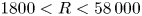 $1800< R<58\,000$. The growth of the type-II instability peaks at approximately
  $R=10^4$, where
  $-\alpha _i = 0.0098$. If the terms
  ${\mathcal {R}}_{x}$,
  ${\mathcal {R}}_{\varphi }$,
  ${\mathcal {C}}_{x}$ and
  ${\mathcal {C}}_{\varphi }$ are removed from (2.14b) and (2.14d), the growth rates of this mode, shown by the triangles, does not change apparently, especially when
  $R$ is high. The implication is that these terms play minor roles in driving the CM instability. However, when the terms
  ${\mathcal {R}}_{y}$ and
  ${\mathcal {C}}_{y}$ are removed from (2.14c), shown by the red dashed lines with triangles, the instability solutions only agree with the type-II branch in the limit of
  $R\to \infty$. Actually, this growth can also be predicted by the Rayleigh equation, shown by the blue crosses, indicating its inviscid nature for large
  $R$ values. Examining its vortex structure shown in panel (c), we confirm that this type-II instability for
  $R>10^6$ is a new branch of cross-flow instability due to its co-rotating feature. As mentioned before, the type-II CM instability in a rotating-cone boundary layer differs from the Görtler instability on a concave wall because the curvature reduces as
  $R$ increases, which explains the phenomenon that the type-II CM eventually transitions to the type-II CFM as
  $R\to \infty$.
It is more instructive to observe the variation of the vortex structures on  $R$. Figure 25(b) shows the stationary vortex structures of the type-I CFMs for different
  $R$. Because these modes are of the inviscid nature, as illustrated in figure 13, change of
  $R$ does not affect the co-rotating vortex structures apparently. The centre of the vortices is always located around the critical line. Panel (c) displays the vortex structure of the type-II instability. For
  $R=2000$, a pair of counter-rotating vortices in the interval
  $\alpha _{r}x+\beta r_{0} \varphi \in [0, 2{\rm \pi} )$ are observed, confirming the CM instability nature. Note that the asymmetric feature is in contrast to the Görtler vortices on a concave wall, because for the latter configuration, the effective velocity
  $\tilde U$ is zero everywhere. The counter-rotating vortices are marked by CWR (clockwise rotating) in the blue block and AWR (anti-clockwise rotating) in the black block. Increasing
  $R$ to
  $2 \times 10^4$, a new CWR vortex, also marked by a black block, appears in the near-wall region. For
  $R= 4 \times 10^4$, the lower CWR vortex moves further towards the wall. Further increasing
  $R$ to
  $1\times 10^7$, the lower CWR disappears, and the CWR and AWR vortices tend to be aligned in the vertical direction. Additionally, the centres of the two vortices are located at
  $y=1.76$ and 3.78, respectively, as marked by the horizontal dashed lines, agreeing with the positions of the two critical lines. Such a structure evolution clearly shows the transition from the type-II CM to the type-II CFM in the large-
 $R$ limit.
To this end, we are able to summarise the critical parameters for the onset of the type-I CFM and type-II CM instabilities for different  $\bar \varOmega$ values, as listed in table 2. As
  $\bar \varOmega$ increases,
  $R_c$ for both modes decreases monotonically, indicating a promotion of these instabilities by the rotating speed. For a fix
  $\bar \varOmega$, the wavelength of the type-II CM is shorter than that of the type-I CFM, which agrees with the perturbation structures in figure 18(b,c).
Table 2. Critical parameters for the onset of the stationary type-I CFM and the type-II CM instabilities, where  $R_c$,
  $\alpha _{r,c}$ and
  $\beta _c$ denote the critical Reynolds number, streamwise wavenumber and spanwise wavenumber, respectively.

5. Summary and conclusions
In this paper, the linear instability of a Mach 3 boundary layer over a  $7^\circ$-semi-apex-angle rotating cone with zero angle of attack is studied. Unlike the axisymmetric configuration, the base flow on a rotating cone does not admit a self-similarity solution, and a marching scheme starting from the cone tip is employed to solve the compressible BLEs. It is found that the boundary layer grows like
  $x^{1/2}$, similar to that of the axisymmetric configuration, but the boundary-layer thickness is slightly thinner. The velocity and temperature in the near-wall region become greater as the rotation rate increases. The accuracy of the boundary-layer solutions is confirmed by comparing with the full N-S solutions; see Appendix B.
Based on the base flow obtained by the compressible BLEs, a systematic instability analysis is performed, and different instability regimes appear in the  $R$–
$R$– $\bar \varOmega$ plane, as sketched in figure 26.

Figure 26. Different instability mechanisms in the  $R$–
$R$– $\bar \varOmega$ plane.
For a sufficiently small  $\bar \varOmega$ (
 $\bar \varOmega \ll 1$), only the type-I MMM instability occurs, which is found to be an extension of the Mack first mode in a 2-D boundary layer to the rotation configuration. In the long-wavelength (lower-branch) limit, the phase speed approaches the slow acoustic wave propagating along the potential-flow-streamline direction (
 $\tilde U_e-1/M$), whereas in the upper-branch limit, the phase speed approaches the effective velocity at the GIP (
 $\tilde U_c$). In the large-
 $R$ limit, the unstable MMM shows a double-deck structure (Dong et al. Reference Dong, Liu and Wu2020; Dong & Zhao Reference Dong and Zhao2021), as sketched in figure 27(a). In the main layer where
  $y=O(1)$, the instability to leading order is described by the Rayleigh equation. Because the Rayleigh solution does not satisfy the no-slip condition at the wall, a viscous Stokes layer where
  $y=O(R^{-1/2})$ appears in the near-wall region. At the lower and upper neutral points, however, the Rayleigh equation becomes singular at
  $\tilde U=\tilde U_e-1/M$ and
  $\tilde U=\tilde U_c$, respectively, and so a viscous critical layer with a thickness of
  $O(R^{-1/3})$ must be taken into account (Gajjar et al. Reference Gajjar, Arebi and Sibanda1996; Wu Reference Wu2019); see the asymptotic structure shown in figure 27(b). Due to the presence of the circumferential velocity, the MMM is not symmetric about the
  $\beta =0$ line. The effects of Coriolis force, centrifugal force and curvature only produce an almost negligible correction on the MMM instability.

Figure 27. Asymptotic structures of the inviscid mode: (a) in the unstable frequency or wavenumber band; (b) around the neutral point, with  $y_c$ denoting the location of the critical layer.
When  $\bar \varOmega$ is increased to a moderate level, say
  $\bar \varOmega =0.3$, a type-I CFM, connecting with the type-I MMM, appears in the vicinity of zero-frequency band, which is found to be driven by the cross-flow effect induced by the rotating velocity. Its oblique wave angle approaches
  $\varTheta _e$ (the direction perpendicular to the potential-flow streamline) in the upper-branch vicinity, but approaches
  $\varTheta _s$ (the direction perpendicular to the wall shear) in the lower-branch vicinity. The implication is that the two branches of CFM belong to different instability regimes. The majority of the CFM, including the most unstable and upper-branch quasi-neutral states, belong to the inviscid nature, which shows a double-deck structure as sketched by figure 27(a). Also, at the upper-branch neutral point, the critical layer appears, whose asymptotic structure is the same as that shown in figure 27(b). However, in the lower-branch vicinity, the CFM shows a viscous-inviscid interactive nature, whose asymptotic triple-deck structure is plotted in figure 28. This regime is the same as those reported by Malik (Reference Malik1986) and Hall (Reference Hall1986). A simple visualisation of the CFM vortices shows a co-rotating structure, agreeing with the CFM in other configurations, such as rotating-disc and swept-wing boundary layers (Kobayashi et al. Reference Kobayashi, Kohama and Takamadate1980; Kohama Reference Kohama1987; Kobayashi Reference Kobayashi1994).

Figure 28. Asymptotic structure of the viscous-inviscid-interactive (triple-deck) instability.
Further increase of  $\bar \varOmega$ to an
  $O(1)$ level, say
  $\bar \varOmega =0.75$, the centrifugal instability, referred to as the type-II CM instability, is found to coexist with the type-I modes, whose growth rate is comparable to the latter. At a moderate
  $R$, the type-II instability is driven by the centrifugal force, for which the flow field with a finite-amplitude CM show a counter-rotating vortex structure. Such a structure is also observed in other experiments, such as (Kobayashi et al. Reference Kobayashi, Kohama and Kurosawa1983; Kobayashi Reference Kobayashi1994). The type-II instability is enhanced as
  $\bar \varOmega$ increases. Following Hall (Reference Hall1982), we know that for asymptotically large
  $T_a$, the CM instability near the upper-branch neutral point is driven by the balance between the centrifugal effect and viscosity, which is confirmed by the energy analysis. Being different from the traditional Görtler instability appearing in a boundary layer over a concave wall, the type-II CM on a rotating cone cannot be sustained in the high-
 $R$ limit, because the centrifugal effect decreases with increase of
  $R$. When
  $R$ is increased to a sufficiently high level, the type-II CM morphs into the type-II CFM, which is driven by the cross-flow effect. The type-II CFM can coexist with the type-I CFM in a high
  $R$, but they are distinguished by their wavenumbers, growth rates and eigenfunctions. The main difference of their instability feature is caused by the difference of their effective velocities; a demonstration can be seen in figure 25(b). As
  $\bar \varOmega$ increases, the transitional Reynolds number from the type-II CM to the type-II CFM becomes higher.
It is noted that all the instabilities discussed above are of convective-instability nature, and the absolute instability, as discovered in rotating discs (Lingwood Reference Lingwood1995, Reference Lingwood1996) or the Taylor–Couette flow (Babcock, Ahlers & Cannell Reference Babcock, Ahlers and Cannell1991; Tsameret & Steinberg Reference Tsameret and Steinberg1994), is not observed for the present configuration. According to Garrett & Peake (Reference Garrett and Peake2007) and Garrett, Hussain & Stephen (Reference Garrett, Hussain and Stephen2010), as the axial flow increases and/or the semi-apex angle decreases, the critical Reynolds number of the absolute instability would increase remarkably. Thus, for the present configuration with a high-level axial flow and a small half-apex angle, the transition may be attributed dominantly to the accumulation of the convective instability, instead of the absolute instability.
The present study only focuses on a supersonic regime with  $M=3$. If the Mach number is increased to a hypersonic level, the Mack second mode with a greater growth rate would appear, and its development on the rotating cone would also be interesting, which will be probed in the future. We also note that in the present work, calculating the growth rate for different
  $R$ values with
  $X$ fixed is not equivalent to the evolution of an instability on the cone surface, and a more appropriate calculation should be conducted based on the parabolised stability equations, which is also considered to be our future work.
Funding
This work is supported by the National Science Foundation of China (Grant Nos U20B2003, 11988102) and Strategic Priority Research Program, CAS (No. XDB22040104).
Declaration of interests
The authors report no conflict of interest.
Appendix A. The non-zero element of the coefficient matrix  $\boldsymbol{\mathsf{A}}$

The dimension of the coefficient matrix  $\boldsymbol{\mathsf{A}}$ in (2.20) is 8
 $\times$8, and its non-zero elements are
 \begin{gather} {A_{14}} ={-} \frac{U_{B,y}{\mu _{B,T}}}{ \mu_B},\quad {A_{15}} = 1;\quad {A_{21}} \!=\!{-} \text{i} \alpha -\tan \theta \bar \kappa,\quad {A_{22}} \!=\! {\frac{{{\tilde Q T _{B,y}}}}{T_B } - \bar \kappa} ,\quad {A_{23}} \!=\!{-} \text{i} \tilde \beta, \end{gather}
 \begin{gather} {A_{24}} = \frac{{\tilde S \tilde Q}}{T_B},\quad {A_{26}} =\frac{\gamma M^2 \tilde S\tilde Q \mu_B }{R} ;\quad {A_{33}} = \bar \kappa, {A_{34}} ={-}( W_{B,y}- \bar \kappa W_B) \frac{{ \mu }_{B,T}}{\mu_B} ,\quad {A_{37}} = 1; \end{gather}
 \begin{gather} {A_{44}} ={-} \frac{{{ \mu }_{B,y}}}{\mu_B} ,\quad {A_{48}} = 1;\quad {A_{51}} = \frac{{R \tilde S T_B}}{{ \mu_B }} + \bar\alpha^2, \end{gather}
 \begin{gather} {A_{52}} = \frac{{R U_{B,y}}}{{ \mu_B T_B }} - \frac{l_2 \gamma M^2 \tilde Q T _{B,y}}{{T_B}^{2}} [\varOmega \sin \theta \left( {{{ \varOmega }} r + 2 W_B} \right) +\tan \theta \bar \kappa W_{B}^{2}] \nonumber\\ - \text{i} \alpha\left( \frac{{{{ \mu }_{B,y}}}}{{ \mu_B }} - {\frac{{{\tilde Q T _{B,y}}}}{T_B } } \right), \end{gather}
 \begin{gather} {A_{53}} = \frac{{ - 2 R (\varOmega \sin \theta+ \tan \theta \bar \kappa W_B) }}{{\mu_B T_B }},\quad {A_{54}} = \frac{{\text{i} \alpha\tilde Q \tilde S}}{T_B}\nonumber\\ \quad+ \frac{R \varOmega \sin \theta \tilde Q [\left( {{{ \varOmega }} r + 2 W_B} \right) +\tan \theta \bar \kappa W_{B}^{2}] }{{{T_B}^{2} \mu_B }}, \end{gather}
 \begin{gather} {A_{55}} ={-} \left( {\bar \kappa + \frac{{{{ \mu }_{B,y}}}}{{ \mu_B }}} \right),\quad {A_{56}} = \tilde Q \left [ \frac{\varOmega \sin \theta \left( {{{ \varOmega }} r + 2 W_B} \right)+\tan \theta \bar \kappa W_{B}^{2}}{T_B}\right.\nonumber\\ \left. \quad - \text{i} \alpha\left( {1 + l_1 \gamma M^2 \tilde S \mu_B } \right) \vphantom{\left [ \frac{\varOmega \sin \theta \left( {{{ \varOmega }} r + 2 W_B} \right)+\tan \theta \bar \kappa W_{B}^{2}}{T_B}\right.}\right]; \end{gather}
 \begin{gather} {A_{61}} = \frac{{{{2\text{i} \alpha \mu }_{B,y}}}}{{ \mu_B }}, \end{gather}
 \begin{gather} A_{62} = \frac{R \tilde S }{{ \mu_B T_B }} + { { \frac{2 \bar \kappa {{ \mu }_{B,y}}}{\mu_B}}} + \bar\alpha^2 - \frac{ l_2 \gamma M^2 \tilde Q T_{B,y}}{{T_B}^2} \left( { \bar \kappa {W_{B}^2} + 2 \varOmega \cos \theta W_B + {{ \varOmega }^2}\cos \theta r} \right), \end{gather}
 \begin{gather} {A_{63}} = 2\text{i} \tilde \beta \left( {\frac{{{{ \mu }_{B,y}}}}{{ \mu_B }} + \bar \kappa} \right) - \frac{2 R }{{ \mu_B T_B }}\left( {\bar \kappa W_B + \varOmega \cos \theta } \right), \end{gather}
 \begin{gather} {A_{64}} = \frac{R \tilde Q }{ \mu_B {T_B}^2 } \left( {\bar \kappa {W_{B}^2} +\! 2 \varOmega \cos \theta W_B + {{ \varOmega }^2}\cos \theta r} \right) -\! \frac{{{{2 \mu }_{B,T}}}}{{ \mu_B }}\left[ {\text{i} \alpha U_{B,y} +\! \text{i} \tilde \beta (W_{B,y}\!- \bar \kappa W_B) } \right], \end{gather}
 \begin{gather} {A_{65}} = \text{i} \alpha,\quad {A_{66}} = \frac{\tilde Q}{T_B} \left( {\bar \kappa {W_{B}^2} + 2 \varOmega \cos \theta W_B + {{ \varOmega }^2}\cos \theta r} \right) - \frac{{{{ \mu }_{B,y}}}}{{ \mu_B }},\quad {A_{67}} = \text{i} \tilde \beta; \end{gather}
 \begin{gather} {A_{71}} = \frac{{ R [2\varOmega \sin \theta +\tan \theta W_B ( \kappa + \bar \kappa) ] }}{{ \mu_B T_B }}, \end{gather}
 \begin{gather} {A_{72}} = \frac{R }{{ \mu_B T_B }}\left( {2 \varOmega \cos \theta + W_{B,y}+ \bar \kappa W_B} \right) - \text{i} \tilde \beta \left( {2 \bar \kappa + \frac{{{{ \mu }_{B,y}}}}{{ \mu_B }} - \frac{{{ \tilde Q T _{B,y} }}}{T_B }} \right) \nonumber\\ + \frac{l_2 \gamma M^2 \tilde Q T_{B,y} U_B[2 \varOmega \sin \theta +\tan \theta W_B ( \kappa + \bar \kappa)] }{{T_B}^2} , \end{gather}
 \begin{gather} {A_{73}} = \frac{{R (\tilde S+ \tan \theta \bar \kappa U_B) }}{{ \mu_B T_B}} +\bar\alpha^2,\quad {A_{74}} ={-} \frac{ R \tilde Q U_B [2 \varOmega \sin \theta +\tan \theta W_B ( \kappa + \bar \kappa)]}{ \mu_B {T_B}^{2} } + \frac{{\text{i} \tilde \beta \tilde Q\tilde S}}{T_B}, \end{gather}
 \begin{gather} {A_{76}} = \frac{\gamma M^2 \tilde Q U_B [2 \varOmega \sin \theta +\tan \theta W_B ( \kappa + \bar \kappa)] }{T_B}\nonumber\\ \quad - \text{i} \tilde \beta \tilde Q\left( {1 + l_1 \gamma M^2 \tilde S \mu_B } \right),\quad {A_{77}} ={-} \left( {2 \bar \kappa + \frac{{{{\tilde \mu }_{B,y}}}}{{\tilde \mu_B }}} \right); \end{gather}
 \begin{gather} {A_{82}} ={-} \left( {\gamma - 1} \right)M^2 Pr {\left[ {\text{i} \alpha U_{B,y} + \text{i} \tilde \beta (W_{B,y}- \bar \kappa W_B) } - \frac{{R \tilde Q{T _{B,y}}}}{{ \gamma M^2 \mu_B T_B }} \right] } + \frac{Pr {\kern 1pt} R {T_{B,y}}}{{\gamma \mu_B T_B }} , \end{gather}
 \begin{gather} {A_{84}} = \left( {\gamma - 1} \right)M^2 Pr \left\{ {\left[ {U_{B,y}^2 + (W_{B,y}-\bar \kappa W_B )^2} \right]\frac{{{{ \mu }_{B,T}}}}{{ \mu_B }} + \frac{{R \tilde S\tilde Q }}{{\gamma M^2 \mu_B {T_B}^{2}}}} \right\} +\frac{{Pr{\kern 1pt} R \tilde S }}{{\gamma \mu_B T_B }} + \bar\alpha^2, \end{gather}
 \begin{gather} {A_{85}} ={-} 2 \left( {\gamma - 1} \right)M^2 Pr U_{B,y},\quad {A_{86}} = \left( {\gamma - 1} \right)M^2 Pr \tilde S \tilde Q, \end{gather}
 \begin{gather} {A_{87}} ={-} 2 \left( {\gamma - 1} \right)M^2 Pr( W_{B,y}- \bar \kappa W_B),\quad {A_{88}} ={-} \frac{{{{ \mu }_{B,y}}}}{{ \mu_B }} - \bar \kappa ; \end{gather}
where  $\bar \alpha =\sqrt { \alpha ^2 + \tilde \beta ^2}$,
  $\tilde Q = {[ {1 + {4 \gamma M^2 \mu _B \tilde S}/{(3 R)} } ]^{ - 1}}$, and
  $l_j = j - 2/3 (j=1,2)$.
Appendix B. Verification of the base-flow calculations
To confirm the accuracy of the solutions of the compressible BLEs (2.10), we also carry out calculations by solving the full N-S equations (2.1). In the numerical process, the N-S equations (2.1) are re-expressed in terms of the conservative form, and the nonlinear convective and viscous terms are discretised by the second-order total-variation-diminishing (TVD) scheme and the second-order central scheme, respectively. The implicit lower-upper symmetric Gauss–Seidel (LU-SGS) method is employed for the time advancing. The 3-D calculation is based on the Cartesian coordinate system,  $(\bar x,\bar y,\bar z)=(x\cos \theta -y\sin \theta, (x \sin \theta + y \cos \theta )\cos \varphi, (x \sin \theta + y \cos \theta ) \sin \varphi )$, and the computational domain for the
  $\bar z=0$ plane, is demonstrated in figure 29. To avoid the singularity at the nose tip, we introduce a small bluntness with a radius of
  $r_0=0.05$, as shown in the inset. According to Sivasubramanian & Fasel (Reference Sivasubramanian and Fasel2015), the effect of the bluntness is confirmed to be negligible when
  $x$ is over 2000
 $r_0$, and in our case, we have chosen
  $x\approx 40\,000r_0$. The number of the grid points is chosen to be
  $801\times 301\times 201$, for which careful resolution tests have been performed. The inflow is set to be the supersonic oncoming stream. From the inviscid conic-flow theory (Sims Reference Sims1964), we can estimate the oncoming Mach number and temperature of the supersonic stream to be
  $M_\infty =3.214$ and
  $T_\infty =48.28K$, respectively. It is then calculated that the unit Reynolds number is
  $9.26 \times 10^6$. The no-slip and isothermal conditions are applied at the wall, while the extrapolated condition is applied at the outflow boundary. The contours of the mean pressure
  $\bar p$ are also shown in figure 29, in which the location of the oblique shock is clearly observed.

Figure 29. Sketch of the computation domain and the contours of the mean pressure.
Figure 30 compares the wall-normal profiles of  $U_B$,
  $W_B$ and
  $T_B$ at
  $X=1$ obtained by the full N-S equations (2.1) and compressible BLEs (2.10). Good agreement is achieved, confirming the accuracy of our BLE solutions.

Figure 30. Comparisons of the base-flow profiles obtained by solving the boundary-layer and the N-S equations at  $X=1$ for
  $\bar \varOmega =0.3$.
Appendix C. The lower-branch CFM: asymptotic analysis and numerical results
C.1. Asymptotic analysis I: Coriolis-force-induced instability
The lower-branch CFM shows a viscous-inviscid interactive nature, described by the triple-deck structure as in figure 28. A scaling derivation is as follows. In the main deck where  $y=O(1)$, only the inertia terms remain in the leading-order balance. Following Hall (Reference Hall1986), Choudhari (Reference Choudhari1995), Liu, Dong & Wu (Reference Liu, Dong and Wu2020) and Dong & Zhao (Reference Dong and Zhao2021), we know that the perturbation field to leading order behaves like
 \begin{equation} \hat u=\hat AU_{B,y},\quad\hat v={-}{\rm i}(\alpha U_B+\beta W_B)\hat A\quad \hat w=\hat AW_{B,y},\quad\hat T=\hat A T_{B,y}, \end{equation}
where  $\hat A$ is the displacement function characterising the instability amplitude.
Apparently, as  $y\rightarrow \infty$, the perturbation
  $\hat v=O(\alpha \hat A)$ does not vanish, failing to satisfy the attenuation condition in the far field. This requires us to take into account an upper deck where
  $y\sim \alpha ^{-1}$. Note that the lower-branch CFM shows a long-wavelength nature, for which
  $\alpha \ll 1$. In this layer,
  $\hat p$,
  $\hat u$ and
  $\hat v$ are of the same order of magnitude. Matching with the main layer, we obtain
 \begin{equation} \hat p\sim\hat v=O(\alpha\hat A). \end{equation}
 Applying (C1a,c,d) at  $y=0$, we find that the no-slip, isothermal conditions are not satisfied, which requires the introduction of the lower deck in the near-wall region. In this layer, the inertia term balances the viscous term,
  $\tilde \alpha \tilde U \hat {u} \sim R^{-1} \hat {u}_{yy}$. Since the wave vector is perpendicular to the wall shear direction, we can approximate
  $\tilde U$ by
  $\bar C y^{2}$ in the near-wall region, where
  $\bar C$ is a constant. Thus, the thickness of the lower deck is estimated as
 \begin{equation} y \sim (\tilde \alpha R)^{- {1}/{4}}\sim ( \alpha R)^{- {1}/{4}}. \end{equation}
Note that for this CFM, because the wave angle is neither 0 $^\circ$ nor 90
 $^\circ$, we know that
  $\alpha \sim \beta$ and so
  $\alpha \sim \tilde \alpha =\sqrt {\alpha ^2+\beta ^2}$. The pressure gradient
  $\textrm {i} \alpha \hat {p}$ does not appear in the leading-order balance, but it balances the Coriolis-force term,
  $2 \varOmega \sin \theta \rho _B \hat {w}$. Since
  $\varOmega \sim R^{-1}$, we obtain
 \begin{equation} \hat{p} \sim (\alpha R)^{{-}1} \hat{w}\sim(\alpha R)^{{-}1}\hat A, \end{equation}
where  $\hat w\sim \hat A$ is obtained by applying (C1c) at the wall. Combining (C4) with (C2), we can estimate that
 \begin{equation} \alpha \sim R^{-{1}/{2}}. \end{equation}
This scaling was also found by Hall (Reference Hall1986) in the CFM for an incompressible rotating-disc boundary layer. The compressibility for this mode does not affect the asymptotic scaling at all. Thus, from (C3), we know that the lower-deck thickness is  $O(R^{-{1}/{8}})$.
C.2. Asymptotic analysis II: wall-shear-induced instability
It is noted that the Coriolis force is proportional to  $\varOmega \sin \theta$, and for a small apex angle,
  $\sin \theta$ is numerically small. Therefore, if
  $\varOmega$ is also small, the aforementioned regime, showing a scaling law (C5), might be overwhelmed by another regime. In the study of the CFM in a swept boundary layer without the Coriolis effect (Butler & Wu Reference Butler and Wu2018), it was pointed out that a long-wavelength triple-deck deck regime appears, in which non-parallelism has a leading-order effect on the growth rate. Actually, such a regime was also reported by Choudhari (Reference Choudhari1995) even when the non-parallelism is absent. The key factor to this regime is the appearance of the high-order expansion of the base-flow profile.
In the near-wall region, the effective velocity  $\tilde U$ introduced in (4.2) can be expanded in terms of a Maclaurin series,
  $\tilde U=\sum _{n=1}^\infty c_n y^n$. Since the base-flow velocity is perpendicular to the wave angle of the CFM, we obtain that
  $c_1=0$. Following Butler & Wu (Reference Butler and Wu2018), we know that the pressure gradient
  $\textrm {i}\alpha \hat p$ does not appear in the lowest-order balance, where the inertia term
  $\sim \textrm {i}\alpha c_2 y^2\hat u$. Similarly, the pressure gradient is also not possible to balance the second-lowest-order inertia term. For the third order, the balance
  $\alpha ^2\sim \alpha (\alpha R)^{-1}$ leads to
  $\alpha \sim R^{-1/2}$, the scaling law for the Coriolis-force-induced instability (C5). This indicates that the inertia term
  $\textrm {i}\alpha c_4y^4\hat u$ appears also in the balance induced by the Coriolis force discussed in § C.1.
If the rotating rate is sufficiently small, for which the Coriolis force is rather weak, the pressure-gradient term  $\textrm {i}\alpha \hat p$ is possible to balance with the inertia term at the next order,
  $\textrm {i}\tilde \alpha c_5y^5\hat u$, which, combining with (C2) and (C3), leads to
  $\alpha ^2\sim \alpha (\alpha R)^{-5/4}$, i.e.
 \begin{equation} \alpha\sim R^{{-}5/9}. \end{equation}
This scaling law is the same as that of Butler & Wu (Reference Butler and Wu2018). For the cases considered in the present paper, this regime is likely to appear when  $\varOmega$ is rather small.
Actually, changing the rotating rate  $\varOmega$ leads to a variation of the base-flow profiles, so does the coefficient
  $c_n$ in the Maclaurin expansion. If, for some specific case,
  $c_5$ is numerically small, then the pressure gradient could balance with an even higher-order inertia term. It is not difficult to conclude that the balance between the inertia term
  $\textrm {i}\alpha c_n y^n \hat u$ and the pressure gradient lead to a generic form of the scaling law,
 \begin{equation} \alpha\sim R^{{-}n/n+4},\quad n\geq 4. \end{equation}
This set of scaling laws are all possible for an instability based on the parallel-flow assumption. Particularly, if we take  $n=8$, the scaling law
  $\alpha \sim R^{-2/3}$ as in figure 12(b) is recovered.
C.3. Numerical results
The scaling law of  $\alpha \sim R^{-1/2}$ as in § C.1 is not the same as that observed in figure 12(b), where
  $\alpha \sim \tilde \alpha \sim R^{-2/3}$, which needs to be explained in this subsection.
To show the impact of the rotating rate on the lower-branch neutral curve, figure 31(a) plots the dependence of its effective wavenumber  $\tilde \alpha$ on
  $R$ with
  $\bar \varOmega$ increasing from 0.1 to 1.5. For
  $\bar \varOmega \leq 0.5$,
  $\tilde \alpha$ decreases with
  $R$ monotonically, but the decay rates increase with
  $\bar \varOmega$ slightly. When
  $\bar \varOmega$ is increased to 0.75, the decay rate changes remarkably when
  $R>2\times 10^6$. Further increase of
  $\bar \varOmega$ leads to an upstream movement of the onset of this rapid change. When
  $\bar \varOmega$ reaches 1.25 and 1.5, the decay rate of
  $\tilde \alpha$ with respect to
  $R$ shows agreement with the asymptotic prediction (C5). Thus, the whole picture is clear. The scaling law (C5) is indeed an ultimate regime when
  $R$ is sufficiently large; before reaching this scaling, there could exist other scaling laws for smaller Reynolds numbers. The appearance of this ultimate scaling law is earlier when the rotating rate is increased. It is also predicted that, for
  $\bar \varOmega =0.3$, the ultimate regime will be reached when
  $R$ is greater than
  $2\times 10^7$, which is however difficult to be verified because the Reynolds number is required to be an extremely high value. Additionally, we note that the Coriolis force scales with
  $\varOmega \sin \theta$, which is numerically small especially when the rotating rate is low. Thus, the instability may be driven by the high-order wall shear, instead of the Coriolis force, and the scaling law (C6) is approximately arrived for
  $\bar \varOmega =0.1$, as confirmed by the circles in figure 31. Non-parallelism will need to be studied as it has a leading-order effect on the growth rate and hence on the precise neutral curve (Butler & Wu Reference Butler and Wu2018).

Figure 31. Variation with  $R$ of the lower-branch neutral curve of the type-I CFM for different
  $\bar \varOmega$ at
  $X=1$.


