


1. Introduction
Advancing our conceptual understanding and ability to predictively model exchange processes between urban areas and the atmosphere is of critical importance to a wide range of applications, including urban air quality control (Britter & Hanna Reference Britter and Hanna2003; Barlow, Harman & Belcher Reference Barlow, Harman and Belcher2004; Pascheke, Barlow & Robins Reference Pascheke, Barlow and Robins2008), urban microclimate studies (Roth Reference Roth2012; Li & Bou-Zeid Reference Li and Bou-Zeid2014; Ramamurthy, Li & Bou-Zeid Reference Ramamurthy, Li and Bou-Zeid2017) and weather and climate forecasting (Holtslag et al. Reference Holtslag2013), to name but a few. It hence comes as no surprise that substantial efforts have been devoted towards this goal over the past decades, via, e.g. numerical simulations (Bou-Zeid, Meneveau & Parlange Reference Bou-Zeid, Meneveau and Parlange2004; Xie, Coceal & Castro Reference Xie, Coceal and Castro2008; Cheng & Porté-Agel Reference Cheng and Porté-Agel2015; Giometto et al. Reference Giometto, Christen, Meneveau, Fang, Krafczyk and Parlange2016; Auvinen et al. Reference Auvinen, Järvi, Hellsten, Rannik and Vesala2017; Sadique et al. Reference Sadique, Yang, Meneveau and Mittal2017; Zhu et al. Reference Zhu, Iungo, Leonardi and Anderson2017; Li & Bou-Zeid Reference Li and Bou-Zeid2019), wind tunnel experiments (Raupach, Thom & Edwards Reference Raupach, Thom and Edwards1980; Böhm et al. Reference Böhm, Finnigan, Raupach and Hughes2013; Marucci & Carpentieri Reference Marucci and Carpentieri2020) and observational studies (Rotach Reference Rotach1993; Kastner-Klein & Rotach Reference Kastner-Klein and Rotach2004; Rotach et al. Reference Rotach2005; Christen, Rotach & Vogt Reference Christen, Rotach and Vogt2009). These studies have explored the functional dependence of flow statistics on urban canopy geometry (Lettau Reference Lettau1969; Raupach Reference Raupach1992; Macdonald, Griffiths & Hall Reference Macdonald, Griffiths and Hall1998; Coceal & Belcher Reference Coceal and Belcher2004; Yang et al. Reference Yang, Sadique, Mittal and Meneveau2016; Li & Katul Reference Li and Katul2022), characterized the topology of coherent structures (Kanda, Moriwaki & Kasamatsu Reference Kanda, Moriwaki and Kasamatsu2004; Christen, van Gorsel & Vogt Reference Christen, van Gorsel and Vogt2007; Coceal et al. Reference Coceal, Dobre, Thomas and Belcher2007; Li & Bou-Zeid Reference Li and Bou-Zeid2011; Inagaki et al. Reference Inagaki, Castillo, Yamashita, Kanda and Takimoto2012) and derived scaling laws for scalar transfer between the urban canopy and the atmosphere (Pascheke et al. Reference Pascheke, Barlow and Robins2008; Cheng & Porté-Agel Reference Cheng and Porté-Agel2016; Li & Bou-Zeid Reference Li and Bou-Zeid2019), amongst others. Most of the previous works have focused on atmospheric boundary layer (ABL) flow under (quasi) stationary conditions. However, stationarity is a rare occurrence in the ABL (Mahrt & Bou-Zeid Reference Mahrt and Bou-Zeid2020), and theories based on equilibrium turbulence are, therefore, often unable to grasp the full range of physics characterizing ABL flow environments.
Major drivers of non-stationarity in the ABL include time-varying horizontal pressure gradients, associated with non-turbulent motions ranging from submeso to synoptic scales, and time-dependent thermal forcings, induced by the diurnal cycle or by cloud-induced time variations of the incoming solar radiation (Mahrt & Bou-Zeid Reference Mahrt and Bou-Zeid2020). These conditions often result in departures from equilibrium turbulence, with important implications on time- and area-averaged exchange processes between the land surface and the atmosphere. The first kind of non-stationarity was examined in Mahrt (Reference Mahrt2007, Reference Mahrt2008) and Mahrt et al. (Reference Mahrt, Thomas, Richardson, Seaman, Stauffer and Zeeman2013), which showed that time-variations of the driving pressure gradient could enhance momentum transport under strong stable atmospheric stratifications. The second kind of non-stationarity was instead analysed in Hicks et al. (Reference Hicks, Pendergrass, Baker, Saylor, O'Dell, Eash and McQueen2018), making use of data from different field campaigns, and showed that the surface heat flux could change so rapidly during the morning and late afternoon transition that the relations for equilibrium turbulence no longer hold.
Numerical studies have also been recently conducted to study how exchange processes between the land surface and the atmosphere are modulated by non-stationarity in the ABL. In their study, Edwards Edwards, Beare & Lapworth (Reference Edwards, Beare and Lapworth2006) conducted a comparison of a prevailing single-column model based on equilibrium turbulence theories with the observations of an evening transition ABL, as well as results from large-eddy simulations (LES). Their findings emphasized the inadequacy of equilibrium turbulence theories in capturing the complex behaviour of ABL flows during rapid changes in thermal surface forcing. This breakdown of equilibrium turbulence was particularly notable during the evening transition period, which is known for its rapid changes in thermal forcing. Momen & Bou-Zeid (Reference Momen and Bou-Zeid2017) investigated the response of the Ekman boundary layer to oscillating pressure gradients, and found that quasiequilibrium turbulence is maintained only when the oscillation period is much larger than the characteristic time scale of the turbulence. The majority of the efforts have focused on ABL flow over modelled roughness, where the flow dynamics in the roughness sublayer – that layer of the atmosphere that extends from the ground surface up to approximately 2–5 times the mean height of roughness elements (Fernando Reference Fernando2010) – are bypassed, and surface drag is usually evaluated via an equilibrium wall-layer model (see, e.g. Momen & Bou-Zeid Reference Momen and Bou-Zeid2017), irrespective of the equilibrium-theory limitations outlined above. It hence remains unclear how unsteadiness impacts flow statistics and the structure of atmospheric turbulence in the roughness sublayer. Roughness sublayer flow directly controls exchanges of mass, energy and momentum between the land surface and the atmosphere, and understanding the dependence of flow statistics and structural changes in the turbulence topology on flow unsteadiness is therefore important in order to advance our ability to understand and predictively model these flow processes.
This study contributes to addressing this knowledge gap by focusing on non-stationarity roughness sublayer flow induced by time-varying pressure gradients. Unsteady pressure gradients in the real-world ABL can be characterized by periodic and aperiodic variations in both magnitude and direction. In this study, we limit our attention to a pulsatile streamwise pressure-gradient forcing, consisting of a constant mean and a sinusoidal oscillating component. This approach has two major merits. First, the temporal evolution of flow dynamics and associated statistics, as well as structural changes in turbulence, can be easily characterized thanks to the time-periodic nature of the flow unsteadiness. Second, the time scale of the pulsatile forcing is well defined, and can hence be varied programmatically to encompass a range of representative flow regimes.
Pulsatile turbulent flows over aerodynamically smooth surfaces have been the subject of active research in the mechanical engineering community because of their relevance across a range of applications; these include industrial (e.g. a rotating or poppet valve) and biological (blood in arteries) flows. The corresponding laminar solution is an extension of Stokes's second problem (Stokes Reference Stokes1901), where the modulation of the flow field by an unsteady pressure gradient is confined to a layer of finite thickness known as the ‘Stokes layer’. The thickness of the Stokes layer  $\delta _s$ is a function of the pulsatile forcing frequency $\omega$, i.e. $\delta _s=2l_s$, where $l_s=\sqrt {2\nu /\omega }$ is the so-called Stokes length scale and $\nu$ is the kinematic viscosity of the fluid. In the turbulent flow regime, it has been found that the characteristics of the pulsatile flow are not only dependent on the forcing frequency, but also on the amplitude of the oscillation. Substantial efforts have been devoted to investigating this problem, from both an experimental (Ramaprian & Tu Reference Ramaprian and Tu1980, Reference Ramaprian and Tu1983; Tu & Ramaprian Reference Tu and Ramaprian1983; Mao & Hanratty Reference Mao and Hanratty1986; Brereton, Reynolds & Jayaraman Reference Brereton, Reynolds and Jayaraman1990; Tardu & Binder Reference Tardu and Binder1993; Tardu Reference Tardu2005) and a computational perspective (Scotti & Piomelli Reference Scotti and Piomelli2001; Manna, Vacca & Verzicco Reference Manna, Vacca and Verzicco2012, Reference Manna, Vacca and Verzicco2015; Weng, Boij & Hanifi Reference Weng, Boij and Hanifi2016). Scotti & Piomelli (Reference Scotti and Piomelli2001) drew an analogy to the Stokes length and proposed a turbulent Stokes length scale, which can be expressed in inner units as
 \begin{equation} l_t^+=\frac{u_\tau}{\nu}\left( \frac{2(\nu+\nu_t)}{\omega}\right)^{1/2}, \end{equation}
where  $u_\tau$ is the friction velocity based on the surface friction averaged over pulsatile cycles and $\nu _t$ is the so-called eddy viscosity. Parameterizing the eddy viscosity in terms of the Stokes turbulent length scale, i.e. $\nu _t = \kappa u_\tau l_t$, where $\kappa$ is the von Kármán constant, and substituting into (1.1) one obtains
 \begin{equation} l_t^+= l_s^+\left(\frac{\kappa l_s^+}{2}+\left(1+\left( \frac{\kappa l_s^+}{2}\right)^{{1}/{2}}\right) \right). \end{equation}
 When  $l_t^+$ is large (e.g. when $\omega \rightarrow 0$), the flow is in a quasisteady state. Under such a condition, the flow at each pulsatile phase resembles a statistically stationary boundary layer flow, provided that the instantaneous friction velocity is used to normalize statistics. As $\omega$ increases and $l_t^+$ becomes of the order of the open channel height $L_3^+$, the entire flow is affected by the pulsation, i.e. time lags occur between flow statistics at different elevations, and turbulence undergoes substantial structural changes from its equilibrium configuration. When $l_t^+< L_3^+/2$, the flow modulation induced by the pulsation is confined within the Stokes layer $\delta _s^+=2l_t^+$. Above the Stokes layer, one can observe a plug-flow region, with the turbulence being frozen to its equilibrium configuration and simply advected by the mean flow pulsation. A few years later, Bhaganagar (Reference Bhaganagar2008) conducted a series of direct numerical simulations (DNS) of low-Reynolds-number pulsatile flow over transitionally rough surfaces. She found that flow responses to pulsatile forcing are generally similar to those in smooth-wall cases, when the roughness size is of the same order of magnitude as the viscous sublayer thickness. The only exception is that, as the pulsation frequency approaches the frequency of vortex shedding from the roughness elements, the longtime averaged velocity profile deviates significantly from that of the steady flow case due to the resonance between the pulsation and the vortex shedding. In the context of a similar flow system, Patil & Fringer (Reference Patil and Fringer2022) also reported a comparable observation in their DNS study.
In addition to the work of Bhaganagar (Reference Bhaganagar2008) and Patil & Fringer (Reference Patil and Fringer2022), pulsatile flow over small-scale roughness, e.g. sand grain roughness, has also been studied extensively in the oceanic context, i.e. combined current-wave boundary layers, which play a crucial role in controlling sediment transport and associated erosion in coastal environments (Grant & Madsen Reference Grant and Madsen1979; Kemp & Simons Reference Kemp and Simons1982; Myrhaug & Slaattelid Reference Myrhaug and Slaattelid1989; Sleath Reference Sleath1991; Soulsby et al. Reference Soulsby, Hamm, Klopman, Myrhaug, Simons and Thomas1993; Mathisen & Madsen Reference Mathisen and Madsen1996; Fredsøe, Andersen & Sumer Reference Fredsøe, Andersen and Sumer1999; Yang et al. Reference Yang, Tan, Lim and Zhang2006; Yuan & Madsen Reference Yuan and Madsen2015). The thickness of the wave boundary layer, which is the equivalent of the Stokes layer in the engineering community, is defined as
 \begin{equation} \delta_w=\frac{2\kappa u_{\tau,max}}{\omega}, \end{equation}
where  $u_{\tau,max}=\sqrt {\tau _{max}}$, and $\tau _{max}$ denotes the maximum of kinematic shear stress at the surface during the pulsatile cycle. Within the wave boundary layer, mean flow and turbulence are controlled by the nonlinear interaction between currents and waves. Above this region, the modulation of turbulence by waves vanishes. The wall-normal distribution of the averaged velocity over the pulsatile cycle deviates from the classic logarithmic profile, and is characterized by a ‘two-log’ profile, i.e. the velocity exhibits a logarithmic profile with the actual roughness length within the wave boundary layer and a different one characterized by a larger roughness length further aloft (Grant & Madsen Reference Grant and Madsen1986; Fredsøe et al. Reference Fredsøe, Andersen and Sumer1999; Yang et al. Reference Yang, Tan, Lim and Zhang2006; Yuan & Madsen Reference Yuan and Madsen2015). Such behaviour was first predicted by a two-layer time-invariant eddy viscosity model by Grant & Madsen (Reference Grant and Madsen1979), followed by many variants and improvements (Myrhaug & Slaattelid Reference Myrhaug and Slaattelid1989; Sleath Reference Sleath1991; Yuan & Madsen Reference Yuan and Madsen2015).
On the contrary, pulsatile flow at high Reynolds numbers over large roughness elements, such as buildings, has received far less attention. Yu, Rosman & Hench (Reference Yu, Rosman and Hench2022) conducted a series of LES of combined wave-current flows over arrays of hemispheres, which can be seen as a surrogate of reefs near the coastal ocean. They focused only on low Keulegan–Carpenter numbers  $KC\sim O(1\unicode{x2013}10)$, where $KC$ is defined as the ratio between the wave excursion $U_w T$ and the diameter of the hemispheres, and $U_w$ and $T$ are the wave orbital velocity and the wave period, respectively (Keulegan et al. Reference Keulegan and Carpenter1958). However, conclusions from Yu et al. (Reference Yu, Rosman and Hench2022) cannot be readily applied to pulsatile flow over urban-like roughness (i.e. large obstacles with sharp edges), mainly because different surface morphologies yield distinct air–canopy interaction regimes under pulsatile forcings (Carr & Plesniak Reference Carr and Plesniak2017).
Motivated by this knowledge gap, this study proposes a detailed analysis on the dynamics of the mean flow and turbulence in high-Reynolds-number pulsatile flow over idealized urban canopies. The analysis is carried out based on a series of LES of pulsatile flow past an array of surface-mounted cuboids, where the frequency and amplitude of the pressure gradient are programmatically varied. The LES technique has been shown to be capable of capturing the major flow features of pulsatile flow over various surface conditions (Scotti & Piomelli Reference Scotti and Piomelli2001; Chang & Scotti Reference Chang and Scotti2004). The objective of this study is to answer fundamental questions pertaining to the impacts of the considered flow unsteadiness on the mean flow and turbulence in the urban boundary layer:
(i) Does the presence of flow unsteadiness alter the mean flow profile in a longtime-averaged sense? If so, how do such modifications reflect in the aerodynamic surface parameters?
(ii) To what extent does the unsteady pressure gradient impact the overall momentum transport and turbulence generation in a longtime-averaged sense within and above the canopy?
(iii) How do the phase-averaged mean flow and turbulence behave in response to the periodically varying pressure gradient? How are such phase-dependent behaviours controlled by the oscillation amplitude and the forcing frequency?
This paper is organized as follows. Section 2 introduces the numerical algorithm and the set-up of simulations, along with the flow decomposition and averaging procedure. Results are presented and discussed in § 3. Concluding remarks are given in § 4.
2. Methodology
2.1. Numerical procedure
A suite of LES is performed using an extensively validated in-house code (Albertson & Parlange Reference Albertson and Parlange1999a,Reference Albertson and Parlangeb; Bou-Zeid, Meneveau & Parlange Reference Bou-Zeid, Meneveau and Parlange2005; Chamecki, Meneveau & Parlange Reference Chamecki, Meneveau and Parlange2009; Anderson, Li & Bou-Zeid Reference Anderson, Li and Bou-Zeid2015; Fang & Porté-Agel Reference Fang and Porté-Agel2015; Giometto et al. Reference Giometto, Christen, Meneveau, Fang, Krafczyk and Parlange2016; Li et al. Reference Li, Bou-Zeid, Anderson, Grimmond and Hultmark2016). The code solves the filtered continuity and momentum transport equations in a Cartesian reference system, which read
 \begin{gather} \frac{\partial u_i}{\partial x_i}=0, \end{gather}
 \begin{gather} \frac{\partial u_i}{\partial t} + u_j \left(\frac{\partial u_i}{\partial x_j}-\frac{\partial u_j}{\partial x_i}\right) ={-} \frac{1}{\rho} \frac{\partial p^*}{ \partial x_i} - \frac{\partial \textsf{$\mathit{\tau}$}_{ij}}{\partial x_j} - \frac{1}{\rho }\frac{\partial p_\infty}{ \partial x_1} \delta_{i1}+F_i , \end{gather}
where  $u_1$, $u_2$ and $u_3$ are the filtered velocities along the streamwise $(x_1)$, cross-stream $(x_2)$ and wall-normal $(x_3)$ direction, respectively. The advection term is written in the rotational form to ensure kinetic energy conservation in the discrete sense (Orszag & Pao Reference Orszag and Pao1975). Here $\rho$ represents the constant fluid density, $\textsf{$\mathit{\tau}$} _{ij}$ is the deviatoric component of the subgrid-scale (SGS) stress tensor, which is evaluated via the scale-dependent dynamic (LASD) Smagorinsky model (Bou-Zeid et al. Reference Bou-Zeid, Meneveau and Parlange2005). The LASD model has been extensively validated in wall-modelled simulations of unsteady ABL flow (Momen & Bou-Zeid Reference Momen and Bou-Zeid2017; Salesky, Chamecki & Bou-Zeid Reference Salesky, Chamecki and Bou-Zeid2017) and in the simulation of flow over surface-resolved urban-like canopies (Anderson et al. Reference Anderson, Li and Bou-Zeid2015; Giometto et al. Reference Giometto, Christen, Meneveau, Fang, Krafczyk and Parlange2016; Li et al. Reference Li, Bou-Zeid, Anderson, Grimmond and Hultmark2016; Yang Reference Yang2016). Note that viscous stresses are neglected in the current study; this assumption is valid as the typical Reynolds number of the ABL flows is $Re\sim O(10^9)$, and the flow is in the fully rough regime. Here $p^*=p+\tfrac {1}{3}\rho \textsf{$\mathit{\tau}$} _{ii}+\tfrac {1}{2} \rho u_i u_i$ is the modified pressure, which accounts for the trace of SGS stress and resolved turbulent kinetic energy. The flow is driven by a spatially uniform but temporally periodic pressure gradient, i.e.
 \begin{equation} - {\partial p_\infty}/{\partial x_1} = \rho f_m\left[1+\alpha_p \sin(\omega t)\right] , \end{equation}
where  $f_m$ denotes the mean pressure gradient. Here $\alpha _p$ is a constant controlling the amplitude of the forcing, $\omega$ represents the forcing frequency and $\delta _{ij}$ is the Kronecker delta tensor.
Periodic boundary conditions apply in the wall-parallel directions, and free-slip boundary conditions are employed at the upper boundary. The lower surface is representative of an array of uniformly distributed cuboids, which serves as a surrogate of urban landscapes. This approach has been commonly adopted in fundamental studies of ABL processes due to its limited number of characteristic length scales, which makes it amenable to comprehensive examination and analytical treatment (Reynolds & Castro Reference Reynolds and Castro2008; Cheng & Porté-Agel Reference Cheng and Porté-Agel2015; Tomas, Pourquie & Jonker Reference Tomas, Pourquie and Jonker2016; Basley, Perret & Mathis Reference Basley, Perret and Mathis2019; Omidvar et al. Reference Omidvar, Bou-Zeid, Li, Mellado and Klein2020). Such an approach is justified on the basis that one should first study a problem in its simplest set-up before introducing additional complexities. Nonetheless, it is important to acknowledge that the introduction of randomness in roughness alters the flow characteristics and the generation of turbulence in rough-wall boundary layer flows. For example, Xie et al. (Reference Xie, Coceal and Castro2008) studied flows over random urban-like obstacles and found that turbulence features in the roughness sublayer are controlled by the randomness in the roughness. Giometto et al. (Reference Giometto, Christen, Meneveau, Fang, Krafczyk and Parlange2016) conducted an LES study and highlighted that roughness randomness enhances the dispersive stress in the roughness sublayer. Chau & Bhaganagar (Reference Chau and Bhaganagar2012) carried out a series of DNS of flow over transitionally rough surfaces, demonstrating that different levels of roughness randomness lead to distinct turbulence structures in the near-wall region and subsequently affect turbulence intensities.
Spatial derivatives in the wall-parallel directions are computed via a pseudospectral collocation method based on truncated Fourier expansions (Orszag Reference Orszag1970), whereas a second-order staggered finite difference scheme is employed in the wall-normal direction. A second-order Adams–Bashforth scheme is adopted for time integration. Nonlinear advection terms are dealiased via the  $3/2$ rule (Canuto et al. Reference Canuto, Hussaini, Quarteroni and Zang2007; Margairaz et al. Reference Margairaz, Giometto, Parlange and Calaf2018). Roughness elements are explicitly resolved via a discrete-forcing immersed boundary method (IBM) (Mittal & Iaccarino Reference Mittal and Iaccarino2005), which is also commonly referred to as the direct forcing IBM (Mohd-Yusof Reference Mohd-Yusof1996; Fang et al. Reference Fang, Diebold, Higgins and Parlange2011). The IBM was originally developed in Mohd-Yusof (Reference Mohd-Yusof1996) and first introduced to ABL studies by Chester, Meneveau & Parlange (Reference Chester, Meneveau and Parlange2007). Since then, the IBM has been extensively validated in subsequent studies (e.g. Graham & Meneveau Reference Graham and Meneveau2012; Cheng & Porté-Agel Reference Cheng and Porté-Agel2015; Anderson Reference Anderson2016; Giometto et al. Reference Giometto, Christen, Meneveau, Fang, Krafczyk and Parlange2016; Yang & Anderson Reference Yang and Anderson2018; Li & Bou-Zeid Reference Li and Bou-Zeid2019). Specifically, an artificial force $F_i$ drives the velocity to zero within the cuboids, and an inviscid equilibrium logarithmic wall-layer model (Moeng Reference Moeng1984; Giometto et al. Reference Giometto, Christen, Meneveau, Fang, Krafczyk and Parlange2016) is applied over a narrow band centred at the fluid–solid interface to evaluate the wall stresses. As shown in Appendix A, for flow over cuboids in the fully rough regime, the use of an equilibrium wall model does not impact the flow field significantly. Xie & Castro (Reference Xie and Castro2006) reached a similar conclusion for a comparable flow system. The incompressibility condition is then enforced via a pressure-projection approach Kim & Moin (Reference Kim and Moin1985).
Figure 1 shows a schematic of the computational domain. The size of the domain is  $[0,L_{1}] \times [0,L_{2}] \times [0,L_{3}]$ with $L_{1} = 72h$, $L_{2} = 24h$ and $L_{3} = 8h$, where $h$ is the height of the cuboids. The planar and frontal areas of the cube array are set to $\lambda _p = \lambda _f = 0.\bar {1}$. As such, the lower surface is comprised of $(n_1,n_2)=(24,8)$ repeating units with dimensions of $(l_1,l_2)=(3h,3h)$. An aerodynamic roughness length of $z_0=10^{-4}h$ is prescribed at the cube surfaces and the lower surface via the wall-layer model. With the chosen value of $z_0$, the SGS pressure drag is a negligible contributor to the overall momentum balance (Yang & Meneveau Reference Yang and Meneveau2016). The domain is discretized using a uniform Cartesian grid $(N_1, N_2, N_3)= (576, 192, 128)$ where each cube is resolved by $(8, 8, 16)$ grid points. As shown in Appendix B, this resolution yields flow statistics – up to second-order moments – that are poorly sensitive to grid resolution.

Figure 1. Side and planar view of the computational domain (a,b, respectively). The red dashed line denotes the repeating unit.
2.2. Averaging operations
Given the inherent time-periodicity of the flow system, phase averaging is the natural approach to evaluate flow statistics in pulsatile flows (Scotti & Piomelli Reference Scotti and Piomelli2001; Bhaganagar Reference Bhaganagar2008; Weng et al. Reference Weng, Boij and Hanifi2016; Önder & Yuan Reference Önder and Yuan2019). Throughout the paper,  $\overline {({\cdot })}$ denotes the phase averaging operation. Specifically, the phase average of a quantity of interest $\theta$ is defined as
 $$\begin{gather} \bar{\theta} (x_1,x_2,x_3,t)= \frac{1}{N_p n_1 n_2}\sum^{N_p-1}_{n=0} \sum^{n_1-1}_{i=0}\sum^{n_2-1}_{j=0} \theta(x_1+il_1,x_2+jl_2,x_3,t+nT) ,\nonumber\\ 0\leq x_1 \leq l_1,\quad 0\leq x_2 \leq l_2,\quad 0\leq t \leq T , \end{gather}$$
where  $N_p$ denotes the number of the pulsatile cycles over which the averaging operation is performed, and $T=2{\rm \pi} /\omega$ is the time period of the pulsatile forcing.
In addition to phase averaging, we introduce an intrinsic spatial averaging operation (Schmid et al. Reference Schmid, Lawrence, Parlange and Giometto2019). This operation is conducted over a thin wall-parallel slab of fluid characterized by a thickness  $\delta _3$, namely
 \begin{equation} \langle \bar{\theta} \rangle (x_3,t)= \frac{1}{V_f}\int_{x_3-\delta_3/2}^{x_3+\delta_3/2}\int_0^{l_2} \int_0^{l_1}\bar{\theta} (x_1,x_2,x_3,t) \,{\rm d}\kern0.7pt x_1 \,{\rm d}\kern0.7pt x_2 \,{\rm d}\kern0.7pt x_3 . \end{equation}
A given instantaneous quantity  $\theta$ can be then decomposed as
 \begin{equation} \theta (x_1,x_2,x_3,t)= \langle \bar{\theta} \rangle (x_3,t)+\theta^\prime (x_1,x_2,x_3,t) , \end{equation}
where  $({\cdot })^\prime$ denotes a departure of the instantaneous value from the corresponding phase- and intrinsic-averaged quantity. A phase- and intrinsic-averaged quantity can be further decomposed into a longtime average and an oscillatory component with zero mean, i.e.
 \begin{equation} \langle \bar{\theta} \rangle (x_3,t)= \langle \bar{\theta} \rangle_l (x_3)+ \langle \bar{\theta} \rangle_o(x_3,t) . \end{equation}
This work relies on the Scotti & Piomelli (Reference Scotti and Piomelli2001) approach to analyse the flow system; in this approach, an oscillatory quantity  $\langle \bar {\theta } \rangle _o$ is split into two components: one corresponding to the flow oscillation at the forcing frequency (fundamental mode), and one which includes contributions from all of the remaining harmonics, i.e.
 \begin{equation} \langle \bar{\theta} \rangle_o(x_3,t) = A_{\theta}(x_3)\sin \left[ \omega t+\phi_{\theta}(x_3) \right]+ e_\theta(x_3) , \end{equation}
where  $A_{\theta }$ and $\phi _\theta$ are the oscillatory amplitude of the fundamental mode and the phase lag with respect to the pulsatile forcing, respectively. These components are evaluated via minimization of $\|e_\theta \|_2$ at each $x_3$.
2.3. Dimensional analysis and suite of simulations
Having fixed the domain size, the aerodynamic surface roughness length and the spatial discretization, the remaining physical parameters governing the problem are: (i) the oscillation amplitude  $\alpha$, defined as the ratio between the oscillation amplitude of $\langle \bar {u}_1\rangle$ at the top of the domain and the corresponding mean value; (ii) the forcing frequency $\omega$; (iii) the friction velocity based on the mean pressure gradient $u_{\tau }=\sqrt {f_m L_3}$; and (iv) the height of roughness elements $h$. The latter is a characteristic length scale of the flow in the urban canopy layer (UCL), which is here defined as extending from the surface up to $h$. System response is studied in time and along the $x_3$ coordinate direction, so (v) the wall-normal elevation $x_3$ and (vi) time $t$ should also be included in the parameter set. Note that the viscosity is not taken into account since the flow is in the fully rough regime. Choosing $u_{\tau }$ and $h$ as repeating parameters, a given normalized longtime $(\langle \bar {Y}\rangle _l)$ and oscillatory $(\langle \bar {Y}\rangle _o)$ quantity of interest can hence be written as
 \begin{equation} \langle\bar{Y}\rangle_l=f\left(\frac{x_3}{h}, \frac{\omega h}{u_\tau} ,\alpha\right) , \quad \textrm{and} \quad {\langle\bar{Y}\rangle_o}=g\left(\frac{x_3}{h},\frac{u_\tau}{h}t,\frac{\omega h}{u_\tau},\alpha\right) , \end{equation}
respectively, where  $f$ and $g$ are universal functions. Equation (2.9a,b) show that $\langle \bar {Y}\rangle _l$ and $\langle \bar {Y}\rangle _o$ only depend on two dimensionless parameters, namely $\alpha$ and $\omega T_h$. Here $T_h = h/u_{\tau }$ is the turnover time of the largest eddies in the UCL and can be best understood as a characteristic time scale of the flow in the UCL. Here $\omega T_h \sim T_h/T$ is hence essentially the ratio between the turnover time of the largest eddies in the UCL ( $T_h$) and the pulsation time period ( $T$). Also note the normalized $\omega$ can be seen as an equivalent Strouhal number, which has been used as a non-dimensional parameter in earlier works for the considered flow system (see e.g. Tardu, Binder & Blackwelder Reference Tardu, Binder and Blackwelder1994). Four different values of $\omega T_h$ are considered in this study, namely $\omega T_h =\{0.05{\rm \pi}, 0.125{\rm \pi}, 0.25{\rm \pi}, 1.25{\rm \pi} \}$. For $u_{\tau } \approx 0.1 \, {\rm m}\,{\rm s}^{-1}$ and $h \approx 10 \,\rm {m}$ – common ABL values for these quantities (Stull Reference Stull1988) – the considered $\omega T_h$ set encompasses time scales variability from a few seconds to several hours, which are representative of submesoscale ABL flow phenomena (Mahrt Reference Mahrt2009; Hoover et al. Reference Hoover, Stauffer, Richardson, Mahrt, Gaudet and Suarez2015).
In this study, we aim to narrow our focus to the current-dominated regime, i.e.  $0<\alpha <1$. Larger values of $\alpha$ would lead to a wave-dominated regime, which behaves differently. The set $\alpha = \{ 0.2, 0.4 \}$ is here considered, which yields a non-trivial flow response while remaining sufficiently far from the wave-dominated regime. Due to the lack of a straightforward relation between the oscillatory pressure gradient $(\alpha _p)$ and $\alpha$, $\alpha _p$ has been tuned iteratively to achieve the desired $\alpha$. As shown in table 1, despite the optimization process, there are still discernible discrepancies between the target $\alpha$ and its actual value. As also shown in previous works (Scotti & Piomelli Reference Scotti and Piomelli2001; Bhaganagar Reference Bhaganagar2008), $\alpha$ is highly sensitive to variations in $\alpha _p$, which makes it challenging to prescribe its exact value via the imposed pressure gradient.
Table 1. List of LES runs. The naming convention for pulsatile flow cases is as follows. The first letter represents the oscillation amplitude: L for  $\alpha =0.2$ and H for $\alpha =0.4$. The second and third letters denote the forcing frequencies: L for $\omega T_{h}=0.05{\rm \pi}$, M for $\omega T_{h}=0.125{\rm \pi}$, H for $\omega T_{h}=0.25{\rm \pi}$ and VH for $\omega T_{h}=1.25{\rm \pi}$. Here SS denotes the statistically stationary flow case.

The suite of simulations and corresponding acronyms used in this study are listed in table 1. A statistically stationary flow case ( $\alpha =0$) is also carried out to highlight departures of pulsatile flow cases from the steady state condition. Simulations with pulsatile forcing are initialized with velocity fields from the stationary flow case; the $\omega T_h=\{0.25{\rm \pi}, 1.25{\rm \pi} \}$ and $\omega T_h=\{0.05{\rm \pi}, 0.125{\rm \pi} \}$ cases are then integrated in time over $200 T_{L_3}$ and $400 T_{L_3}$, respectively, where $T_{L_3}= L_3/u_\tau$ is the turnover time of the largest eddies in the domain. This approach yields converged phase-averaged flow statistics. The size of the time step $\delta t$ is chosen to satisfy the Courant–Friedrichs–Lewy stability condition ${(u \delta t)/\delta _x} \le 0.05$, where $u$ is the maximum velocity magnitude at any given spatial location and time during a run, and $\delta _x$ is the grid stencil in the computational domain. Instantaneous three-dimensional snapshots of the velocity and pressure fields are collected every $T/16$ for the $\omega T_h=\{0.25{\rm \pi}, 1.25{\rm \pi} \}$ cases and every $T/80$ for the $\omega T_h=\{0.05{\rm \pi}, 0.125{\rm \pi} \}$ cases, after an initial $20 T_{L_3}$ transient period.
3. Results and discussion
3.1. Three-dimensional flow fields
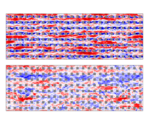
To gain insights into the instantaneous flow field, figure 2 displays the streamwise fluctuating velocity within and above the UCL from the HM case at two different  $x_3$ planes and phases. The chosen phases, $t=0$ and $t=T/2$, correspond to the end of the deceleration ( $T/2 < t < T$) and acceleration ( $0 < t < T/2$) periods, respectively.

Figure 2. Normalized instantaneous streamwise fluctuating velocity field  $u^\prime _1/u_\tau$ at streamwise/cross-stream plane $x_3=2h$ (a,b) and $x_3=0.75h$ (c,d) from the HM case. Here $u_{\tau }=\sqrt {f_m L_3}$ is the friction velocity based on the mean pressure gradient. Panels (a,c) correspond to $t=0$, whereas panels (b,d) correspond to $t=T/2$.
It is apparent from figure 2(a,b) that meandering low-momentum ( $u_1^\prime <0$) streaks are flanked by adjacent high-momentum ( $u_1^\prime >0$) ones. Comparing these two, turbulence structures at $t=T/2$ appear smaller in size in both streamwise and spanwise directions. Additionally, within the UCL, apparent vortex shedding occurs on the lee side of the cubes at $t=T/2$, while it is less pronounced at $t=0$. This suggests that flow unsteadiness substantially modifies the flow field during the pulsatile cycle and is expected to impact the flow statistics.
For a more comprehensive understanding of the phase-averaged flow pattern, figure 3 displays vector plots of  $(\bar {u}_1, \bar {u}_2)$ at $x_3/h=0.75$ for the LL and HVH cases. These cases feature the weakest and strongest departures from the statistically stationary flow regime, and the authors have verified that they comprehensively capture the range of flow variability within the considered suite of simulations. Colours in the figure depict the signed wall-parallel swirl strength $\lambda$, providing a visualization of the phase-averaged vortex morphology. The definition of $\lambda$ is in line with the approach of Stanislas, Perret & Foucaut (Reference Stanislas, Perret and Foucaut2008) and Elsinga et al. (Reference Elsinga, Poelma, Schröder, Geisler, Scarano and Westerweel2012). The magnitude of $\lambda$ is the absolute value of the imaginary part of the eigenvalue of the reduced velocity gradient tensor $\boldsymbol{\mathsf{J}}_{12}$, which is
 \begin{equation} \boldsymbol{\mathsf{J}}_{12}=\left(\begin{array}{@{}ll@{}} {\partial \bar{u}_{1}}/{\partial x_{1}} & {\partial \bar{u}_{1}}/{\partial x_{2}}\\ {\partial \bar{u}_{2}}/{\partial x_{1}} & {\partial \bar{u}_{2}}/{\partial x_{2}} \end{array}\right) . \end{equation}
The sign of  $\lambda$ is determined by the vorticity component $\omega _3$ and differentiates regions of anticlockwise (positive) and clockwise (negative) swirling motions.

Figure 3. Vector plots of the phase-averaged velocity at the  $x_3/h=0.75$ wall-parallel plane from LL (a) and HVH (b) cases. Colour contours represent the wall-normal swirling strength $\lambda$.
As shown in figure 3(a), the LL case exhibits a consistent vortex distribution throughout the pulsatile cycle. Strong shear layers manifest at the leading edges of the cuboid element, and the wake region is characterized by a pair of counter-rotating vortices. Such a vortex pair corresponds to an arch- or horseshoe-type vortex arising from the merging of recirculation vortices, which originate at the trailing edges of the top and sidewalls of the roughness element. It has been frequently observed in the wake of obstacles with height–width aspect ratios near unity. For further details, the reader is referred to Martinuzzi & Tropea (Reference Martinuzzi and Tropea1993), Pattenden, Turnock & Zhang (Reference Pattenden, Turnock and Zhang2005) and Gonçalves et al. (Reference Gonçalves, Franzini, Rosetti, Meneghini and Fujarra2015). In marked contrast, flow unsteadiness considerably modifies the flow pattern in the HVH case. Specifically, during the flow deceleration, the shear layers at the leading edges vanish due to flow reversal, i.e.  $\bar {u}_1<0$. During flow deceleration, the strength of the vortex pair is attenuated as its cores separate and distance themselves from the cuboid element, and the process is reversed during the acceleration. This behaviour is in line with findings from wind tunnel experiments of pulsatile flow over an isolated cube by Carr & Plesniak (Reference Carr and Plesniak2017).
Further insight can be obtained by considering variations in the normalized phase-averaged streamwise velocity, which are shown in figure 4 over a vertical transect for the LL and HVH cases. Acceleration and deceleration periods are apparent from the variations of the colour intensity in the above-UCL region, with the largest phase-averaged velocity magnitudes characterizing the end of the acceleration period, and lower ones the end of the deceleration. Dashed lines in figure 4 highlight that the flow is rather homogeneous above the UCL throughout the cases and that flow pulsation has a weak impact on the thickness of the roughness sublayer. Within the UCL, the LL case features modest variations in the structure of the phase-averaged streamwise velocity field; such a quantity retains approximately the same spatial structure throughout the pulsatile cycle and only varies in magnitude, with larger magnitudes occurring at  $t = T/2$. Phase variations in the phase-averaged streamwise velocity become again more apparent and interesting as the forcing frequency and amplitude increase, with the HVH case featuring ample regions of negative phase-averaged velocity at $t=0$ (end of flow deceleration) and $t = 3T/4$ (decelerating flow), and nearly lack thereof at $T/4$ (accelerating flow). Further, the largest negative phase-averaged velocity within the UCL occurs at $t = 3T/4$ rather than at $T/2$ as for the LL case, highlighting the presence of a different coupling between the UCL and the flow aloft. Note that all of the considered cases feature a relatively strong shear layer separating from the trailing edge of the cube, leading to enhanced local production of turbulent kinetic energy and transition from surface layer (above $h$) to canopy layer dynamics within the UCL. These observations, while still qualitative in nature, provide a first glimpse on complexities associated with the considered flow system and how it responds to a range of forcing amplitudes and frequencies. The next sections will delve into a more detailed quantitative analysis.

Figure 4. Phase-averaged streamwise velocity  $\bar {u}_1/u_{\tau }$ at the streamwise/vertical plane through the centre of the cube, i.e. $x_2=1.5h$, for low-amplitude cases: LL (a) and HVH (b). The fields depicted in different panels are $T/4$ apart. Solid contour lines denote $\bar {u}_1/u_{\tau }=0$. Dashed contour lines represent $\bar {u}_1=\bar {u}_1(0,1.5h,2h)$.
3.2. Longtime-averaged statistics
3.2.1. Longtime-averaged velocity profile
Profiles of the longtime-averaged streamwise velocity are shown in figure 5. Flow unsteadiness leads to a horizontal shift of profiles in the proposed semilogarithmic plot. This behaviour is distinct from the ‘two-log’ profile in flow over sand grain roughness (Fredsøe et al. Reference Fredsøe, Andersen and Sumer1999; Yang et al. Reference Yang, Tan, Lim and Zhang2006; Yuan & Madsen Reference Yuan and Madsen2015), and also in stark contrast to the one previously observed in current-dominated pulsatile flow over aerodynamically smooth surfaces, where the longtime-averaged field is essentially unaffected by flow unsteadiness (Tardu & Binder Reference Tardu and Binder1993; Scotti & Piomelli Reference Scotti and Piomelli2001; Tardu Reference Tardu2005; Manna et al. Reference Manna, Vacca and Verzicco2012; Weng et al. Reference Weng, Boij and Hanifi2016). As also apparent from figure 5, departures from the statistically stationary flow profile become more significant for larger values of  $\alpha$ and $\omega$.

Figure 5. Wall-normal profiles of longtime-averaged streamwise velocity  $\langle \bar {u}_1\rangle _l$ of high-amplitude cases (a) and low-amplitude cases (b). Line colour specifies the forcing frequency: navy blue, $\omega T_{h}=0.05{\rm \pi}$; dark green, $\omega T_{h}=0.125{\rm \pi}$; light green, $\omega T_{h}=0.25{\rm \pi}$; yellow-green, $\omega T_{h}=1.25{\rm \pi}$. Here $\langle \bar {u}_1\rangle$ from the SS case, represented by the red dashed line, is included for comparison. Black solid line indicates the slope of $1/\kappa$, with $\kappa =0.4$. The shaded area highlights the fitting region for the estimation of the roughness length scale $z_0$.
Variations in the aerodynamic roughness length  $z_0$ and displacement height $d$ parameters with $\omega T_h$ are shown in figure 6 for the considered canopy. These parameters are evaluated via the Macdonald et al. (Reference Macdonald, Griffiths and Hall1998) approach, where $d$ is the barycentre height of the longtime-averaged pressure drag from the urban canopy, and $z_0$ is determined via curve fitting. More specifically,
 \begin{equation} d = \frac{\int^h_0 \langle \bar{D} \rangle_l (x_3)x_3 \,{\rm d}\kern0.7pt x_3 }{\int^h_0 \langle \bar{D} \rangle_l (x_3 )\,{\rm d}\kern0.7pt x_3 }, \end{equation}
where the wall-normal distribution of the instantaneous canopy pressure drag  $D$ is obtained by taking an intrinsic volume average of the pressure gradient, i.e.
 \begin{equation} D(x_3,t) =\frac{1}{V_f}\int_{x_3-\delta z/2}^{x_3+\delta z/2}\int_0^{L_2} \int_0^{L_1}\frac{1}{\rho}\frac{\partial p}{\partial x} \,{\rm d}\kern0.7pt x_1 \,{\rm d}\kern0.7pt x_2 \,{\rm d}\kern0.7pt x_3. \end{equation}
Figure 6. Normalized aerodynamic roughness length  $z_0$ (a) and displacement height $d$ (b). Different colours correspond to different oscillation amplitudes: blue, $\alpha =0.2$; red, $\alpha =0.4$. The black square symbol denotes the reference SS case.
Note that, in principle, one should also account for the SGS drag contribution in (3.3); in this work, we omit SGS contributions because they are negligible when compared with the total drag – a direct result of the relatively small aerodynamic roughness length that is prescribed in the wall-layer model (see § 2.1).
Here  $z_0$ is solved by minimizing the root mean square error between the longtime-averaged velocity and the law of the wall with $\kappa =0.4$ in the $x_3 \in [2h,6h]$ interval, i.e.
 \begin{equation} E=\left\| \langle \bar{u}_1\rangle _{l}-\frac{u_{\tau}}{\kappa}\log\left(\frac{x_3-d}{z_0}\right)\right\|_{2} . \end{equation}
 The fitting interval is highlighted in figure 5. The estimated  $z_0$ was found to be poorly sensitive to variations in the fitting interval within the considered range of values. Cheng et al. (Reference Cheng, Hayden, Robins and Castro2007) argued that MacDonald's method is accurate when surfaces are characterized by a low packing density – a requirement that is indeed satisfied in the considered cases.
As apparent from figure 6,  $d$ is poorly sensitive to variations in both $\alpha$ and $\omega$ (variations across cases are within the $\pm 3\,\%$ range). This behaviour can be explained by considering that for flows over sharp-edged obstacles, such as the ones considered herein, flow separation consistently takes place at the sharp edges, irrespective of variations in $\alpha$ and $\omega$. This results in a similar net pressure distribution on the faces of the cuboids across all the considered cases. This can be readily observed in figure 4. The $d$ parameter is here evaluated as the integral of the pressure gradient field over the surface area, so the above considerations provide a physical justification for the observed behaviour. Note that this finding might not be generalizable across all possible roughness morphologies. For instance, Yu et al. (Reference Yu, Rosman and Hench2022) showed that separation patterns in pulsatile flows over hemispheres feature a rather strong dependence on $\alpha$ and $\omega$, yielding corresponding strong variations in $d$.
$d$.
Contrary to  $d$, the $z_0$ parameter is strongly impacted by flow unsteadiness, and its value increases with $\alpha$ and $\omega$. Bhaganagar (Reference Bhaganagar2008) reported a similar upward shift of velocity profile in his simulations of pulsatile flow over transitionally rough surfaces at a low Reynolds number. She attributed the increase in $z_0$ to the resonance between the unsteady forcing and the vortices shed by roughness elements, which is induced when the forcing frequency approaches that of the vortex shedding. However, such an argument does not apply to the cases under investigation, since we observed no spurious peaks in the temporal streamwise velocity spectrum. Rather, the increase in $z_0$ stems from the quadratic relation between the phase-averaged canopy drag and velocity, as elaborated below.
3.2.2. Phase-averaged drag-velocity relation
The phase-averaged canopy drag  $\langle \bar {D}\rangle$ and the local phase- and intrinsic-averaged velocity $\langle \bar {u}_1 \rangle$ at $x_3/h\approx 0.8$ are shown in figure 7, and are representative of corresponding quantities at different heights within the UCL. Results from cases with three lower frequencies and that from the SS case cluster along a single curve, highlighting the presence of a frequency-independent one-to-one mapping between $\langle \bar {D}\rangle$ and $\langle \bar {u}_1 \rangle$. As apparent from figure 8(a), at these three forcing frequencies, the interaction between the wind and the canopy layer is in a state of quasiequilibrium, i.e. $\langle \bar {D}\rangle$ is in phase with $\langle \bar {u}_1 \rangle$. Moreover, the shape of the aforementioned curve generally resembles the well-known quadratic drag law, which is routinely used to parameterize the surface drag in reduced-order models for stationary flow over plant and urban canopies (Lettau Reference Lettau1969; Raupach Reference Raupach1992; Macdonald et al. Reference Macdonald, Griffiths and Hall1998; Coceal & Belcher Reference Coceal and Belcher2004; Katul et al. Reference Katul, Mahrt, Poggi and Sanz2004; Poggi, Katul & Albertson Reference Poggi, Katul and Albertson2004). This finding comes as no surprise, given the quasiequilibrium state of the $\langle \bar {D}\rangle -\langle \bar {u}_1 \rangle$ relation for the three lower forcing frequencies.

Figure 7. Phase-averaged canopy drag  $\langle \bar {D} \rangle$ at $x_3/h\approx 0.8$ as a function of the local phase- and intrinsic-averaged velocity $\langle \bar {u}_1 \rangle$ (a) and the same $\langle \bar {D} \rangle -\langle \bar {u}_1 \rangle$ plot but with the time lag between $\langle \bar {D} \rangle$ and $\langle \bar {u}_1 \rangle$ removed (b). Different colours are used to denote different forcing frequencies: navy blue, $\omega T_{h}=0.05{\rm \pi}$; dark green, $\omega T_{h}=0.125{\rm \pi}$; light green, $\omega T_{h}=0.25{\rm \pi}$; yellow-green, $\omega T_{h}=1.25{\rm \pi}$. Different symbols are used to distinguish between oscillation amplitudes: triangle, $\alpha =0.2$; cross, $\alpha =0.4$. Red square represents the SS case. Red dashed line represents $\langle \bar {D} \rangle =C_d\lambda _f \langle \bar {u}_1 \rangle | \langle \bar {u}_1 \rangle |$ with $C_d$ obtained from the SS case.

Figure 8. Time evolution of  $\langle \bar {D} \rangle$ (black solid lines) and $\langle \bar {u}_1 \rangle$ (red dashed lines) at $x_3/h\approx 0.8$ from the HL (a) and LVH (b) cases. The acronyms of LES runs are defined in table 1.
On the other hand, as shown in figure 8(b), results from the highest-frequency cases (LVH and HVH) exhibit an orbital pattern, which stems from the time lag between  $\langle \bar {D} \rangle$ and $\langle \bar {u}_1 \rangle$. Artificially removing this time lag indeed yields a better clustering of data points from the highest-frequency cases along the quadratic drag law (see figure 7b).
These findings suggest the following parameterization for  $\langle \bar {D} \rangle$:
 \begin{equation} \langle \bar{D} \rangle(x_3,t)= C_d(x_3) \lambda_f \langle \bar{u}_1 \rangle \left | \langle \bar{u}_1 \rangle \right |(x_3,t+\Delta t) , \end{equation}
where  $C_d$ is a sectional drag coefficient that is constant in time and does not depend on $\alpha$ or $\omega$, and $\Delta t$ accounts for the time lag between $\langle \bar {D} \rangle$ and $\langle \bar {u}_1 \rangle$, which instead does indeed depend on $\alpha$ and $\omega$. Note that, throughout the considered cases, the wall-normal-averaged drag coefficient $\int ^{h}_0 C_d \,{\rm d}\kern0.7pt x_3/h\approx 0.9$ – a value that is similar to those previously reported ones for stationary flow over cube arrays (Coceal & Belcher Reference Coceal and Belcher2004) (note that the exact value depends on the formula used to define $C_d$).
Morison, Johnson & Schaaf (Reference Morison, Johnson and Schaaf1950) developed a semiempirical model relating the phase-averaged drag generated by obstacles in an oscillatory boundary layer to a given phase- and intrinsic-averaged velocity – a model that has been extensively used in the ocean engineering community to evaluate drag from surface-mounted obstacles (Lowe, Koseff & Monismith Reference Lowe, Koseff and Monismith2005; Yu, Rosman & Hench Reference Yu, Rosman and Hench2018; Yu et al. Reference Yu, Rosman and Hench2022). The Morison model assumes that the total force applied to the fluid by obstacles consists of a quadratic drag term and an inertial term; the latter accounts for the added mass effect and the Froude–Krylov force arising as a direct consequence of the unsteady pressure field. While it might seem plausible to utilize the Morison model to evaluate surface drag as a function of phase-averaged velocity at a given  $x_3$ for the cases under consideration, unfortunately, this approach is not applicable. As shown in Patel & Witz (Reference Patel and Witz2013), the Morison model provides relatively accurate evaluations of obstacle drag when the phased-averaged acceleration at different $x_3$ are in phase. This is not the case in this study, where substantial phase lags between phase-averaged accelerations at different wall-normal locations substantially degrade the accuracy of such a model. This behaviour can be easily inferred from the results in § 3.3.
In the following, we will make use of (3.5) to derive an alternative phenomenological surface-drag model for the considered flow system.
3.2.3. Mapping roughness length variability to longtime-averaged flow statistics
Here  $z_0$ and $d$ are input parameters of surface flux parameterizations that are routinely used in numerical weather prediction, climate projection and pollutant dispersion models (see, e.g. Skamarock et al. Reference Skamarock, Klemp, Dudhia, Gill, Barker, Duda, Huang, Wang and Powers2008; Benjamin et al. Reference Benjamin2016). These models are typically based on Reynolds-averaged Navier–Stokes closures, and feature time steps that can go from one hour up to several days. When departures from stationarity occur at a time scale that is much smaller than the time step of the model, model predictions are essentially longtime-averaged quantities, and the validity of surface flux parameterizations based on flow homogeneity and stationarity assumptions may break down. As a first step towards addressing this problem, this section proposes a phenomenological model relating $z_0$ to longtime-averaged pulsatile-flow statistics.
The longtime-averaged friction velocity can be written as
 \begin{equation} u^2_{\tau}=\int^{h}_0 \langle \bar{D} \rangle_l \,{\rm d}\kern0.7pt x_3=\int^{h}_0 C_d \lambda_f \langle \overline{\langle \bar{u}_1 \rangle \left | \langle \bar{u}_1 \rangle \right |}\rangle_l\,{\rm d}\kern0.7pt x_3 , \end{equation}
where  $\langle \bar {D} \rangle _l$ is the longtime-averaged surface drag. Note that the wall-normal structure of $C_d$ is approximately constant in the UCL (not shown here), except in the vicinity of the surface, where local contributions to the overall drag are, however, minimal due to the small value of $\langle \bar {u}_1 \rangle$. Thus, it is reasonable to assume $C_d$ is constant along the wall-normal direction. Also, depending on $\alpha$ and $\omega$, the flow within the canopy might undergo a local reversal in the phase- and intrinsic-averaged sense, meaning that $\langle \bar {u}_1 \rangle < 0$ at selected $x_3$ locations. Assuming that there is no flow reversal within the UCL, i.e. $\langle \bar {u}_1 \rangle \ge 0$ in $x_3 \le h$, (3.6) can be written as
 \begin{equation} u_{\tau}^2= C_d \lambda_f \left( \int^{h}_{0}{\langle \bar{u}_1\rangle_l^2}\,{{\rm d}\kern0.7pt x_3} + \int^{h}_{0}{\langle\overline{\langle \bar{u}_1\rangle_o ^2}\rangle_l}\,{{\rm d}\kern0.7pt x_3} \right) , \end{equation}
where the second term on the right-hand side of (3.7) is identically zero for the SS case. Equation (3.7) essentially states that an unsteady canopy layer requires a lower longtime-averaged wind speed to generate the same drag of a steady canopy layer since quadratic drag contributions are generated by flow unsteadiness (the second term on the right-hand side of (3.7)). Note that  $\sqrt {\int ^{h}_0 ({\cdot })^2\, {\rm d}\kern0.7pt x_3/h }$ is an averaging operation over the UCL based on the $L_2$ norm. Rearranging terms in (3.7) leads to
 \begin{equation} \langle \bar{u}_1\rangle_{l,{avg}} = \sqrt{\frac{u^2_{\tau}}{C_d \lambda_f h} -\frac{1}{h} \int^{h}_{0}{\langle\overline{\langle \bar{u}_1\rangle_o ^2}\rangle_l}\,{{\rm d}\kern0.7pt x_3} } , \end{equation}
and
 \begin{equation} \langle \bar{u}_1\rangle_{l,{avg}}^{{SS}} = \sqrt{\frac{u^2_{\tau}}{C_d \lambda_f h}} , \end{equation}
for the pulsatile cases and the SS case, respectively. Here  $({\cdot })_{{avg}}$ denotes the canopy-averaged quantity, and $({\cdot })^{{SS}}$ represents a quantity pertaining to the SS case.
As discussed in § 3.2.1, flow unsteadiness yields a shift of the  $\langle \bar {u}_1\rangle _{l}$ profile with negligible variations in the $d$ parameters when compared with the stationary flow with the same $u_\tau$. In terms of the law-of-the-wall, this behaviour can be described as a variation in $z_0$, i.e.
 \begin{equation} \langle \bar{u}_1\rangle_{l,{avg}}^{{SS}}-\langle \bar{u}_1\rangle_{l,{avg}}=\frac{u_\tau}{\kappa}\log \left( \frac{x_3-d}{z_0^{{SS}}}\right)-\frac{u_\tau}{\kappa}\log \left( \frac{x_3-d}{z_0}\right) , \end{equation}
where (3.10) is valid for any  $x_3$ in the logarithmic region. The shift in the velocity profile is approximately constant for $x_3 \in [0,L_3]$, so one can write
 \begin{equation} \langle \bar{u}_1\rangle_l^{{SS}}-\langle \bar{u}_1\rangle_l \approx \langle \bar{u}_1\rangle_{l,{avg}}^{{SS}}-\langle \bar{u}_1\rangle_{l,{avg}} , \end{equation}
and substituting (3.8)–(3.10) into (3.11) finally yields
 \begin{equation} z_0=z_0^{{SS}} \exp \left[ \kappa \left(\sqrt{\frac{1}{C_d \lambda_f h}}-\sqrt{\frac{1}{C_d \lambda_f h}-\frac{\int^{h}_{0}{\langle\overline{\langle \bar{u}_1\rangle_o ^2}\rangle_l}\,{{\rm d}\kern0.7pt x_3}/h}{u^2_{\tau}}}\right)\right] . \end{equation}
Equation (3.12) is a diagnostic model relating variations in the  $z_0$ parameter to the UCL phase- and intrinsic-averaged velocity variance – a longtime-averaged quantity. The $z_0$ estimates from (3.12) are compared with LES results in figure 9, using $C_d = 0.9$. It is apparent that the proposed model is able to accurately evaluate $z_0$ for most of the considered cases. For the LVH, HH and HVW runs, $z_0$ is overestimated by the model; these departures are attributed to the presence of flow reversal in the UCL, which contradicts the model assumptions.


Equation (3.12) highlights that, in the absence of flow reversal,  $z_0$ can be described as a monotonically increasing function of the $\langle \bar {u}_1\rangle _o$ variance in the UCL. As explained at the beginning of this section, this finding is of high relevance from a flow modelling perspective, because it relates a longtime-averaged flow statistic to the $z_0$ parameter. Note that $z_0^{{SS}}$ can be accurately evaluated using any existing parameterization for stationary ABL flow over aerodynamically rough surfaces, including the Lettau (Reference Lettau1969), Raupach (Reference Raupach1992) and Macdonald et al. (Reference Macdonald, Griffiths and Hall1998) models. Further, $C_d = 0.9$ (see discussion in § 3.2.2) and $\lambda _f$ and $h$ are morphological parameters that are in general a priori available. In weather forecasting and climate models, $\langle \bar {u}_1\rangle _o$ is an SGS quantity and would hence have to be parameterized as a function of longtime-averaged statistics that the model computes or from available in-situ or remote sensing measurements.
3.2.4. Longtime-averaged resolved Reynolds stress
This section shifts the attention to longtime-averaged resolved Reynolds stresses. For all of the considered cases, contributions from SGS stresses account for  $<1\,\%$ of the total phase-averaged Reynolds stresses and are hence not discussed.
Throughout the boundary layer,  $\langle \overline {u_1^\prime u_3^\prime }\rangle _l$ profiles are indistinguishable from the SS one (not shown), indicating a weak dependence of such a quantity on $\alpha$ and $\omega$. Above the UCL, the divergence of $\langle \overline {u_1^\prime u_3^\prime }\rangle _l$ balances the longtime-averaged driving pressure gradient $f_m$, i.e.
 \begin{equation} -\frac{\partial \langle\overline{u_1^\prime u_3^\prime}\rangle_l}{\partial x_3}+f_m=0 . \end{equation}
Since  $f_m$ does not vary across the considered cases and $\langle \overline {u_1^\prime u_3^\prime }\rangle _l(L_3) = 0$, a collapse of $\langle \overline {u_1^\prime u_3^\prime }\rangle _l$ profiles in this region was to be expected from the mathematical structure of the governing equations. Within the UCL, the longtime-averaged momentum budget reads
 \begin{equation} -\frac{\partial \langle\overline{u_1^\prime u_3^\prime}\rangle_l}{\partial x_3}+f_m-\langle\bar{D}\rangle_l=0 . \end{equation}
Given that  $\langle \overline {u_1^\prime u_3^\prime }\rangle _l$ profiles collapse in this region, $\langle \bar {D}\rangle _l$ is also expected to feature a weak dependence on $\alpha$ and $\omega$, which in turn explains the weak variations in the $d$ parameter that were observed in § 3.2.1.
Figure 10 depicts wall-normal profiles of the longtime-averaged resolved turbulent kinetic energy, which is defined as
 \begin{equation} \langle\bar{k}\rangle_l=\tfrac{1}{2}(\langle\overline{u_1^\prime u_1^\prime}\rangle_l+\langle\overline{u_2^\prime u_2^\prime}\rangle_l+\langle \overline{u_3^\prime u_3^\prime}\rangle_l) . \end{equation}
Such a quantity features a significant increase in the UCL when compared with its values farther away from the surface, which as discussed in Schmid et al. (Reference Schmid, Lawrence, Parlange and Giometto2019), is due to dispersive contributions caused by the canopy geometry. Flow unsteadiness has a relatively more important impact on such a quantity when compared with the  $\langle \overline {u_1^\prime u_3^\prime }\rangle _l$ component, especially for flow in the UCL and for cases with a high oscillation amplitude. An increase in $\alpha$ generally results in more pronounced departures of $\langle \bar {k}\rangle _l$ profiles from the SS one. This behaviour can be best explained by considering the shear production terms in the budget equation for $\langle \bar {k}\rangle _l$, i.e.
 \begin{equation} \langle \bar{\mathcal{P}}\rangle_l={-}\left\langle\overline{\langle \overline{u_1^\prime u_3^\prime} \rangle \frac{\partial \langle \bar{u}_1 \rangle }{\partial x_3}}\right\rangle_l=\underbrace{-\langle \overline{ u_1^\prime u_3^\prime}\rangle_l \frac{\partial\langle \bar{u}_1\rangle_l }{\partial x_3}}_{\langle \bar{\mathcal{P}}\rangle_{l,1}}\underbrace{-\left\langle\overline{\langle\overline{ u_1^\prime u_3^\prime }\rangle_o \frac{\partial \langle\bar{u}_1\rangle_o }{\partial x_3}}\right\rangle_l} _{\langle \bar{\mathcal{P}}\rangle_{l,2}} , \end{equation}
where  $\langle \bar {\mathcal {P}}\rangle _{l,1}$ represents the work done by $\langle \overline { u_1^\prime u_3^\prime }\rangle _l$ onto the longtime-averaged flow field, and ${\langle \bar {\mathcal {P}}\rangle _{l,2}}$ is the longtime average of the work done by the oscillatory shear stress $\langle \overline { u_1^\prime u_3^\prime }\rangle _o$ onto the oscillatory flow field. Figure 11(a) shows that $\langle \bar {\mathcal {P}}\rangle _{l,1}$ is poorly sensitive to variations in $\alpha$ and $\omega$. This behaviour stems from the constancy of $\langle \overline { u_1^\prime u_3^\prime }\rangle _l$ and ${\partial \langle \bar {u}_1\rangle _l }/{\partial x_3}$ across cases (the latter can be inferred from the systematic shift of $\langle \bar {u}_1\rangle _l$ profiles in figure 5). Conversely, $\langle \bar {\mathcal {P}}\rangle _{l,2}$ from high-amplitude cases are generally larger than those from low-amplitude ones, mainly due to the higher $\langle \overline { u_1^\prime u_3^\prime }\rangle _o$ and $\langle \bar {u}_1\rangle _o$ values. Discrepancies in $\langle \bar {\mathcal {P}}\rangle _{l,2}$ among high-amplitude cases are larger than those among low-amplitude ones, which ultimately yields the observed variability in $\langle \bar {k}\rangle _l$.

Figure 10. Longtime-averaged resolved turbulent kinetic energy  $\langle \bar {k}\rangle _l=(\langle \overline {u_1^\prime u_1^\prime }\rangle _l+\langle \overline {u_2^\prime u_2^\prime }\rangle _l+\langle \overline {u_3^\prime u_3^\prime }\rangle _l)/2$ from high-amplitude cases (a) and low-amplitude cases (b). Line colours correspond to those used in figure 5.

Figure 11. Normalized shear production terms of  $\langle \bar {k}\rangle _l$: $\langle \bar {\mathcal {P}}\rangle _{l,1}$ (a) and $\langle \bar {\mathcal {P}}\rangle _{l,2}$ (b). Symbols and line colours correspond to those used in figure 7.
Further insight into the problem can be gained by looking at the normal components of the longtime-averaged resolved Reynolds stress tensor, which are shown in figure 12. In this case, it is apparent that increases in the oscillation frequency lead to a decrease in  $\langle \overline {u_1^\prime u_1^\prime }\rangle _l$ and an increase in $\langle \overline {u_2^\prime u_2^\prime }\rangle _l$ and $\langle \overline {u_3^\prime u_3^\prime }\rangle _l$ within the UCL – a behaviour that is especially apparent for the high-amplitude cases (figure 12d–f). These trends can be best understood by examining the pressure-strain terms from the budget equations of the longtime-averaged resolved Reynolds stresses, i.e.
 \begin{equation} {\mathsf{R}}_{ij} = \left\langle\overline{\frac{p^\prime}{\rho} \left(\frac{\partial u^\prime_j}{\partial x_i}+\frac{\partial u^\prime_i}{\partial x_j}\right)}\right\rangle_l. \end{equation}
Figure 12. Longtime-averaged resolved normal Reynolds stresses  $\langle \overline {u_1^\prime u_1^\prime }\rangle _l$, $\langle \overline {u_2^\prime u_2^\prime }\rangle _l$ and $\langle \overline {u_3^\prime u_3^\prime }\rangle _l$ from low-amplitude cases (a–c) and high-amplitude cases (d–f). Line colours correspond to those used in figure 5.
Here  $R_{ii}$ are responsible for redistributing kinetic energy among the longtime-averaged normal Reynolds stresses (Pope Reference Pope2000), and are shown in figure 13. With the exception of the very near surface region ( $x_3 \lessapprox 0.2$) where no clear trend can be observed, increases in $\omega$ and $\alpha$ yield a decrease in ${\mathsf{R}}_{11}$ and an increase in ${\mathsf{R}}_{22}$ and ${\mathsf{R}}_{33}$, which justify the observed isotropization of turbulence in the UCL.

Figure 13. Pressure redistribution terms  ${\mathsf{R}}_{ii}$: (a–c) low-amplitude cases; (d–f) high-amplitude cases. Line colours correspond to those used in figure 5.
3.3. Oscillatory fields
This section shifts the focus to the time evolution of velocity and resolved Reynolds stresses during the pulsatile cycle.
3.3.1. Oscillation amplitude impacts on the oscillatory fields
Flow statistics from the LL and HL simulations are here examined to study the impact of the oscillation amplitude  $(\alpha )$ on the oscillatory velocity and resolved Reynolds stresses. Only the LL and HL runs are discussed, as they were found to be representative of the observed behaviours for the other low and high-amplitude cases, respectively.
Figure 14 contrasts the profiles of oscillatory velocity  $(\langle \bar {u}_1\rangle _o)$ from the LL and HL runs at four equispaced phases during the pulsatile cycle. The $\langle \bar {u}_1\rangle _o$ at the top of the domain is controlled by the $\alpha$ parameter, so it is natural to use $u_{\tau }\alpha$ as a normalization constant to study the problem. Manna et al. (Reference Manna, Vacca and Verzicco2012) investigated pulsatile open channel flow over an aerodynamically smooth surface, and showed that using such a normalization constant is indeed convenient as it leads to a collapse of $\langle \bar {u}_1\rangle _o$ profiles across cases with different amplitudes, even in the presence of strong flow reversal. This indicates that, at a given forcing frequency, the amplitude of the oscillatory velocity within the domain is proportional to that at the top of the domain. In this work, we show that such a scaling works well also in the presence of aerodynamically rough surfaces, as evidenced by the excellent collapse of $\langle \bar {u}_1\rangle _o/(u_{\tau }\alpha )$ profiles in figure 14. This is not trivial, especially when considering the different scaling of surface drag between aerodynamically smooth and rough walls in the presence of flow unsteadiness.

Figure 14. Profiles of the oscillatory velocity  $\langle \bar {u}_1\rangle _o$ from the LL (blue) and HL (red) cases at different phases of the pulsatile cycle. Profiles are $T/4$ apart.
The oscillatory resolved turbulent kinetic energy can be defined as
 \begin{equation} \langle\bar{k}\rangle_o=\tfrac{1}{2}\big(\langle\overline{u_1^\prime u_1^\prime}\rangle_o+\langle\overline{u_2^\prime u_2^\prime}\rangle_o+\langle\overline{u_3^\prime u_3^\prime}\rangle_o\big) . \end{equation}
As shown in figures 15 and 16, both the oscillatory resolved Reynolds shear stress  $\langle \overline {u_1^\prime u_3^\prime }\rangle _o$ and $\langle \bar {k}\rangle _o$ scale with $u_{\tau }^2 \alpha$. Although not shown, the three oscillatory normal Reynolds stresses also obey such a scaling, suggesting that any change in $\langle \bar {k}\rangle _o$ is proportionally distributed to the three normal Reynolds stresses during the pulsatile cycle. As discussed in the following paragraphs, the scaling of $\langle \overline {u_1^\prime u_3^\prime }\rangle _o$ and $\langle \bar {k}\rangle _o$ is a direct consequence of the mild nonlinearity in the production of $\langle \bar {k}\rangle _o$ and $\langle \overline {u_1^\prime u_3^\prime }\rangle _o$. Subtracting the budget equation of $\langle \overline {u_1^\prime u_3^\prime }\rangle _l$ from that of $\langle \overline {u_1^\prime u_3^\prime } \rangle$, one obtains
 \begin{align} \frac{\partial \langle\overline{u_1^\prime u_3^\prime}\rangle_o}{\partial t}= & \underbrace{-2\langle\overline{u_3^\prime u_3^\prime}\rangle_o \frac{\partial \langle\bar{u}_1 \rangle_l}{\partial x_3}}_{\langle \bar{\mathcal{P}}_{13}\rangle_{o,l1}} \underbrace{-2\langle\overline{u_3^\prime u_3^\prime}\rangle_l \frac{\partial \langle\bar{u}_1 \rangle_o}{\partial x_3}}_{\langle \bar{\mathcal{P}}_{13}\rangle_{o,l2}}\nonumber\\ & \underbrace{-2\langle\overline{u_3^\prime u_3^\prime}\rangle_o \frac{\partial \langle\bar{u}_1 \rangle_o }{\partial x_3}+2\left\langle\overline{\langle\overline{u_3^\prime u_3^\prime}\rangle_o \frac{\partial \langle\bar{u}_1 \rangle_o }{\partial x_3}}\right\rangle_l}_{\langle \bar{\mathcal{P}}_{13}\rangle_{o,nl}}+\cdots, \end{align}
where  $\langle \bar {\mathcal {P}}_{13}\rangle _{o,l1}$ and $\langle \bar {\mathcal {P}}_{13}\rangle _{o,l2}$ are the linear production terms of $\langle \overline {u_1^\prime u_3^\prime }\rangle _o$, while $\langle \bar {\mathcal {P}}_{13}\rangle _{o,nl}$ is the nonlinear production. Similarly, the budget equations of $\langle \bar {k}\rangle _o$ can be written as
 \begin{equation} \frac{\partial \langle\bar{k}\rangle_o}{\partial t}= \underbrace{-\langle\overline{u_1^\prime u_3^\prime}\rangle_o \frac{\partial \langle\bar{u}_1 \rangle_l}{\partial x_3}}_{\langle \bar{\mathcal{P}}_{k}\rangle_{o,l1}} \underbrace{-\langle\overline{u_1^\prime u_3^\prime}\rangle_l \frac{\partial \langle\bar{u}_1 \rangle_o}{\partial x_3}}_{\langle \bar{\mathcal{P}}_{k}\rangle_{o,l2}} \underbrace{-\langle\overline{u_1^\prime u_3^\prime}\rangle_o \frac{\partial \langle\bar{u}_1 \rangle_o }{\partial x_3}+\left\langle\overline{\langle\overline{u_1^\prime u_3^\prime}\rangle_o \frac{\partial \langle \bar{u}_1 \rangle_o }{\partial x_3}}\right\rangle_l}_{\langle \bar{\mathcal{P}}_{k}\rangle_{o,nl}}+\cdots , \end{equation}
where  $\langle \bar {\mathcal {P}}_{k}\rangle _{o,l1}$ and $\langle \bar {\mathcal {P}}_{k}\rangle _{o,l2}$ are the linear production terms of $\langle \bar {k}\rangle _o$, while $\langle \bar {\mathcal {P}}_{k}\rangle _{o,nl}$ is the nonlinear production. As shown in figure 17, the nonlinear production term is substantially smaller than the sum of the corresponding linear productions for both $\langle \overline {u_1^\prime u_3^\prime }\rangle _o$ and $\langle \bar {k}\rangle _o$. Given that $\langle \overline {u_1^\prime u_3^\prime }\rangle _l$, $\langle \overline {u_3^\prime u_3^\prime }\rangle _l$ and ${\partial \langle \bar {u}_1\rangle _l}/{\partial x_3}$ from the LL and HL cases are similar, when $\langle \bar {u}_1\rangle _o \sim u_{\tau }\alpha$ and $\langle \overline {u_3^\prime u_3^\prime }\rangle _o\sim u_{\tau }^2 \alpha$, the total production of $\langle \overline {u_1^\prime u_3^\prime }\rangle _o$ is
 \begin{equation} \langle \bar{\mathcal{P}}_{13}\rangle_{o}\approx \langle \bar{\mathcal{P}}_{13}\rangle_{o,l1}+\langle \bar{\mathcal{P}}_{13}\rangle_{o,l2} \sim \frac{u_{\tau}^3 \alpha}{h} , \end{equation}
whereas that of  $\langle \bar {k}\rangle _o$ is
 \begin{equation} \langle \bar{\mathcal{P}}_{k}\rangle_{o}\approx \langle \bar{\mathcal{P}}_{k}\rangle_{o,l1}+\langle \bar{\mathcal{P}}_{k}\rangle_{o,l2} \sim \frac{u_{\tau}^3 \alpha}{h} . \end{equation}
This in turn leads to the observed  $\langle \overline {u_1^\prime u_3^\prime }\rangle _o \sim u_{\tau }^2 \alpha$ and $\langle \bar {k}\rangle _o \sim u_{\tau }^2 \alpha$ scalings.

Figure 15. Profiles of the oscillatory resolved Reynolds shear stress  $\langle \overline {u_1^\prime u_3^\prime }\rangle _o$ from the LL (blue) and HL (red) cases at different phases of the pulsatile cycle. Profiles are $T/4$ apart.

Figure 16. Profiles of the oscillatory resolved turbulent kinetic energy  $\langle \bar {k}\rangle _o=(\langle \overline {u_1^\prime u_1^\prime }\rangle _o+\langle \overline {u_2^\prime u_2^\prime }\rangle _o+\langle \overline {u_3^\prime u_3^\prime }\rangle _o)/2$ from the LL (blue) and HL (red) cases at different phases of the pulsatile cycle. Profiles are $T/4$ apart.

Figure 17. Normalized production terms for  $\langle \overline {u_1^\prime u_3^\prime }\rangle _o$ (a) and for $\langle \bar {k}\rangle _o$ (b) at $x_3/h=1.5$ from the LL (blue) and HL (red) cases. Solid lines denote the linear production terms, and dash lines represent the nonlinear production terms.
Equations (3.21) and (3.22) are expected to fail under two conditions. Firstly, when  $\alpha$ is sufficiently large and the contribution of $\langle \bar {\mathcal {P}}_{13}\rangle _{o,nl}$ and $\langle \bar {\mathcal {P}}_{k}\rangle _{o,nl}$ can no longer be neglected. Secondly, when differences in $\langle \overline {u_1^\prime u_3^\prime }\rangle _l$ or $\langle \overline {u_3^\prime u_3^\prime }\rangle _l$ among cases with different $\alpha$ become large enough that the linear production terms cease to scale with $u_{\tau }^2 \alpha$, which occurs within the UCL for the LVH and HVH cases (see figure 12).
The above analysis has shown that the  $\alpha$ parameter primarily controls the amplitude of selected oscillatory flow quantities, but has little impact on their wall-normal structure. In the next section, it will be shown that the wall-normal structure of quantities is instead controlled by $\omega$. This behaviour is also expected to hold in the smooth-wall set-up (Manna et al. Reference Manna, Vacca and Verzicco2012), although the mechanism responsible for generating drag over aerodynamically smooth surfaces is quite distinct.
3.3.2. Forcing frequency impacts on the oscillatory fields
This section discusses how the oscillatory velocity and resolved Reynolds stresses respond to variations in the forcing frequency. Only low-amplitude cases will be considered since conclusions can be generalized across the considered runs.
Figures 18 and 19 present the time evolution of  $\langle \bar {u}_1\rangle _o$ and $\partial \langle \bar {u}_1\rangle _o/\partial x_3$. Three distinct frequency regimes can be identified. The first regime corresponds to the highest amongst the considered forcing frequencies, i.e. the LVH case. For this flow regime, the oscillation in $\partial \langle \bar {u}_1\rangle _o/\partial x_3$ is typically confined within the UCL. This behaviour can be best explained when considering that the time period of the oscillation is comparable to the eddy turnover time of turbulence in the UCL, i.e. $T \approx T_h$, which is the characteristic time scale for ‘information transport’ within the UCL. At the three lower forcing frequencies, i.e. the LL, LM and LH cases, on the contrary, the interaction between the roughness elements and the unsteady flow induces an oscillation in the shear rate, which has a phase lag of roughly ${\rm \pi} /2$ with respect to the pulsatile forcing at the top of the UCL. This oscillating shear rate then propagates in the positive wall-normal direction while being progressively attenuated. The propagation speed of the oscillating shear rate appears to be constant for a given forcing frequency, which can be readily inferred by the constant tilting angle in the $\partial \langle \bar {u}_1\rangle _o/\partial x_3$ contours. The flow region affected by the oscillating shear rate defines the so-called ‘Stokes layer’. For cases with two moderate frequencies, i.e. the LM and LH cases, the Stokes layer thickness $(\delta _s)$ is smaller than the domain height $L_3$. Above the Stokes layer, the slope of $\langle \bar {u}_1\rangle _o$ is nominally zero over the pulsatile cycle, and the flow in such a region resembles a plug flow. On the contrary, in the LL case, the entire domain is affected by the oscillating shear rate, thus $\delta _s>L_3$.

Figure 18. Space–time diagrams of  $\langle \bar {u}_1\rangle _o/u_\tau$ from the LL (a), LM (b), LH (c) and LVH (d) cases. Horizontal dashed lines identify the top of the UCL.

Figure 19. Space–time diagrams of  $(h/u_\tau ) {\partial \langle \bar {u}_1\rangle _o}/{\partial x_3}$ from the LL (a), LM (b), LH (c) and LVH (d) cases.
Figures 20 and 21 depict the time evolution of  $\langle \overline {u_1^\prime u_3^\prime }\rangle _o$ and $\langle \overline {u_1^\prime u_1^\prime }\rangle _o$, respectively. Although the contours of $\langle \overline {u_2^\prime u_2^\prime }\rangle _o$ and $\langle \overline {u_3^\prime u_3^\prime }\rangle _o$ are not shown, these quantities vary in a similar fashion as $\langle \overline {u_1^\prime u_1^\prime }\rangle _o$ during the pulsatile cycle. These space–time diagrams confirm that the considered frequencies encompass three distinct flow regimes. For the LVH case, time variations of the oscillatory resolved Reynolds stresses are essentially zero above the UCL. In cases with three lower frequencies, oscillatory resolved Reynolds stresses exhibit a similar behaviour to $\partial \langle \bar {u}_1\rangle _o/\partial x_3$. Specifically, there appear oscillating waves propagating away from the UCL at a constant speed and meanwhile getting weakened. In the LM and LH cases, such oscillating waves are fully dissipated at the upper limit of the Stokes layer, above which the turbulence is ‘frozen’ and passively advected.

Figure 20. Space–time diagrams of  $\langle \overline {u_1^\prime u_3^\prime }\rangle _o / u_\tau ^2$ from the LL (a), LM (b), LH (c) and LVH (d) cases.

Figure 21. Space–time diagrams of  $\langle \overline {u_1^\prime u_1^\prime }\rangle _o/u_\tau ^2$ from the LL (a), LM (b), LH (c) and LVH (d) cases.
A visual comparison of the tilting angles in the contours of oscillatory resolved Reynolds stresses and  $\partial \langle \bar {u}_1\rangle _o/\partial x_3$ reveals that the oscillating waves in these quantities feature similar propagation speeds. This behaviour closely resembles the one observed in smooth-wall cases (Scotti & Piomelli Reference Scotti and Piomelli2001; Manna et al. Reference Manna, Vacca and Verzicco2015). The physical interpretation is that when the oscillating shear rate is diffused upwards by the background turbulent flow, it interacts with the local turbulence via the mechanisms described in (3.19) and (3.20), thus inducing the observed oscillations in the resolved Reynolds stresses. To further quantify the propagation speeds of the oscillating waves in ${\partial \langle \bar {u}_1\rangle _o}/{ \partial x_3}$ and oscillatory resolved Reynolds stresses, figure 22 presents the phase lag of those quantities with respect to the pulsatile forcing. For a quantity $\theta$, the propagation speed $c_\theta$ is defined based on the slope of the phase lag, i.e.
 \begin{equation} c_\theta={-} \omega\frac{\partial x_3}{\partial \phi_\theta} . \end{equation}
Figure 22. Phase lag of  ${\partial \langle \bar {u}_1\rangle _o}/{ \partial x_3}$ (red), $-\langle \overline {u_1^\prime u_3^\prime }\rangle _o$ (black), $\langle \overline {u_1^\prime u_1^\prime }\rangle _o$ (magenta), $\langle \overline {u_2^\prime u_2^\prime }\rangle _o$ (green) and $\langle \overline {u_3^\prime u_3^\prime }\rangle _o$ (blue) with respect to the pulsatile forcing from the LL (a), LM (b) and LH (c) cases.
Table 2 summarizes the wave propagation speeds for  $\partial \langle \bar {u}_1\rangle _o /\partial x_3$, $-\langle \overline { u_1^\prime u_3^\prime }\rangle _o$, $\langle \overline { u_1^\prime u_1^\prime }\rangle _o$, $\langle \overline { u_2^\prime u_2^\prime }\rangle _o$ and $\langle \overline { u_3^\prime u_3^\prime }\rangle _o$ of each case. This again confirms that the oscillating waves propagate at a similar speed for the considered quantities. It is also noteworthy to point out that the speed of the propagating wave increases with $\omega$.
Table 2. Propagation speeds of oscillating waves in  $\partial \langle \bar {u}_1\rangle _o /\partial x_3$ and oscillatory resolved Reynolds stresses.

Three other observations can be made from figure 22. First, throughout the considered cases, there appears a marked phase lag of roughly  ${\rm \pi} /6$ between $\partial \langle \bar {u}_1\rangle _o /\partial x_3$ and (negative) $\langle \overline {u_1^\prime u_3^\prime }\rangle _o$, indicating a deviation from the Boussinesq eddy viscosity assumption. Weng et al. (Reference Weng, Boij and Hanifi2016) reported a similar finding, and they attributed such behaviour to non-equilibrium effects arising when the time period of the pulsatile forcing is short compared with the local turbulence relaxation time so that the turbulence is not able to relax to its equilibrium state during the pulsation cycle. Second, the lack of phase lag among the oscillatory normal resolved Reynolds stresses implies that the oscillatory pressure-redistribution terms respond immediately to the change in $\langle \overline { u_1^\prime u_1^\prime }\rangle _o$. Third, the lifetimes of oscillating waves in the resolved Reynolds stresses and shear rate, which are inferred by the difference between the phase lags at the top of the UCL and at the upper limit of the Stokes layer, are no more than half of the oscillation time period, although they decrease with $\omega$. They are considerably shorter than those in smooth-wall cases, which are typically larger than one oscillation period (Scotti & Piomelli Reference Scotti and Piomelli2001; Manna et al. Reference Manna, Vacca and Verzicco2015; Weng et al. Reference Weng, Boij and Hanifi2016).
3.3.3. Scaling of the Stokes layer thickness
Across many applications,  $\delta _s$ is a quantity of interest, since it defines the region where the turbulence and the mean flow are out of equilibrium. In such a region, established turbulence theories may fail to capture flow dynamics that are of relevance for, e.g. surface drag and scalar dispersion.
For the wave-current boundary flow, where the surface is typically transitionally rough, the wave boundary layer thickness – an equivalent of Stokes layer thickness – scales as
 \begin{equation} \delta_w \sim \frac{\kappa u_{\tau,max}}{\omega} , \end{equation}
where  $u_{\tau,max}$ is the friction velocity based on the maximum phase- and intrinsic-averaged wall stress during the pulsatile cycle (Grant & Madsen Reference Grant and Madsen1979). Such a scaling argument is not valid for the current cases, even though the considered surface is also rough. As shown in § 3.3.1, normalized oscillatory velocity and resolved Reynolds stresses profiles collapse between cases with the same frequencies, implying that the Stokes layer thickness is only dependent on $\omega$, whereas $\tau _{max}$ is determined by both $\alpha$ and $\omega$. Rather, the scaling of $\delta _s$ in the current cases is a trivial extension of the model first introduced by Scotti & Piomelli (Reference Scotti and Piomelli2001), as discussed next.
Let us recall from § 1 that the Stokes layer thickness for turbulent pulsatile flow over an aerodynamically smooth surface (Scotti & Piomelli Reference Scotti and Piomelli2001) is defined as
 \begin{equation} \delta_s = 2\frac{\kappa u_\tau}{\omega}\left(1+\sqrt{1+ \frac{2\nu \omega}{\kappa^2 u_\tau^2}}\right) . \end{equation}
 Here we apply two modifications to this model in order to make it applicable to the current rough-wall cases. First, given that the viscous stress is omitted, the molecular viscosity  $\nu$ can be neglected. Also, in the current cases, the oscillating shear rate is generated within the UCL rather than at the bottom surface (as in the smooth-wall cases), and the extent of the oscillating shear rate propagation defines the thickness of the Stokes layer. This behaviour can be easily captured by augmenting $\delta _s$ by the displacement height ( $d$). Specifically, we draw an analogy to smooth-wall cases by taking $d$ as the offset, since it is the virtual origin of the longtime-averaged velocity profile. The displacement height, $d$, is a plausible choice of the offset since it captures the limiting behaviour of the flow system as the canopy packing density varies. For instance, in the limit of $\lambda _p \rightarrow 0$ (very sparse canopies), $d = 0$, i.e. the oscillating shear rate grows from the bottom of the domain. On the contrary, in the limit of $\lambda _p \rightarrow 1$ (very dense canopies), $d = h$, i.e. the oscillating shear layer starts at the top of the UCL. Based on these considerations, a phenomenological model for the Stokes layer thickness is
 \begin{equation} \delta_s=\frac{4\kappa u_\tau}{\omega}+d . \end{equation}
Note that, in the limit of  $\omega \rightarrow 0$, the Stokes layer no longer exists, rendering (3.26) invalid. At this limit, as previously stated in Scotti & Piomelli (Reference Scotti and Piomelli2001), $T$ is much larger than the turbulence relaxation time. As a result, the turbulence maintains a quasiequilibrium state, and the flow statistics are indistinguishable from those of the corresponding equilibrium canopy layer flows, if scaled with the instantaneous inner/outer units.
Figure 23 compares the predictions of (3.26) against LES results. Note that only low-amplitude cases are shown, since, as mentioned earlier,  $\delta _s$ only depends on $\omega$. The upper limit of the Stokes layer is identified as the location where $\sigma ^2_{ \langle \bar {k}\rangle _o}$ is $1\,\%$ of its maximum, where
 \begin{equation} \sigma^2_{ \langle\bar{k}\rangle_o}= \frac{1}{T}\int^{T}_0 \left(\frac{1}{2}\big(\langle\overline{ u_1^\prime u_1^\prime }\rangle_o+\langle\overline{ u_2^\prime u_2^\prime }\rangle_o+\langle\overline{ u_3^\prime u_3^\prime }\rangle_o\big)\right)^2 \,{\rm d}t \end{equation}
is the time variance of  $\langle \bar {k}\rangle _o$. From figure 23, it is apparent that the estimated $\delta _s$ compare very well with LES results. The estimation of $\delta _s$ for the LL case is not shown in figure 23 because it exceeds the height of the computational domain. Equation (3.26) can hence be used in future studies to identify the Stokes layer thickness for pulsatile flows over aerodynamically rough surfaces.

Figure 23. Time variance of  $\langle \bar {k}\rangle _o$: $\sigma ^2_{ \langle \bar {k}\rangle _o}=\int ^{T}_0 \big(\tfrac {1}{2} \big(\langle \overline { u_1^\prime u_1^\prime }\rangle _o+\langle \overline { u_2^\prime u_2^\prime }\rangle _o+\langle \overline { u_3^\prime u_3^\prime }\rangle _o\big)\big)^2 \,{\rm d}t/T$ of the LL (navy blue), LM (dark green), LH (light green) and LVH (yellow green) cases. Circle denotes $\delta _s$ estimated via (3.26). Triangle represents the location where $\sigma ^2_{ \langle \bar {k}\rangle _o}$ is reduced to $1\,\%$ of its maximum value.
4. Conclusions
This paper has examined the impact of flow pulsation on longtime-averaged and phase-dependent flow statistics in an open-channel flow over urban-like roughness. A series of LES of pulsatile flow past an array of cuboid elements has been carried out, programmatically varying the oscillation amplitude  $(\alpha )$ and frequency $(\omega )$. The forcing frequencies have been chosen as a multiple of the characteristic frequency of turbulence in the UCL and encompass a range of values representative of submesoscale motions (Mahrt & Bou-Zeid Reference Mahrt and Bou-Zeid2020). The main findings and contributions of this study are outlined below.
(i) Flow pulsation leads to an increase of the $z_0$ parameter educed from longtime-averaged $\langle \bar {u}_1\rangle _l$ profiles, with larger $\alpha$ and $\omega$ values yielding a larger $z_0$. On the contrary, $d$ was found to be insensitive to variations in $\alpha$ and $\omega$. The increase of $z_0$ was shown to be a direct consequence of the quadratic relation between the phase-averaged canopy drag $\langle \bar {D} \rangle$ and the phase- and intrinsic-averaged velocity $\langle \bar {u}_1\rangle$, and this relation was leveraged to construct a phenomenological model for $z_0$. The proposed model takes surface information and the variance of the phase- and intrinsic-averaged velocity in the UCL as input parameters and captures the impact of flow unsteadiness on the $z_0$ parameter in the absence of flow reversal.
(ii) The wall-normal distributions of the longtime-averaged shear stress and canopy drag are unaltered by the flow unsteadiness. In contrast, the same cannot be said for longtime-averaged resolved normal Reynolds stresses, especially in the UCL. In particular,
$\langle \bar {k}\rangle _l$ profiles were found to be relatively more sensitive to variations in $\alpha$ via the longtime-averaged shear production of $\langle \bar {k}\rangle _l$. The highest frequency cases were also characterized by a relatively more isotropic turbulence field in the UCL, owing to a more efficient kinetic energy redistribution by the pressure-strain terms.(iii) The oscillation amplitudes of phase- and intrinsic-averaged streamwise velocity and resolved Reynolds stresses scale with
$\alpha$. This behaviour is due to the fact that the nonlinear production terms of $\langle \overline {u_1^\prime u_3^\prime }\rangle _o$ and $\langle \bar {k}\rangle _o$ are of relatively modest magnitude when compared with the linear ones. Increasing the pulsation amplitude might lead to more substantial contributions from nonlinear production terms and break down this scaling.(iv) For each case, profiles of oscillatory shear rate and resolved Reynolds stresses are characterized by oscillating waves which are advected away from the UCL at a constant speed while also being dissipated. Here
$\omega$ is found to determine both the speeds of the oscillating waves and the extent of these waves, which identifies the Stokes layer thickness $(\delta _s)$. More specifically, $\delta _s$ was found to increase with decreasing $\omega$, whereas the wave speed increased with $\omega$. The scaling of $\delta _s$ has also been discussed, and findings have been used to propose a model for $\delta _s$.


All in all, flow pulsation is found to have a significant impact on both longtime-averaged and phase-averaged flow statistics, with nuanced dependencies on oscillation amplitude and frequency. The observed enhancement of the longtime-averaged surface drag, the isotropization of turbulence in the UCL, and the presence of a Stokes layer, amongst others, are expected to have important implications on the exchange of mass, energy and momentum between the land surface and the atmosphere, as well as affect our ability to model these processes in weather forecasting and climate models. These models typically rely on surface flux parameterizations and theories that are based on flow stationarity assumptions and are not able to capture these behaviours correctly (see, e.g. Stensrud Reference Stensrud2007). The proposed phenomenological models for  $z_0$ and $\delta _s$, as well as the identified scaling of phase- and intrinsic-averaged flow statistics, contribute to advancing our understanding of flow unsteadiness in the ABL and offer a pathway for the development of improved surface flux parameterizations. Given the massive parameter space of unsteady ABL flow processes, it is also essential to acknowledge that several questions remain unanswered and deserve further investigation. For example, what is the impact of different types of periodic and aperiodic flow unsteadiness on turbulence statistics and topology? How are these variations in the structure of turbulence impacting land–atmosphere exchange rates of momentum, energy and mass? Can prevailing surface flux parameterizations be modified to account for these impacts? Addressing these questions will be the subject of future studies.
Funding
This material is based upon work supported by, or in part by, the Army Research Laboratory and the Army Research Office under grant number W911NF-22-1-0178. This work used the Anvil supercomputer at Purdue University through allocation ATM180022 from the Advanced Cyberinfrastructure Coordination Ecosystem: Services & Support (ACCESS) program, which is supported by National Science Foundation grant nos. 2138259, 2138286, 2138307, 2137603 and 2138296. The authors acknowledge the Texas Advanced Computing Center (TACC) at The University of Texas at Austin for providing resources that have contributed to the research results reported within this paper.
Declaration of interests
The authors report no conflict of interest.
Appendix A. Wall-layer modelling considerations
As discussed in § 2, simulations have been conducted using an algebraic wall-layer model at the solid–fluid interface to evaluate tangential surface stresses. In this section, we show that the use of an equilibrium wall-layer model can be justified on the basis that the flow is in the fully rough aerodynamic regime.
An LES of flow over a single cube is carried out at roughness Reynolds number  $Re_{\tau }=u_{\tau }h/\nu =400$ (hereafter referred as to LES400), and results are compared with those from a DNS run (DNS400). At such a Reynolds number, the flow field is in fully rough regime, as also shown in Xie et al. (Reference Xie, Coceal and Castro2008). The size of the computational domain is $[0,3h] \times [0,3h] \times [0,4h]$, and the planar and frontal area densities are the same as those in the main simulations of the study. The forcing frequency and the oscillation amplitude are $\omega T_h=0.125{\rm \pi}$ and $\alpha =0.8$, respectively, which are comparable to the ones considered in the study. The grid resolution of LES400 follows the main simulations, which is $(n_1, n_2, n_3) = (8, 8, 16)$ for each cube, and the identical wall-layer model as that in the main simulations is applied in the vicinity of the cube facets and the lower surface with the same roughness length scale. The grid resolution of DNS400 is $(n_1, n_2, n_3) = (64, 64, 128)$ per cube. Such a grid resolution ensures that the ratio between the grid size $\varDelta =\sqrt [3]{\varDelta _1 \varDelta _2 \varDelta _3}$ and the Kolmogorov scale $\eta$ does not exceed 2, which has been proven sufficient for DNS of flow over fully rough surfaces (Zhang et al. Reference Zhang, Zhu, Yang and Wan2022).
In both simulations, the contribution from the tangential stresses at the cube facets and lower surface to the total surface drag remains below  $1\,\%$, confirming that the flow is in the fully rough regime. Figures 24 and 25 display the phase- and intrinsic-averaged velocity $(\langle \bar {u}_1 \rangle )$ and turbulent kinetic energy ( $\langle \bar {k} \rangle$), respectively. Profiles from the LES400 case are in good agreement with corresponding DNS quantities, with the maximum error in the LES400 profiles relative to those from the DNS400 case being approximately 1 % and 6 % for $\langle \bar {u}_1 \rangle$ and $\langle \bar {k} \rangle$, respectively. The minor mismatches in $\langle \bar {k} \rangle$ can be partly explained by the fact that the SGS contribution to $\langle \bar {k} \rangle$ is zero for the LES400 case. It is suggested that, although the equilibrium assumption does not hold in a strict sense, the use of an equilibrium wall-layer model does not result in a noticeable impact on model results for the considered unsteady flow cases.

Figure 24. Phase- and intrinsic-averaged velocity  $\langle \bar {u}_1 \rangle$ of LES400 (blue) and DNS400 figures (red).

Figure 25. Phase- and intrinsic-averaged turbulent kinetic energy  $\langle \bar {k} \rangle = (\langle \overline {u_1^\prime u_1^\prime } \rangle +\langle \overline {u_2^\prime u_2^\prime } \rangle +\langle \overline {u_3^\prime u_3^\prime } \rangle ) /2$ of LES400 (blue) and DNS400 (red).
Appendix B. Resolution sensitivity analysis
To identify grid resolution requirements for simulations in this study, a grid-resolution sensitivity analysis has been conducted for the stationary flow case, i.e.  $\alpha =0$. The domain size for this analysis is $(36h, 12h, 4h)$, and we have studied the convergence of $\langle \bar {u}_1\rangle$, $\langle \overline {u_1^\prime u_1^\prime }\rangle$ and $\langle \overline {u_1^\prime u_3^\prime }\rangle$ profiles as the grid stencil is progressively reduced. Three grid resolutions have been considered, namely $(4, 4, 8)$, $(8, 8, 16)$ and $(12, 12, 24)$ on a per-cube basis. Note that the reduced domain size may have an impact on the evaluated flow statistics, but this serves the purpose of this analysis, since we are here only interested in quantifying relative variations of selected profiles across grid resolutions. Other numerical and physical parameters of the grid-sensitivity analysis simulations are set equal to the ones used in the main simulations.
As apparent from figure 26, profiles from the  $(8, 8, 16)$ case are essentially matching corresponding ones from the $(12, 12, 24)$ case, indicating that the chosen grid resolution for the pulsatile channel flow analysis is sufficient to yield grid-independent flow statistics (up to second order).

Figure 26. Comparison of the mean flow (a), resolved streamwise velocity variance (b), and resolved Reynolds shear stress (c) of the three test simulations for the resolution sensitivity analysis: red  $(4, 4, 8)$; black $(8, 8, 16)$; blue $(12, 12, 24)$.


 Open access