


1. Introduction
Fragmentation of a liquid sheet is the most fundamental process in many liquid atomization techniques. One such technique is impinging jet atomization in which the droplets are formed from a planar liquid sheet. When a liquid jet impinges on a flat solid surface or another liquid jet, an attenuating liquid sheet forms. The breakup of such a liquid sheet has been a subject of fundamental research for many decades. Pioneering analysis of such liquid sheets may be found in the works of Savart (Reference Savart1833a,b,c) and later Taylor (Reference Taylor1961). With the use of impinging jet injectors in the combustors of liquid propellant rocket engines (Heidmann, Priem & Humphrey Reference Heidmann, Priem and Humphrey1957; Gill & Nurick Reference Gill and Nurick1976; Oefelein & Yang Reference Oefelein and Yang1993), more attention was given to the understanding of atomization from a thinning liquid sheet. A brief overview of the salient features of planar liquid sheets is given here. Depending upon the flow conditions, the liquid sheet undergoes various regimes of breakup, in which different types of breakup mechanisms dominate (Dombrowski & Hooper Reference Dombrowski and Hooper1964; Bush & Hasha Reference Bush and Hasha2004). The atomization mode, favoured by the Rayleigh–Plateau breakup of the thick rim of the sheet at lower sheet velocities, changes to a wavy breakup by the Kelvin–Helmholtz instability at relatively higher velocities (Li & Ashgriz Reference Li and Ashgriz2006). Similarly, the liquid sheet is smooth at lower sheet velocities and goes into the flapping mode as the relative velocity between the sheet and the surrounding gas increases (Clanet & Villermaux Reference Clanet and Villermaux2002; Villermaux & Clanet Reference Villermaux and Clanet2002).
The fragmentation of a liquid sheet is caused by the amplification of small perturbations, and it was shown that the growth rate of the sinuous type of disturbances dominates the evolution of the instability (Squire Reference Squire1953; Hagerty Reference Hagerty1955). Perturbations may be inherent to the system, such as the disturbances in the liquid jets, impact waves at the impingement point, etc., or they may be imposed by some external agency. The evolution of sheet instabilities has been studied experimentally using various sources for external disturbances. Generation of Kelvin–Helmholtz waves of controlled amplitude and frequency on a thin liquid sheet for a mechanically vibrated fan spray nozzle was studied by Crapper et al. (Reference Crapper, Dombrowski, Jepson and Pyott1973) and Crapper, Dombrowski & Pyott (Reference Crapper, Dombrowski and Pyott1975). Bremond & Villermaux (Reference Bremond and Villermaux2006) studied the destabilization of the sheet formed by oblique jet impact. The sheet rim perturbed by external perturbations or by natural flow perturbations was investigated. Rhys (Reference Rhys1999) carried out experiments to investigate the effect of a stationary acoustic field on flat and swirling liquid sheets. It was observed that the interaction of the acoustic field with the sheet generates a sinuous wave riding on it. Flat liquids sheet having large aspect ratio sandwiched between two impinging air streams in the presence of acoustic excitation was studied by Sivadas & Heitor (Reference Sivadas and Heitor2002) and Sivadas, Fernandes & Heitor (Reference Sivadas, Fernandes and Heitor2003). Their result showed that the breakup of the liquid sheet gets enhanced and there is reduction in the breakup length of the sheet with acoustic excitation.
Mulmule, Tirumkudulu & Ramamurthi (Reference Mulmule, Tirumkudulu and Ramamurthi2010) studied the acoustic excitation of circular liquid sheets formed by two collinear jets. A stable or smooth sheet and a flapping sheet were exposed to the acoustic field. Their result showed that the sheet responds to the acoustic force at a certain minimum sound pressure level (SPL) and this minimum SPL increases with increase in the excitation frequency. Roa, Schumaker & Talley (Reference Roa, Schumaker and Talley2016) studied the coupling between the stationary acoustic perturbations and the impact waves on the sheet formed by a like doublet injector configuration inside a pressurized chamber. Under pressure antinode forcing, oscillations in the sheet size were observed; also in-plane flapping of the sheet was observed when forced with the pressure node condition. The effect of acoustic parameters on the breakup characteristics of a liquid sheet formed by oblique jet impingement in the presence of an acoustic field was investigated by Dighe & Gadgil (Reference Dighe and Gadgil2018). Abrupt sheet breakup is observed for water sheets due to the low viscosity of water. Characterizing the effect of acoustics on such sheets becomes difficult even at moderate jet velocities due to their turbulent nature. Hence, the discrete frequency response of a water sheet is attributed to its lower viscosity and can be explained by considering the sheet parameters, like the sheet breakup regime, average sheet thickness and average sheet area (Dighe & Gadgil Reference Dighe and Gadgil2019b). In contrast, smooth, laminar sheets of high-viscosity liquids are affected over a range of forcing frequency, and the sequential development of the morphology of the instability growth is observed within this range. Important features of sheet instability observed in the experiments were shown to be predicted by the Squire theory (Dighe & Gadgil Reference Dighe and Gadgil2019a).
The phenomenon of growth of infinitesimal disturbances has been modelled with a variety of instability formulations considering various dominant effects. Squire (Reference Squire1953) first presented the linear theory of sheet instability wherein the aerodynamic interaction between the liquid sheet and the ambient gas is considered to be responsible for the growth of the instability. Bremond et al. (Reference Bremond, Clanet and Villermaux2007) imposed controlled mechanical vibrations to the solid surface and modified the dispersion relation of Squire by taking the sheet thickness variation into account. The use of linear theory was well demonstrated to predict the instability characteristics in the case of external forcing for the conditions considered in their work. The wave growth is also affected by the viscous effects present at the liquid–air interface (Crapper et al. Reference Crapper, Dombrowski, Jepson and Pyott1973, Reference Crapper, Dombrowski and Pyott1975). The visualization of the liquid–air interface by smoke tracers along with strobe-light photography showed that there is growth of the boundary layer and vortex formation upstream of the wave crest location. Vortex formation and boundary layer growth are dependent on the sheet velocity and oscillation frequency. The role of gas-phase viscosity on the instability characteristics has been illustrated (Söderberg Reference Söderberg2003; Tammisola et al. Reference Tammisola, Sasaki, Lundell, Matsubara and Söderberg2011; Ye, Yang & Fu Reference Ye, Yang and Fu2016) using the viscous instability theory. Recently, the role of the sheet thinning effect on the instability of the sheet has been studied theoretically and experimentally by Tirumkudulu & Paramati (Reference Tirumkudulu and Paramati2013) and Majumdar & Tirumkudulu (Reference Majumdar and Tirumkudulu2018). Paramati, Tirumkudulu & Schmid (Reference Paramati, Tirumkudulu and Schmid2015) used acoustic forcing at the point of impingement to compare the predictions using the conventional aerodynamic theory and their thinning theory. It was shown that the growth rate of the sinuous waves is primarily dominated by the sheet thinning effect alone for the set of flow conditions chosen by them. Further, it was observed from their comparative study (Paramati et al. Reference Paramati, Tirumkudulu and Schmid2015) that there exists a certain region of flow conditions where the thinning theory is better suited for predictions.
Even though there are different theoretical formulations available for modelling, the zone of their suitability in terms of the flow and the forcing conditions still remains unclear. The present work attempts to focus on this aspect. A configuration of an impinging jet atomizer is used to form liquid sheets with various thicknesses, and travelling acoustic perturbations of known frequency are imposed to study the evolution of the sinuous waves. This particular study is of critical importance in the context of high-energy-density combustors of liquid propellant rockets where the impinging jet atomizers are exposed to the chamber acoustics. The coupling between the process of atomization from a liquid sheet and the acoustic field may trigger unstable combustion (Anderson, Ryan & Santoro Reference Anderson, Ryan and Santoro1995). Knowledge of suitable theories under various forcing conditions is helpful in predicting the response of the injector systems. The experimental and diagnostic methods are elaborated in the following section. It is followed by the presentation of experimental data and analysis using various stability theories mentioned above.
2. Experimental set-up
Figure 1(a) shows the schematic of the experimental set-up. The liquid sheet is produced by the oblique collision of two 1 mm diameter ( $d_{0}$) similar jets, as shown in figure 1(b). The impingement angle (2 $\theta$) can be adjusted from 60 $^{\circ }$ to 120 $^{\circ }$. Two simple round orifices made of brass are used to form the jets. The distance of the liquid jet between the impingement point and the nozzle exit is maintained at 5 mm. A glycerol–water mixture in $80:20$ proportion by volume is used in all the experiments. The use of a glycerol–water mixture enables a smooth and laminar liquid sheet to be formed over a wide range of Weber numbers ( $We$). The surface tension (measured on a Wilhelmy plate surface tensiometer, GBX CAP 26) and the viscosity (measured on an Anton Paar rotational rheometer, MCR-301) of the working fluid are 0.058 N m $^{-1}$ and 0.054 Pa s, respectively. In the present experiments, the ranges of Reynolds number ( $Re = \rho _{l} V d_{0}/\mu$, where $\rho _{l}$ is the density of liquid, $V$ is the jet velocity and $\mu$ is the dynamic viscosity) and Weber number ( $We = \rho _{l} V^{2} d_{0}/\sigma$, where $\sigma$ is the surface tension) are 55–163 and 130–1013, respectively.

Figure 1. (a) Schematic of the experimental set-up for visualization of side views of the liquid sheet by high-speed shadowgraphy. (b) Lateral view of the liquid sheet formed by the oblique impact of two similar jets (Weber number  $We = 130$, impingement angle $2\theta = 60^\circ$) without acoustic perturbation. The sheet regime shown is a fluid chain regime in which orthogonally arranged tiny sheets are present.
Acoustic waves with wide range of frequency (100–1000 Hz) and SPL (50–110 dB) are produced by using a loudspeaker (Ahuja VS 200, 8  $\Omega$, 200 W root mean square, 65–18 000 Hz, 117 dB maximum SPL). The speaker is placed 30 cm from the liquid sheet in order to expose the sheet to uniform sound intensity. The acoustic wave signal is generated by using the MATLAB sine signal generator and is amplified by using an amplifier (Crown Xli800). The measurement of the SPL is carried out using a sound level meter (HTC SL 1350 with resolution 0.1 dB and accuracy $\pm$1 dB). The lateral views of the liquid sheet are visualized using the shadowgraphy technique to derive various instability features. High-speed images were recorded using an IDT NX4S2 camera (image resolution 1024 pixels $\times$ 1024 pixels at 2000 frames per second). The measurement of wave amplitude and wavelength are obtained from the side views of the liquid sheet. The experimental wave growth rate is calculated from the maximum wave amplitude and its location downstream of the impingement point, as explained in Appendix A. All the measurements are carried out in the image processing software ImageJ. More details on the experimental set-up and measurements can be found in Dighe & Gadgil (Reference Dighe and Gadgil2019a).
3. Results and discussion
3.1. Assessment of instability theories
When a thin liquid sheet moves in air, the dynamics of its disintegration is greatly influenced by various effects. The movement of the liquid sheet in still air leads to aerodynamic shear, which is the most fundamental and classical mechanism controlling the wave formation on the sheet (Squire Reference Squire1953). The thickness of a radially expanding liquid sheet is not constant throughout, but varies radially as well as azimuthally from the point of impingement (Miller Reference Miller1960; Hasson & Peck Reference Hasson and Peck1964). It was shown that the spatial thinning of the liquid sheet significantly affects its stability and, under certain flow conditions, even dominates the aerodynamic effect (Tirumkudulu & Paramati Reference Tirumkudulu and Paramati2013; Majumdar & Tirumkudulu Reference Majumdar and Tirumkudulu2016, Reference Majumdar and Tirumkudulu2018). Further, the viscous effects at the liquid–air interface result in boundary layer formation, which plays a key role in dampening the growth of the instability waves. In the present section, we investigate the dominant mechanisms of sheet instability that prevail in various acoustic frequency ranges using the existing formulations.
3.1.1. Aerodynamic effect
The inviscid, linear instability analysis of a constant-thickness liquid sheet moving in ambient air (as shown in figure 2) was investigated by Squire (Reference Squire1953). It can be modified by considering the thickness variation in the radial direction, and it is observed that the modified instability formulation predicts the wave characteristics reasonably well (Bremond et al. Reference Bremond, Clanet and Villermaux2007; Dighe & Gadgil Reference Dighe and Gadgil2019a).

Figure 2. Schematic of the liquid sheet with coordinate system and showing the nomenclature of various parameters used in the stability analysis: (a) front view of the actual liquid sheet and (b) schematic of the side view.
The dispersion relation for the sinuous mode, including the thickness variation along the sheet centreline ( $x$ axis, $\phi = 0$), having frequency $\omega$ and wavenumber $k$ is
 \begin{equation} \left(\frac{1}{2}-\frac{\varepsilon \tilde{x}}{We}\right) \tilde{k}^{3}-\tilde{\omega} \tilde{k}^{2}+\frac{\tilde{\omega}^{2}}{2} \tilde{k}+\varepsilon \alpha \tilde{x} \tilde{\omega}^{2}=0. \end{equation}
Here,  $\alpha ={\rho _{g}}/{\rho _{l}}$, $\tilde {k}=kd_{0}$, $\tilde{\omega}= (2{\rm \pi} f d_0)/u$, here $u = V$ and $\varepsilon$ (where $h=d_{0}^{2}/ \varepsilon x$) is the thickness sensitivity, which is found using the thickness distribution given by equation (5) of Miller (Reference Miller1960) for an obliquely impacting jet configuration. Equation (3.1) is written in general form and can be obtained by using $h=d_{0}^{2}/ \varepsilon x$ in the dispersion relations given by Bremond et al. (Reference Bremond, Clanet and Villermaux2007). For $2\theta = 60^{\circ }$, 90 $^{\circ }$ and 120 $^{\circ }$, $\varepsilon$ is 0.287, 0.686 and 1.334, respectively; as the impingement angle increases, the sheets become progressively thinner. In the present problem, the sheet is excited with the known acoustic frequency and hence the predicted spatial growth rate is the imaginary part of the wavenumber ( $\widetilde {k_i}$) and is obtained from (3.1) for various real frequencies.
3.1.2. Viscous stability theory
The aerodynamic theory ignores the viscous effects. However, the viscous interaction of the liquid sheet and the ambient gas significantly affects the growth rate, which has been shown earlier (Lin, Lian & Creighton Reference Lin, Lian and Creighton1990; Li & Tankin Reference Li and Tankin1991; Söderberg & Alfredsson Reference Söderberg and Alfredsson1998; Söderberg Reference Söderberg2003; Tammisola et al. Reference Tammisola, Sasaki, Lundell, Matsubara and Söderberg2011; Ye et al. Reference Ye, Yang and Fu2016). We adopt the formulation described by Ye et al. (Reference Ye, Yang and Fu2016). The governing equations and boundary conditions for the present case (i.e. a thin liquid sheet moving in still ambient, as shown in figure 2) are given in Appendix B. The modified Stokes boundary layer model is used to describe the gas velocity profile (Söderberg & Alfredsson Reference Söderberg and Alfredsson1998; Söderberg Reference Söderberg2003; Tammisola et al. Reference Tammisola, Sasaki, Lundell, Matsubara and Söderberg2011; Ye et al. Reference Ye, Yang and Fu2016). The governing equations (B1) to (B9) after non-dimensionalization and simplification give the well-known Orr–Sommerfeld equation (Lin Reference Lin2003; Tammisola et al. Reference Tammisola, Sasaki, Lundell, Matsubara and Söderberg2011). Calculating the growth rate for a real (excitation) frequency can be carried out by numerical solution of the governing equations along with the boundary conditions (B10) to (B19) and modelling the viscous gas velocity profile by the modified Stokes boundary layer (B20a,b), which is descried in Appendix B.
For determination of spatial growth rates experimentally, we define the measure of spatial growth rate ( $\beta$) as a function of maximum wave amplitude ( $a_{m}$) and the distance of the maximum amplitude downstream of the impingement point ( $x_{1}$):
 \begin{equation} \beta=\tan^{{-}1}\left(\frac{a_{m}}{x_{1}}\right) \end{equation}
This method is analogous to the measurement of the experimental growth rate by the measurement of the local streamwise inclination angle of the wave surface (which is a function of spatial location downstream of the nozzle exit and the local amplitude of wave oscillation) reported in Tammisola et al. (Reference Tammisola, Sasaki, Lundell, Matsubara and Söderberg2011). Measurement of the maximum amplitude and its location is carried out from the sequence of sheet side views. The spatial growth rates are obtained along a radial line (for  $\phi = 0$ line) directly downstream of the impingement location, as the growth rate is expected to be maximum along this direction. Note that the measurements and the theoretical predictions of the growth rates are carried out at the location of the maximum amplitude. The details of the experimental growth rate measurements are provided in Appendix A.
Although the complete sheet is exposed to the acoustic forcing, the visualization shows that the perturbations are imposed at the impingement point and grow spatially with distinct growth rates depending upon the forcing frequency. The convective nature of this instability has already been demonstrated by Dighe & Gadgil (Reference Dighe and Gadgil2019a). Hence, the spatial analysis of the growth rates is presented in this work. Figure 3 shows the measured growth rates corresponding to different forcing frequencies for  $2\theta = 90^{\circ }$ and $We = 973$. The measured growth rate shows a decreasing trend with increase in the forcing frequency. The trend observed in figure 3 also signifies that the wave growth rate remains nearly constant at higher forcing frequencies.

Figure 3. Comparison of the measured growth rates with the growth rate predicted by considering the aerodynamic effects (Squire's theory). Here  $2\theta = 90^{\circ }$ and $We = 793$.
Figure 3 also compares the predicted growth rates using the inviscid (Squire's theory (3.1)) as well as the viscous formulations of the aerodynamic interaction theory with the experimental values. As expected, it may be seen that the growth rates derived from the inviscid Squire's theory are consistently greater than the growth rates obtained from the viscous theory, and consequently the stability curve narrows down for the viscous theory predictions. If the growth rate predictions are compared with the experimental measurements, three distinct regions of comparison may be noticed from figure 3. At moderate frequencies (the declining region of the stability curve), the predicted growth rates obtained by considering the viscous theory closely match with the experimental values. In the same frequency range, the growth rate predictions by Squire's theory are expectedly higher than the experimental measurements. The overprediction of the growth rates by Squire's theory is due to the inviscid assumption, and hence, to match the experimental growth rates with Squire's theory, a constant (less than unity) was employed by Bremond et al. (Reference Bremond, Clanet and Villermaux2007). This indicates that the viscous instability theory of liquid sheets is suitable for the prediction of growth rates in externally perturbed liquid sheets.
In the range of lower frequencies, however, one can observe from figure 3 that the experimental growth rates are significantly higher than even the predictions of inviscid Squire's theory. This indicates that the spatial amplification of the interfacial waves is much larger at lower frequencies than predictions using the existing linear theories. There may be the possibility that the growth rates corresponding to lower forcing frequencies are not linear and that nonlinear theories may be required to capture such effects. Note that there are two reasons for the higher growth rates in the case of low-frequency forcing. First, the acoustic perturbation imposed at the impingement point varies inversely with the forcing frequency for a given SPL. Second, the receptivity (response time) of the liquid sheet is also higher at lower frequencies ( $t_{response}\varpropto 1/\,f_{acoustic}$).
If we go to the other extreme of higher forcing frequencies, a significant deviation of the experimental data from the predictions may be noted. There are certain frequencies beyond which both the inviscid and the viscous theories predict zero growth rates, as shown by the nature of the stability curve. However, the experimental data show finite growth rates at those higher frequencies. It should also be noted that the experimental growth rate almost saturates at the higher forcing frequencies. This disagreement indicates the role of some different mechanism responsible for describing the sheet breakup at higher forcing frequencies. For a constant SPL, the perturbation amplitude decreases with increase in frequency. Our estimation of perturbation amplitudes (Dighe & Gadgil Reference Dighe and Gadgil2019a) suggests that the perturbation amplitudes become much smaller than the sheet thickness at higher forcing frequencies. Such a small perturbation may not be sufficient to displace both interfaces in phase to originate the sinuous mode. Unless the liquid sheet is displaced in the transverse direction, the aerodynamic interaction effects do not influence the evolution of the instability. It is hence possible that the sheet thinning effect may play an important role in controlling the wave growth. To investigate this further, we consider the comparison of experimental data with the predictions of sheet thinning theory (Tirumkudulu & Paramati Reference Tirumkudulu and Paramati2013).
3.1.3. Sheet thinning effect
The dispersion relation accounting for the effect of the sheet thinning alone and neglecting the interaction of the sheet with the surrounding gas for two head-on impinging jets, as reported by Tirumkudulu & Paramati (Reference Tirumkudulu and Paramati2013) and Paramati et al. (Reference Paramati, Tirumkudulu and Schmid2015), is
 \begin{equation} \widetilde{k}^{2}\left(\frac{1}{2}-\frac{4 \tilde{x}}{W e}\right)+ \widetilde{k}\left(-\widetilde{\omega}+\frac{\textrm{i}}{\tilde{x}} \left(\frac{1}{2}+\frac{4 \tilde{x}}{W e}\right)\right)+ \left(\frac{\widetilde{\omega}^{2}}{2}-\frac{\textrm{i}\widetilde{\omega}}{2 \tilde{x}}\right)=0. \end{equation}
 Equation (3.3) is identical to equation (3.5) of Paramati et al. (Reference Paramati, Tirumkudulu and Schmid2015), where it was reported that this equation may be modified using the variation in sheet thickness. Accordingly, it is modified to obtain the dispersion relation for obliquely impinging jets by adjusting the thickness distribution (for  $\phi = 0$) given by $h=d_{0}^{2}/ \varepsilon x$ and is expressed as
 \begin{equation} \widetilde{k}^{2}\left(\frac{1}{2}-\frac{\varepsilon \tilde{x}}{W e}\right)+ \widetilde{k}\left(-\widetilde{\omega}+\frac{\textrm{i}}{\tilde{x}}\left(\frac{1}{2}+ \frac{\varepsilon \tilde{x}}{W e}\right)\right)+\left(\frac{\widetilde{\omega}^{2}}{2}- \frac{\textrm{i}\widetilde{\omega}}{2 \tilde{x}}\right)=0. \end{equation}
 The predicted spatial growth rate for thinning alone can be obtained from the imaginary part of  $k$ in (3.4).
Figure 4 shows the comparison of the measured and predicted growth rates by the thinning theory (3.4). The growth rates predicted by the thinning theory vary marginally with forcing frequency and they are significantly lower than those from Squire's theory and the viscous instability theory. At higher frequencies, where Squire's theory predicts zero growth rate, the thinning theory gives finite growth rates that are very close to the measured values, as shown in figure 4. The observed growth rates are also almost constant at higher frequencies. Hence, it may be concluded that high-frequency forcing is better modelled using the thinning theory. The cause of the underprediction of the growth rate by the thinning theory (at lower and moderate frequencies) may be a consequence of the thickness variation of the liquid sheet, and we further analyse the effect of this on the theoretical predictions later in § 3.5.

Figure 4. Comparison of the measured growth rates with the growth rate predicted by considering the sheet thinning effects (thinning theory). Here  $2\theta = 90^{\circ }$ and $We = 793$.
Now, we investigate the wave growth over a wide range of injection and impingement conditions to generalize the comparisons. For three different thickness distributions obtained by varying the impingement angle, the comparison of the measured growth rates with the predictions of the viscous theory and the thinning theory are shown in figure 5. Close observation of figure 5 points out that at moderate frequencies the measured growth rates can be closely predicted by the viscous theory. For lower frequencies, the measured growth rates are higher than the predictions of both the theories. The measured growth rates are finite after the frequency where the viscous theory predicts the zero growth rate. For these frequencies (high), which fall outside the stability curve of the viscous theory, the experimental growth rates approach the value predicted by the thinning theory. These three distinct regions of growth rate variations may be noticed across different injection conditions, as shown in figure 5. It may be noticed, however, that the agreement between the growth rate measurements and the predictions of the thinning theory is better as the sheet thickness decreases. This may be attributed to the fact that the predictions of the thinning theory are sensitive to the absolute sheet thickness, which will be detailed in subsequent sections.

Figure 5. Comparison of the measured growth rates with the growth rate predicted by considering the viscous effects, for (a)  $2\theta = 60^{\circ }$, (b) $2\theta = 90^{\circ }$ and (c) $2\theta = 120^{\circ }$. The gas velocity profile in the viscous case is accounted for by using the modified Stokes model.
3.2. Description of wave profiles
If the experimental growth rates are compared with various theoretical predictions, one can clearly see three patterns as a function of forcing frequency. It is anticipated that these three distinct growth rate patterns may yield completely different evolutions of the interfacial wave profiles. Hence, the visualizations of the sheet edge are carried out over all the operating conditions. Figure 6 shows typical wave profiles along with their envelopes (averaged image showing the spatial growth in amplitude) for a constant perturbation amplitude (dB level) for  $2\theta = 60^{\circ }$, $90^{\circ }$ and $120^{\circ }$. In each panel (for instance, figure 6a), the top, middle and bottom rows display typical sheet responses in lower-, moderate- and high-frequency ranges, and it is seen that the sheet morphologies are clearly different in different frequency regimes. It should be noted that these different instability evolutions are observed at the same SPLs.

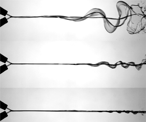
Figure 6. Lateral views of the sheet showing three wave profiles leading to flapping flag, sinuous and vibrating membrane instability, for (a)  $2\theta = 60^{\circ }$, (b) $2\theta = 90^{\circ }$ and (c) $2\theta = 120^{\circ }$. The vibrating membrane is a special case of sinuous instability in which the sheet is unaffected but a large section of the sheet surface shows very small-amplitude perturbations, similar to the vibrating thin membrane. The SPL level in all cases is 110 dB. See also supplementary movie 1, available at https://doi.org/10.1017/jfm.2021.251.
When the liquid sheet is perturbed at lower frequencies, the amplitude of the waves increases significantly and the sheet displays out-of-plane flapping. The wavelength of the waves is also relatively larger and the growth takes place within fewer wavelengths. Flapping of the liquid sheet similar to a flag was also observed in the case of a mechanically vibrated fan spray nozzle by Crapper et al. (Reference Crapper, Dombrowski, Jepson and Pyott1973). Hence, this type of breakup is termed the flapping flag type instability (named as flag in figure 6) to be consistent with the earlier works (Crapper et al. Reference Crapper, Dombrowski, Jepson and Pyott1973; Villermaux & Clanet Reference Villermaux and Clanet2002). In flapping flag type instability, the wave amplitudes grow monotonically over the entire sheet length, resulting in unbounded growth. This is also evident from the wave envelope corresponding to the flag type instability (figure 6) which shows the divergent pattern. This corresponds to a very high growth rate observed in the lower-frequency regime in figure 5. These growth rates exceed those predicted by the linear theories mainly because of the nonlinear effects resulting from the large and unbounded amplitudes.
Figure 6 also depicts the breakup of the liquid sheet in a pure sinuous mode (observed at moderate frequencies and shown in the second row) where both the sheet surfaces undulate in phase. Both the wavelength and the wave amplitude are seen to decrease and a relatively greater number of wavelengths appear on the sheet compared with the flag type. This is a result of reduced growth rate as compared to the flapping sheet. This kind of sheet breakup is dominated by the classical sinuous instability because the growth rate of sinuous waves is higher than the varicose mode (Squire Reference Squire1953). In the sinuous instability, the wave amplitudes are bounded as seen from the corresponding wave envelope. Hence, the growth rates in this frequency range match reasonably with the viscous linear stability predictions, as shown in figure 5.
For higher frequencies, the growth rate is observed to be still lower. The sheet mainly remains in its plane and the amplitude of the waves is not high enough to cause any change in the sheet characteristics. The visualization of such a sheet resembles a stretched membrane vibrating with high frequency but low amplitude. Hence, this type of sheet instability is termed the vibrating membrane type instability (as shown in figure 6). A vibrating membrane is a special case of sinuous mode in which the wave amplitudes saturate and are very small as compared to the sinuous type. It should be noted that all three instabilities evolve from the same sinuous perturbation introduced by the acoustics. However, their growth rates are so distinct that they result in completely different breakup characteristics. The sheet envelope for the vibrating membrane type breakup shows a very small growth rate, which is quite similar to that of the unperturbed sheet. However, it still has finite growth rate, which is comparable to the predictions of thinning theory. The frequency ranges in which these three distinct wave profiles are observed and their growth rate comparison with different theories are depicted in figure 5.
The high-frequency acoustics is unable to bring any noticeable change to the natural sheet breakup phenomenon. These forcing frequencies are higher than the lower cutoff frequency, as shown earlier in the work of Dighe & Gadgil (Reference Dighe and Gadgil2019a). This means that the breakup at forcing frequencies higher than the lower cutoff frequency is dictated by the vibrating membrane type breakup. For forcing frequencies smaller than the lower cutoff frequency, where the forcing brings appreciable changes to the sheet characteristics, the breakup may be dominated either by the flag type instability or by the sinuous wave instability. Both these modes belong to the unstable forcing condition, and the frequency separating these modes is termed here as the transition frequency ( $\,f_{t}$). In the following section, we try to establish the transition frequency based on experimental observations supported by certain theoretical measures.
3.3. Transition in instability patterns
The nature of waves and the associated features noticed for different types of instability patterns are significantly different. To derive the transition frequencies of the instability patterns objectively, the wave characteristics, such as the wave aspect ratio, the spatial wave growth and the critical length, are used. The wave aspect ratio ( $AR$) is defined as
 \begin{equation} AR = \frac{a_{m}}{\lambda}, \end{equation}
where  $a_{m}$ is the maximum wave amplitude and $\lambda$ is the wavelength.
Figure 7 shows the variation of the wave aspect ratio with forcing frequency for different Weber numbers (7a), and different SPLs (7b). It has been reported earlier by Villermaux & Clanet (Reference Villermaux and Clanet2002) that the wave aspect ratio remains almost constant (for their case,  $2a_{m}/\lambda \sim 0.8$) for naturally flapping liquid sheets. However, a close observation of figure 7(a) points out that, for a fixed Weber number and SPL, the aspect ratio is a non-monotonic function of forcing frequency. It initially increases with the increase in frequency, attains a peak value and decreases thereafter. A similar trend is observed for different Weber numbers. If the sheet breakup is governed by a unique mechanism at all forcing frequencies, then the wave aspect ratio is expected to be unaltered. Hence, we propose that this change in the variation of the aspect ratio is a consequence of the change in the growth pattern of instability. The forcing frequency at which the aspect ratio attains the maximum value for a given Weber number demarcates the shift from the flapping flag to the sinuous type of instability. Hence, this frequency is named the transition frequency ( $\,f_{t}$). The transition frequency increases with increase in the Weber number, as depicted by figure 7(a). The flag instability dominates for frequencies below the transition frequency, and the sinuous instability dominates for frequencies higher than the transition frequency. The transition frequencies for $We = 608$, 793 and 973 turn out to be 220, 320 and 420 Hz, respectively. The measured transition frequency values based on the aspect ratio are consistent with the observed breakup patterns (from lateral profiles of waves) for various frequencies.

Figure 7. Effect of forcing frequency on the wave aspect ratio, for  $2\theta = 90^{\circ }$. (a) Effect of Weber number on transition frequency. Here, $f_{1}$ is the first forcing frequency (100 Hz) and $f_{LC}$ is the lower cutoff frequency for $We = 793$. (b) Effect of SPL on transition frequency.
The trend presented in figure 7(b) corresponds to the same value of SPL. Figure 7(b) shows the typical effect of SPL on the transition frequency for  $We = 793$. It can be noted from figure 7(b) that the transition from flapping flag to sinuous instability (maximum value of the aspect ratio) occurs at nearly the same frequency. This indicates that the transition frequency is independent of the forcing amplitude and is a function of frequency only. Any generic instability evolution is also governed by the frequency rather than by the perturbation amplitude. Hence, it may be concluded that the aspect ratio variation is indeed a correct measure for identifying the transition frequency for flag to sinuous instabilities.
It is also interesting to note from figure 7(a) that there exists a particular frequency in the sinuous regime for each Weber number where the value of the aspect ratio falls below the value corresponding to the first forcing frequency ( $\,f_{1}$). These values of $AR$ tend to the $AR$ of the unexcited liquid sheet. The frequency after which the wave aspect ratio approaches the value of the unexcited condition interestingly matches with the lower cutoff frequency (as shown in figure 7(a) for $We = 793$), which is also an increasing function of Weber number. Hence, the lower cutoff frequency can be considered as the second transition frequency where the sheet breakup mechanism shifts from sinuous breakup to vibrating membrane type breakup.
3.4. Transition frequency based on the critical sheet length
It is clear from the previous analysis that the dominant instability mechanism responsible for sheet fragmentation is a function of forcing frequency. Here, the prediction of transition frequency in the context of the linear theory and its comparison with the experimentally observed transition frequency by wave aspect ratio is presented. When a flat liquid sheet is perturbed by the acoustic waves, the perturbation amplitude is proportional to the air particle displacement. The air particle displacement amplitude is extremely small and hence we use the linear stability theory for the predictions of transition frequency. The linear instability analysis conducted by Squire (Reference Squire1953) was used by Bremond et al. (Reference Bremond, Clanet and Villermaux2007) for analysis of an undulating circular sheet formed by jet impact on a mechanically vibrating circular cylinder, and later by Dighe & Gadgil (Reference Dighe and Gadgil2019a) for acoustically excited liquid sheets. In those studies, the concept of critical sheet length over which the sheet is unstable is employed. It is argued that the waves grow over this critical length, and beyond this critical length the growth ceases (Bremond et al. Reference Bremond, Clanet and Villermaux2007). Further, the critical sheet length ( $x_{c}$) over which the sheet is unstable is shown to be
 \begin{equation} \tilde{x}_{c}=\frac{W e}{1.4}\left(1-\left(\frac{\widetilde{\omega}_{0}} {\alpha W e}\right)^{1 / 2}\right). \end{equation}
 Here,  $\tilde {x}={x}/{d_{0}}$, $\widetilde {\omega }_{0}={2 {\rm \pi}f d_{0}}/{V}$ is the forcing frequency, $W e=\rho _{l} V^{2} d_{0} / \sigma$ is the Weber number of the liquid jet and $\alpha =\rho _{g} / \rho _{l}$. The critical sheet length (3.6) is a function of forcing frequency, Weber number and density ratio. Essentially, the critical sheet length signifies the length of the sheet over which the liquid sheet is unstable to the externally applied frequency.
A closer look at the sheet envelopes in the flag instability regime in figure 6 shows that the amplitudes grow monotonically till the sheet breaks up. Further evolution of the sheet envelope cannot be estimated, as the sheet breaks up, and hence it may be argued that the critical length is more than the sheet breakup length. If the sheet is assumed to be infinitely long, one may end up getting a sheet envelope similar to the sinuous mode of breakup where the spatial variation of amplitude is non-monotonic (grows and decays). The flag type of sheet envelope would evolve as shown in figure 8, if the sheet were infinitely long. The wave amplitude would diverge till the breakup point, reach a maximum value and decay further to form a closed envelope. The required sheet length to have such an imaginary envelope would be two times the sheet length till the breakup point. This gives us the criterion for the limiting value of the critical sheet length for flapping flag instability to sustain. Hence, it is proposed that, for the transition frequency below which only the flapping flag instability occurs, the critical sheet length should be equal to twice the sheet breakup length ( $x_{c}=2L$). From (3.6) and the transition frequency ( $\omega _{t} = 2 {\rm \pi}f_{t}$) criterion we have
 \begin{equation} \widetilde{\omega}_{t}=\alpha We\left(1-\frac{2.8 \widetilde{L}}{W e}\right)^{2}. \end{equation}
Figure 8. Schematic representation of critical sheet length. For the flag instability, the wave amplitude increases till sheet breakup. The solid line represents the sheet envelope.
Equation (3.7) signifies the frequency below which the flapping flag instability exists. The predicted transition frequency that demarcates the two instabilities is obtained from (3.7) for a given Weber number. Figure 9 shows the comparison between the transition frequency obtained experimentally and that predicted by the linear theory (3.7) for different Weber numbers. The predicted values of the transition frequencies are found to be in close agreement with the experimental measurements.

Figure 9. Transition frequencies separating the two instabilities as a function of Weber number.
The flapping or flag type instability was also observed earlier for a mechanically vibrated flat liquid sheet produced by fan spray nozzle (Crapper et al. Reference Crapper, Dombrowski, Jepson and Pyott1973, Reference Crapper, Dombrowski and Pyott1975), flat circular flapping sheets (Villermaux & Clanet Reference Villermaux and Clanet2002) and mechanically vibrated circular sheets formed by jet impact on a solid surface (Bremond et al. Reference Bremond, Clanet and Villermaux2007). In these previous studies, the flapping of the sheet is described as a sinuous flag-like instability. Although the flag type instability is an extreme case (ideally unbounded wave amplitudes) of the sinuous wave growth, the present study reveals that the flapping flag and the sinuous instabilities lead to completely distinct wave characteristics, and hence these are different types of sheet breakup mechanisms. These two instabilities are clearly evident in earlier works on mechanically vibrated fan spray nozzles reported by Crapper et al. (Reference Crapper, Dombrowski, Jepson and Pyott1973, Reference Crapper, Dombrowski and Pyott1975). Further, these similarities, independent of the type of perturbations (either acoustic or mechanical), illustrate the uniqueness in the response of the liquid sheet to the external perturbations.
3.5. Regimes of instability theories
It is clear from the literature as well as the above discussion that there are two major classes of theories which rely on different mechanisms of instability: (1) Squire's theory based on the aerodynamic interaction of the moving liquid sheet with the ambient gas, and (2) thinning theory based on the sheet thinning effect. We attempt to understand the relative dominance of both mechanisms and their relevance in the context of modelling the sheet instabilities in different frequency ranges. As the thinning theory is inviscid, the inviscid aerodynamic or Squire's theory has been employed for the instability mapping. A similar approach has also been adopted by Paramati et al. (Reference Paramati, Tirumkudulu and Schmid2015).
Paramati et al. (Reference Paramati, Tirumkudulu and Schmid2015) conducted the initial analysis of the effectiveness of the thinning theory in comparison with Squire's theory for a circular liquid sheet generated by the head-on collision of two liquid jets. Such types of liquid sheets produce the thickness distribution  $h = d_{0}^{2}/4x$. Some comparison with the liquid sheet produced by jet impact on a solid surface $h = d_{0}^{2}/8x$ (Bremond et al. Reference Bremond, Clanet and Villermaux2007) was also presented. For these cases, a regime map in Weber number–frequency ( $We$–
$We$– $\tilde {\omega }$) space was formulated to identify the conditions dominated by the respective effects. We observed that the features of this regime mapping are strongly governed by the thickness variation in the liquid sheets, and there was no conclusive study on this in the available literature. Hence, we obtain similar instability regime maps in $We$–
$We$– $\tilde {\omega }$ space for liquid sheets produced by varying the impingement angles. Impingement angles of $60^{\circ }$, $90^{\circ }$ and $120^{\circ }$ produce liquid sheets of different thickness distributions ( $h = d_{0}^{2}/0.287x$, $h = d_{0}^{2}/0.786x$ and $h = d_{0}^{2}/1.334x$, respectively) along the $\phi =0$ line. It is important to note that the local sheet thickness considered here represents much thicker liquid sheets than those of Paramati et al. (Reference Paramati, Tirumkudulu and Schmid2015) and Bremond et al. (Reference Bremond, Clanet and Villermaux2007) for similar jet diameters.
All these regime maps are shown in figure 10, which is qualitatively similar to figure 12 in Paramati et al. (Reference Paramati, Tirumkudulu and Schmid2015). The methodology and procedure for obtaining these regime maps is provided in Appendix C. The general features of this map are given here just for the sake of completeness. The regime map is obtained by comparing the growth rates predicted by both the theories. If a specific point on the map falls in the ‘thinning effect’ region, the growth rate predicted by the thinning theory exceeds that of Squire's theory for that particular combination of Weber number and frequency and vice versa. The dominant mechanism responsible for sheet fragmentation depends upon the combination of Weber number and frequency. There is a certain range of frequencies for a given Weber number in which the aerodynamic effects (Squire's theory) dominate, and this range of frequency increases with increase in Weber number. Below a specific Weber number, called the critical Weber number, the sheet breakup is solely governed by the thinning effect at all the forcing frequencies.

Figure 10. Regime maps showing the dominance of either the thinning effect or the aerodynamic plus thinning effect, for (a)  $2\theta = 60^{\circ }$, (b) $2\theta = 90^{\circ }$ and (c) $2\theta = 120^{\circ }$. The curve with circular markers separates the two regimes. (d) The cutoff frequencies using Squire's theory for a single jet impinging on a solid surface ( $h = d_{0}^{2}/8x$) (Bremond et al. Reference Bremond, Clanet and Villermaux2007) and the upper boundary of the envelope for a similar configuration (Paramati et al. Reference Paramati, Tirumkudulu and Schmid2015).
3.5.1. Effect of the sheet thickness
For each thickness distribution, we performed experiments at various Weber numbers and frequencies in order to study the sheet breakup over the whole map. These flow conditions are marked in figures 10(a), 10(b) and 10(c). The regime boundary in figure 10 represents the dividing line between two instability mechanisms where the growth rates predicted by the two mechanisms are equal. Figure 10(d) depicts a similar map for the experiments of Bremond et al. (Reference Bremond, Clanet and Villermaux2007). It may be seen from figure 10 that the critical Weber number (below which only the effect of sheet thinning dominates) increases as the liquid sheets become thinner. Consequently, the region of influence of the sheet thinning mechanism increases with the sheets becoming thinner. We present consolidated data of various liquid sheet configurations under external forcing that are analysed with the above two theories in table 1.
Table 1. Influence of sheet thickness variation on critical Weber number.
 $^{a}$This expression has been approximated to take a similar form to the other expressions for comparison purposes.
It may be inferred from table 1 that the critical value of the Weber number ( $We_c$) depends mainly on the sensitivity ( $\varepsilon$) of the sheet thickness with respect to the distance from the impact point (for the fan spray nozzle, $h = d_{0}^{2}/100x$ (an approximate expression as noted in the table)). To be specific, this scaling may be expressed as $We_{c} \sim \sqrt {\varepsilon }$. As the value of $\varepsilon$ increases for a given mass flow rate, the sheets become thinner progressively and the envelope of applicability of thinning theory increases. For example, the stability regime of the fan spray nozzle is mostly dictated by the thinning theory for all frequencies and practically all operating conditions (Majumdar & Tirumkudulu Reference Majumdar and Tirumkudulu2016). However, for thicker sheets ( $\varepsilon <1$), the critical $We$ becomes smaller and the dominating instability mechanism becomes a function of forcing frequency.
Another important observation can be drawn by plotting upper or higher cutoff frequencies (defined earlier in the work of Bremond et al. (Reference Bremond, Clanet and Villermaux2007) and Dighe & Gadgil (Reference Dighe and Gadgil2019a)) for respective maps in figure 10 (filled circles). The higher cutoff frequencies follow a similar trend to the upper branch of the regime boundary in all the cases. The higher cutoff frequency is a forcing frequency beyond which the spatial growth rate saturates and the sheet breakup is similar to that in the unexcited condition, with the most natural mode getting amplified (stable forcing condition (Bremond et al. Reference Bremond, Clanet and Villermaux2007)). The liquid sheet is practically unaffected by the external forcing with frequencies greater than the higher cutoff frequency. Hence, the prediction of the effect of external forcing becomes relevant when the forcing frequencies are lower than the higher cutoff frequency. The most notable aspect in the regime maps shown in figure 10 is the spacing between the higher cutoff frequency and the regime boundary. This spacing is also seen to be sensitive to the thickness distribution of the sheet. At lower impingement angle (or thicker sheets), the higher cutoff frequency is very close to the regime boundary for a given Weber number, as shown in figure 10(a). As the liquid sheet becomes thinner, the spacing between the higher cutoff frequencies and the regime boundary increases as shown in subsequent cases.
In the case of thicker sheets, the relevant forcing frequencies, which cause an appreciable rise in the growth rate, come inside the envelope of the aerodynamic effect. Squire's theory proposes that the aerodynamic interaction resulting from the relative velocity of the liquid sheet with respect to the ambient is responsible for the growth of the sinuous waves. Since the Weber number is an indication of the relative velocity, the range of frequencies over which Squire's theory dominates increases with Weber number in all the cases shown in figure 10(a). Hence, for predicting the effect of external forcing on thicker sheets, Squire's theory or aerodynamic interaction theory is more helpful. If the cases of relatively thinner sheets ( $\varepsilon >1$) are considered, like figures 10(c) and 10(d), there are a number of frequencies between the higher cutoff frequencies and the regime boundary in which the growth rates are better predicted considering the dominance of the sheet thinning effect. As the sheet becomes thinner, the range of forcing frequencies over which the thinning theory is reliable increases. Hence, the thinner sheets need both theories for predicting the effect of forcing over the range of relevant frequencies. Hence, it may be concluded that the thinner the liquid sheet, the larger will be the domain of influence of the sheet thinning theory.
3.5.2. Correlating the regime map with the experimental observations
Although the suitability of different instability formulations for different combinations of Weber number, forcing frequency and thickness distributions are proposed, it is also important to demonstrate the evolution of the instabilities dominated by different effects. This is particularly important in the context of the different wave growth profiles presented in § 3.2. It is clear from figure 10 that the aerodynamic interaction effect dominates at lower forcing frequencies while the thinning effect dominates at higher frequencies for a given Weber number (greater than the critical value). Two important profiles of the liquid sheet under forcing have been noticed in the previous analysis: large/moderate-amplitude flapping (flag and sinuous instability) of a liquid sheet at lower/moderate frequencies, and non-wavy, near-natural (vibrating membrane type breakup without significant growth rate) breakup at higher frequencies. These observations further indicate that sheet flapping or large amplification of sinuous waves is a characteristic feature resulting from the aerodynamic effect. The sheet thinning mechanism mainly results in vibrating membrane type of waves or natural breakup having relatively lower growth rates. These distinctions are particularly important in the context of the relatively thicker liquid sheets considered in the present study.
In view of this, we attempt to correlate the dominant sheet breakup mechanisms with the wave growth profiles. The experimental conditions for this illustration are chosen from the points marked in figure 10. Three different case studies are discussed to generalize the observations:
(i) for a fixed forcing frequency, varying the Weber number to traverse from the thinning region to the aerodynamic region;
(ii) effect of forcing frequencies at $We < We_{c}$ (belonging to the thinning region) for different thickness distributions; and
(iii) effect of forcing frequency at
$We > We_{c}$ by traversing from the aerodynamic region to the thinning region.


First, the sheet is excited with the same frequency and the region of dominance is changed from thinning alone to aerodynamic plus thinning by increasing the Weber number. The lateral sheet views shown in figure 11 correspond to  $\omega = 0.3$, $\textrm {SPL} = 110$ dB, $We = 130$ (thinning region on the envelope in figure 10a) and $We$ = 658 (aerodynamic plus thinning region on the envelope in figure 10a). Figures 11(a) and 11(b) show the instantaneous images of the liquid sheet under unexcited and excited conditions, respectively. It can easily be seen that external forcing does not bring any significant changes to the sheet structures (fluid chain type in this case) and both the sheet breakups (figures 11(a) and 11(b)) are almost the same. Also, the wavy pattern is not present in the forced breakup in figure 11(b). These are characteristic features of thinning-dominated breakup and may be observed in subsequent illustrations. It is also important to note that the breakup of the forced liquid sheet is similar to the natural breakup. The sheet structures in figures 11(c) and 11(d) are for unexcited and excited sheet breakup at higher Weber number that corresponds to the aerodynamic breakup regime. Whereas the unexcited sheet does not show any significant wavy structure, one may notice classical sinuous type instability and appreciable growth of wave amplitude in the case of external forcing.

Figure 11. Sheet excitation at the same frequency ( $\omega = 0.3$) but for different Weber numbers: (a,b) $2\theta = 60^{\circ }$, $We=130$, (a) unexcited case ( $\omega = 0$) and (b) $\omega = 0.3$, thinning region; (c,d) $2\theta = 60^{\circ }$, $We=658$, (c) unexcited case ( $\omega = 0$) and (d) $\omega = 0.3$, aerodynamic plus thinning region. Here $\textrm {SPL} = 110$ dB.
Now, we show different forcing conditions in the thinning region alone for different impingement conditions (having different thickness sensitivity). Side views of the liquid sheet in the thinning regime for Weber number less than the critical Weber number ( $We < We_{c}$) and different jet impingement angles ( $2\theta = 60^{\circ }$ and 120 $^{\circ }$) are shown in figure 12. For $2\theta = 60^{\circ }$, $We = 130$, figure 12(a) shows the unexcited sheet and figures 12(b) and 12(c) are with acoustic excitation at 120 Hz and 200 Hz, respectively. Sinuous waves are clearly absent on the sheet and there is no notable effect of acoustic field on the sheet structure. Similarly, figure 12(d) shows the natural sheet breakup for $We = 282$ and $2\theta = 120^{\circ }$. The effect of acoustic forcing with frequencies of 120 and 200 Hz is shown in figures 12(e) and 12(f), respectively. It may be noticed that the sheet breakup is similar to that of the natural breakup case. However, the sheet, being much thinner than the 60 $^{\circ }$ case, is getting displaced from its mean position due to the acoustic force without showing any growing wavy pattern.

Figure 12. Observed side views of the sheet in the thinning region alone: (a–c)  $2\theta = 60^{\circ }$, $We=130$, (a) unexcited case, (b,c) thinning region alone, (b) $We=130$, 120 Hz and (c) $We=130$, 200 Hz; (d–f) $2\theta =120^{\circ }$, $We=282$, (d) unexcited case, (e,f) thinning region alone, (e) $We=282$, 120 Hz and (f) $We=282$, 200 Hz. Here $\textrm {SPL} = 110$ dB.
Further, the cases with  $We > We_{c}$ are considered and the sheet is excited over a range of frequencies spanned over both regimes of influence, i.e. the aerodynamic plus thinning regime and the thinning regime. The sheet profiles for various thickness distributions are shown in figure 13. The top row indicates the sheet structures for $We = 658$, $2\theta = 60^{\circ }$. Figure 13(a) shows the natural breakup of the liquid sheet. Figures 13(b) and 13(c) show the sheet profiles for frequencies belonging to the aerodynamic region, and the sheet flapping is clearly observed. High forcing frequency conditions (thinning region) are shown in figures 13(d) and 13(e). It should be noticed that sheet waves are hardly visible and amplification is also less, which is similar to the case of natural breakup (figure 13a). A similar effect may be observed for thinner sheets with $We = 721$, $2\theta = 120^{\circ }$ in figure 13(f), unexcited, figures 13(g) and 13(h), acoustic forcing in the aerodynamic plus thinning region, and (figures 13(i) and 13(j)), the thinning region. Thus, these observations reinforce the relation between the mechanism of sheet breakup and the corresponding profiles of the interfacial waves.

Figure 13. Observed wave profiles in the aerodynamic plus thinning regime (ATR) and the thinning regime (TR) alone: (a)  $We=658$, unexcited; (b,c) ATR, (b) $We=658$, 100 Hz and (c) $We=658$, 120 Hz; (d,e) TR, (d) $We=658$, 620 Hz and (e) $We=658$, 680 Hz at 110 dB for $2\theta = 60^{\circ }$; (f) $We=721$, unexcited; (g,h) ATR, (g) $We=721$, 100 Hz and (h) $We=721$, 120 Hz; and (i,j) TR, (i) $We=721$, 680 Hz and (j) $We=721$, 700 Hz at 110 dB for $2\theta = 120^{\circ }$.
3.6. Discussion
It has been shown so far that there exist various types of sheet instability patterns and dominant breakup mechanisms which are dictated by the forcing frequency. If we collate all the understanding developed so far onto a single  $We$–
$We$– $\tilde {\omega }$ space, it will be definitely helpful to visualize the whole picture and assess the effects of forcing on the sheet breakup process. Such a plot for a liquid sheet (for $2\theta = 60^{\circ }$, i.e. $h = d_{0}^{2}/0.287x$) under the influence of acoustic forcing is shown in figure 14. Since the dominant sheet breakup mechanisms are sensitive to the thickness distribution, the plot shown in figure 14 changes as the sheet thickness distribution changes. However, the qualitative nature of the plot remains unaltered. There are two main regions: the aerodynamic plus thinning region and the thinning alone region shown on the regime map. The spatial wave growth rate comparison between the thinning theory and aerodynamic (Squire's) theory gives an envelope. Inside the envelope, aerodynamic plus thinning effects dominate, and only sheet thinning effects dominate in the outside region. This envelope is shown by the red curve in figure 14.

Figure 14. Region of influence of acoustic perturbations on the liquid sheet in Weber number versus frequency ( $We$–
$We$– $\tilde {\omega }$) space. The region of influence is a function of thickness sensitivity ( $\varepsilon$, with $h = d_{0}^{2}/\varepsilon x$) and changes accordingly with different impingement angles (which is shown earlier in figure 10); hence the envelope drawn here is, in general, shown without limits on the axes. The complete space is divided into two main regions: (I) the thinning region and (II) the aerodynamic plus thinning region. The envelope enclosed by the red line is dominated by the aerodynamic plus thinning effect, and outside this the thinning alone dominates. Significant changes in the sheet characteristics are observed within the red envelope only. The sheet shows three different breakup modes influenced by different instabilities: (A) flapping flag, (B-1) sinuous and (B-2) vibrating membrane instability (type of sinuous instability when forcing is stable). Corresponding sheet images and envelopes are also shown for $h = d_{0}^{2}/0.287x$. The curves shown by L-1, L-2 and L-3 are, respectively: transition (Squire's theory with thinning), lower cutoff (based on the sheet breakup length criterion) and upper cutoff (Squire's theory with thinning) frequencies that separate different modes of breakup.
The upper cutoff frequency obtained from the linear analysis is shown by the black line (L-3). The separation between line L-3 and the upper branch of the envelope (red line) is decided by the sheet thickness. The effect of acoustic perturbation on the liquid sheet ceases beyond the upper cutoff frequency and the liquid sheet behaves as if there were no external forcing. In the case of thinner liquid sheets, the region between line L-3 and the upper branch of the regime boundary is very crucial, as the sheet thinning theory is needed for the accurate prediction of instability characteristics. It should also be important to mention that the thinning theory is also better suited for the case of natural breakup. For thicker liquid sheets, most of the breakup dynamics can be predicted with the use of Squire's theory. Inside the red envelope, various effects of the acoustic perturbations on the liquid sheet starting from flapping flag to just vibrating like a thin membrane are observed. The violent flapping (A) motion is observed at lower frequencies below the transition frequency. Beyond the transition frequency to the lower cutoff frequency, the liquid sheet shows the sinuous (B-1) instability. These two wave profiles are characteristic features of the aerodynamic effect. The sheet shows the vibrating membrane type of instability (B-2) with further increase in the forcing frequency past the lower cutoff frequency. These three regimes are shown on the map as flapping flag, sinuous and vibrating membrane instabilities separated by the curves obtained by the transition (L-1) and lower cutoff (L-2) frequencies. The corresponding sheet lateral views and their phase-averaged envelopes (for  $2\theta = 60^{\circ }$, i.e. $h = d_{0}^{2}/0.287x$) demonstrating three instability patterns are also shown in figure 14.
It is important to note at this point that a similar type of vibrating membrane instability spans across the boundary of the regime envelope. As mentioned earlier, the regime boundary is the frequency at which the growth rate predicted by the inviscid thinning theory exceeds that of the inviscid aerodynamic theory. Since both the inviscid theories provide dispersion relations to enable us to arrive at the regime map with ease, inviscid formulations are used in the existing work. However, a closer look at figure 3 indicates that the growth rate predicted by the thinning theory exceeds that of the viscous theory at a much lower frequency than the inviscid theory. Had the viscous theory been used to obtain the regime map, the regime boundary must appear in the vicinity of the lower cutoff frequencies. In that scenario, the complete region of the vibrating membrane type of instability would belong to the thinning theory zone. It should also be noted that all the transition frequencies and the cutoff frequencies can be well predicted by the use of the linear theory. Below the critical Weber number, the transitions are not noticed, as the sheet breakup is solely governed by the thinning effect. If the liquid sheet geometry (thickness distribution), the range of Weber numbers and the forcing frequencies are known, then figure 14 serves as a guideline for determining the qualitative sheet behaviour, the most appropriate modelling approach and various transition frequencies influencing the atomization characteristics.
4. Conclusion
Experimental investigations on the effect of external acoustic forcing on the evolution of liquid sheet instabilities have been carried out. By varying the acoustic wave frequency and the injection conditions, we have demonstrated the existence of three distinct patterns of the growth of instability waves. At lower forcing frequencies, the sheet displays flag-like flapping in which the wave amplitude diverges till the breakup point and the wave profile is highly non-sinusoidal. The second type is the classical sinuous instability, in which the wave amplitude grows in a bounded fashion before the sheet breaks and the wave profile remains sinusoidal. At higher forcing frequencies, the third type of instability pattern, called a vibrating membrane, is observed and the wave growth rate is seen to saturate to that of the natural breakup. Although all the instability patterns result from the sinuous perturbations, their instability features, like wave aspect ratio and spatial growth rate, are clearly distinctive. It is shown that the instability patterns are a function of forcing frequency. The transition frequency and the lower cutoff frequency demarcate the flapping flag to sinuous and the sinuous to vibrating membrane instability transitions, respectively. It is found that the transition frequency can be well predicted by using the linear instability theory.
Further, the experimentally measured instability characteristics are assessed with the help of existing instability theories. According to two established theories, the primary effects, which dominate the sheet breakup, are its aerodynamic interaction (Squire's theory (Squire Reference Squire1953)) and the sheet thinning effect (Tirumkudulu & Paramati Reference Tirumkudulu and Paramati2013). In order to determine the regime of applicability of each theory, the response to acoustic forcing of liquid sheets having different thickness distributions is evaluated. By combining the measurements of the present work and trends reported in the literature, it is shown that the sheet thickness primarily determines the dominant mechanism that governs the breakup. Based on the stability calculations, an instability regime map is formulated in  $We$–
$We$– $\tilde {\omega }$ space. It may be noted, in general, that the aerodynamic interaction mechanism is dominant at lower forcing frequencies and the sheet thinning effect takes over at higher frequencies. The change-over frequency is in the vicinity of the upper cutoff frequency, and the separation between these two increases as the sheet becomes thinner. Hence, it is proposed that Squire's theory is more useful for thicker sheets in the frequency domain where the forcing augments the growth rate of the instability. The thinning theory performs well over a wider range of frequencies in the case of thinner sheets as well as natural breakup events. These conclusions are confirmed with the help of visualizations of the instability patterns where the breakup dominated by each effect shows distinct wave structure. Finally, a universal regime map is proposed to enable the choice of the right theoretical formulation for predicting the sheet stability characteristics.
Supplementary movie
A supplementary movie is available at https://doi.org/10.1017/jfm.2021.251.
Acknowledgements
The authors acknowledge financial assistance from the Indian Institute of Technology Bombay.
Funding
This work was supported by the Indian Institute of Technology Bombay, grant number 15IRCCSG008.
Declaration of interests
The authors report no conflict of interest.
Appendix A. Measurement of the experimental growth rate
The wave amplitude growth on the liquid sheet is visualized using shadowgraphy of the side views of the liquid sheet. Although the growth rate should be measured near the impingement location, to be consistent with linear stability, it is evident from the sheet envelopes in figure 6 that the wave amplitudes near the impingement point are very low. Reliable measurements near the impingement point are hence not possible due to the limitation of the optical resolution.
Thus the measurement of the location of maximum wave amplitude is carried out from a single image (out of 500 images) having maximum wave amplitude. The experimental growth rate is calculated from the maximum wave amplitude and its location downstream of the impingement point using (3.2). A similar approach was adapted by Crapper et al. (Reference Crapper, Dombrowski and Pyott1975). It is known that the growth rate is an exponent and it is also evident from figure 15 that the growth rates for all three instability patterns are indeed exponential. However, the experimental estimation of growth rate is done using an inverse tan function (3.2) for the following reasons:
(i) In linear stability analysis, the growth rates are derived with the assumption that the initial perturbation is independent of the forcing frequency. However, in the present case, the initial acoustic perturbation is a strong function of acoustic frequency (
$a_{0} \propto \omega ^{-2}$) for a constant SPL.(ii) In linear theory, the growth rate is a function of forcing frequency (stability curve from figure 3) since the initial perturbation is not a function of frequency. If the conventional formulation for growth rate determination (
$\beta =x_{1}^{-1} \ln ({a_{m}}/{a_{0}})$) is used, the frequency dependence of the growth rate gets neutralized, as seen from the nearly constant slopes of the curves in figure 15. Physically, the measurements show that both the maximum wave amplitude and the perturbation amplitude decay with increase in the frequency, leading to a constant growth rate over the complete range of forcing frequencies. However, the flow visualizations show significant variations in the spatial growth rates with frequency. The nearly constant growth rate prediction by the conventional exponent method does not give a realistic depiction of this phenomenon.(iii) In order to get frequency-dependent growth rates, the perturbation amplitude is not employed in the growth rate estimation. The growth rate is assumed to be a function of the maximum wave amplitude and its location from the impingement point. Use of the inverse tan function gives the non-dimensional measure of the growth rate to compare with the predictions of different theories. It should further be noted that this method of growth rate estimation gives clear distinctions between different instability patterns based on the theoretical comparisons. It is also important to understand that the present method for growth rate measurement is not generic and may be used when the forcing frequency and the amplitude are strongly coupled.


Figure 15. Spatial amplitude growth ( $2\theta = 60^{\circ }$, $We = 658$, 110 dB) for flapping flag (120 Hz), sinuous (260 Hz) and vibrating membrane type (460 Hz). Here $a_{0}$ is the initial perturbation amplitude given by the acoustic source.
Appendix B. Growth rate prediction for viscous case
It is known that the viscous boundary layer at the liquid–air interface influences the spatial growth of the wave. The effect of boundary layer formation on the spatial wave growth is investigated using linear theory. In the present analysis, we have employed the spectral collocation method, which has been adapted by many researches for the growth rate prediction for a viscous liquid sheet and viscous gas (Söderberg & Alfredsson Reference Söderberg and Alfredsson1998; Söderberg Reference Söderberg2003; Tammisola et al. Reference Tammisola, Sasaki, Lundell, Matsubara and Söderberg2011; Ye et al. Reference Ye, Yang and Fu2016). To predict the spatial growth rate, we used the MATLAB tool ‘Hydrostab’ recently developed by Ye et al. (Reference Ye, Yang and Fu2016). Details of this method with a sample code can be found in Ye et al. (Reference Ye, Yang and Fu2016). The liquid sheet thickness in the viscous analysis is taken to be constant and calculated from the expression given by Miller (Reference Miller1960). Note that the growth rate prediction using the viscous theory is carried out at the location of maximum wave amplitude. The liquid sheet thickness just below the impingement point (at 0.03 mm on the  $\phi = 0$ line) is obtained from the thickness distribution formula (Miller Reference Miller1960) and this thickness is assumed constant for the prediction of the growth rate. Here, we have provided the governing equations, the boundary conditions and the gas velocity profile used in the current analysis. For consistency, these equations are presented in a similar way as given in Ye et al. (Reference Ye, Yang and Fu2016). We consider the liquid sheet as shown in figure 2 with viscous liquid and viscous surrounding gas.
B.1. The governing equations
For layer 1 ( $-h / 2 < y < h / 2$),
 \begin{gather} \frac{\partial u_{1}}{\partial x}+\frac{\partial v_{1}}{\partial y}=0, \end{gather}
 \begin{gather}\rho_{l}\left(\frac{\partial u_{1}}{\partial t}+u \frac{\partial u_{1}}{\partial x}\right)={-}\frac{\partial p_{1}}{\partial x}+\mu_{l}\left(\frac{\partial^{2} u_{1}}{\partial x^{2}}+\frac{\partial^{2} u_{1}}{\partial y^{2}}\right), \end{gather}
 \begin{gather}\rho_{l}\left(\frac{\partial v_{1}}{\partial t}+u \frac{\partial v_{1}}{\partial x}\right)={-}\frac{\partial p_{1}}{\partial y}+\mu_{l}\left(\frac{\partial^{2} v_{1}}{\partial x^{2}}+\frac{\partial^{2} v_{1}}{\partial y^{2}}\right). \end{gather}
For layer 2 ( $y>h / 2$),
 \begin{gather} \frac{\partial u_{g 2}}{\partial x}+\frac{\partial v_{g 2}}{\partial y}=0, \end{gather}
 \begin{gather}\rho_{g}\left(\frac{\partial u_{g 2}}{\partial t}+U_{g} \frac{\partial u_{g 2}}{\partial x}+v_{g 2} \frac{\partial U_{g 2}}{\partial y}\right)={-}\frac{\partial p_{g 2}}{\partial x}+\mu_{g}\left(\frac{\partial^{2} u_{g 2}}{\partial x^{2}}+\frac{\partial^{2} u_{g 2}}{\partial y^{2}}\right), \end{gather}
 \begin{gather}\rho_{g}\left(\frac{\partial v_{g 2}}{\partial t}+U_{g 2} \frac{\partial v_{g 2}}{\partial x}\right)={-}\frac{\partial p_{g 2}}{\partial y}+\mu_{g}\left(\frac{\partial^{2} v_{g 2}}{\partial x^{2}}+\frac{\partial^{2} v_{g 2}}{\partial y^{2}}\right). \end{gather}
For layer 3 ( $y<-h / 2$),
 \begin{gather} \frac{\partial u_{g3}}{\partial x}+\frac{\partial v_{g3}}{\partial y}=0, \end{gather}
 \begin{gather}\rho_{g}\left(\frac{\partial u_{g 3}}{\partial t}+U_{g} \frac{\partial u_{g 3}}{\partial x}+v_{g 3} \frac{\partial U_{g}}{\partial y}\right)={-}\frac{\partial p_{g 3}}{\partial x}+\mu_{g}\left(\frac{\partial^{2} u_{g 3}}{\partial x^{2}}+\frac{\partial^{2} u_{g 3}}{\partial y^{2}}\right), \end{gather}
 \begin{gather}\rho_{g}\left(\frac{\partial v_{g 3}}{\partial t}+U_{g} \frac{\partial v_{g 3}}{\partial x}\right)={-}\frac{\partial p_{g 3}}{\partial y}+\mu_{g}\left(\frac{\partial^{2} v_{g 3}}{\partial x^{2}}+\frac{\partial^{2} v_{g 3}}{\partial y^{2}}\right). \end{gather}
B.2. Boundary conditions
B.2.1. The kinematic boundary conditions
At the top interface ( $y=h / 2$),
 \begin{gather} v_{1}=\frac{\partial \eta_{1}}{\partial t}+u \frac{\partial \eta_{1}}{\partial x}, \end{gather}
 \begin{gather}v_{g2}=\frac{\partial \eta_{1}}{\partial t}+U_{g} \frac{\partial \eta_{1}}{\partial x}, \end{gather}
 \begin{gather}u_{1}=u_{g2}+\eta_{1} \frac{\partial U_{g}}{\partial y}. \end{gather}
At the bottom interface ( $y=-h / 2$),
 \begin{gather} v_{1}=\frac{\partial \eta_{2}}{\partial t}+u \frac{\partial \eta_{2}}{\partial x}, \end{gather}
 \begin{gather}v_{g3}=\frac{\partial \eta_{2}}{\partial t}+U_{g} \frac{\partial \eta_{2}}{\partial x}, \end{gather}
 \begin{gather}u_{1}=u_{g3}+\eta_{2} \frac{\partial U_{g}}{\partial y}. \end{gather}
B.2.2. The dynamic boundary conditions
At the top interface ( $y=h / 2$),
 \begin{gather} \mu_{l}\left(\frac{\partial u_{1}}{\partial y}+\frac{\partial v_{1}}{\partial x}+ \frac{\partial^{2} u}{\partial y^{2}}\eta_{1}\right)=\mu_{g}\left(\frac{\partial u_{g2}}{\partial y}+\frac{\partial v_{g2}}{\partial x}+\frac{\partial^{2} U_{g}}{\partial y^{2}}\eta_{1} \right), \end{gather}
 \begin{gather}p_{1}-2 \mu_{l} \frac{\partial v_{1}}{\partial y}-p_{g2}+2 \mu_{g} \frac{\partial v_{g2}}{\partial y}={-}\sigma \frac{\partial^{2} \eta_{1}}{\partial x^{2}}. \end{gather}
At the bottom interface ( $y=-h / 2$),
 \begin{gather} \mu_{g}\left(\frac{\partial u_{g3}}{\partial y}+\frac{\partial v_{g3}}{\partial x}+ \frac{\partial^{2} U_{g}}{\partial y^{2}}\eta_{2}\right)=\mu_{l}\left(\frac{\partial u_{1}}{\partial y}+\frac{\partial v_{1}}{\partial x}+\frac{\partial^{2} u}{\partial y^{2}}\eta_{2} \right), \end{gather}
 \begin{gather}p_{g3}-2 \mu_{g} \frac{\partial v_{g3}}{\partial y}-p_{1}+2 \mu_{l} \frac{\partial v_{1}}{\partial y}={-}\sigma \frac{\partial^{2} \eta_{2}}{\partial x^{2}}. \end{gather}
B.3. Gas velocity profile
To obtain the spatial growth rate in the viscous case, the gas motion can be described by various models. Here, the gas velocity profile given by the modified Stokes boundary layer (Schlichting Reference SavartReference SavartReference Schlichting1979) is employed, since it has been shown that the experimental growth rates can be well predicted by the modified Stokes boundary layer model (Söderberg & Alfredsson Reference Söderberg and Alfredsson1998; Söderberg Reference Söderberg2003; Tammisola et al. Reference Tammisola, Sasaki, Lundell, Matsubara and Söderberg2011; Ye et al. Reference Ye, Yang and Fu2016). Hence, in the present analysis, we choose the following gas velocity profile given by the modified Stokes model:
 \begin{equation} U_{g}(X, y)=u\left(X, \pm \frac{h}{2}\right)(1- \textrm{erf}(\eta)), \quad \eta=(|y|-1)\left(\sqrt{\frac{u \rho_{g}}{\mu_{g} X}}\right). \end{equation}
Appendix C. Methodology of obtaining the regime map
The regime map splits the region of influence of the thinning effect and the aerodynamic effect in the Weber number versus frequency space ( $We$–
$We$– $\tilde {\omega }$). These maps are obtained by comparing the spatial growth rate of waves calculated by using the thinning and aerodynamic plus thinning theories over the length of the sheet. This procedure is adopted from the work of Tirumkudulu & Paramati (Reference Tirumkudulu and Paramati2013) and given here for the sake of completeness.
Figure 16(a) shows the predicted growth rate as a function of spatial location on the sheet axis obtained by solving (3.1) and (3.4). The spatial growth rates predicted by thinning alone diverge at the point of impingement and the sheet edge. It may be clear from figure 16(a) that the growth rate is a function of forcing frequency. Depending on the forcing condition, the growth rate either by the thinning theory or by the aerodynamic theory dominates over the major portion of the sheet. Either at very low or at very high frequencies the growth rate predicted by the aerodynamic theory is less than the thinning theory. Hence, for a fixed Weber number, there exists two frequencies at which the growth rate by the aerodynamic theory and by the thinning theory are equal. For example, for  $We=302$, $f=8$ Hz and $f = 114$ Hz the growth rates are equal at non-dimensional spatial locations of 0.15 and 0.50, as shown in figure 16(a). The growth rate predicted by the aerodynamic theory dominates over a range of frequencies that are in between these (8–114 Hz) two frequencies. If the forcing is outside this range ( $\textrm {frequencies}<8$ Hz and $\textrm {frequencies}>114$ Hz), the growth rate predicted by the thinning theory dominates. For each Weber number these two frequencies can be calculated from the growth rate comparison as explained earlier, and from these measurements the regime map showing the dominance of the thinning and aerodynamic theory in $We$–
$We$– $\tilde {\omega }$ space can be obtained. Such a regime map for $2\theta = 90^{\circ }$ and $h = d_0^2/0.686x$ is shown in figure 16(b). The regime map shown in figures 10(a), 10(b) and 10(c) are obtained by a similar procedure.

Figure 16. (a) Predicted growth rate by Squire's theory (aerodynamic) and thinning theory as a function of distance on the sheet axis for  $We=302$, and $f = 1$, 8, 25 114 and 140 Hz. (b) Regime map showing the dominance of either thinning or aerodynamic plus thinning effect. The dotted line separates the two regimes.


 Open access