


1. Introduction
When an acoustic field encounters inhomogeneity, it exerts acoustic radiation force on it. Here, by inhomogeneity, we mean non-uniform or discontinuous variation of physical properties in a system such as particles/cells suspended in fluid, emulsions, co-flowing streams of miscible or immiscible fluids, and fluid subjected to a temperature gradient. The acoustic forces acting on inhomogeneity are extensively studied in microscale flows, and this field is known as ‘microscale acoustofluidics’ (Friend & Yeo Reference Friend and Yeo2011). Over the last two decades, acoustofluidics has found a wide range of applications in biological (Christakou et al. Reference Christakou, Ohlin, Vanherberghen, Khorshidi, Kadri, Frisk, Wiklund and Önfelt2013; Collins et al. Reference Collins, Morahan, Garcia-Bustos, Doerig, Plebanski and Neild2015; Iranmanesh et al. Reference Iranmanesh, Ramachandraiah, Russom and Wiklund2015; Ahmed et al. Reference Ahmed, Ozcelik, Bojanala, Nama, Upadhyay, Chen, Hanna-Rose and Huang2016; Lakshmanan et al. Reference Lakshmanan, Jin, Nety, Sawyer, Lee-Gosselin, Malounda, Swift, Maresca and Shapiro2020), chemical (Shi et al. Reference Shi, Huang, Stratton, Huang and Huang2009; Xie et al. Reference Xie, Rufo, Zhong, Rich, Li, Leong and Huang2020) and medical (Li et al. Reference Li2015; Lu et al. Reference Lu, Martin, Soto, Angsantikul, Li, Chen, Liang, Hu, Zhang and Wang2019; Zhang et al. Reference Zhang, Tian, Bachman, Zhang and Huang2020) sciences.
Recently, the relocation and stabilization of inhomogeneous co-flowing fluid streams in microchannels have gained the attention of the research community which is evident from the following works. Through silicon-glass microchannel experiments, using standing bulk acoustic waves, Deshmukh et al. (Reference Deshmukh, Brzozka, Laurell and Augustsson2014) could relocate the high-impedance sodium chloride solution to the pressure node (centre) and the low-impedance water to the pressure anti-node (sides). Also, they could stabilize a high-impedance fluid at the centre (and the low-impedance fluid to the sides) against gravity stratification using acoustic fields. Following this, using the hypothesis on mean Eulerian pressure, Karlsen, Augustsson & Bruus (Reference Karlsen, Augustsson and Bruus2016) derived the acoustic body force to explain the relocation of inhomogeneous fluids. Using the same theory, Karlsen et al. (Reference Karlsen, Qiu, Augustsson and Bruus2018) showed that the acoustic body force acting on stable inhomogeneous fluid configuration could effectively suppress the boundary-driven Rayleigh streaming in the bulk. In addition to the above works on inhomogeneous miscible fluids, Hemachandran et al. (Reference Hemachandran, Karthick, Laurell and Sen2019) experimentally demonstrated the relocation of immiscible fluids using acoustic fields by overcoming the interfacial tension forces. Hoque & Sen (Reference Hoque and Sen2023) extended the analysis on immiscible fluids to study the dependence on the speed of sound, density of the fluid and the width of the fluid stream on frequency. They showed that a single resonant frequency can be achieved for the co-flowing fluids for a given width ratio. Other notable works on the practical applications of acoustic forces on co-flowing inhomogeneous fluids include iso-acoustic focusing of cells (Augustsson et al. Reference Augustsson, Karlsen, Su, Bruus and Voldman2016), acoustic focusing of sub-micron particles (Gautam et al. Reference Gautam, Gurung, Fencl and Piyasena2018; Van Assche et al. Reference Van Assche, Reithuber, Qiu, Laurell, Henriques-Normark, Mellroth, Ohlsson and Augustsson2020), tweezing and patterning of inhomogeneous fluids in a microchannel (Karlsen & Bruus Reference Karlsen and Bruus2017; Baudoin et al. Reference Baudoin, Thomas, Al Sahely, Gerbedoen, Gong, Sivery, Matar, Smagin, Favreau and Vlandas2020), rapid mixing of fluids using an alternating multinode method (Pothuri, Azharudeen & Subramani Reference Pothuri, Azharudeen and Subramani2019), and reversible stream–droplet transition in a microfluidic co-flowing immiscible system (Hemachandran et al. Reference Hemachandran, Hoque, Laurell and Sen2021).
In our previous work (Rajendran et al. Reference Rajendran, Jayakumar, Azharudeen and Subramani2022), the theory of acoustic forces acting on inhomogeneous fluids was developed from first principles, without any prior assumptions on the mean Eulerian pressure. The generalized acoustic body force derived was shown to predict the experimental results of Deshmukh et al. (Reference Deshmukh, Brzozka, Laurell and Augustsson2014), Karlsen et al. (Reference Karlsen, Augustsson and Bruus2016), Karlsen et al. (Reference Karlsen, Qiu, Augustsson and Bruus2018) and Hemachandran et al. (Reference Hemachandran, Karthick, Laurell and Sen2019). It was proved that an impedance gradient is a necessary condition for the relocation/stabilization of inhomogeneous fluids under acoustic fields. Nevertheless, due to the intricacy of the acoustic body force equation, the stability of a particular configuration cannot be readily inferred from it without performing numerical simulations. Although the relocation force component from the generalized acoustic body force is deduced by Rajendran et al. (Reference Rajendran, Jayakumar, Azharudeen and Subramani2022), the exact conditions at which an inhomogeneous system relocates, remains stable or is neutral are not established. To address the above problem, this paper aims to provide the stability criterion (a simple algebraic equation) from which one can obtain a complete and clear picture of the stability of inhomogeneous fluids subjected to acoustic fields.
In this work, using linear stability analysis, we derive the characteristic equation that governs the stability of inhomogeneous fluids (with and without interfacial tension) under an acoustic body force. We study the various parameters such as the initial arrangement of fluids, the position of the interface with respect to the pressure node and pressure antinodes, acoustic energy density, the height of the channel or fluid interface, and surface tension to establish the necessary and sufficient conditions for relocation and stability. For fluids with interfacial tension, a non-dimensional number called the acoustic Bond number is obtained theoretically which characterizes the stable and unstable (relocation) regimes. Also, we deduce a relation between the critical acoustic energy density and the height of the channel which paves a way for relocating fluids with higher interfacial tension  $(O(10^1\ {\rm mN}\ {\rm m}^{-1}$ to $10^2\ {\rm mN}\ {\rm m}^{-1}))$ in a microchannel. Furthermore, numerical simulations are carried out using a generalized acoustic body force which agrees well with the derived theoretical stability criterion.
2. Physics of the problem
The hydrodynamics of the inhomogeneous fluids involved in this study is governed by the mass-continuity and momentum equations (Landau & Lifshitz Reference Landau and Lifshitz1987),
 $$\begin{gather} \frac{\partial\rho}{\partial t}+\boldsymbol{\nabla}\boldsymbol{\cdot}(\rho {\boldsymbol{V}})=0, \end{gather}$$
 $$\begin{gather}\rho \frac{{\rm D}{\boldsymbol{V}}}{{\rm D}t}=-\boldsymbol{\nabla} p +\eta\nabla^2 {\boldsymbol{V}} +\beta\eta\boldsymbol{\nabla}(\boldsymbol{\nabla}\boldsymbol{\cdot}{\boldsymbol{V}}) + {\boldsymbol{f}}_{ac}, \end{gather}$$
where  $\rho$ represents density, ${\boldsymbol {V}}$ represents the velocity vector field, $p$ represents the pressure field, $\eta$ is the dynamic viscosity of the fluid, $\beta =(\xi /\eta )+(1/3)$, $\xi$ is the bulk viscosity, ${\rm D}/{\rm D}t$ denotes the material derivative ( ${\rm D}/{\rm D}t=\partial _t+{\boldsymbol {V}}\boldsymbol {\cdot }\boldsymbol {\nabla }$) and all the above fields vary at a slow time scale $t$.
$t$.
The body force  ${\boldsymbol {f}}_{ac}$ responsible for the above slow time scale phenomena is created by the acoustic fields varying at a fast time scale ( $t_f$). In general, the dependent fields such as velocity, pressure, density and compressibility can be decomposed using perturbation theory, based on the time scales as $g_\tau =g(\boldsymbol {r},t)+g_1(\boldsymbol {r},t_f)$, where $g_1(\boldsymbol {r},t_f) = g_1(\boldsymbol {r}) {\rm e}^{-{\rm i}\omega t_f}$ is a first-order time-harmonic acoustic field that varies on the fast time scale $t_f\ (t_f \sim 1/\omega \sim 0.1\ \mathrm {\mu } {\rm s})$, $\omega ({\sim }1\ {\rm MHz})$ is the angular frequency of the acoustic fields and $g$ is the fields that vary on a slow time scale $t (t \gg t_f)$. The slow time scale phenomena such as acoustic streaming, acoustic relocation and streaming suppression are created by ${\boldsymbol {f}}_{ac}$ which is the divergence of the time-averaged Reynolds stress tensor consisting of the product of first-order fast time scale acoustic fields (Rajendran et al. Reference Rajendran, Jayakumar, Azharudeen and Subramani2022),
 \begin{align} {\boldsymbol{f}}_{ac}
=-\boldsymbol{\nabla}\boldsymbol{\cdot}\langle\rho{\boldsymbol{v}}_1
{\boldsymbol{v}}_1\rangle &= \left(
\tfrac{1}{2}\boldsymbol{\nabla} (\kappa\langle|p_1|^2\rangle - \rho
\langle|{\boldsymbol{v}}_1|^2\rangle)\right) +
\left(\langle{\boldsymbol{v}}_1\times\boldsymbol{\nabla}\times(\rho{\boldsymbol{v}}_1)\rangle\right)
\nonumber\\ &\quad +
\left(-\tfrac{1}{2}\langle|p_1|^2\rangle\boldsymbol{\nabla}\kappa-\tfrac{1}{2}\langle{\boldsymbol{v}}_1^2\rangle\boldsymbol{\nabla}\rho\right)
\end{align}
\begin{align} {\boldsymbol{f}}_{ac}
=-\boldsymbol{\nabla}\boldsymbol{\cdot}\langle\rho{\boldsymbol{v}}_1
{\boldsymbol{v}}_1\rangle &= \left(
\tfrac{1}{2}\boldsymbol{\nabla} (\kappa\langle|p_1|^2\rangle - \rho
\langle|{\boldsymbol{v}}_1|^2\rangle)\right) +
\left(\langle{\boldsymbol{v}}_1\times\boldsymbol{\nabla}\times(\rho{\boldsymbol{v}}_1)\rangle\right)
\nonumber\\ &\quad +
\left(-\tfrac{1}{2}\langle|p_1|^2\rangle\boldsymbol{\nabla}\kappa-\tfrac{1}{2}\langle{\boldsymbol{v}}_1^2\rangle\boldsymbol{\nabla}\rho\right)
\end{align}
 \begin{align} &= (\,{\boldsymbol{f}}_{{ac}_1})+(\,{\boldsymbol{f}}_{{ac}_2})+(\,{\boldsymbol{f}}_{{ac}_3}), \end{align}
where  $p_1$ and ${\boldsymbol {v}}_1$ denote the first-order (fast time scale) pressure and velocity fields due to acoustic waves (see Appendix A) and $\langle \cdots \rangle$ indicates time averaging over a period $t \gg t_f$ (the time average of two first-order fields $\langle {\boldsymbol {u}}_1{\boldsymbol {v}}_1\rangle$ is defined as $\frac {1}{2}{\rm Re}({\boldsymbol {u}}_1^{\star }{\boldsymbol {v}}_1$), where $\star$ denotes complex conjugation). The terms $\rho$ and $\kappa$ denote the slow time scale (background) density and compressibility of the fluid respectively. In (2.2), the first term $({\boldsymbol {f}}_{{ac}_1})$ is a conservative or gradient term that induces pressure and not fluid flow, the second term $({\boldsymbol {f}}_{{ac}_2})$ is only dominant at boundary layers and is responsible for boundary-driven Rayleigh streaming, and the third term $({\boldsymbol {f}}_{{ac}_3})$ is responsible for relocation and stabilization of inhomogeneous fluids. Hence, only the relevant third term, ${\boldsymbol {f}}_{{ac}_{3}}$, is considered for theoretical analysis. For the standing acoustic wave applied along the $x$-direction, the pressure $p_1=p_a\sin (k_wx)$ and velocity ${\boldsymbol {v}}_1=(\,p_a/i\rho c)\cos (k_wx)$, where $p_a$ denotes the pressure amplitude, $c$ denotes the speed of sound in a medium, $k_w = 2{\rm \pi} /\lambda _w$ denotes the wavenumber, $\lambda _w$ denotes the wavelength (for standing half-wave, $\lambda _w = 2w$, where $w$ is the width of the channel). The force term ${\boldsymbol {f}}_{rl}$ causing the relocation can be obtained from ${\boldsymbol {f}}_{{ac}_{3}}$ after disregarding the conservative term, which can be written as (Rajendran et al. Reference Rajendran, Jayakumar, Azharudeen and Subramani2022)
 \begin{equation} {\boldsymbol{f}}_{rl}=-E_{ac}\cos({2k_wx})\boldsymbol{\nabla}\tilde{Z}, \end{equation}
where  $E_{ac}=p_a^2/(4\rho _{avg}c_{avg}^2)=(v_a^2\rho _{avg})/4$ is the acoustic energy density, $v_a$ denotes the velocity amplitude, $Z = \rho c$ denotes impedance, $\tilde {Z}=Z/Z_{avg}$, $\tilde {c} = c/ c_{avg}$ and $\tilde {\rho } = \rho / \rho _{avg}$, where the subscript ‘avg’ denotes the respective average quantities of fluids $A$ and $B$. Here, $x=0$ denotes the pressure node and $x=\pm w/2$ denote the pressure anti-nodes. To improve readability, throughout the manuscript, ‘pressure node’ and ‘pressure anti-nodes’ are referred to as ‘node’ and ‘anti-node’ respectively. It is important to note that the first-order fields $p_1$ and $v_1$ assumed for the theoretical analysis correspond to a homogeneous fluid. However, an inhomogeneous fluid configuration of different fluid impedances ( $Z_A$ and $Z_B$) leads to different pressure fields and different acoustic wavelengths in the two fluids. The accuracy of this assumption is evaluated using numerical simulations in § 3.2, where the variation of the pressure field in each fluid is taken into account.
2.1. Stability analysis of inhomogeneous fluids in the absence of interfacial tension
A two-dimensional fluid domain subjected to a standing acoustic half-wave in the  $x$-direction, with two fluids separated by a sharp vertical interface, as shown in figure 1(a–c), is considered for the stability analysis. Before beginning the analysis, it is necessary to understand the equilibrium of the system in the absence of interfacial tension. In a completely enclosed domain, a fluid initially at rest ( ${\boldsymbol {V}}=0$) will remain at rest (or equilibrium) if the body force can be completely absorbed in pressure, ${\boldsymbol {f}}_{rl}=\boldsymbol {\nabla }p$ from (2.1b) and (2.4). By taking the curl of the above relation, the condition for equilibrium is given as $\boldsymbol {\nabla } \times {\boldsymbol {f}}_{rl} = 0$. Thus,
 \begin{equation} -\frac{E_{ac}}{Z_{avg}}\left[\frac{\partial}{\partial x}\left( \cos(2k_wx)\frac{\partial Z}{\partial y}\right)-\frac{\partial}{\partial y}\left(\cos(2k_wx)\frac{\partial Z}{\partial x}\right)\right] = 0. \end{equation}
It is clear from (2.5) that the given fluid configuration will be in an equilibrium state, only if the direction of the acoustic standing wave is normal to the fluid–fluid interface (the direction of the acoustic standing wave is parallel to the direction of the impedance gradient) as shown in figures 1(a)–1(c). Since  $\boldsymbol {\nabla } \times {\boldsymbol {f}}_{rl} \neq 0$ for the configuration shown in figure 1(d), it is not in equilibrium and tends to relocate to the stable configuration without any perturbations. The stability nature of the equilibrium configurations is analysed by imposing infinitesimal perturbations on the interface. Now we proceed to show that in the absence of interfacial tension, the configuration shown in figure 1(a) is in unstable equilibrium (perturbations grow), figure 1(b) is in stable equilibrium (perturbations decay) and figure 1(c) is in neutral equilibrium (perturbations neither grow nor decay).

Figure 1. Inhomogeneous fluids (of different impedance  $Z_A$ and $Z_B$) separated by a plane interface subjected to a standing acoustic half-wave. In the absence of interfacial tension, the fluid system (a) is in an unstable equilibrium, (b) is in a stable equilibrium, (c) is in neutral equilibrium and (d) is in a non-equilibrium state. In the presence of interfacial tension, the fluid system (a) is in a conditionally stable equilibrium, (b) is in stable equilibrium, (c) is in stable equilibrium and (d) is in a conditionally stable equilibrium. Note: (d) the configuration shown is not in the scope of this work.
The effect of viscosity is neglected in the stability analysis, as it governs only the time scale of the phenomenon and does not contribute to the stability criterion. Although the physical properties are non-uniform in an inhomogeneous system, the fluid particles considered in the flow field have constant density  $\rho$, speed of sound $c$ and impedance $Z$. Thus, the material derivative of all properties is zero, which includes the incompressibility condition $({\rm D}\rho /{\rm D}t=\partial \rho /\partial t+{\boldsymbol {V}}\boldsymbol {\cdot }\boldsymbol {\nabla }\rho = 0)$. By combining the incompressibility condition with (2.1a) and neglecting the viscosity, the governing equations (2.1) reduce to
 $$\begin{gather} \frac{\partial u}{\partial x}+\frac{\partial v}{\partial y}=0, \end{gather}$$
 $$\begin{gather}\rho\frac{{\rm D}u}{{\rm D}t}=-\frac{\partial p}{\partial x}- \frac{E_{ac}\cos({2k_wx})}{Z_{avg}}\frac{\partial Z}{\partial x}, \end{gather}$$
 $$\begin{gather}\rho\frac{{\rm D}v}{{\rm D}t}=-\frac{\partial p}{\partial y}- \frac{E_{ac}\cos({2k_wx})}{Z_{avg}}\frac{\partial Z}{\partial y}, \end{gather}$$
where  $u, v$ are the $x$-component and $y$-component of the velocity field ${\boldsymbol {V}}$. Since the body force term is a function of impedance, the following impedance relation is required for the closure:
 \begin{equation} \frac{{\rm D}Z}{{\rm D}t}=\frac{\partial Z}{\partial t}+u \frac{\partial Z}{\partial x}+v\frac{\partial Z}{\partial y} = 0. \end{equation}
Now, the flow fields are decomposed into an unperturbed zeroth-order stationary state and infinitesimal perturbations as  $u=u_0+\delta u$, $v=v_0+\delta v$, $p=p_0+\delta p$, $\rho =\rho _0+\delta \rho$ and $Z=Z_0+\delta Z$. In this study, the variation of acoustic impedance is considered only in the $x$-direction (figure 1a–c), $Z_0=Z_0(x)$. At the stationary state $(u_0=v_0=0)$, the unperturbed zeroth-order equations become ${\partial p_0}/{\partial x} = -({E_{ac}\cos ({2k_wx})}/{z_{avg}})({\partial Z_0}/{\partial x})$ from (2.6b), ${\partial p_0}/{\partial y}=0$ from (2.6c) and ${\partial Z_0}/{\partial t}=0$ from (2.6d). Using the above zeroth-order relations and neglecting the second-order terms in (2.6), the first-order perturbation equations governing the stability become
 $$\begin{gather} \frac{\partial \delta u}{\partial x}+\frac{\partial \delta v}{\partial y}=0, \end{gather}$$
 $$\begin{gather}\rho_0\frac{\partial \delta u}{\partial t}=- \frac{\partial \delta p}{\partial x} - \frac{E_{ac}\cos({2k_wx})}{Z_{avg}}\frac{\partial \delta Z}{\partial x}, \end{gather}$$
 $$\begin{gather}\rho_0\frac{\partial \delta v}{\partial t} =-\frac{\partial \delta p}{\partial y} - \frac{E_{ac}\cos({2k_wx})}{Z_{avg}}\frac{\partial \delta Z}{\partial y}, \end{gather}$$
 $$\begin{gather}\frac{\partial(\delta Z)}{\partial t}=-\delta u\frac{\partial Z_0}{\partial x}. \end{gather}$$
Analysing the disturbances into normal modes, the amplitude of the disturbances  $\delta u$, $\delta v$, $\delta \rho$, $\delta p$ and $\delta z$ takes the following form:
 \begin{equation} A(x,y,t)=\hat{A}(x)\exp({\rm i}k_yy+nt), \end{equation}
where  $k_y$ is the wavenumber considered along the $y$-direction. Applying the above amplitude relations in the form of (2.8) to (2.7),
 $$\begin{gather} \frac{\partial \widehat{\delta u}}{\partial x}+{\rm i}k_y\widehat{\delta v}=0, \end{gather}$$
 $$\begin{gather}\rho_0 n\widehat{\delta u}=-\frac{\partial \widehat{\delta p}}{\partial x}- \frac{E_{ac}\cos{\left(2k_wx\right)}}{Z_{avg}}\frac{\partial \widehat{\delta Z}}{\partial x}, \end{gather}$$
 $$\begin{gather}\rho_0 n\widehat{\delta v} =-{\rm i}k_y\widehat{\delta p} - {\rm i}k_y\frac{E_{ac}\cos{\left(2k_wx\right)}}{Z_{avg}}\widehat{\delta Z}, \end{gather}$$
 $$\begin{gather}n \widehat{\delta Z} =- \widehat{\delta u} \frac{\partial Z_0}{\partial x}. \end{gather}$$
The partial notation is dropped since the only derivatives in (2.9) are with respect to the  $x$ coordinate. Multiplying by ${\rm i}k_y$ throughout (2.9c) and combining with (2.9a) and (2.9d), we obtain
 \begin{equation} \widehat{\delta p} =-\rho_0 \frac{n}{{k_y}^2}\frac{{\rm d}\widehat{\delta u}}{{\rm d}\kern0.7pt x} +E_{ac}\frac{\cos(2k_wx)}{Z_{avg}}\frac{\widehat{\delta u}}{n}\frac{{\rm d}Z_0}{{\rm d}\kern0.06em x}. \end{equation}
Substituting (2.9d) and (2.10) into (2.9b) results in
 \begin{equation} \frac{{\rm d}}{{\rm d}\kern0.7pt x}\left(\rho_0 \frac{{\rm d}\widehat{\delta u}}{{\rm d}\kern0.7pt x} \right) - \rho_0 k_y^2 \widehat{\delta u} =-E_{ac}\frac{2k_w\widehat{\delta u}}{ Z_{avg}}\frac{k_y^2}{n^2}\frac{{\rm d}Z_0}{{\rm d}\kern0.06em x} \sin(2k_wx). \end{equation}
Considering two uniform fluids of different impedance  $Z_A$ and $Z_B$ separated by interfaces positioned at $x_s$,
 $$\begin{gather} Z_0=Z_A+(Z_B-Z_A)H(x-x_s), \end{gather}$$
 $$\begin{gather}\frac{{\rm d}Z_0}{{\rm d}\kern0.7pt x}=(Z_B-Z_A)\delta (x-x_s), \end{gather}$$
where  $H(x-x_s)$ is the Heaviside step function at $x=x_s$ and $\delta (x-x_s)$ is Dirac's $\delta$-function at $x=x_s$. Substituting (2.12b) into (2.11),
 \begin{equation} \frac{{\rm d}}{{\rm d}\kern0.7pt x}\left(\rho_0 \frac{{\rm d}\widehat{\delta u}}{{\rm d}\kern0.7pt x}\right) -\rho_0k_y^2\widehat{\delta u}=-E_{ac}\frac{2k_w\widehat{\delta u}}{Z_{avg}}\frac{k_y^2}{n^2}\sin(2k_wx)(Z_B-Z_A)\delta(x-x_s). \end{equation}
Equation (2.13) is the governing differential equation for the stability of inhomogeneous fluids (without interfacial tension). For a uniform region on either side of the interface(s) where there are no discontinuities in the impedance, the governing equation (2.13) reduces to
 \begin{equation} \frac{{\rm d}^2\widehat{\delta u}}{{{\rm d}\kern0.7pt x}^2}-k_y^2\widehat{\delta u}=0. \end{equation}
The solution of (2.14) is of the form  $\widehat {\delta u}=C_1\exp ({k_y(x-x_s)})+ C_2\exp ({-k_y(x-x_s)})$, where $C_1,C_2$ are constants. Since $\widehat {\delta u}$ must vanish at the boundaries, we can write the solution as
 $$\begin{gather} \widehat{\delta u}_B = C\exp({k_y(x-x_s)})\quad(x< x_s), \end{gather}$$
 $$\begin{gather}\widehat{\delta u}_A = C\exp({-k_y(x-x_s)})\quad(x>x_s), \end{gather}$$
where the constant  $C$ in (2.15) is chosen to ensure continuity in velocity across the interfaces. For the solution at the interface $(x=x_s)$, we integrate (2.13) along infinitesimal distance $({{\rm d}\kern0.06em x}\approx 0)$, the second term in the left-hand side of the equation is zero and the remaining terms are
 \begin{equation} \varDelta\left(\rho_0 \frac{{\rm d}\widehat{\delta u}_s}{{\rm d}\kern0.7pt x}\right)=- E_{ac}\frac{2k_w\widehat{\delta u}_s}{Z_{avg}}\frac{k_y^2}{n^2}(Z_B-Z_A) \int \left(\sin(2k_wx)\delta(x-x_s)\right){{\rm d}\kern0.7pt x}, \end{equation}
where  $\widehat {\delta u_s}$ is the value of $\widehat {\delta u}$ at $x=x_s$. Using (2.15) and the Dirac delta identity $\int f(x)\delta (x-a)\,{{\rm d}\kern0.7pt x} = f(a)$ to solve for eigenvalue $n$ in (2.16),
 \begin{equation} \rho_A (- k_y \widehat{\delta u}_s) - \rho_B (k_y \widehat{\delta u}_s) =-E_{ac}\frac{2k_w\widehat{\delta u}_s}{Z_{avg}}\frac{k_y^2}{n^2}(Z_B-Z_A) \sin (2 k_w x_s), \end{equation}
where  $\rho _A$ and $\rho _B$ indicate the densities of fluids $A$ and $B$. Rearranging (2.17), the characteristic value $n$ for the stability problem becomes
 \begin{equation} n = \sqrt{\frac{k_y}{\rho_A+\rho_B}\phi E_{ac}(Z_B-Z_A)\sin(2k_wx_s)}, \end{equation}
where  $\phi = 2k_w/Z_{avg}$. From the above characteristic value $n$, the slow time scale $t \sim 1/n \sim 1\ {\rm ms}$ (as $k_w,k_y\sim O( 10^{4}$), $E_{ac}\sim O(10^{2})$, $\rho \sim O(10^{3})$, $c\sim O(10^{3})$, $\omega \sim O(10^{6})$ and $Z\sim O(10^{6})$), which is much greater than the fast time scale acoustic fields $t_f \sim 1/\omega \sim 0.1\ \mathrm {\mu } {\rm s}$.
The characteristic equation (2.18) establishes the acoustic stability criterion when inhomogeneous fluids (without interfacial tension) in a microchannel are subjected to a standing acoustic wave. If the eigenvalue  $n$ is imaginary in (2.18), then the configuration is in a stable equilibrium and the configuration is in an unstable equilibrium when the eigenvalue $n$ is real. For a standing acoustic half-wave, in (2.18), the values of ${k_{y}}/({\rho _{B}+\rho _{A}}), \phi$ and $E_{a c}$ are always positive. Thus, the sign of $Z_{B}-Z_{A}$ (initial configuration of the fluids) and $\sin (2 k_{w} x_s)$ (relative location of the interface with respect to the standing acoustic wave) decide the nature of the eigenvalue in (2.18). Here, $Z_{B}-Z_{A}$ is positive when high-impedance fluid is present to the right of the interface and negative when high-impedance fluid is present to the left of the interface. Additionally, $\sin (2 k_{w} x_s)$ has a negative value to the left of the node ( $x_s$ is negative), a positive value to the right of the node ( $x_s$ is positive) and zero when the interface coincides with the node (centre of the microchannel) or anti-node (sides of the microchannel) $(x_s = 0)$.
As per the above arguments, the inhomogeneous system in figure 1(a) is in an unstable equilibrium as eigenvalue  $n$ is real, and the system in figure 1(b) is in a stable equilibrium as eigenvalue $n$ is imaginary. It can be concluded from the above discussion and figures 2(a-i) and 2(a-ii) that a system is said to be acoustically stable (unstable) if the initial configuration of the fluids is in such a way that the low (high) impedance fluid is present at the anti-node(s) and the high (low) impedance fluid is present at the node(s). This conclusion is consistent with the demonstration of acoustic relocation of fluids within a microchannel by Deshmukh et al. (Reference Deshmukh, Brzozka, Laurell and Augustsson2014). For the case where the interface coincides with the node, $\sin (2 k_{w} x_s)=0$. Thus, the system is in a neutral equilibrium ( $n=0$) as shown in figures 1(c) and 2(a-iii). The above analysis can be easily extended to an inhomogeneous system consisting of multiple interfaces. In this case, the eigenvalues evaluated at the fluid interfaces govern the nature of the system. Figure 2(b) shows the stability of two interface systems that are widely used in acoustofluidic applications (Augustsson et al. Reference Augustsson, Karlsen, Su, Bruus and Voldman2016; Karthick & Sen Reference Karthick and Sen2018; Nath & Sen Reference Nath and Sen2019; Wu et al. Reference Wu, Ozcelik, Rufo, Wang, Fang and Huang2019; Rufo et al. Reference Rufo, Cai, Friend, Wiklund and Huang2022). It can be seen from figure 2(b-i) that when high impedance fluid is at the sides (anti-nodes), the eigenvalue at both the interfaces $(IF_1$ and $IF_2)$ is real and hence the system is in unstable equilibrium. The system is in stable equilibrium in figure 2(b-ii), as the eigenvalue at both interfaces is imaginary.

Figure 2. Different inhomogeneous fluid configurations commonly used in microfluidics and their equilibrium nature. (a) Single interface configurations; (b) double interface configurations. Equations (2.18) and (2.21) are used to calculate  $n$ for fluids without interfacial tension and with interfacial tension.
2.2. Stability analysis of inhomogeneous fluids in the presence of interfacial tension
Proceeding to solve for immiscible fluids, the effect of surface tension must be accounted. The discontinuity in impedance occurring in the interfaces ( $x_s$) is modelled by including the interfacial tension effects in the $x$ momentum equation (2.9b) as (Chandrasekhar Reference Chandrasekhar1961)
 \begin{equation} \rho_0 n\widehat{\delta u} =-\frac{\partial \widehat{\delta p}}{\partial x} - \frac{E_{ac}\cos\left(2k_wx\right)}{Z_{avg}}\frac{\partial \widehat{\delta Z}}{\partial x} - k_y^2\sum_{s}T\widehat{\delta x_s}\delta(x-x_s), \end{equation}
where  $T$ is the interfacial tension and $\widehat {\delta x_s}$ denotes the perturbation of the interfaces, and $({{\rm d}}/{{\rm d}t})\widehat {\delta x_s} = \widehat {\delta u_s} \implies \widehat {\delta x_s} = {\widehat {\delta u_s}}/{n}$. The governing differential equation for stability between inhomogeneous fluids with interfacial tension is obtained similar to the case without interfacial tension, as in § 2.1,
 \begin{align} \frac{{\rm d}}{{\rm d}\kern0.7pt x}\left(\rho_0 \frac{{\rm d}\widehat{\delta u}}{{\rm d}\kern0.06em x} \right) - \rho_0 k_y^2 \widehat{\delta u} &=- E_{ac}\frac{2k_w\widehat{\delta u}}{Z_{avg}}\frac{k_y^2}{n^2}\sin(2k_wx)(Z_B-Z_A)\delta(x-x_s)\nonumber\\ &\quad +\frac{k_y^2}{n^2}\sum_{s}{k_y^2\left(T \widehat{\delta u_s}\right)\delta(x-x_s)}. \end{align}
Integrating (2.20) across an infinitesimal distance ( ${{\rm d}\kern0.7pt x} \approx 0$) and solving for the characteristic value $n$,
$n$,
 \begin{equation} n = \sqrt{\frac{k_y}{\rho_A+\rho_B}\left(\phi E_{ac}(Z_B-Z_A)\sin(2k_wx_s)-k_y^2T\right)}. \end{equation}
From the above characteristic equation for  $n$, the slow time scale $t$ is $(\sim 1/n \sim 1\ {\rm ms}$, where $T\sim O(10^{-3}))$ is much greater than the fast time scale acoustic fields $(t_f \sim 0.1\ \mathrm {\mu } {\rm s})$. Equation (2.21) establishes the acoustic stability criterion when fluids with interfacial tension are subjected to a standing acoustic wave. It can be seen from (2.21) that the interfacial tension $(T)$ and wavenumber of the perturbation $(k_y)$ play a role in the stability of immiscible fluids.
In the presence of interfacial tension ( $T>0$), the fluid system shown in figure 1(b) is always stable, as the negative sign of $(Z_{B}-Z_{A}) \sin (2k_{w}x_s)$ results in an imaginary eigenvalue $n$ in (2.21). However, for the fluid system shown in figure 1(a), the sign of $(Z_{B}-Z_{A}) \sin (2k_{w}x_s)$ is positive in (2.21). Thus, the system is conditionally stable, and the stability is determined by the relative magnitudes of $\phi E_{a c}(Z_{B}-Z_{A}) \sin (2 k_{w} x_s)$ and $k_y^{2} T$. The fluid system in figure 1(a) becomes unstable ( $n$ is real) if the acoustic force density $F_{rl}$ ( $\phi E_{a c}(Z_{B}-Z_{A}) \sin (2 k_{w} x_s)$) dominates (or is greater than) the interfacial force density $F_{int}$ ( $k_y^{2} T$) and becomes stable ( $n$ is imaginary) if the interfacial force density dominates the acoustic force density. For the case where the interface coincides with the node ( $\sin (2 k_{w} x_s)=0$ and eigenvalue $n$ is imaginary), the system is in a stable equilibrium, as shown in figures 1(c) and 2(a-iii).
Now, for a conditionally stable configuration, we proceed to find the minimum energy density required to relocate the fluid systems in figures 1(a) and 2(b-i) with interfacial tension ( $T>0$). Since the interface height, $h$, is finite, this leads to the quantization of the possible modes $k_y=k_{h_m}=m{\rm \pi} /h$. The minimum (critical) acoustic energy density $(E_{cr})$ required to relocate the fluid system is decided by the first conceivable mode, $k_{h_1}=k_h={\rm \pi} /h$, and the critical acoustic energy density is obtained by limiting the eigenvalue $n$ to zero in (2.21). Thus,
 \begin{equation} E_{cr} = \frac{k_h^2T Z_{avg}}{\sin(2k_wx_s)2k_w(Z_B-Z_A)}. \end{equation}
If the applied energy density  $E_{ac}$ is less than the critical energy density $E_{cr}$ ( $E_{a c}< E_{c r}$), the interfacial tension succeeds in stabilizing a potentially unstable configuration. The same system becomes unstable and eventually relocates to a stable configuration when $E_{a c} > E_{c r}$, which qualitatively agrees with the recent experiments by Hemachandran et al. (Reference Hemachandran, Karthick, Laurell and Sen2019). The above discussions on the equilibrium nature of different inhomogeneous fluid configurations (with and without interfacial tension) are clearly summarized in figure 2.
3. Numerical results and discussion
The numerical framework employed here is similar to the previous work (Rajendran et al. Reference Rajendran, Jayakumar, Azharudeen and Subramani2022). At first, we study the stability and relocation using the acoustic relocation force  ${\boldsymbol {f}}_{rl}$ in (2.4) where the acoustic energy density is assumed to be constant. In addition to this, we extend the numerical analysis using the generalized acoustic body force ${\boldsymbol {f}}_{ac}$ in (2.2) where the first-order pressure and velocity vary during relocation (thus $E_{ac}$ is time-dependent) (Rajendran et al. Reference Rajendran, Jayakumar, Azharudeen and Subramani2022).
The numerical analysis is carried out on a two-dimensional fluid domain of height  $h=160\ \mathrm {\mu } {\rm m}$ and width $w= 360\ \mathrm {\mu } {\rm m}$ in COMSOL Multiphysics 6.0. Along with the laminar flow equations, the discontinuous interface used in the theoretical analysis is modelled as sharp but continuous using phase field equations. For this study, the fluids mineral oil $(Z=1.23\ {\rm MPa}\ {\rm s}\ {\rm m}^{-1})$ and silicone oil $(Z=0.961\ {\rm MPa}\ {\rm s}\ {\rm m}^{-1})$ are used. A mesh refinement procedure, similar to those employed by Rajendran et al. (Reference Rajendran, Jayakumar, Azharudeen and Subramani2022), is used to confirm that the numerical findings are not affected by grid size. Three different fluid configurations are considered for the study, namely:
(i) High–Low–High (HLH) configuration where the high impedance fluid is present at the anti-nodes (sides) and the low impedance fluid is present at the node (centre) as shown in figure 3(a);
(ii) Low–High–Low (LHL) configuration where the low impedance fluid is present at the anti-nodes (sides) and the high impedance fluid is present at the node (centre) as shown in figure 3(b);
(iii) High–Low (HL) configuration where the high impedance fluid occupies the domain to the left of the centre of the microchannel and the low impedance fluid occupies the domain to the right of the centre of the microchannel as shown in figure 3(c).

Figure 3. Stabilization and relocation of inhomogeneous fluids using simplified body force (2.4) with constant  $E_{ac}$: (a) HLH configuration; (b) LHL configuration; (c) HL configuration.
For the sake of brevity, the configurations shown in figures 2(a-i) (or 1) and 2(a-ii) are not discussed explicitly as their stability and relocation are captured by the HLH and LHL configurations. The Low–High (LH) configuration is also not discussed, as it would be analogous to the HL configuration. For all the analyses, the initial interface is perturbed and modelled as  $x_s(y)= A_0\cos (({2{\rm \pi} }/{h})y+{h}/{2})$, where $A_0=0.01h$ is the perturbation amplitude.
3.1. Numerical analysis of stability using relocation body force  $f_{rl}$ and steady acoustic energy density $E_{ac}$


For the numerical simulations shown in figure 3, we employ (2.4) as body force and assume  $E_{ac}$ to be constant with respect to time, throughout the relocation process. The boundary condition for the analysis is no slip at the walls and the pressure is constrained at a point (bottom left corner of the channel). In the absence of interfacial tension $(T=0\ {\rm mN}\ {\rm m}^{-1})$, it is observed that for any $E_{ac}>0$, the HLH configuration undergoes relocation to a stable LHL configuration as in figure 3(a) (the simulation is shown for $E_{ac}=80\ {\rm J}\ {\rm m}^{-3}$). In this case, the magnitude of $E_{ac}$ only influences the time scale of the relocation process by competing with the viscosity. However, in the presence of interfacial tension, $T=1\ {\rm mN}\ {\rm m}^{-1}$, the HLH fluid configuration remained stable for all energy densities below $88\ {\rm J}\ {\rm m}^{-3}$, and relocation is observed for all energy densities above $89\ {\rm J}\ {\rm m}^{-3}$. These simulations are in close agreement with the critical acoustic energy density $E_{cr}=88.78\ {\rm J}\ {\rm m}^{-3}$ predicted by (2.22) for the mineral–silicone oil combination. Simulation results of other fluid combinations shown in figure 5 also agree with (2.22). When the applied $E_{ac}$ is just above $E_{cr}$, the fluids take a much longer time to relocate. Thus, for convenience, the simulation is shown for $E_{ac}=120\ {\rm J}\ {\rm m}^{-3}$ in figure 3(a).

Figure 5. Characterization of relocation and non-relocation regimes of immiscible HLH fluid configuration using acoustic Bond number  $Bo_{a}$ and characteristic value $n$. The blue and grey colours indicate the theoretically predicted relocation regime ( $n^2>0$ or $Bo_a > 1$: unstable) and non-relocation regime ( $n^2<0$ or $Bo_a < 1$: stable), respectively. The line separating these two regimes indicates a neutral configuration ( $n=0$ or $Bo_a = 1$). The data points are obtained through numerical simulations where the open circle indicates relocation and the cross mark indicates non-relocation.
For LHL configuration with and without interfacial tension ( $T\ge 0$), for any $E_{ac}>0$, the relocation of fluid is not observed, and the system remained stable, as shown in figure 3(b) (the simulation is shown for $E_{ac} =120\ {\rm J}\ {\rm m}^{-3}$). In the HL configuration, the node of the standing acoustic half-wave coincides with the fluid–fluid interface. Here, for fluids with interfacial tension, relocation is not observed for any $E_{ac}>0$ and the fluid system remained stable (figure 3c). However, for fluids without interfacial tension, the HL configuration is observed to be in neutral equilibrium (figure 3c). These simulation results of unstable, stable and neutral equilibrium of inhomogeneous fluids (figure 3) are in agreement with the stability criteria (from (2.18) and (2.21)) that we established theoretically in § 2.
The applicability of the steady  $E_{ac}$ assumption on the relocation of larger impedance difference fluids is discussed below. The resonant frequency changes as the fluid distribution varies inside the channel during the relocation process. Thus, when the system is actuated at a single frequency, $E_{ac}$ is stronger for some resonant intermediate configurations and drops drastically for most of the non-resonant intermediate configurations. In our previous work (Jayakumar & Subramani Reference Jayakumar and Subramani2022), this problem is overcome using the frequency sweep between the resonant frequencies of stable and unstable configurations. In this way, $E_{ac}$ does not vary significantly and can be maintained approximately constant during the relocation process. This clearly demonstrates the relevance of the steady $E_{ac}$ assumption in the stability analysis.
3.2. Numerical analysis of stability using generalized body force $\textbf {f}_{ac}$

Thus far, in the theoretical stability analysis (§ 2) as well as in the numerical simulations (§ 3.1), a simplified equation for  ${\boldsymbol {f}}_{rl}$ (2.4) is employed as a body force with the assumption of constant $E_{ac}$ (the amplitudes $p_a$ and $v_a$ of first-order fields $p_1$ and $v_1$ do not vary during relocation). In this section, the generalized acoustic body force ${\boldsymbol {f}}_{ac}$ in (2.2) is employed and the first-order fields required to calculate the above ${\boldsymbol {f}}_{ac}$ are obtained from the wave equations (frequency domain – see Appendix A) by actuating the channel walls at a frequency $\nu$ with a wall displacement $d_0$. There are two reasons for using a generalized acoustic body force ${\boldsymbol {f}}_{ac}$. (1) To show the relocation predicted by ${\boldsymbol {f}}_{rl}$ and ${\boldsymbol {f}}_{ac}$ is approximately the same. When we use much simpler ${\boldsymbol {f}}_{rl}$ instead of the complex ${\boldsymbol {f}}_{ac}$, the first-order field equations are not required to be solved which will significantly reduce the computation time for simulation of relocation of inhomogeneous fluids. (2) To explain the previous microchannel experiments in immiscible fluid relocation (Hemachandran et al. Reference Hemachandran, Karthick, Laurell and Sen2019).
For one-dimensional (1-D) standing half-wave simulations, the sidewalls are actuated in phase at a displacement  $d_0$ at a frequency $\nu$. In laminar flow equations, the boundary conditions used are no-slip at all walls, and the pressure is constrained at a point (bottom left corner of the channel). To disregard the effect of streaming, the first-order acoustic fields are allowed to slip in the frequency domain.
Figure 6(a) shows the HLH configuration subjected to a 1-D standing half-wave by actuating sidewalls at a displacement  $d_0$ of $0.21\ {\rm nm}$ and a frequency $\nu$ of $1.73\ {\rm MHz}$. In this case, it is observed that the resulting pressure amplitude $P_a$ of $0.67\ {\rm MPa}$ ( $E_{ac} = 85.58\ {\rm J}\ {\rm m}^{-3}$) could not relocate the fluids in the HLH configuration and thus remains stable. However, when the displacement is increased to $0.22\ {\rm nm}$, the resulting pressure amplitude of $P_a=0.69\ {\rm MPa}$ ( $E_{ac} = 86.22\ {\rm J}\ {\rm m}^{-3}$) could relocate the HLH configuration to a stable equilibrium, as shown in figure 6(b). The value of $E_{cr}$ ( $86.22\ {\rm J}\ {\rm m}^{-3}$) obtained through a generalized body force ${\boldsymbol {f}}_{ac}$ (where the variation of pressure field in each fluid is taken into account) is in close agreement with $E_{cr}$ ( $88.78\ {\rm J}\ {\rm m}^{-3}$) obtained by the simplified relocation force ${\boldsymbol {f}}_{rl}$ (where the assumptions of homogeneous $p_1$, $v_1$ and steady $E_{ac}$ are involved). From the above discussion, it is evident that for fluids with an impedance difference as large as $24.91\,\%$ (mineral–silicone oil), the deviation in critical acoustic energy density ( $E_{cr}$) predicted by theoretical stability analysis and generalized body force ${\boldsymbol {f}}_{ac}$ is found to be only $3.22\,\%$. Thus, the assumption of homogeneous $p_1$ and $v_1$ and steady $E_{ac}$ employed in theoretical analysis holds.
In the case of a 1-D standing half-wave, when the interface of the fluid coincides with the pressure node ( $x_s = 0$), for any $E_{ac}$, relocation is not observed using both ${\boldsymbol {f}}_{ac}$ and ${\boldsymbol {f}}_{rl}$ (figures 3c and 4c) as predicted by the stability criteria in (2.21). However, Hemachandran et al. (Reference Hemachandran, Karthick, Laurell and Sen2019) through experiments demonstrated the relocation of fluids irrespective of the location of the vertical interface $x_s$. In their experiments, the frequency employed ( $2.1\ {\rm MHz}$) is far from the 1-D resonant half-wave frequency ( $\nu = 1.6\ {\rm MHz} \approx c_{avg}/2w$). In our previous work (Rajendran et al. Reference Rajendran, Jayakumar, Azharudeen and Subramani2022), we have shown that the above relocation is due to standing two-dimensional (2-D) acoustic wave (frequency $\nu = 2.1\ {\rm MHz}$ between $c_{a v g} / 2 w$ and $c_{a v g} / 2h$) as shown in figure 4(d). From figure 4(d) it is clear that the pressure node is not vertical but inclined with respect to the fluid interface owing to the 2-D actuation (all four walls are actuated at
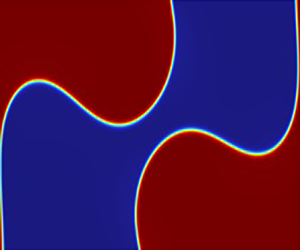
  $d_0$). The above 2-D relocation can be clearly explained by the fact that if the fluid interface and node are not perpendicular to each other, then $\boldsymbol {\nabla } \times {\boldsymbol {f}}_{rl} \neq 0$. This implies that when a sufficient energy density is applied, the fluid system in figure 4(d) will not be in equilibrium and relocation begins without imposing any perturbations unlike the other relocation discussed in this work.

Figure 4. Stabilization and relocation of inhomogeneous fluids using generalized body force  ${\boldsymbol {f}}_{ac}$ in (2.2) along with the first-order pressure field ( $|p_1|=\sqrt {real(p_1^{\star }p_1)}$) for different fluid configurations. One-dimensional (1-D) actuation is imposed on configurations shown in (a–c), and two-dimensional (2-D) actuation is imposed on configurations shown in (d). (a) HLH configuration remains stable up to $E_{ac}=85.58\ {\rm J}\ {\rm m}^{-3}$ ( $p_a = 0.67\ {\rm MPa}, d_0 = 0.21\ {\rm nm}, \nu =1.73\ {\rm MHz}$). (b) HLH configuration undergoes relocation above $E_{ac}=86.22\ {\rm J}\ {\rm m}^{-3}$ ( $p_a = 0.69\ {\rm MPa}, d_0 = 0.22\ {\rm nm}, \nu =1.73\ {\rm MHz}$). Significant variation in $|p_1|$ during relocation is observed. (c) HL configuration where the fluid interface coincides with the node remains in stable equilibrium even at $E_{ac}=2334\ {\rm J}\ {\rm m}^{-3}$ ( $p_a = 3.54\ {\rm MPa}, d_0 = 20\ {\rm nm}, \nu =1.73\ {\rm MHz}$). (d) Relocation of HL configuration due to 2-D wall actuation $(\,p_a=1.37\ {\rm MPa}, d_0=20\ {\rm nm}, \nu =2.1\ {\rm MHz})$.
3.3. Characterization of stable and unstable (relocation) regime
When the 1-D acoustic standing wave is imposed on fluids with interfacial tension, the configurations (figures 1b, 2b-i and 3a) having high impedance fluid at the anti-node and low impedance fluid at the node, become conditionally stable. From (2.21), it is evident that the stability of the above inhomogeneous fluid configurations is governed by the ratio of  $F_{rl}$ and $F_{int}$, which is called the acoustic Bond number ( $Bo_{a}$) similar to other acoustic dimensionless numbers (Mitas, Manor & Thiele Reference Mitas, Manor and Thiele2021; Muñoz et al. Reference Muñoz, Arcos, Campos-Silva, Bautista and Méndez2021):
 \begin{equation} Bo_{a}=\frac{F_{rl}}{F_{int}}=\frac{\phi E_{a c} \Delta Z \sin \left(2 k_{w} x_s\right)}{k_{h}^{2} T}. \end{equation}
The  $Bo_a$ that separates the stable and unstable region is called the critical acoustic Bond number $Bo_{a,cr}$. From (2.21),
 \begin{equation} Bo_{a,cr}=1. \end{equation}
For  $Bo_a>Bo_{a,cr}$, the above configurations become unstable (relocation occurs) and for $Bo_a< Bo_{a,cr}$, the configurations remain stable. Figure 5 shows the simulation results of different immiscible fluid combinations. The relocation and non-relocation regimes predicted by the simulations are in line with (3.2). It must also be noted that the fluids with higher interfacial tension require a higher acoustic force for relocation.
3.4. Effect of the height of the channel on stability
The height of the channel  $h$ plays a critical role in the stability of immiscible fluids. For a given $E_{ac}$, the increase in $h$ weakens the stabilizing effect of the interfacial tension force, as analysed theoretically in § 2. From (2.22), it can be inferred that the critical acoustic energy density is inversely proportional to the square of the channel height $(E_{cr} \propto 1/h^2)$. In figure 6(a), for a microchannel of height $h=80\ \mathrm {\mu } {\rm m}$ consisting of mineral–silicone oil with an interfacial tension $T=1\ {\rm mN}\ {\rm m}^{-1}$, the fluid system is stable as the applied $E_{ac}\ (120\ {\rm J}\ {\rm m}^{-3}$) is lower than the critical energy density ( $E_{cr}=384\ {\rm J}\ {\rm m}^{-3}$). However, for $h=160\ \mathrm {\mu } {\rm m}$ and keeping the remaining parameters the same, fluid relocation is observed as the applied $E_{ac}\ (120\ {\rm J}\ {\rm m}^{-3})$ is higher than the critical energy density $(E_{cr}=88.78\ {\rm J}\ {\rm m}^{-3})$.

Figure 6. Effect of channel height on stability: (a) channel height  $h= 80\ \mathrm {\mu } {\rm m}$ – no relocation is observed as applied energy density $(E_{ac} = 120\ {\rm J}\ {\rm m}^{-3})$ is less than the critical energy density $(E_{cr} = 384\ {\rm J}\ {\rm m}^{-3})$; (b) channel height $h = 160\ \mathrm {\mu } {\rm m}$ – relocation is observed as applied energy density $(E_{ac} = 120 {\rm J}\ {\rm m}^{-3})$ is high than the critical energy density $(E_{cr} = 88.78\ {\rm J}\ {\rm m}^{-3})$. This demonstrates that the interfacial tension force weakens as the height of the channel increases and thus a higher height of the channel results in a lower $E_{ac}$ required for relocation as $(E_{cr}\propto 1/h^2)$.
The above discussion on the effect of channel height on acoustic relocation has high relevance in practical applications. To relocate fluids with a high interfacial tension of  $(O(10^1 {\rm mN}\ {\rm m}^{-1}\unicode{x2013}10^2\ {\rm mN}\ {\rm m}^{-1}))$, in commonly used acoustofluidic channels of height (depth) ranging from $100\ \mathrm {\mu } {\rm m}$ to $200\ \mathrm {\mu } {\rm m}$, the required $E_{ac}$ becomes ${\approx }O(10^4)\ {\rm J}\ {\rm m}^{-3}$, which is very high compared with the $E_{ac}$ employed in typical acoustofluidic experiments $(O(10^2\ {\rm J}\ {\rm m}^{-3}\unicode{x2013}10^3 \ {\rm J}\ {\rm m}^{-3}))$. Equation (2.22) tells that the above problem can be solved by increasing the channel height as $E_{ac} \propto 1/h^2$. Hence, the height (depth) of the channel is a crucial aspect to be considered during the fabrication of an acoustofluidic microchannel for handling high interfacial tension fluids.
4. Conclusion
We have theoretically established the stability criteria for inhomogeneous fluids subjected to standing acoustic fields, which is consistent with the previous experimental investigations on miscible (Deshmukh et al. Reference Deshmukh, Brzozka, Laurell and Augustsson2014; Karlsen et al. Reference Karlsen, Augustsson and Bruus2016) and immiscible fluids (Hemachandran et al. Reference Hemachandran, Karthick, Laurell and Sen2019). Numerical simulations using a simplified and generalized acoustic body force were carried out to understand the various parameters that contribute towards the stability and relocation of fluids. However, the effect of viscous boundary layer-driven acoustic streaming on relocation is neglected in this work, which will be addressed in an upcoming paper. The insights gained from this study can have potential applications in inhomogeneous fluid handling and particle manipulation in the field of acoustofluidics.
Funding
This work was supported by the Department of Science  $\&$ Technology – Science and Engineering Research Board (DST-SERB) via grant no. SRG/2021/002180 and the Department of Science and Technology – Fund for Improvement of Science and Technology Infrastructure (DST-FIST) via grant no. SR/FST/ET-I/2021/815.
Declaration of interests
The authors report no conflict of interest.
Appendix A. First-order fields in the frequency domain
The first-order fields (fast time scale) on the frequency domain are written as
 $$\begin{gather} -{\rm i}\omega\rho_1=\boldsymbol{\nabla}\boldsymbol{\cdot}(\rho{\boldsymbol{v}}_1), \end{gather}$$
 $$\begin{gather}-{\rm i}\omega\rho{\boldsymbol{v}}_1 =-\boldsymbol{\nabla}p_1 + \eta\nabla^2 {\boldsymbol{v}}_1 + \beta\eta\boldsymbol{\nabla}(\boldsymbol{\nabla}\boldsymbol{\cdot}{\boldsymbol{v}}_1), \end{gather}$$
 $$\begin{gather}-{\rm i}\omega\rho\kappa p_1=-{\rm i}\omega\rho_1+{\boldsymbol{v}}_1\boldsymbol{\cdot} \boldsymbol{\nabla}\rho. \end{gather}$$
Also, combining (A1a) and (A1c), we get
 \begin{equation} -{\rm i}\omega\kappa p_1=-\boldsymbol{\nabla}\boldsymbol{\cdot}{\boldsymbol{v}}_1, \end{equation}
where  $p_1$ is the first-order pressure field, $\rho _1$ refers to first-order density field, ${\boldsymbol {v}}_1$ is the first-order velocity field, $\rho$ is the slow time scale density, $\kappa$ is the slow time scale compressibility, $\omega$ is the angular frequency, $\eta$ is the dynamic viscosity of the fluid, $\xi$ is the volume fluid viscosity and $\beta =(\xi /\eta )+(1/3)$. The detailed analysis of first-order and second-order fields acting on inhomogeneous fluids is given by Rajendran et al. (Reference Rajendran, Jayakumar, Azharudeen and Subramani2022).


